A Comparison between Invariant and Equivariant Classical and Quantum Graph Neural Networks

Abstract

Machine learning algorithms are heavily relied on to understand the vast amounts of data from high-energy particle collisions at the CERN Large Hadron Collider (LHC). The data from such collision events can naturally be represented with graph structures. Therefore, deep geometric methods, such as graph neural networks (GNNs), have been leveraged for various data analysis tasks in high-energy physics. One typical task is jet tagging, where jets are viewed as point clouds with distinct features and edge connections between their constituent particles. The increasing size and complexity of the LHC particle datasets, as well as the computational models used for their analysis, have greatly motivated the development of alternative fast and efficient computational paradigms such as quantum computation. In addition, to enhance the validity and robustness of deep networks, we can leverage the fundamental symmetries present in the data through the use of invariant inputs and equivariant layers. In this paper, we provide a fair and comprehensive comparison of classical graph neural networks (GNNs) and equivariant graph neural networks (EGNNs) and their quantum counterparts: quantum graph neural networks (QGNNs) and equivariant quantum graph neural networks (EQGNN). The four architectures were benchmarked on a binary classification task to classify the parton-level particle initiating the jet. Based on their area under the curve (AUC) scores, the quantum networks were found to outperform the classical networks. However, seeing the computational advantage of quantum networks in practice may have to wait for the further development of quantum technology and its associated application programming interfaces (APIs).

1. Introduction

Through the measurement of the byproducts of particle collisions, the Large Hadron Collider (LHC) collects a substantial amount of information about fundamental particles and their interactions. The data produced from these collisions can be analyzed using various supervised and unsupervised machine learning methods [1,2,3,4,5]. Jet tagging is a key task in high-energy physics, which seeks to identify the likely parton-level particle from which the jet originated. By viewing individual jets as point clouds with distinct features and edge connections between their constituent particles, a graph neural network (GNN) is considered a well-suited architecture for jet tagging [2,3].

Classified as deep geometric networks, GNNs have the potential to draw inferences about a graph structure, including the interactions among the elements in the graph [6,7]. Graph neural networks are typically thought of as generalizations of convolutional neural networks (CNNs), which are predominantly used for image recognition, pattern recognition, and computer vision [8,9]. This can be attributed to the fact that in an image, each pixel is connected to its nearest neighboring pixels, whereas in a general dataset, one would ideally like to construct an arbitrary graph structure among the samples. Many instances in nature can be described well in terms of graphs, including molecules, maps, social networks, and the brain. For example, in molecules, the nodal data can be attributed to the atoms, the edges can be characterized as the strength of the bond between atoms, and the features embedded within each node can be the atom’s characteristics, such as reactivity.

Generally, graphically structured problems involve unordered sets of elements with a learnable embedding of the input features. Useful information can be extracted from such graphically structured data by embedding them within GNNs. Many subsequent developments have been made to GNNs since their first implementation in 2005. These developments have included graph convolutional, recurrent, message passing, graph attention, and graph transformer architectures [2,6,10,11].

To enhance the validity and robustness of deep networks, invariant and equivariant networks have been constructed to learn the symmetries embedded within a dataset by preserving an oracle in the former and by enforcing weight sharing across filter orientations in the latter [12,13]. Utilizing analytical invariant quantities characteristic of physical symmetry representations, computational methods have successfully rediscovered fundamental Lie group structures, such as the $SO\left(n\right)$, $SO(1,3)$, and $U\left(n\right)$ groups [14,15,16,17]. Nonlinear symmetry discovery methods have also been applied to classification tasks in data domains [18]. The simplest and most useful embedded symmetry transformations include translations, rotations, and reflections, which have been the primary focus in invariant (IGNN) and equivariant (EGNN) graph neural networks [19,20,21].

The learned representations from the collection of these network components can be used to understand unobservable causal factors, uncover fundamental physical principles governing these processes, and possibly even discover statistically significant hidden anomalies. However, with increasing amounts of available data and the computational cost of these deep learning networks, large computing resources will be required to efficiently run these machine learning algorithms. The extension of classical networks, which rely on bit-wise computation, to quantum networks, which rely on qubit-wise computation, is already underway as a solution to this complexity problem. Due to superposition and entanglement among qubits, quantum networks are able to store the equivalent of $2^n$ characteristics from n two-dimensional complex vectors. In other words, while the expressivity of the classical network scales linearly, that of the quantum network scales exponentially with the sample size n [22]. Many APIs, including Xanadu’s Pennylane, Google’s Cirq, and IBM’s Qiskit, have been developed to allow for the testing of the quantum circuits and quantum machine learning algorithms running on these quantum devices.

In the quantum graph structure, classical nodes can be mapped to the quantum states of the qubits, real-valued features to the complex-valued entries of the states, edges to the interactions between states, and edge attributes to the strength of the interactions between the quantum states. Through a well-defined Hamiltonian operator, the larger structure of a classical model can then be embedded into the quantum model. The unitary operator constructed from this parameterized Hamiltonian determines the temporal evolution of the quantum system by acting on the fully entangled quantum state of the graph. Following several layers of application, a final state measurement of the quantum system can then be made to reach a final prediction. The theory and application of unsupervised and supervised learning tasks involving quantum graph neural networks (QGNNs), quantum graph recurrent neural networks (QGRNNs), and quantum graph convolutional neural networks (QGCNNs) have already been developed [23,24]. Improvements to these models to arbitrarily sized graphs have been made with the implementation of ego-graph-based quantum graph neural networks (egoQGNNs) [25]. Quantum analogs of other advanced classical architectures, including generative adversarial networks (GANs), transformers, natural language processors (NLPs), and equivariant networks, have also been proposed [23,26,27,28,29,30,31,32].

With the rapid development of quantum deep learning, this paper intends to offer a fair and comprehensive comparison between classical GNNs and their quantum counterparts. To classify whether a particle jet has originated from a quark or a gluon, a binary classification task was carried out using four different architectures. These architectures included a GNN, SE(2) EGNN, QGNN, and permutation EQGNN. Each quantum model was fine tuned to have an analogous structure to its classical form. In order to provide a fair comparison, all models used similar hyperparameters as well as a similar number of total trainable parameters. The final results across each architecture were recorded using identical training, validation, and testing sets. We found that QGNN and EQGNN outperformed their classical analogs on the particular binary classification task described above. Although these results seem promising for the future of quantum computing, the further development of quantum APIs is required to allow for more general implementations of quantum architectures.

2. Data

The jet tagging binary classification task is illustrated with the high-energy physics (HEP) dataset Pythia8 Quark and Gluon Jets for Energy Flow [33]. This dataset contains data from two million particle collision jets split equally into one million jets that originated from a quark and one million jets that originated from a gluon. These jets resulted from LHC collisions with total center of mass energy $\sqrt{s}=14$ TeV and were selected to have transverse momenta $p_T^{jet}$ between 500 to 550 GeV and rapidities $|y^{jet}|<1.7$. The jet kinematic distributions are shown in Figure 1. For each jet $\alpha$, the classification label is provided as either a quark with $y_{\alpha }=1$ or a gluon with $y_{\alpha }=0$. Each particle i within the jet is listed with its transverse momentum $p_{T,\alpha }^{\left(i\right)}$, rapidity $y_{\alpha }^{\left(i\right)}$, azimuthal angle ${\varphi }_{\alpha }^{\left(i\right)}$, and PDG id $I_{\alpha }^{\left(i\right)}$.

Figure 1. Distributions of the jet transverse momenta $p_T$, total momenta p, and energies E.

2.1. Graphically Structured Data

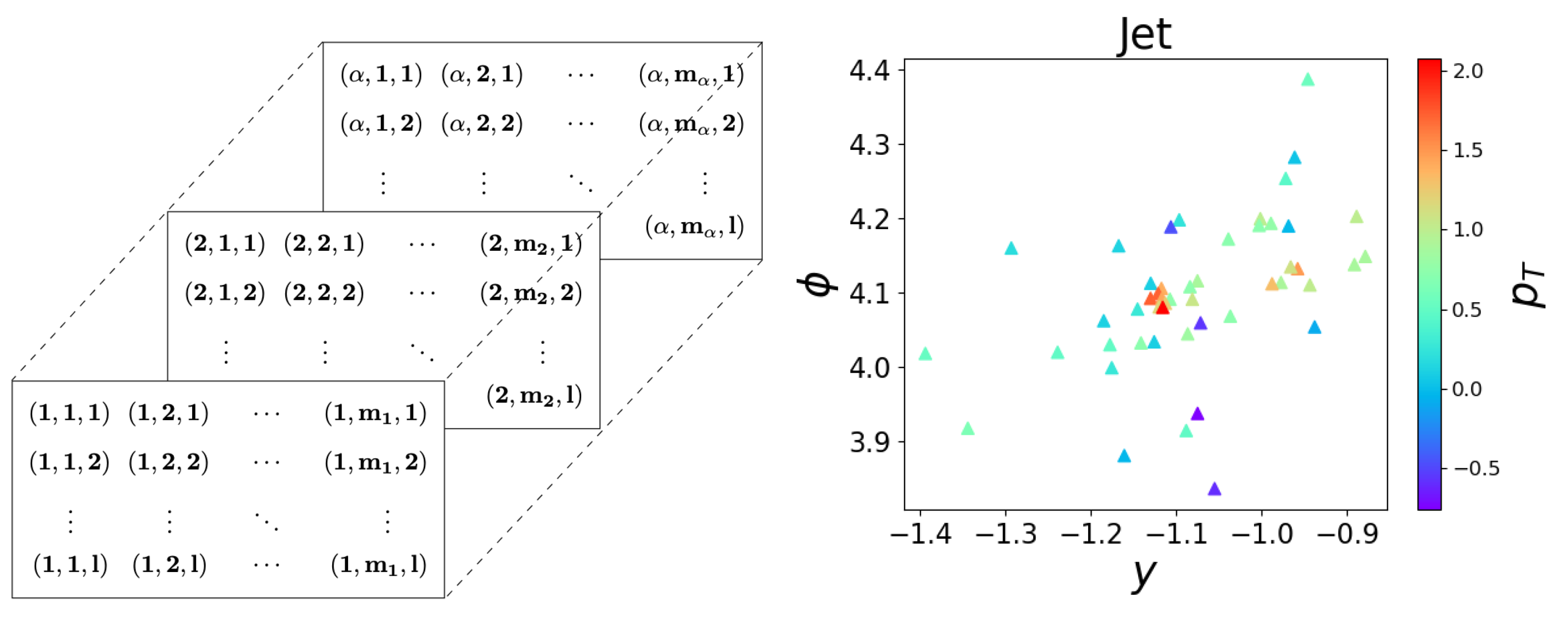
A graph $\mathcal{G}$ is typically defined as a set of nodes $\mathcal{V}$ and edges $\mathcal{E}$, i.e., $\mathcal{G}=\{\mathcal{V},\mathcal{E}\}$. Each node $v^{\left(i\right)}\in \mathcal{V}$ is connected to its neighboring nodes $v^{\left(j\right)}$ via edges $e^{\left(ij\right)}\in \mathcal{E}$. In our case, each jet $\alpha$ can be considered as a graph ${\mathcal{J}}_{\alpha }$ composed of the jet’s constituent particles as the nodes $v_{\alpha }^{\left(i\right)}$ with node features $h_{\alpha }^{\left(il\right)}$ and edge connections $e_{\alpha }^{\left(ij\right)}$ between the nodes in ${\mathcal{J}}_{\alpha }$ with edge features $a_{\alpha }^{\left(ij\right)}$. It should be noted that the number of nodes within a graph can vary. This is especially true for the case of particle jets, where the number of particles within each jet can vary greatly. Each jet ${\mathcal{J}}_{\alpha }$ can be considered as a collection of $m_{\alpha }$ particles with l distinct features per particle. An illustration of graphically structured data and an example jet in the $(\varphi ,y)$ plane are shown in Figure 2.

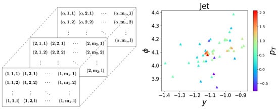
Figure 2. A visualization of graphically structured data (left) and a sample jet shown in the $(\varphi ,y)$ plane (right) with each particle color-coded by its transverse momentum $p_{T,\alpha }^{\left(i\right)}$.

2.2. Feature Engineering

We used the Particle package [34] to find the particle masses $m_{\alpha }^{\left(i\right)}$ from the respective particle IDs $I_{\alpha }^{\left(i\right)}$. From the available kinematic information for each particle i, we constructed new physically meaningful kinematic variables [35], which were used as additional features in the analysis. In particular, we considered the transverse mass $m_{T,\alpha }^{\left(i\right)}$, the energy $E_{\alpha }^{\left(i\right)}$, and the Cartesian momentum components, $p_{x,\alpha }^{\left(i\right)}$, $p_{y,\alpha }^{\left(i\right)}$, and $p_{z,\alpha }^{\left(i\right)}$, defined, respectively, as

$$\begin{array}{cc}\hfill m_{T,\alpha }^{\left(i\right)}& =\sqrt{m_{\alpha }^{\left(i\right)2}+p_{T,\alpha }^{\left(i\right)2}},E_{\alpha }^{\left(i\right)}=m_{T,\alpha }^{\left(i\right)}\cos \mathrm{h}\left(y_{\alpha }^{\left(i\right)}\right),\hfill \\ \hfill p_{x,\alpha }^{\left(i\right)}& =p_{T,\alpha }^{\left(i\right)}\cos \left({\varphi }_{\alpha }^{\left(i\right)}\right),p_{y,\alpha }^{\left(i\right)}=p_{T,\alpha }^{\left(i\right)}\sin \left({\varphi }_{\alpha }^{\left(i\right)}\right),p_{z,\alpha }^{\left(i\right)}=m_{T,ij}\sin \mathrm{h}\left(y_{\alpha }^{\left(i\right)}\right).\hfill \end{array}$$

(1)

The original kinematic information in the dataset was then combined with the additional kinematic variables (1) into a feature set $h_{\alpha }^{\left(il\right)}$, $l=0,1,2,\dots ,7$, as follows:

$$h_{\alpha }^{\left(il\right)}\equiv \left\{p_{T,\alpha }^{\left(i\right)},y_{\alpha }^{\left(i\right)},{\varphi }_{\alpha }^{\left(i\right)},m_{T,\alpha }^{\left(i\right)},E_{\alpha }^{\left(i\right)},p_{x,\alpha }^{\left(i\right)},p_{y,\alpha }^{\left(i\right)},p_{z,\alpha }^{\left(i\right)}\right\}.$$

(2)

These features were then max-scaled by their maximum value across all jets $\alpha$ and particles i, i.e., $h_{\alpha }^{\left(il\right)}\to h_{\alpha }^{\left(il\right)}/ma{x}_{\alpha ,i}\left(h_{\alpha }^{\left(il\right)}\right)$.

Edge connections are formed via the Euclidean distance $\Delta R=\sqrt{\Delta {\varphi }^2+\Delta y^2}$ between one particle and its neighbor in $(\varphi ,y)$ space. Therefore, the edge attribute matrix for each jet can be expressed as

$$\begin{array}{c}\hfill a_{\alpha }^{\left(ij\right)}\equiv \Delta R_{\alpha }^{\left(ij\right)}=\sqrt{{\left({\varphi }_{\alpha }^{\left(i\right)}-{\varphi }_{\alpha }^{\left(j\right)}\right)}^2+{\left(y_{\alpha }^{\left(i\right)}-y_{\alpha }^{\left(j\right)}\right)}^2}.\end{array}$$

(3)

2.3. Training, Validation, and Testing Sets

We considered jets with at least 10 particles. This left us with N = 1,997,445 jets, 997,805 of which were quark jets. While the classical GNN is more flexible in terms of its hidden features, the size of the quantum state and the Hamiltonian scale as $2^n$, where n is the number of qubits. As we shall see, the number of qubits is given by the number of nodes $n_{\alpha }$ in the graph, i.e., the number of particles in the jet. Therefore, jets with large particle multiplicity require prohibitively complex quantum networks. Thus, we limited ourselves to the case of $n_{\alpha }=3$ particles per jet by only considering the three highest momenta $p_T$ particles within each jet. In other words, each graph contained the set ${\mathbf{h}}_{\alpha }=({\mathbf{h}}_{\alpha }^{\left(1\right)},{\mathbf{h}}_{\alpha }^{\left(2\right)},{\mathbf{h}}_{\alpha }^{\left(3\right)})$, where each ${\mathbf{h}}_{\alpha }^{\left(i\right)}\in {\mathbb{R}}^8$ and ${\mathbf{h}}_{\alpha }\in {\mathbb{R}}^{3\times 8}$. For training, we randomly picked N = 12,500 jets and used the first 10,000 for training, the next 1250 for validation, and the last 1250 for testing. These sets happened to contain 4982, 658, and 583 quark jets, respectively.

3. Models

The four different models described below, including a GNN, an EGNN, a QGNN, and an EQGNN, were constructed to perform graph classification. The binary classification task was determining whether a jet ${\mathcal{J}}_{\alpha }$ originated from a quark or a gluon.

3.1. Invariance and Equivariance

By making a network invariant or equivariant to particular symmetries within a dataset, a more robust architecture can be developed. In order to introduce invariance and equivariance, one must assume or learn a certain symmetry group G of transformations on the dataset. A function $\phi :X\to Y$ is equivariant with respect to a set of group transformations $T_g:X\to X$, $g\in G$, acting on the input vector space X, if there exists a set of transformations $S_g:Y\to Y$ that similarly transform the output space Y, i.e.,

$$\begin{array}{c}\hfill \phi \left(T_{g}x\right)=S_g\phi \left(x\right).\end{array}$$

(4)

A model is said to be invariant when, for all $g\in G$, $S_g$ becomes the set containing only the trivial mapping, i.e., $S_g=\left\{{\mathbb{I}}_G\right\}$, where ${\mathbb{I}}_G\in G$ is the identity element of the group G [12,36].

Invariance performs better as an input embedding, whereas equivariance can be more easily incorporated into the model layers. For each model, the invariant component corresponds to the translational and rotational invariant embedding distance $\phi \equiv \Delta R_{\alpha }^{\left(ij\right)}$. Here, the function $\phi :{\mathbb{R}}^2\times {\mathbb{R}}^2\to \mathbb{R}$ makes up the edge attribute matrix $a_{\alpha }^{\left(ij\right)}$, as defined in Equation (3). This distance is used as opposed to solely incorporating the raw coordinates. Equivariance has been accomplished through the use of simple nontrivial functions along with higher-order methods involving the use of spherical harmonics to embed the equivariance within the network [37,38]. Equivariance takes different forms in each model presented here.

3.2. Graph Neural Network

Classical GNNs take in a collection of graphs $\left\{{\mathcal{G}}_{\alpha }\right\}$, each with nodes $v_{\alpha }^{\left(i\right)}\in {\mathcal{V}}_{\alpha }$ and edges $e_{\alpha }^{\left(ij\right)}\in {\mathcal{E}}_{\alpha }$, where each graph ${\mathcal{G}}_{\alpha }=\{{\mathcal{V}}_{\alpha },{\mathcal{E}}_{\alpha }\}$ is the set of its corresponding nodes and edges. Each node $v_{\alpha }^{\left(i\right)}$ has an associated feature vector $h_{\alpha }^{\left(il\right)}$, and the entire graph has an associated edge attribute tensor $a_{\alpha }^{\left(ijr\right)}$ describing r different relationships between node $v_{\alpha }^{\left(i\right)}$ and its neighbors $v_{\alpha }^{\left(j\right)}$. Here, we can define $\mathcal{N}\left(i\right)$ as the set of neighbors of node $v_{\alpha }^{\left(i\right)}$ and take $r=1$, as we only consider one edge attribute. In other words, the edge attribute tensor $a_{\alpha }^{\left(ijr\right)}\to a_{\alpha }^{\left(ij\right)}$ becomes a matrix. The edge attributes are typically formed from the features corresponding to each node and its neighbors.

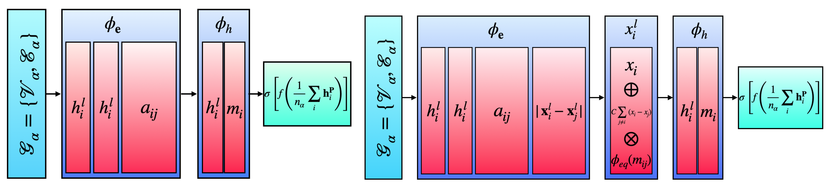
In the layer structure of a GNN, multilayer perceptions (MLPs) are used to update the node features and edge attributes before aggregating, or mean pooling, the updated node features for each graph to make a final prediction. To simplify notation, we omit the graph index $\alpha$, lower the node index i, and introduce a model layer index l. The first MLP is the edge MLP ${\varphi }_e$, which, at each layer l, collects the features ${\mathbf{h}}_i^l$, its neighbors’ features ${\mathbf{h}}_j^l$, and the edge attribute $a_{ij}$ corresponding to the pair. Once the new edge matrix $m_{ij}$ is formed, we sum along the neighbor dimension j to create a new node feature ${\mathbf{m}}_i$. This extra feature is then added to the original node features ${\mathbf{h}}_i$ before being input into a second node updating MLP ${\varphi }_h$ to form new node features $h_i^{l+1}$ [8,10,21]. Therefore, a GNN is defined as

$$\begin{array}{cc}\hfill {\mathbf{m}}_{ij}& ={\varphi }_e({\mathbf{h}}_i^l,{\mathbf{h}}_j^l,a_{ij}),\hfill \\ \hfill {\mathbf{m}}_i& ={\displaystyle \sum _{j\in \mathcal{N}\left(i\right)}}{\mathbf{m}}_{ij},\hfill \\ \hfill {\mathbf{h}}_i^{l+1}& ={\varphi }_h({\mathbf{h}}_i^l,{\mathbf{m}}_i).\hfill \end{array}$$

(5)

Here, $h_i^l\in {\mathbb{R}}^k$ is the kth-dimensional embedding of node $v_i$ at layer l, and ${\mathbf{m}}_{ij}$ is typically referred to as the message-passing function. Once the data are sent through the P graph layers of the GNN, the updated nodes ${\mathbf{h}}_i^P$ are aggregated via mean pooling for each graph to form a set of final features $\frac{1}{n_{\alpha }}{\displaystyle {\sum }_{i=1}^{n_{\alpha }}}{\mathbf{h}}_i^P$. These final features are sent through a fully connected neural network (NN) to output the predictions. Typically, a fixed number of hidden features $k=N_h$ is defined for both the edge and node MLPs. The described GNN architecture is pictorially shown in the left panel in Figure 3.

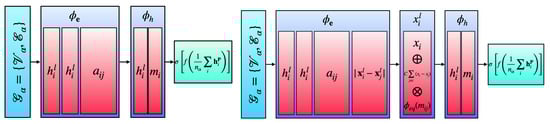
Figure 3. Graph neural network (GNN, left) and equivariant graph neural network (EGNN, right) schematic diagrams.

3.3. SE(2) Equivariant Graph Neural Network

For the classical EGNN, the approach used here was informed by the successful implementation of SE(3), or rotational, translational, and permutational, equivariance on dynamic systems and the QM9 molecular dataset [21]. It should be noted that GNNs are naturally permutation equivariant, in particular invariant, when averaging over the final node feature outputs of the graph layers [39]. An SE(2) EGNN takes the same form as a GNN; however, the coordinates are equivariantly updated within each graph layer, i.e., ${\mathbf{x}}_i\to {\mathbf{x}}_i^l$ where ${\mathbf{x}}_i=({\varphi }_i,y_i)$ in our case. The new form of the network becomes

$$\begin{array}{cc}\hfill {\mathbf{m}}_{ij}& ={\varphi }_e({\mathbf{h}}_i^l,{\mathbf{h}}_j^l,a_{ij},|{\mathbf{x}}_i^l-{\mathbf{x}}_j^l\left|\right),\hfill \\ \hfill {\mathbf{m}}_i& ={\displaystyle \sum _{j\in \mathcal{N}\left(i\right)}}{\mathbf{m}}_{ij},\hfill \\ \hfill {\mathbf{x}}_i^{l+1}& ={\mathbf{x}}_i^l+C{\displaystyle \sum _{j\ne i}}({\mathbf{x}}_i^l-{\mathbf{x}}_j^l){\varphi }_x\left({\mathbf{m}}_{ij}\right),\hfill \\ \hfill {\mathbf{h}}_i^{l+1}& ={\varphi }_h({\mathbf{h}}_i^l,{\mathbf{m}}_i).\hfill \end{array}$$

(6)

Since the coordinates ${\mathbf{x}}_i^l$ of each node $v_i$ are equivariantly evolving, we also introduce a second invariant embedding $|{\mathbf{x}}_i^l-{\mathbf{x}}_j^l|$ based on the equivariant coordinates into the edge MLP ${\varphi }_e$. The coordinates ${\mathbf{x}}_i$ are updated by adding the summed difference between the coordinates of ${\mathbf{x}}_i$ and its neighbors ${\mathbf{x}}_j$. This added term is suppressed by a factor of C, which we take to be $C\left(n_{\alpha }\right)=\frac{1}{ln\left(2n_{\alpha }\right)}$. The term is further multiplied by a coordinate MLP ${\varphi }_x,$ which takes as input the message-passing function ${\mathbf{m}}_{ij}$ between node i and its neighbors j. For a proof of the rotational and translational equivariance of ${\mathbf{x}}_i^{l+1}$, see Appendix A. The described EGNN architecture is pictorially shown in the right panel in Figure 3.

3.4. Quantum Graph Neural Network

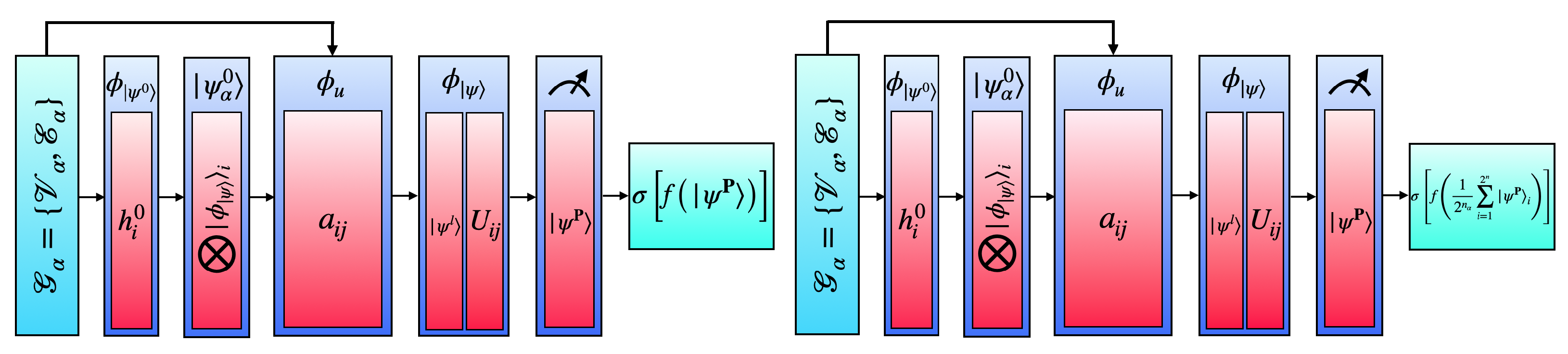
For a QGNN, the input data, as a collection of graphs $\left\{{\mathcal{G}}_{\alpha }\right\}$, are the same as described above. We fix the number of qubits n to be the number of nodes $n_{\alpha }$ in each graph. For the quantum algorithm, we first form a normalized qubit product state from an embedding MLP ${\varphi }_{|{\psi }^0⟩}$, which takes in the features ${\mathbf{h}}_i$ of each node $v_i$ and reduces each of them to a qubit state $|{\varphi }_{|{\psi }^0⟩}\left({\mathbf{h}}_i\right)⟩\in {\mathbb{C}}^2$ [40]. The initial product state describing the system then becomes $|{\psi }_{\alpha }^0⟩={\displaystyle {⨂}_{i=1}^n}|{\varphi }_{|\psi ⟩}\left({\mathbf{h}}_i\right)⟩\in {\mathbb{C}}^{2^n}$, which we normalize by $\sqrt{⟨{\psi }_{\alpha }^0|{\psi }_{\alpha }^0⟩}$.

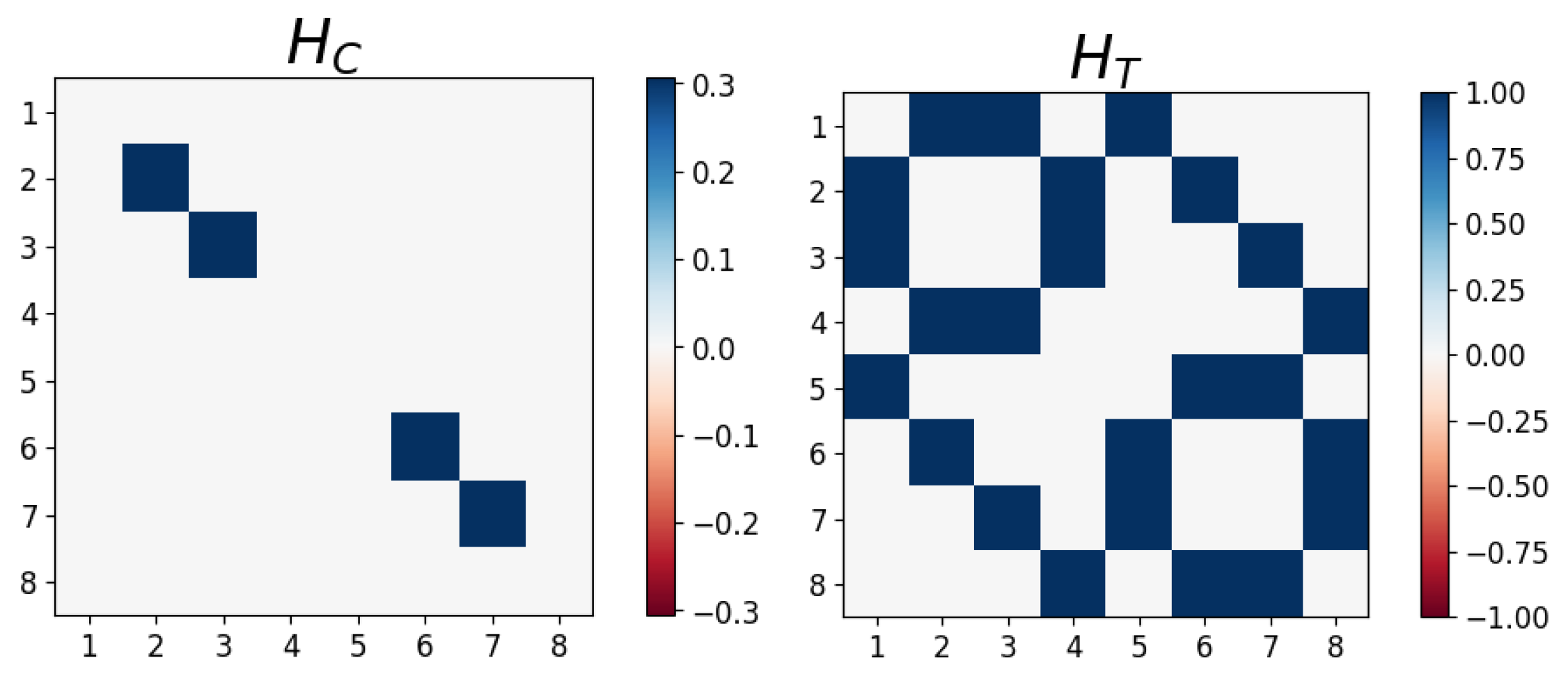
A fully parameterized Hamiltonian can then be constructed based on the adjacency matrix $a_{ij}$, or trainable interaction weights ${\mathcal{W}}_{ij}$, and node features ${\mathbf{h}}_i$, or trainable feature weights ${\mathcal{M}}_i$ [24]. Here, for the coupling term of the Hamiltonian $H_C$, we utilize the edge matrix $a_{ij}$ connected to two coupled Pauli-Z operators, ${\sigma }_i^z$ and ${\sigma }_j^z$, which act on the Hilbert spaces of qubits i and j, respectively. Since we embed the quantum state $|{\psi }^0⟩$ based on the node features ${\mathbf{h}}_i$, we omit the self-interaction term which utilizes the chosen features applied to the Pauli-Z operator, ${\sigma }_i^z$, which acts on the Hilbert space of qubit i. We also introduce a transverse term $H_T$ to each node in the form of a Pauli-X operator, ${\sigma }_i^x$, with a fixed or learnable constant coefficient ${\mathcal{Q}}_0$, which we take to be ${\mathcal{Q}}_0=1$. Note that the Hamiltonian H contains $\mathcal{O}(2^n\times 2^n)$ entries due to the Kronecker products between Pauli operators. To best express the properties of each graph, we take the Hamiltonian of the form

$$\begin{array}{cc}\hfill H\left(a_{ij}\right)& =\underset{H_C}{\underbrace{{\displaystyle {\sum }_{(i,j)\in \mathcal{E}}}{a}_{ij}{\left(\frac{{\widehat{\mathbb{I}}}_i-{\sigma }_i^z}{2}-\frac{{\widehat{\mathbb{I}}}_j-{\sigma }_j^z}{2}\right)}^2}}+\underset{H_T}{\underbrace{{\displaystyle {\sum }_{i\in \mathcal{V}}}{\sigma }_i^x}},\hfill \end{array}$$

(7)

where the $8\times 8$ matrix representations of $H_C$ and $H_T$ are shown in Figure 4. We generate the unitary form of the operator via the complex exponentiating of the Hamiltonian with real learnable coefficients ${\gamma }_{lq}\in {\mathbb{R}}^{P\times Q}$, which can be thought of as infinitesimal parameters running over $Q=2$ Hamiltonian terms and P layers of the network. Therefore, the QGNN can be defined as

$$\begin{array}{cc}\hfill U_{ij}& ={\varphi }_u\left(a_{ij}\right)=e^{-i{\displaystyle {\sum }_{q=1}^Q}{\gamma }_{lq}{H}_q\left(a_{ij}\right)},\hfill \end{array}$$

(8a)

$$\begin{array}{cc}\hfill |{\psi }^{l+1}⟩& ={\varphi }_{|\psi ⟩}\left(\right|{\psi }^l⟩,U_{ij})=U_{\theta }^l{U}_{ij}{U}_{\theta }^{l^{†}}|{\psi }^l⟩,\hfill \end{array}$$

(8b)

where $U_{\theta }^l=({\mathit{\theta }}^{\prime }-i\mathbb{I}){({\mathit{\theta }}^{\prime }+i\mathbb{I})}^{-1}$ is a parameterized unitary Cayley transformation in which we force ${\mathit{\theta }}^{\prime }=\mathit{\theta }+{\mathit{\theta }}^{†}$ to be self-adjoint, i.e., ${\mathit{\theta }}^{\prime }={\mathit{\theta }}^{\prime †}$, with $\mathit{\theta }\in {\mathbb{C}}^{2^n\times 2^n}$ as the trainable parameters. The QGNN evolves the quantum state $|{\psi }^0⟩$ by applying unitarily transformed ansatz Hamiltonians with Q terms to the state over P layers.

Figure 4. The $8\times 8$ matrix representations of the coupling and transverse Hamiltonians defined in Equation (7).

The final product state $|{\psi }^P⟩ \in {\mathbb{C}}^{2^n}$ is measured for output, which is sent to a classical fully connected NN to make a prediction. The analogy between the quantum unitary interaction function ${\varphi }_u$ and classical edge MLP ${\varphi }_e$, as well as between the quantum unitary state update function ${\varphi }_{|\psi ⟩}$ and classical node update function ${\varphi }_h$, should be clear. For a reduction in the coupling Hamiltonian $H_C$ in Equation (7), see Appendix B. The described QGNN architecture is pictorially shown in the left panel in Figure 5.

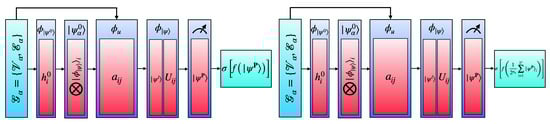
Figure 5. Quantum graph neural network (QGNN, left) and equivariant quantum graph neural network (EQGNN, right) schematic diagrams.

3.5. Permutation Equivariant Quantum Graph Neural Network

The EQGNN takes the same form as the QGNN; however, we aggregate the final elements of the product state $\frac{1}{2^n}{\displaystyle {\sum }_{k=1}^{2^n}}|{\psi }_k^P⟩$ via mean pooling before sending this complex value to a fully connected NN [31,40,41]. See Appendix C for a proof of the quantum product state permutation equivariance over the sum of its elements. The resulting EQGNN architecture is shown in the right panel in Figure 5.

4. Results and Analysis

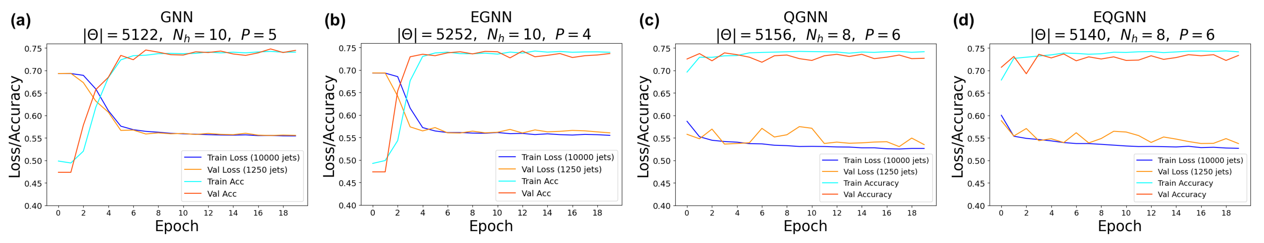
For each model, a range of total parameters was tested; however, the overall comparison test was conducted using the largest optimal number of total parameters for each network. A feed-forward NN was used to reduce each network’s graph layered output to a binary one, followed by the softmax activation function to obtain the logits in the classical case and the norm of the complex values to obtain the logits in the quantum case. Each model trained over 20 epochs with the Adam optimizer consisting of a learning rate of $\eta ={10}^{-3}$ and a cross-entropy loss function. The classical networks were trained with a batch size of 64 and the quantum networks with a batch size of one due to the limited capabilities of broadcasting unitary operators in the quantum APIs. After epoch 15, the best model weights were saved when the validation AUC of the true positive rate (TPR) as a function of the false positive rate (FPR) was maximized. The results of the training for the largest optimal total number of parameters $\left|\mathsf{\Theta }\right|\approx 5100$ are shown in Figure 6, with more details listed in Table 1.

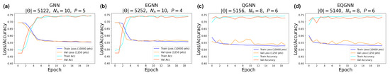
Figure 6. (a) GNN, (b) EGNN, (c) QGNN, and (d) EQGNN training history plots.

Table 1. Metric comparison between the classical and quantum graph models ¹.

Model	$\left|\mathbf{\Theta }\right|$	${\mathit{N}}_{\mathit{h}}$	P	Train ACC	Val ACC	Test AUC
GNN	5122	10	5	74.25%	74.80%	63.36%
EGNN	5252	10	4	73.66%	74.08%	67.88%
QGNN	5156	8	6	$74.00\%$	$73.28\%$	61.43%
EQGNN	5140	8	6	$74.42\%$	$72.56\%$	75.17%

¹ The pink color represents the GNN results. The red color represents the EGNN results. The blue color represents the QGNN results. The cyan color represents the EQGNN results. This representation extends to Figure 7.

Recall that for each model, we varied the number of hidden features $N_h$ in the P graph layers. Since we fixed the number of nodes $n_{\alpha }=3$ per jet, the hidden feature number $N_h=2^3=8$ was fixed in the quantum case, and, therefore, we also varied the parameters of the encoder ${\varphi }_{|{\psi }^0⟩}$ and decoder NN in the quantum algorithms.

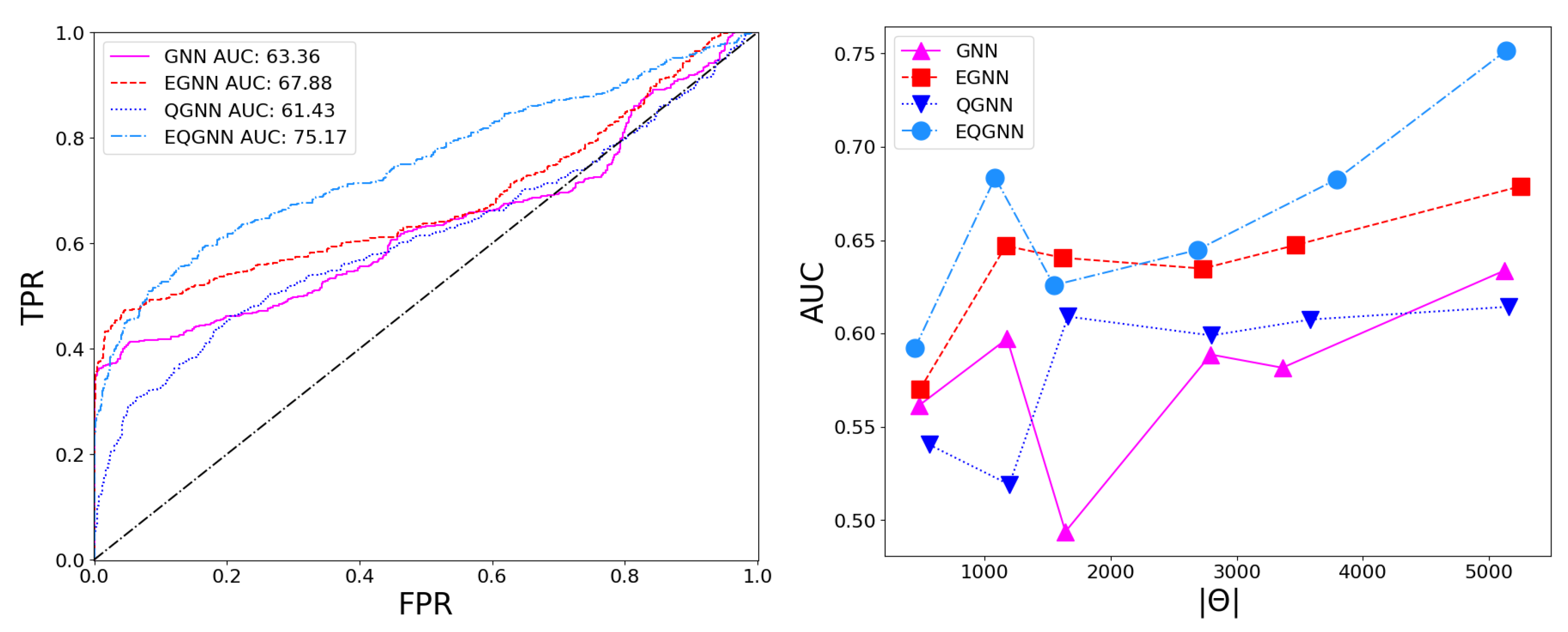
Based on the AUC scores, the EGNN outperformed both the classical and quantum GNN; however, this algorithm was outperformed by EQGNN with a $7.29\%$ increase in AUC, representing the strength of the EQGNN. Although the GNN outperformed the QGNN in the final parameter test by $1.93\%$, the QGNN performed more consistently and outperformed the GNN in the mid-parameter range $\left|\mathsf{\Theta }\right|\in (1500,4000)$. Through the variation in the number of parameters, the AUC scores were recorded for each case, where the number of parameters taken for each point corresponded to $\left|\mathsf{\Theta }\right|\approx \{500,1200,1600,2800,3500,5100\}$, as shown in the right panel in Figure 7.

Figure 7. Model ROC curves (left) and AUC scores as a function of parameters (right).

5. Conclusions

Through several computational experiments, the quantum GNNs seemed to exhibit enhanced classifier performance compared with their classical GNN counterparts based on the best test AUC scores produced after the training of the models while relying on a similar number of parameters, hyperparameters, and model structures. These results seem promising for the quantum advantage over classical models. Despite this result, the quantum algorithms took over 100 times longer to train than the classical networks. This was primarily due to the fact that we ran our quantum simulations on classical computers and not on actual quantum hardware. In addition, we were hindered by the limited capabilities in the quantum APIs, where the inability to train with broadcastable unitary operators forced the quantum models to take in a batch size of one or train on a single graph at a time.

The action of the equivariance in the EGNN and EQGNN could be further explored and developed. This is especially true in the quantum case where more general permutation and SU(2) equivariance have been explored [40,41,42,43]. Expanding the flexibility of the networks to an arbitrary number of nodes per graph should also offer increased robustness; however, this may continue to pose challenges in the quantum case due to the current limited flexibility of quantum software. A variety of different forms of the networks can also be explored. Potential ideas for this include introducing attention components and altering the structure of the quantum graph layers to achieve enhanced performance of both classical and quantum GNNs. In particular, one can further parameterize the quantum graph layer structure to better align with the total number of parameters used in the classical structures. These avenues will be explored in future work.

6. Software and Code

PyTorch and Pennylane were the primary APIs used in the formation and testing of these algorithms. The code corresponding to this study can be found at https://github.com/royforestano/2023_gsoc_ml4sci_qmlhep_gnn (accessed on 5 February 2024).

References

- Andreassen, A.; Feige, I.; Frye, C.; Schwartz, M.D. JUNIPR: A framework for unsupervised machine learning in particle physics. Eur. Phys. J. C 2019, 79, 102. [Google Scholar] [CrossRef]
- Shlomi, J.; Battaglia, P.; Vlimant, J.R. Graph neural networks in particle physics. Mach. Learn. Sci. Technol. 2020, 2, 021001. [Google Scholar] [CrossRef]
- Mikuni, V.; Canelli, F. Point cloud transformers applied to collider physics. Mach. Learn. Sci. Technol. 2021, 2, 035027. [Google Scholar] [CrossRef]
- Mokhtar, F.; Kansal, R.; Duarte, J. Do graph neural networks learn traditional jet substructure? arXiv 2022, arXiv:2211.09912. [Google Scholar]
- Mikuni, V.; Canelli, F. ABCNet: An attention-based method for particle tagging. Eur. Phys. J. Plus 2020, 135, 463. [Google Scholar] [CrossRef] [PubMed]
- Veličković, P. Everything is connected: Graph neural networks. Curr. Opin. Struct. Biol. 2023, 79, 102538. [Google Scholar] [CrossRef] [PubMed]
- Zhou, J.; Cui, G.; Hu, S.; Zhang, Z.; Yang, C.; Liu, Z.; Wang, L.; Li, C.; Sun, M. Graph neural networks: A review of methods and applications. AI Open 2020, 1, 57–81. [Google Scholar] [CrossRef]
- Kipf, T.N.; Welling, M. Semi-Supervised Classification with Graph Convolutional Networks. arXiv 2016, arXiv:1609.02907. [Google Scholar]
- Kipf, T.N.; Welling, M. Semi-Supervised Classification with Graph Convolutional Networks. In Proceedings of the 5th International Conference on Learning Representations (ICLR ’17), Toulon, France, 24–26 April 2017. [Google Scholar]
- Gilmer, J.; Schoenholz, S.S.; Riley, P.F.; Vinyals, O.; Dahl, G.E. Neural Message Passing for Quantum Chemistry. In Proceedings of the 34th International Conference on Machine Learning, Sydney, Australia, 6–11 August 2017; Volume 70, pp. 1263–1272. [Google Scholar]
- Veličković, P.; Cucurull, G.; Casanova, A.; Romero, A.; Liò, P.; Bengio, Y. Graph Attention Networks. In Proceedings of the International Conference on Learning Representations, Vancouver, BC, Canada, 30 April–3 May 2018. [Google Scholar]
- Lim, L.; Nelson, B.J. What is an equivariant neural network? arXiv 2022, arXiv:2205.07362. [Google Scholar] [CrossRef]
- Ecker, A.S.; Sinz, F.H.; Froudarakis, E.; Fahey, P.G.; Cadena, S.A.; Walker, E.Y.; Cobos, E.; Reimer, J.; Tolias, A.S.; Bethge, M. A rotation-equivariant convolutional neural network model of primary visual cortex. In Proceedings of the International Conference on Learning Representations, New Orleans, LA, USA, 6–9 May 2019. [Google Scholar]
- Forestano, R.T.; Matchev, K.T.; Matcheva, K.; Roman, A.; Unlu, E.B.; Verner, S. Deep learning symmetries and their Lie groups, algebras, and subalgebras from first principles. Mach. Learn. Sci. Tech. 2023, 4, 025027. [Google Scholar] [CrossRef]
- Forestano, R.T.; Matchev, K.T.; Matcheva, K.; Roman, A.; Unlu, E.B.; Verner, S. Discovering Sparse Representations of Lie Groups with Machine Learning. Phys. Lett. B 2023, 844, 138086. [Google Scholar] [CrossRef]
- Forestano, R.T.; Matchev, K.T.; Matcheva, K.; Roman, A.; Unlu, E.B.; Verner, S. Accelerated Discovery of Machine-Learned Symmetries: Deriving the Exceptional Lie Groups G2, F4 and E6. Phys. Lett. B 2023, 847, 138266. [Google Scholar] [CrossRef]
- Forestano, R.T.; Matchev, K.T.; Matcheva, K.; Roman, A.; Unlu, E.B.; Verner, S. Identifying the Group-Theoretic Structure of Machine-Learned Symmetries. Phys. Lett. B 2023, 847, 138306. [Google Scholar] [CrossRef]
- Roman, A.; Forestano, R.T.; Matchev, K.T.; Matcheva, K.; Unlu, E.B. Oracle-Preserving Latent Flows. Symmetry 2023, 15, 1352. [Google Scholar] [CrossRef]
- Maron, H.; Ben-Hamu, H.; Shamir, N.; Lipman, Y. Invariant and Equivariant Graph Networks. In Proceedings of the International Conference on Learning Representations, New Orleans, LA, USA, 6–9 May 2019. [Google Scholar]
- Gong, S.; Meng, Q.; Zhang, J.; Qu, H.; Li, C.; Qian, S.; Du, W.; Ma, Z.M.; Liu, T.Y. An efficient Lorentz equivariant graph neural network for jet tagging. J. High Energy Phys. 2022, 7, 030. [Google Scholar] [CrossRef]
- Satorras, V.G.; Hoogeboom, E.; Welling, M. E(n) Equivariant Graph Neural Networks. arXiv 2021, arXiv:2102.09844. [Google Scholar]
- Preskill, J. Quantum Computing in the NISQ era and beyond. Quantum 2018, 2, 79. [Google Scholar] [CrossRef]
- Beer, K.; Khosla, M.; Köhler, J.; Osborne, T.J.; Zhao, T. Quantum machine learning of graph-structured data. Phys. Rev. A 2023, 108, 012410. [Google Scholar] [CrossRef]
- Verdon, G.; Mccourt, T.; Luzhnica, E.; Singh, V.; Leichenauer, S.; Hidary, J.D. Quantum Graph Neural Networks. arXiv 2019, arXiv:1909.12264. [Google Scholar]
- Ai, X.; Zhang, Z.; Sun, L.; Yan, J.; Hancock, E.R. Decompositional Quantum Graph Neural Network. arXiv 2022, arXiv:2201.05158. [Google Scholar]
- Niu, M.Y.; Zlokapa, A.; Broughton, M.; Boixo, S.; Mohseni, M.; Smelyanskyi, V.; Neven, H. Entangling Quantum Generative Adversarial Networks. Phys. Rev. Lett. 2022, 128, 220505. [Google Scholar] [CrossRef]
- Chu, C.; Skipper, G.; Swany, M.; Chen, F. IQGAN: Robust Quantum Generative Adversarial Network for Image Synthesis On NISQ Devices. In Proceedings of the ICASSP 2023—2023 IEEE International Conference on Acoustics, Speech and Signal Processing (ICASSP), Rhodes Island, Greece, 4–10 June 2023; pp. 1–5. [Google Scholar] [CrossRef]
- Sipio, R.D.; Huang, J.H.; Chen, S.Y.C.; Mangini, S.; Worring, M. The Dawn of Quantum Natural Language Processing. In Proceedings of the ICASSP 2022—2022 IEEE International Conference on Acoustics, Speech and Signal Processing (ICASSP), Virtual, 7–13 May 2021; pp. 8612–8616. [Google Scholar]
- Cherrat, E.A.; Kerenidis, I.; Mathur, N.; Landman, J.; Strahm, M.C.; Li, Y.Y. Quantum Vision Transformers. arXiv 2023, arXiv:2209.08167. [Google Scholar] [CrossRef]
- Meyer, J.J.; Mularski, M.; Gil-Fuster, E.; Mele, A.A.; Arzani, F.; Wilms, A.; Eisert, J. Exploiting Symmetry in Variational Quantum Machine Learning. PRX Quantum 2023, 4, 010328. [Google Scholar] [CrossRef]
- Nguyen, Q.T.; Schatzki, L.; Braccia, P.; Ragone, M.; Coles, P.J.; Sauvage, F.; Larocca, M.; Cerezo, M. Theory for Equivariant Quantum Neural Networks. arXiv 2022, arXiv:2210.08566. [Google Scholar]
- Schatzki, L.; Larocca, M.; Nguyen, Q.T.; Sauvage, F.; Cerezo, M. Theoretical Guarantees for Permutation-Equivariant Quantum Neural Networks. arXiv 2022, arXiv:2210.09974. [Google Scholar] [CrossRef]
- Komiske, P.T.; Metodiev, E.M.; Thaler, J. Energy flow networks: Deep sets for particle jets. J. High Energy Phys. 2019, 2019, 121. [Google Scholar] [CrossRef]
- Rodrigues, E.; Schreiner, H. Scikit-Hep/Particle: Version 0.23.0; Zenodo: Geneva, Switzerland, 2023. [Google Scholar] [CrossRef]
- Franceschini, R.; Kim, D.; Kong, K.; Matchev, K.T.; Park, M.; Shyamsundar, P. Kinematic Variables and Feature Engineering for Particle Phenomenology. arXiv 2022, arXiv:2206.13431. [Google Scholar] [CrossRef]
- Esteves, C. Theoretical Aspects of Group Equivariant Neural Networks. arXiv 2020, arXiv:2004.05154. [Google Scholar]
- Murnane, D.; Thais, S.; Thete, A. Equivariant Graph Neural Networks for Charged Particle Tracking. arXiv 2023, arXiv:2304.05293. [Google Scholar]
- Worrall, D.E.; Garbin, S.J.; Turmukhambetov, D.; Brostow, G.J. Harmonic Networks: Deep Translation and Rotation Equivariance. In Proceedings of the 2017 IEEE Conference on Computer Vision and Pattern Recognition (CVPR), Los Alamitos, CA, USA, 21–26 July 2017; pp. 7168–7177. [Google Scholar] [CrossRef]
- Thiede, E.H.; Hy, T.S.; Kondor, R. The general theory of permutation equivarant neural networks and higher order graph variational encoders. arXiv 2020, arXiv:2004.03990. [Google Scholar]
- Mernyei, P.; Meichanetzidis, K.; Ceylan, İ.İ. Equivariant Quantum Graph Circuits. arXiv 2022, arXiv:2112.05261. [Google Scholar]
- Skolik, A.; Cattelan, M.; Yarkoni, S.; Bäck, T.; Dunjko, V. Equivariant quantum circuits for learning on weighted graphs. Npj Quantum Inf. 2023, 9, 47. [Google Scholar] [CrossRef]
- East, R.D.P.; Alonso-Linaje, G.; Park, C.Y. All you need is spin: SU(2) equivariant variational quantum circuits based on spin networks. arXiv 2023, arXiv:2309.07250. [Google Scholar]
- Zheng, H.; Kang, C.; Ravi, G.S.; Wang, H.; Setia, K.; Chong, F.T.; Liu, J. SnCQA: A hardware-efficient equivariant quantum convolutional circuit architecture. arXiv 2023, arXiv:2211.12711. [Google Scholar]
Disclaimer/Publisher’s Note: The statements, opinions and data contained in all publications are solely those of the individual author(s) and contributor(s) and not of MDPI and/or the editor(s). MDPI and/or the editor(s) disclaim responsibility for any injury to people or property resulting from any ideas, methods, instructions or products referred to in the content. |
© 2024 by the authors. Licensee MDPI, Basel, Switzerland. This article is an open access article distributed under the terms and conditions of the Creative Commons Attribution (CC BY) license (https://creativecommons.org/licenses/by/4.0/).