On the Lanczos Method for Computing Some Matrix Functions

Abstract

The study of matrix functions is highly significant and has important applications in control theory, quantum mechanics, signal processing, and machine learning. Previous work has mainly focused on how to use the Krylov-type method to efficiently calculate matrix functions $f\left(A\right)$$\mathit{\beta }$ and ${\mathit{\beta }}^{T}f\left(A\right)$$\mathit{\beta }$ when A is symmetric. In this paper, we mainly illustrate the convergence using the polynomial approximation theory for the case where A is symmetric positive definite. Numerical results illustrate the effectiveness of our theoretical results.

1. Introduction

The study of matrix functions is highly significant and has important applications in control theory, quantum mechanics, signal processing, and machine learning. Some studies on discrete matrix functions have been investigated in [1,2]. Let $A\in {\mathbb{R}}^{n\times n}$ be a large sparse matrix and $\beta \in {\mathbb{R}}^n$ be a nonzero real vector. Many research works have focused on computing $f\left(A\right)\mathit{\beta }$ and ${\mathit{\beta }}^{T}f\left(A\right)\mathit{\beta }$ [3,4,5] using the Krylov-type method, where f is a function that makes $f\left(A\right)\in {\mathbb{R}}^{n\times n}$ well defined and ${\mathit{\beta }}^{T}f\left(A\right)\mathit{\beta }$ is called a bilinear form when A is symmetric [6]. Theoretical results and numerical experiments have shown that $f\left(A\right)\mathit{\beta }$ and ${\mathit{\beta }}^{T}f\left(A\right)\mathit{\beta }$ can be calculated efficiently using the Krylov-type method [7,8,9,10].

In this paper, we consider the special case that matrix A is symmetric positive definite and $f(·)=log(·)$, $f(·)={(·)}^{-{\displaystyle \frac{1}{2}}}$ or $f(·)={(·)}^{-1}$. The logarithm of A is any matrix X that holds $exp\left(X\right)=A$ (refer to ([11], Chapter 11), [12,13], or [14]). Let the eigen decomposition of A be

$$A=U\Lambda U^T,$$

with

$$\Lambda =\left(\begin{array}{cccc}{\lambda }_1& & & \\ & {\lambda }_2& & \\ & & \ddots & \\ & & & {\lambda }_n\end{array}\right),$$

where $U\in {\mathbb{R}}^{n\times n}$, $U^{T}U=I$, and ${\lambda }_1\ge {\lambda }_2\ge \cdots \ge {\lambda }_n>0$. If an eigenvalue of A is less than 0, then $log\left(A\right)$ is not well defined ([11], Chapter 11). Thus, if A is symmetric, it must be positive definite. The matrix logarithm function is defined for A as follows ([11], Definition 1.2):

$$log\left(A\right):=U·\left(\begin{array}{cccc}log\left({\lambda }_1\right)& & & \\ & log\left({\lambda }_2\right)& & \\ & & \ddots & \\ & & & log\left({\lambda }_n\right)\end{array}\right)·U^T\in {\mathbb{R}}^{n\times n}.$$

Similarly, the matrix square root is defined for A as follows ([11], Definition 1.2):

$$A^{{\displaystyle \frac{1}{2}}}:=U·\left(\begin{array}{cccc}\sqrt{{\lambda }_1}& & & \\ & \sqrt{{\lambda }_2}& & \\ & & \ddots & \\ & & & \sqrt{{\lambda }_n}\end{array}\right)·U^T\in {\mathbb{R}}^{n\times n}.$$

The estimation of the log-determinant of matrix A is widely used in, for example, Markov random field models [15], lattice quantum chromodynamics [16], statistical learning [17], and so on. Moreover, the calculation of the bilinear form ${\mathit{\beta }}^{T}log\left(A\right)\mathit{\beta }$ is crucial for the estimation of the log-determinant of matrix A. The computation of $A^{-{\displaystyle \frac{1}{2}}}\mathit{\beta }$ arises in the context of Markov function problems and domain decomposition methods [18]. The computation of $\mathrm{trace}\left(A^{-1}\right)$ has received much attention [6,19]. The utilization of modified moments [6,20], Monte Carlo methods [21], and Gaussian quadratures [6,22] to estimate $\mathrm{trace}\left(A^{-1}\right)$ for symmetric positive definite matrices has been proposed. These estimates have a wide range of applications in mathematics [6], physics [23], and statistics [24]. Moreover, the computation of ${\mathit{\beta }}^T{A}^{-1}\mathit{\beta }$ is important for estimating the trace of the matrix inverse [25,26]. The Lanczos method is a method commonly used to compute $log\left(A\right)\mathit{\beta }$, ${\mathit{\beta }}^{T}log\left(A\right)\mathit{\beta }$, $A^{-{\displaystyle \frac{1}{2}}}\mathit{\beta }$ and ${\mathit{\beta }}^T{A}^{-1}\mathit{\beta }$.

Using the polynomial approximation theory, we prove, in this paper, that the Lanczos method converges at rates

$$\mathcal{O}\left(k^{-1}{\left({\displaystyle \frac{\sqrt{\varkappa }-1}{\sqrt{\varkappa }+1}}\right)}^k\right),\mathcal{O}\left(k^{-1}{\left({\displaystyle \frac{\sqrt{\varkappa }-1}{\sqrt{\varkappa }+1}}\right)}^{2k-1}\right),\mathcal{O}\left({\left({\displaystyle \frac{\sqrt{\varkappa }-1}{\sqrt{\varkappa }+1}}\right)}^k\right)and\mathcal{O}\left({\left({\displaystyle \frac{\sqrt{\varkappa }-1}{\sqrt{\varkappa }+1}}\right)}^{2k-1}\right)$$

for computing $log\left(A\right)\mathit{\beta }$, ${\mathit{\beta }}^{T}log\left(A\right)\mathit{\beta }$, $A^{-{\displaystyle \frac{1}{2}}}\mathit{\beta }$, and ${\mathit{\beta }}^T{A}^{-1}\mathit{\beta }$, respectively. Here, k denotes the iterations and $\varkappa =\parallel A\parallel \parallel A^{-1}\parallel$, with $\parallel ·\parallel$ denoting the Euclidean norm of a matrix or a vector in this paper.

Throughout our paper, we let A be symmetric positive definite and organized the paper as follows. We present the Lanczos approximation to $log\left(A\right)\mathit{\beta }$, ${\mathit{\beta }}^{T}log\left(A\right)\mathit{\beta }$, $A^{-{\displaystyle \frac{1}{2}}}\mathit{\beta }$, and ${\mathit{\beta }}^T{A}^{-1}\mathit{\beta }$ in Section 2. In Section 3, a convergence analysis of the Lanczos method for computing $log\left(A\right)\mathit{\beta }$, ${\mathit{\beta }}^{T}log\left(A\right)\mathit{\beta }$, $A^{-{\displaystyle \frac{1}{2}}}\mathit{\beta }$, and ${\mathit{\beta }}^T{A}^{-1}\mathit{\beta }$ is provided. Numerical results are presented in Section 4 to illustrate the effectiveness of our bounds, and in Section 5, we present a conclusion.

2. Lanczos Approximation of $\mathbf{log}\left(\mathit{A}\right)\mathit{\beta }$, ${\mathit{\beta }}^{\mathit{T}}\mathbf{log}\left(\mathit{A}\right)\mathit{\beta }$, ${\mathit{A}}^{-{\displaystyle \frac{\mathbf{1}}{\mathbf{2}}}}\mathit{\beta }$, and ${\mathit{\beta }}^{\mathit{T}}{\mathit{A}}^{-\mathbf{1}}\mathit{\beta }$

For the Krylov subspace

$${\mathcal{K}}_k(A,\mathit{\beta })=\mathrm{span}\{\mathit{\beta },A\mathit{\beta },\dots ,A^{k-1}\mathit{\beta }\},$$

we can usually obtain an orthonormal basis $Q_k$ of it using the Lanczos process [6]. Moreover, it holds that

$$A{Q}_k=Q_k{S}_k+{\theta }_k{\mathit{q}}_{k+1}{\mathit{e}}_1^T,$$

(1)

where

$$\begin{array}{cc}\hfill & Q_k=[{\mathit{q}}_1,{\mathit{q}}_2,\dots ,{\mathit{q}}_k]\in {\mathbb{R}}^{n\times k},{\mathit{q}}_1={\displaystyle \frac{\mathit{\beta }}{\parallel \mathit{\beta }\parallel }},\hfill \\ \hfill & {\left[Q_k{\mathit{q}}_{k+1}\right]}^T\left[Q_k{\mathit{q}}_{k+1}\right]=I_{k+1},{\mathit{e}}_1={(10\dots 0)}^T\hfill \end{array}$$

and

$$S_k=Q_k^{T}A{Q}_k=\left(\begin{array}{cccc}{\varpi }_1& {\theta }_1& & \\ {\theta }_1& {\varpi }_2& {\theta }_2& \\ & \ddots & \ddots & \ddots & \\ & & {\theta }_{k-2}& {\varpi }_{k-1}& {\theta }_{k-1}\\ & & & {\theta }_{k-1}& {\varpi }_k\end{array}\right)\in {\mathbb{R}}^{k\times k}.$$

Thus, $\parallel \mathit{\beta }\parallel Q_{k}log\left(S_k\right){\mathit{e}}_1$, ${\parallel \mathit{\beta }\parallel }^2{\mathit{e}}_1^{T}log\left(S_k\right){\mathit{e}}_1$, $\parallel \mathit{\beta }\parallel Q_k{S}_k^{-{\displaystyle \frac{1}{2}}}{\mathit{e}}_1$, and ${\parallel \mathit{\beta }\parallel }^2{\mathit{e}}_1^T{S}_k^{-1}{\mathit{e}}_1$ are taken as approximations of $log\left(A\right)\mathit{\beta }$, ${\mathit{\beta }}^{T}log\left(A\right)\mathit{\beta }$, $A^{-{\displaystyle \frac{1}{2}}}\mathit{\beta }$, and ${\mathit{\beta }}^T{A}^{-1}\mathit{\beta }$, respectively ([11], Section 13.2).

If the Lanczos process (1) terminates at iteration $k_{max}$ for the first time, then ${\theta }_{k_{max}}=0$ and

$$A{Q}_{k_{max}}=Q_{k_{max}}{S}_{k_{max}}.$$

(2)

Let the eigen decomposition of $S_{k_{max}}$ be

$$S_{k_{max}}=W·\mathrm{diag}(d_1,d_2,\dots ,d_{k_{max}})·W^T.$$

Hence, $\{d_1,d_2,\dots ,d_{k_{max}}\}\subseteq \{{\lambda }_1,{\lambda }_2,\dots ,{\lambda }_n\}$. By ([11], Definition 1.4), we have that there exist three polynomials q, p, and h such that $A^{-{\displaystyle \frac{1}{2}}}=q\left(A\right)$, $log\left(A\right)=p\left(A\right)$ and $h\left(A\right)=A^{-1}$. Hence, $q\left({\lambda }_i\right)=\sqrt{{\lambda }_i}$, $p\left({\lambda }_i\right)=log\left({\lambda }_i\right)$, and $h\left({\lambda }_i\right)={\lambda }_i^{-1}$, $i=1,2,\dots ,n$. Thus, it can be seen that $q\left(d_i\right)=\sqrt{d_i}$, $p\left(d_i\right)=log\left(d_i\right)$, $h\left(d_i\right)=d_i^{-1}$, $i=1,2,\dots ,k_{max}$,

$$\begin{array}{cc}\hfill & log\left(A\right)\mathit{\beta }=p\left(A\right)\mathit{\beta }\hfill \\ \hfill =& \parallel \mathit{\beta }\parallel ·p\left(A\right)Q_{k_{max}}{\mathit{e}}_1\hfill \\ \hfill \stackrel{\left(2\right)}{=}& \parallel \mathit{\beta }\parallel ·Q_{k_{max}}p\left(S_{k_{max}}\right){\mathit{e}}_1\hfill \\ \hfill =& \parallel \mathit{\beta }\parallel ·Q_{k_{max}}W·\mathrm{diag}\left(p\left(d_1\right),p\left(d_2\right),\dots ,p\left(d_{k_{max}}\right)\right)·W^T{\mathit{e}}_1\hfill \\ \hfill =& \parallel \mathit{\beta }\parallel ·Q_{k_{max}}W·\mathrm{diag}\left(log\left(d_1\right),log\left(d_2\right),\dots ,log\left(d_{k_{max}}\right)\right)·W^T{\mathit{e}}_1\hfill \\ \hfill =& \parallel \mathit{\beta }\parallel ·Q_{k_{max}}log\left(S_{k_{max}}\right){\mathit{e}}_1,\hfill \end{array}$$

and

$${\mathit{\beta }}^{T}log\left(A\right)\mathit{\beta }=\parallel \mathit{\beta }\parallel ·{\mathit{\beta }}^T{Q}_{k_{max}}log\left(S_{k_{max}}\right){\mathit{e}}_1={\parallel \mathit{\beta }\parallel }^2·{\mathit{e}}_1^{T}log\left(S_{k_{max}}\right){\mathit{e}}_1.$$

(3)

Similarly, it holds that

$$A^{-{\displaystyle \frac{1}{2}}}\mathit{\beta }=\parallel \mathit{\beta }\parallel ·S_{k_{max}}^{-{\displaystyle \frac{1}{2}}}{\mathit{e}}_1\mathrm{and}{\mathit{\beta }}^T{A}^{-1}\mathit{\beta }={\parallel \mathit{\beta }\parallel }^2·{\mathit{e}}_1^T{S}_{k_{max}}^{-1}{\mathit{e}}_1.$$

Thus, when the Lanczos process terminates, $log\left(A\right)\mathit{\beta }$, ${\mathit{\beta }}^{T}log\left(A\right)\mathit{\beta }$, $A^{-{\displaystyle \frac{1}{2}}}\mathit{\beta }$, and ${\mathit{\beta }}^T{A}^{-1}\mathit{\beta }$ can be found exactly.

3. Main Achievements

The convergence of the Lanczos approximations to $\parallel \mathit{\beta }\parallel Q_{k}log\left(S_k\right){\mathit{e}}_1$, ${\parallel \mathit{\beta }\parallel }^2{\mathit{e}}_1^{T}log\left(S_k\right){\mathit{e}}_1$, $\parallel \mathit{\beta }\parallel Q_k{S}_k^{-{\displaystyle \frac{1}{2}}}{\mathit{e}}_1$, and ${\parallel \mathit{\beta }\parallel }^2{\mathit{e}}_1^T{S}_k^{-1}{\mathit{e}}_1$ is mainly considered in this section. We first give the following three lemmas.

Lemma 1 

(([27], eq.(5.6.2)), and ([28], p. 449)). For any $\left|z\right|\le 1$ and $x\in [-1,1]$, we have

$$\begin{array}{cc}\hfill & log(1-2xz+z^2)=-2\sum _{n=1}^{\infty }{\displaystyle \frac{T_n\left(x\right)z^n}{n}},\hfill \end{array}$$

and

$${\displaystyle \frac{1}{\sqrt{1-2xz+z^2}}}=\sum _{n=1}^{\infty }{P}_n\left(x\right)z^n,$$

(4)

where $T_n\left(x\right)$ represents the first kind of n-th degree Chebyshev polynomial

$$T_n\left(x\right):=cos(narccosx),x\in [-1,1],n\in {\mathbb{N}}_{+},$$

and $P_n\left(x\right)$ represents the n-th degree Legendre polynomial

$$P_n\left(x\right)={\displaystyle \frac{{(-1)}^n}{2^{n}n!}}·{\displaystyle \frac{d^n}{d{x}^n}}{(1-x^2)}^n,x\in [-1,1],n\in {\mathbb{N}}_{+}.$$

Moreover,

$$\underset{\left|x\right|\le 1}{max}\left|P_n\left(x\right)\right|=1.$$

(5)

Lemma 2 

([8], Lemma 2.2). If f is analytic on $[{\lambda }_n,{\lambda }_1]$, then

$$\begin{array}{cc}\hfill & {\displaystyle \frac{\parallel f\left(A\right)\mathit{\beta }-\parallel \mathit{\beta }\parallel Q_{j}f\left(S_j\right){\mathit{e}}_1\parallel }{\parallel \mathit{\beta }\parallel }}\le 2·\underset{p_j\in {\mathcal{P}}_{j-1}}{min}\underset{\lambda \in [{\lambda }_n,{\lambda }_1]}{max}|f\left(\lambda \right)-p\left(\lambda \right)|,\hfill \end{array}$$

(6)

$$\begin{array}{cc}\hfill & {\displaystyle \frac{|{\mathit{\beta }}^{T}f\left(A\right)\mathit{\beta }-{\parallel \mathit{\beta }\parallel }^2{\mathit{e}}_1^{T}f\left(S_j\right){\mathit{e}}_1|}{{\parallel \mathit{\beta }\parallel }^2}}\le 2·\underset{p_j\in {\mathcal{P}}_{2j-1}}{min}\underset{\lambda \in [{\lambda }_n,{\lambda }_1]}{max}|f\left(\lambda \right)-p\left(\lambda \right)|,\hfill \end{array}$$

(7)

where $j\in {\mathbb{N}}_{+}$, and ${\mathcal{P}}_s$ denotes the polynomials set with degrees no higher than $s\in {\mathbb{N}}_{+}$.

Lemma 3 

([29]). For any $\omega >1$, we have

$$\underset{\varphi \in {\mathcal{P}}_j}{min}\underset{x\in [-1,1]}{max}\left|{\displaystyle \frac{1}{x-\omega }}-\varphi \left(x\right)\right|\le {\displaystyle \frac{{\left(\omega +\sqrt{{\omega }^2-1}\right)}^{-j}}{{\omega }^2-1}}.$$

The main achievements of this article are presented below.

Theorem 1. 

Let $\varkappa =\parallel A\parallel \parallel A^{-1}\parallel$. For $k\ge 1$,

$${ϵ}_1^{\left(k\right)}:={\displaystyle \frac{\parallel log\left(A\right)\mathit{\beta }-\parallel \mathit{\beta }\parallel ·Q_{k}log\left(S_k\right){\mathit{e}}_1\parallel }{\parallel log\left(A\right)\mathit{\beta }\parallel }}\le {\displaystyle \frac{2\parallel \mathit{\beta }\parallel }{\parallel log\left(A\right)\mathit{\beta }\parallel }}·{\displaystyle \frac{\sqrt{\varkappa }+1}{k}}{\left({\displaystyle \frac{\sqrt{\varkappa }-1}{\sqrt{\varkappa }+1}}\right)}^k,$$

(8)

and

$$0\le {ϵ}_2^{\left(k\right)}:={\displaystyle \frac{{\parallel \mathit{\beta }\parallel }^2·{\mathit{e}}_1^{T}log\left(S_k\right){\mathit{e}}_1-{\mathit{\beta }}^{T}log\left(A\right)\mathit{\beta }}{|{\mathit{\beta }}^{T}log\left(A\right)\mathit{\beta }|}}\le {\displaystyle \frac{{\parallel \mathit{\beta }\parallel }^2}{|{\mathit{\beta }}^{T}log\left(A\right)\mathit{\beta }|}}·{\displaystyle \frac{\sqrt{\varkappa }+1}{k}}{\left({\displaystyle \frac{\sqrt{\varkappa }-1}{\sqrt{\varkappa }+1}}\right)}^{2k}.$$

(9)

Proof. 

Let

$$\eta :={\displaystyle \frac{{\lambda }_1+{\lambda }_n}{{\lambda }_1-{\lambda }_n}}={\displaystyle \frac{\varkappa +1}{\varkappa -1}}.$$

(10)

Then,

$$z_0:=\eta -\sqrt{{\eta }^2-1}={\displaystyle \frac{\sqrt{\varkappa }-1}{\sqrt{\varkappa }+1}}\in (0,1),\mathrm{and}1+z_0^2=2z_0\eta .$$

(11)

According to Lemma 1, we have

$$log\left(2z_0(\eta -x)\right)=log(1-2x{z}_0+z_0^2)=-2\sum _{n=1}^{\infty }{\displaystyle \frac{T_n\left(x\right)z_0^n}{n}}.$$

(12)

Consider the linear transformation

$$\lambda ={\displaystyle \frac{{\lambda }_n-{\lambda }_1}{2}}x+{\displaystyle \frac{{\lambda }_1+{\lambda }_n}{2}},x\in [-1,1],$$

which maps $x\in [-1,1]$ bijectively onto $\lambda \in [{\lambda }_n,{\lambda }_1]$. Then,

$$\begin{array}{cc}\hfill & {\displaystyle \frac{\parallel log\left(A\right)\mathit{\beta }\parallel {ϵ}_1^{\left(k\right)}}{\parallel \mathit{\beta }\parallel }}\stackrel{\left(6\right)}{\le }2\underset{p\in {\mathcal{P}}_{k-1}}{min}\underset{\lambda \in [{\lambda }_n,{\lambda }_1]}{max}|log\lambda -p\left(\lambda \right)|\hfill \\ \hfill =& 2\underset{p\in {\mathcal{P}}_{k-1}}{min}\underset{-1\le x\le 1}{max}\left|log\left({\displaystyle \frac{{\lambda }_n-{\lambda }_1}{2}}x+{\displaystyle \frac{{\lambda }_1+{\lambda }_n}{2}}\right)-p\left({\displaystyle \frac{{\lambda }_n-{\lambda }_1}{2}}x+{\displaystyle \frac{{\lambda }_1+{\lambda }_n}{2}}\right)\right|\hfill \\ \hfill =& 2\underset{q\in {\mathcal{P}}_{k-1}}{min}\underset{-1\le x\le 1}{max}\left|log\left[{\displaystyle \frac{{\lambda }_n-{\lambda }_1}{2}}\left(x-\eta \right)\right]-q\left(x\right)\right|\hfill \\ \hfill =& 2\underset{q\in {\mathcal{P}}_{k-1}}{min}\underset{-1\le x\le 1}{max}\left|log\left[{\displaystyle \frac{{\lambda }_1-{\lambda }_n}{4z_0}}\left(2z_0(\eta -x)\right)\right]-q\left(x\right)\right|\hfill \\ \hfill =& 2\underset{q\in {\mathcal{P}}_{k-1}}{min}\underset{-1\le x\le 1}{max}\left|log\left(2z_0(\eta -x)\right)-q\left(x\right)+log\left({\displaystyle \frac{{\lambda }_1-{\lambda }_n}{4z_0}}\right)\right|.\hfill \end{array}$$

Let

$$q\left(x\right)-log\left({\displaystyle \frac{{\lambda }_1-{\lambda }_n}{4z_0}}\right)=-2\sum _{n=1}^{k-1}{\displaystyle \frac{T_n\left(x\right)z_0^n}{n}}\in {\mathcal{P}}_{k-1}.$$

By (12) and $|T_n\left(x\right)|\le 1$ for $x\in [-1,1]$, we obtain that

$$\begin{array}{cc}\hfill {\displaystyle \frac{\parallel log\left(A\right)\mathit{\beta }\parallel {ϵ}_1^{\left(k\right)}}{\parallel \mathit{\beta }\parallel }}\le & 2\underset{x\in [-1,1]}{max}\left|log\left(2z_0(\eta -x)\right)+2\sum _{n=1}^{k-1}{\displaystyle \frac{T_n\left(x\right)z_0^n}{n}}\left(x\right)\right|\hfill \\ \hfill \le & 4\sum _{n=k}^{\infty }{\displaystyle \frac{z_0^n}{n}}=4z_0^k\sum _{n=0}^{\infty }{\displaystyle \frac{z_0^n}{n+k}}\hfill \\ \hfill \le & {\displaystyle \frac{4z_0^k}{k}}\sum _{n=0}^{\infty }{z}_0^n={\displaystyle \frac{4z_0^k}{k(1-z_0)}},\hfill \end{array}$$

which yields (8).

Furthermore, a linear map $\Psi :{\mathbb{R}}^{n_1\times n_1}\to {\mathbb{R}}^{n_2\times n_2}$ is called a unital positive linear map ([30], p. 5) if the following hold:

(i)

A is symmetric positive definite ⇒$\Psi \left(A\right)$ is also symmetric positive definite;

(ii)

$\Psi \left(I_{n_1}\right)=I_{n_2}$.

Define

$$\Phi (\Delta )=\Delta (1:k,1:k)\in {\mathbb{R}}^{k\times k},\mathrm{where}\Delta \in {\mathbb{R}}^{k_{max}\times k_{max}}.$$

Thus, $\Phi$ is a unital positive linear map. By ([30], Corollary 1.8),

$$log\left(S_k\right)-\Phi (log\left(S_{k_{max}}\right))=log(\Phi \left(S_{k_{max}}\right))-\Phi (log\left(S_{k_{max}}\right))\mathrm{i}\mathrm{s} \mathrm{p}\mathrm{o}\mathrm{s}\mathrm{i}\mathrm{t}\mathrm{i}\mathrm{v}\mathrm{e} \mathrm{s}\mathrm{e}\mathrm{m}\mathrm{i}\mathrm{d}\mathrm{e}\mathrm{f}\mathrm{i}\mathrm{n}\mathrm{i}\mathrm{t}\mathrm{e}.$$

It follows that

$$\begin{array}{cc}\hfill 0\le & {\mathit{e}}_1^{T}log\left(S_k\right){\mathit{e}}_1-{\mathit{e}}_1^T\Phi (log\left(S_{k_{max}}\right)){\mathit{e}}_1\hfill \\ \hfill =& {\mathit{e}}_1^{T}log\left(S_k\right){\mathit{e}}_1-{\mathit{e}}_1^{T}log\left(S_{k_{max}}\right){\mathit{e}}_1\hfill \\ \hfill \stackrel{\left(3\right)}{=}& {\mathit{e}}_1^{T}log\left(S_k\right){\mathit{e}}_1-{\parallel \mathit{\beta }\parallel }^{-2}·{\mathit{\beta }}^{T}log\left(A\right)\mathit{\beta },\hfill \end{array}$$

which yields the first inequality in (9). In light of (7), we see that

$$\begin{array}{cc}\hfill & {\displaystyle \frac{|{\mathit{\beta }}^{T}log\left(A\right)\mathit{\beta }|{ϵ}_2^{\left(k\right)}}{{\parallel \mathit{\beta }\parallel }^2}}\hfill \\ \hfill \le & 2\underset{h\in {\mathcal{P}}_{2k-1}}{min}\underset{\lambda \in [{\lambda }_n,{\lambda }_1]}{max}|log\left(\lambda \right)-h\left(\lambda \right)|\hfill \\ \hfill =& 2\underset{h\in {\mathcal{P}}_{2k-1}}{min}\underset{-1\le x\le 1}{max}\left|log\left({\displaystyle \frac{{\lambda }_n-{\lambda }_1}{2}}x+{\displaystyle \frac{{\lambda }_1+{\lambda }_n}{2}}\right)-h\left({\displaystyle \frac{{\lambda }_n-{\lambda }_1}{2}}x+{\displaystyle \frac{{\lambda }_1+{\lambda }_n}{2}}\right)\right|\hfill \\ \hfill =& 2\underset{h\in {\mathcal{P}}_{2k-1}}{min}\underset{-1\le x\le 1}{max}\left|log\left(2z_0(\eta -x)\right)-h\left({\displaystyle \frac{{\lambda }_n-{\lambda }_1}{2}}x+{\displaystyle \frac{{\lambda }_1+{\lambda }_n}{2}}\right)+log\left({\displaystyle \frac{{\lambda }_1-{\lambda }_n}{4z_0}}\right)\right|.\hfill \end{array}$$

Analogously, consider

$$h\left({\displaystyle \frac{{\lambda }_n-{\lambda }_1}{2}}x+{\displaystyle \frac{{\lambda }_1+{\lambda }_n}{2}}\right)-log\left({\displaystyle \frac{{\lambda }_1-{\lambda }_n}{4z_0}}\right)=-2\sum _{n=1}^{2k-1}{\displaystyle \frac{T_n\left(x\right)z_0^n}{n}}\in {\mathcal{P}}_{2k-1}.$$

Recall that $|T_n\left(x\right)|\le 1$ for $x\in [-1,1]$. We then have

$$\begin{array}{cc}\hfill 0\le & {\displaystyle \frac{|{\mathit{\beta }}^{T}log\left(A\right)\mathit{\beta }|{ϵ}_2^{\left(k\right)}}{{\parallel \mathit{\beta }\parallel }^2}}\hfill \\ \hfill \le & 2\underset{-1\le x\le 1}{max}\left|log\left(2z_0(\eta -x)\right)+2\sum _{n=1}^{2k-1}{\displaystyle \frac{T_n\left(x\right)z_0^n}{n}}\right|\hfill \\ \hfill \stackrel{\left(12\right)}{\le }& 4\sum _{n=2k}^{\infty }{\displaystyle \frac{z_0^n}{n}}=4z_0^{2k}\sum _{n=0}^{\infty }{\displaystyle \frac{z_0^n}{n+2k}}\hfill \\ \hfill \le & {\displaystyle \frac{2z_0^{2k}}{k}}\sum _{n=0}^{\infty }{z}_0^n={\displaystyle \frac{2z_0^{2k}}{k(1-z_0)}},\hfill \end{array}$$

which yields (9). □

Theorem 2. 

For $k\ge 1$,

$${ϵ}_3^{\left(k\right)}:={\displaystyle \frac{∥A^{-\frac{1}{2}}\mathit{\beta }-\parallel \mathit{\beta }\parallel Q_k{S}_k^{-\frac{1}{2}}{\mathit{e}}_1∥}{\parallel A^{-\frac{1}{2}}\mathit{\beta }\parallel }}\le {\displaystyle \frac{2\parallel \mathit{\beta }\parallel (\sqrt{\kappa }+1)}{\parallel A^{-\frac{1}{2}}\mathit{\beta }\parallel \sqrt{{\lambda }_1-{\lambda }_n}}}{\left({\displaystyle \frac{\sqrt{\varkappa }-1}{\sqrt{\varkappa }+1}}\right)}^{k+{\displaystyle \frac{1}{2}}}$$

(13)

Proof. 

By (11) and Lemma 1,

$${\displaystyle \frac{1}{\sqrt{2z_0(\eta -x)}}}={\displaystyle \frac{1}{\sqrt{1-2x{z}_0+z_0^2}}}=\sum _{n=1}^{\infty }{P}_n\left(x\right)z_0^n.$$

It holds that

$$\begin{array}{cc}\hfill & {\displaystyle \frac{∥A^{-\frac{1}{2}}\mathit{\beta }-\parallel \mathit{\beta }\parallel Q_k{S}_k^{-\frac{1}{2}}{\mathit{e}}_1∥}{\parallel \mathit{\beta }\parallel }}\le 2·\underset{p_j\in {\mathcal{P}}_{j-1}}{min}\underset{\lambda \in [{\lambda }_n,{\lambda }_1]}{max}\left|{\displaystyle \frac{1}{\sqrt{\lambda }}}-p\left(\lambda \right)\right|\hfill \\ \hfill =& 2\underset{p\in {\mathcal{P}}_{k-1}}{min}\underset{x\in [-1,1]}{max}\left|{\left({\displaystyle \frac{{\lambda }_n-{\lambda }_1}{2}}x+{\displaystyle \frac{{\lambda }_1+{\lambda }_n}{2}}\right)}^{-{\displaystyle \frac{1}{2}}}-p\left({\displaystyle \frac{{\lambda }_n-{\lambda }_1}{2}}x+{\displaystyle \frac{{\lambda }_1+{\lambda }_n}{2}}\right)\right|\hfill \\ \hfill \stackrel{\left(10\right)}{=}& 2\underset{q\in {\mathcal{P}}_{k-1}}{min}\underset{x\in [-1,1]}{max}\left|{\left[{\displaystyle \frac{{\lambda }_1-{\lambda }_n}{4z_0}}\left(2z_0(\eta -x)\right)\right]}^{-{\displaystyle \frac{1}{2}}}-q\left(x\right)\right|\hfill \\ \hfill =& {\displaystyle \frac{2}{\sqrt{\frac{{\lambda }_1-{\lambda }_n}{4z_0}}}}\underset{\tilde{q}\in {\mathcal{P}}_{k-1}}{min}\underset{x\in [-1,1]}{max}\left|{\left(2z_0(\eta -x)\right)}^{-{\displaystyle \frac{1}{2}}}-\tilde{q}\left(x\right)\right|\hfill \\ \hfill \le & 4\sqrt{{\displaystyle \frac{z_0}{{\lambda }_1-{\lambda }_n}}}·\underset{x\in [-1,1]}{max}\left|{\left(2z_0(\eta -x)\right)}^{-{\displaystyle \frac{1}{2}}}-\sum _{n=1}^{k-1}{P}_n\left(x\right)z_0^n\right|\hfill \\ \hfill \stackrel{\left(4\right)}{\le }& 4\sqrt{{\displaystyle \frac{z_0}{{\lambda }_1-{\lambda }_n}}}·\sum _{n=k}^{\infty }\left(\underset{-1\le x\le 1}{max}\left|P_n\left(x\right)\right|\right)z_0^n\stackrel{\left(5\right)}{=}4\sqrt{{\displaystyle \frac{z_0}{{\lambda }_1-{\lambda }_n}}}·{\displaystyle \frac{z_0^k}{1-z_0}}\hfill \\ \hfill =& {\displaystyle \frac{2(\sqrt{\kappa }+1)z_0^{k+\frac{1}{2}}}{\sqrt{{\lambda }_1-{\lambda }_n}}},\hfill \end{array}$$

which yields (13). □

Finally, we provide a convergence analysis of $\left|{\mathit{\beta }}^T{A}^{-1}\mathit{\beta }-{\parallel \mathit{\beta }\parallel }^2{\mathit{e}}_1^T{S}_k^{-1}{\mathit{e}}_1\right|$.

Theorem 3. 

For $k\ge 1$,

$$0\le {ϵ}_4^{\left(k\right)}:={\displaystyle \frac{{\mathit{\beta }}^T{A}^{-1}\mathit{\beta }-{\parallel \mathit{\beta }\parallel }^2{\mathit{e}}_1^T{S}_k^{-1}{\mathit{e}}_1}{{\mathit{\beta }}^T{A}^{-1}\mathit{\beta }}}\le {\displaystyle \frac{{\parallel \mathit{\beta }\parallel }^2}{{\lambda }_n·{\mathit{\beta }}^T{A}^{-1}\mathit{\beta }}}{\left({\displaystyle \frac{\sqrt{\varkappa }-1}{\sqrt{\varkappa }+1}}\right)}^{2k-1}.$$

(14)

Proof. 

On the one hand, we deduce that

$$\begin{array}{cc}\hfill & {\mathit{\beta }}^T{A}^{-1}\mathit{\beta }-{\parallel \mathit{\beta }\parallel }^2{\mathit{e}}_1^T{S}_k^{-1}{\mathit{e}}_1\hfill \\ \hfill =& {\parallel \mathit{\beta }\parallel }^2\left({\mathit{e}}_1^T{Q}_{k_{max}}^T{A}^{-1}{Q}_{k_{max}}{\mathit{e}}_1-{\mathit{e}}_1^T{S}_k^{-1}{\mathit{e}}_1\right)\hfill \\ \hfill =& {\parallel \mathit{\beta }\parallel }^2\left({\mathit{e}}_1^T{S}_{k_{max}}^{-1}{\mathit{e}}_1-{\mathit{e}}_1^T{S}_k^{-1}{\mathit{e}}_1\right)\ge 0.\hfill \end{array}$$

On the other hand,

$$\begin{array}{cc}\hfill & {\displaystyle \frac{{\mathit{\beta }}^T{A}^{-1}\mathit{\beta }-{\parallel \mathit{\beta }\parallel }^2{\mathit{e}}_1^T{S}_k^{-1}{\mathit{e}}_1}{{\parallel \mathit{\beta }\parallel }^2}}\stackrel{\left(6\right)}{\le }2\underset{p_k\in {\mathcal{P}}_{2k-1}}{min}\underset{\lambda \in [{\lambda }_n,{\lambda }_1]}{max}|{\displaystyle \frac{1}{\lambda }}-p\left(\lambda \right)|\hfill \\ \hfill =& 2\underset{p\in {\mathcal{P}}_{2k-1}}{min}\underset{x\in [-1,1]}{max}\left|{\left({\displaystyle \frac{({\lambda }_n-{\lambda }_1)x}{2}}+{\displaystyle \frac{{\lambda }_1+{\lambda }_n}{2}}\right)}^{-1}-p\left({\displaystyle \frac{({\lambda }_n-{\lambda }_1)x}{2}}+{\displaystyle \frac{{\lambda }_1+{\lambda }_n}{2}}\right)\right|\hfill \\ \hfill \stackrel{\left(10\right)}{=}& {\displaystyle \frac{4}{{\lambda }_1-{\lambda }_n}}·\underset{\tilde{p}\in {\mathcal{P}}_{2k-1}}{min}\underset{x\in [-1,1]}{max}\left|{\displaystyle \frac{1}{x-\eta }}-\tilde{p}\left(x\right)\right|\hfill \\ \hfill \stackrel{Lemma3}{=}& {\displaystyle \frac{4}{{\lambda }_1-{\lambda }_n}}·{\displaystyle \frac{{\left(\eta +\sqrt{{\eta }^2-1}\right)}^{-(2k-1)}}{{\eta }^2-1}}\hfill \\ \hfill =& {\displaystyle \frac{4}{{\lambda }_n(\varkappa -1)}}·{\displaystyle \frac{{\left(\eta +\sqrt{{\eta }^2-1}\right)}^{-(2k-1)}}{{\eta }^2-1}}.\hfill \end{array}$$

Recall that $\eta ={\displaystyle \frac{\varkappa +1}{\varkappa -1}}$; it follows that

$$\eta +\sqrt{{\eta }^2-1}={\displaystyle \frac{\sqrt{\varkappa }+1}{\sqrt{\varkappa }-1}}\mathrm{and}{\eta }^2-1={\displaystyle \frac{4\varkappa }{{(\varkappa -1)}^2}}>{\displaystyle \frac{4}{\varkappa -1}},$$

which yields (14). □

Remark 1. 

It is well known that the rate of convergence in computing $A^{-1}\mathit{\beta }$ using the conjugate gradient method is

$${\varsigma }_k:={\displaystyle \frac{\parallel \mathit{\beta }-A{\mathit{y}}_k\parallel }{\parallel \mathit{\beta }\parallel }}\le \mathcal{O}\left({\left({\displaystyle \frac{\sqrt{\varkappa }-1}{\sqrt{\varkappa }+1}}\right)}^k\right),$$

where ${\mathit{y}}_k$ is the approximate solution of $A^{-1}\mathit{\beta }$ derived from the k-th step of the conjugate gradient method for solving linear system $A\mathit{y}=\mathit{\beta }$. It follows that ${ϵ}_4^{\left(k\right)}=\mathcal{O}\left({\varsigma }_k^2\right)$. Thus, in practice, we can estimate the size of ${ϵ}_4$ from the size of ${\varsigma }_k$.

Remark 2. 

According to Theorems 1–3, the convergence rates of ${ϵ}_1^{\left(k\right)}$, ${ϵ}_2^{\left(k\right)}$${ϵ}_3^{\left(k\right)}$, and ${ϵ}_4^{\left(k\right)}$ are

$$\mathcal{O}\left(k^{-1}{\left({\displaystyle \frac{\sqrt{\varkappa }-1}{\sqrt{\varkappa }+1}}\right)}^k\right),\mathcal{O}\left(k^{-1}{\left({\displaystyle \frac{\sqrt{\varkappa }-1}{\sqrt{\varkappa }+1}}\right)}^{2k-1}\right),\mathcal{O}\left({\left({\displaystyle \frac{\sqrt{\varkappa }-1}{\sqrt{\varkappa }+1}}\right)}^k\right)\mathrm{and}\mathcal{O}\left({\left({\displaystyle \frac{\sqrt{\varkappa }-1}{\sqrt{\varkappa }+1}}\right)}^{2k-1}\right),$$

respectively. The smaller the condition number ϰ of A, the faster these four quantities converge to zero. It should be noted that the convergence rate of ${ϵ}_2^{\left(k\right)}$ is significantly higher than ${ϵ}_1^{\left(k\right)}$ and ${ϵ}_3^{\left(k\right)}$ and slightly higher than that of ${ϵ}_4^{\left(k\right)}$. The numerical experiments in Section 4 illustrate these two facts.

If f is analytic on $[{\lambda }_n,{\lambda }_1]$, then

$${|\parallel \mathit{\beta }\parallel }^2·{\mathit{e}}_1^{T}f\left(S_k\right){\mathit{e}}_1-{\mathit{\beta }}^{T}f\left(A\right)\mathit{\beta }|\le \mathcal{O}\left({\left({\displaystyle \frac{\sqrt{\varkappa }-1}{\sqrt{\varkappa }+1}}\right)}^{2k}\right).$$

In contrast, for $f(·)=log(·)$, the convergence rate provided by (9) is superior.

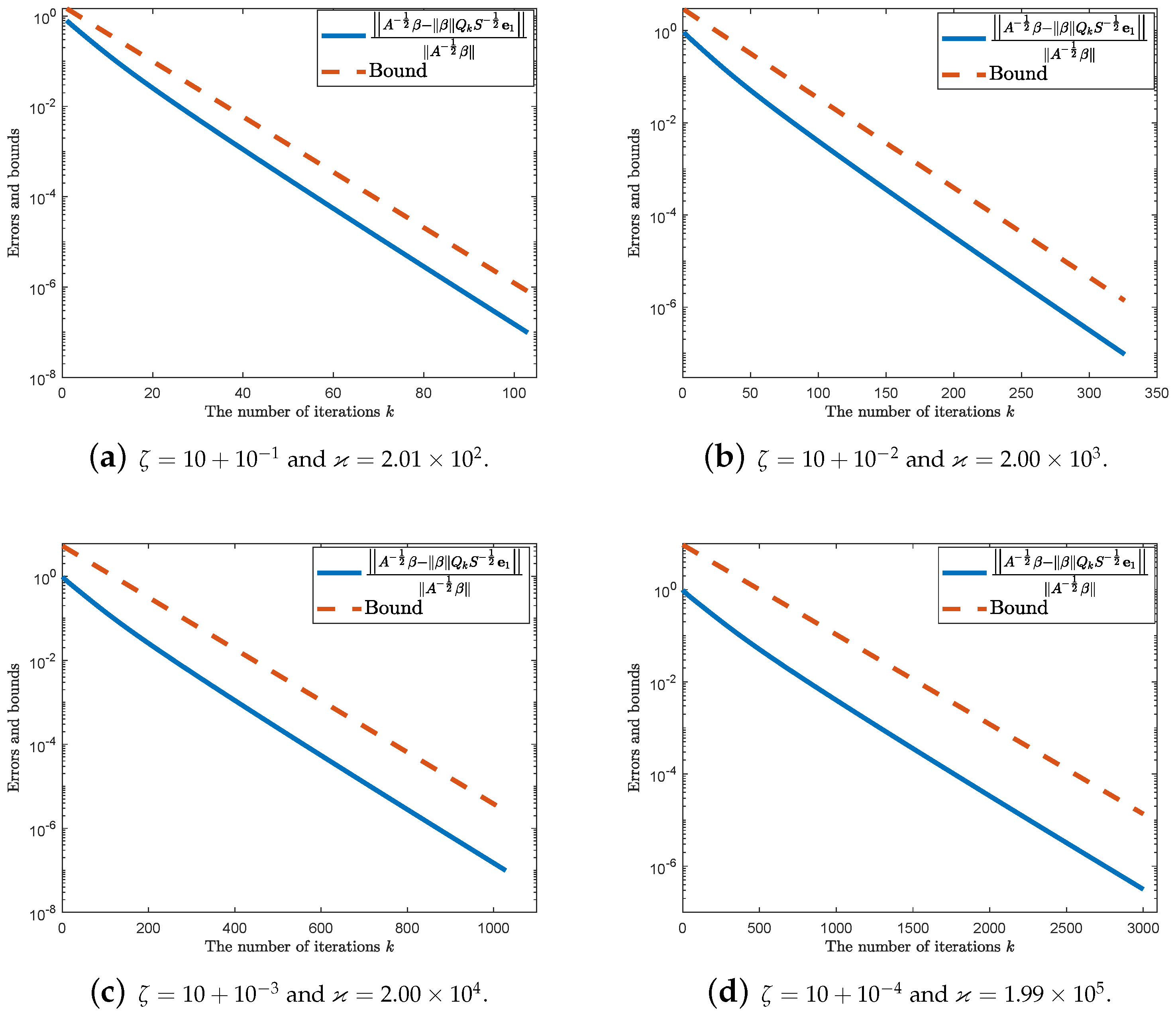
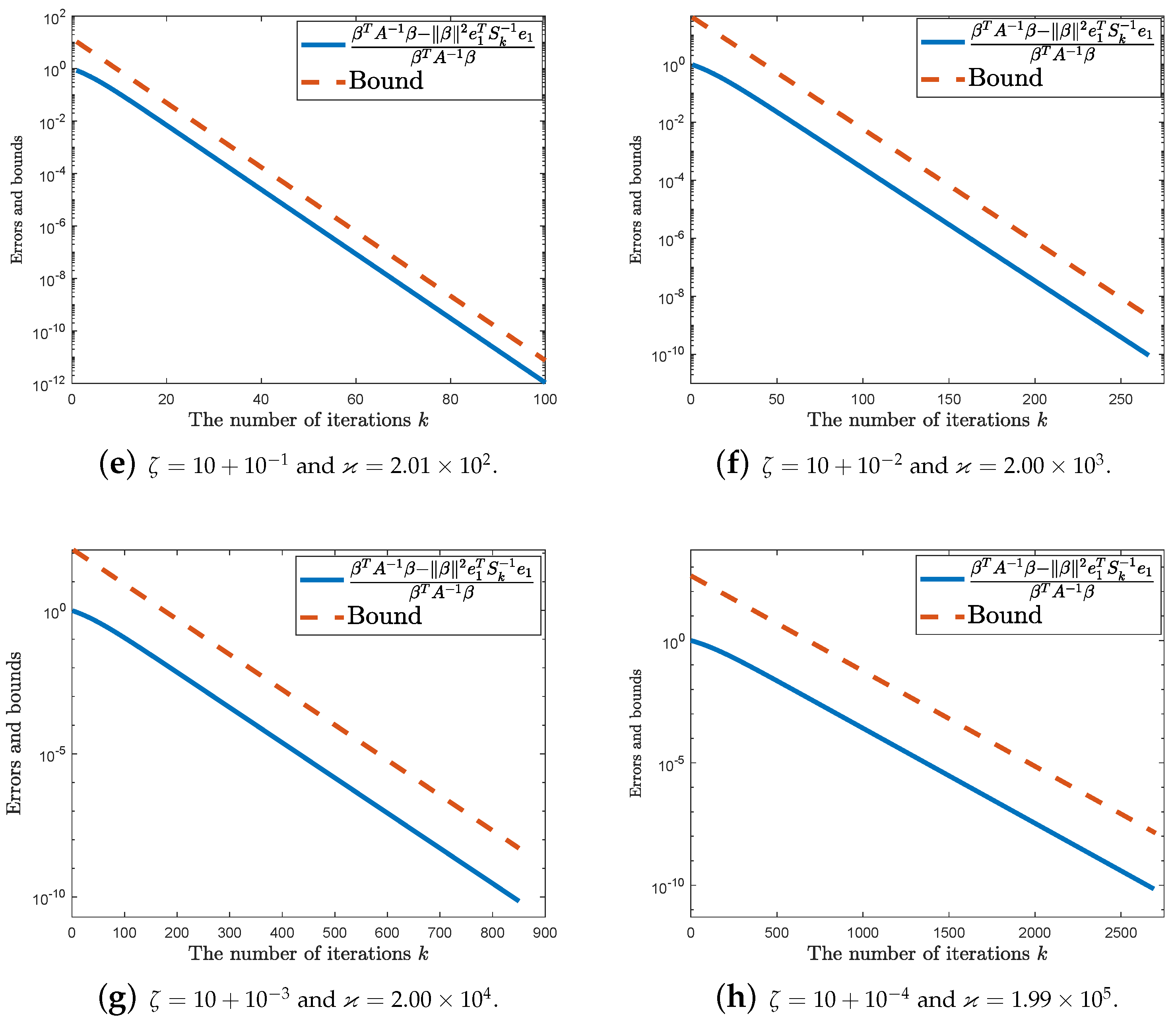
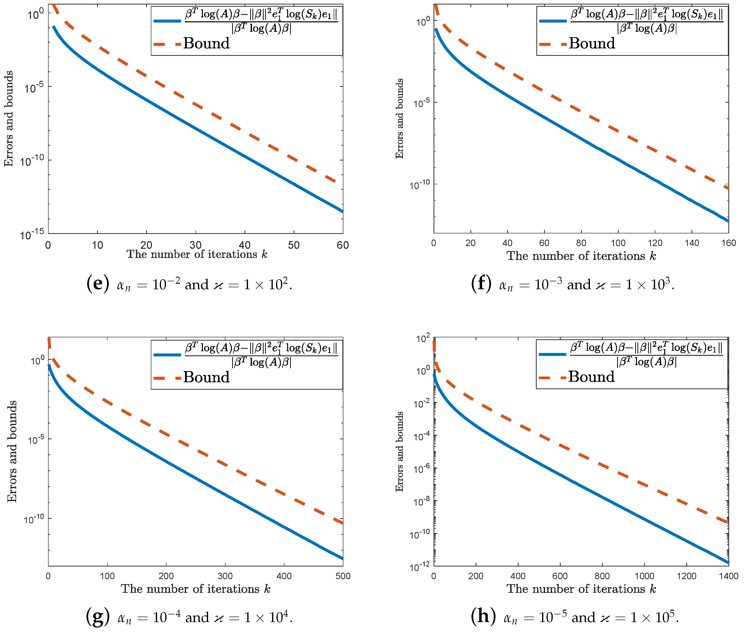
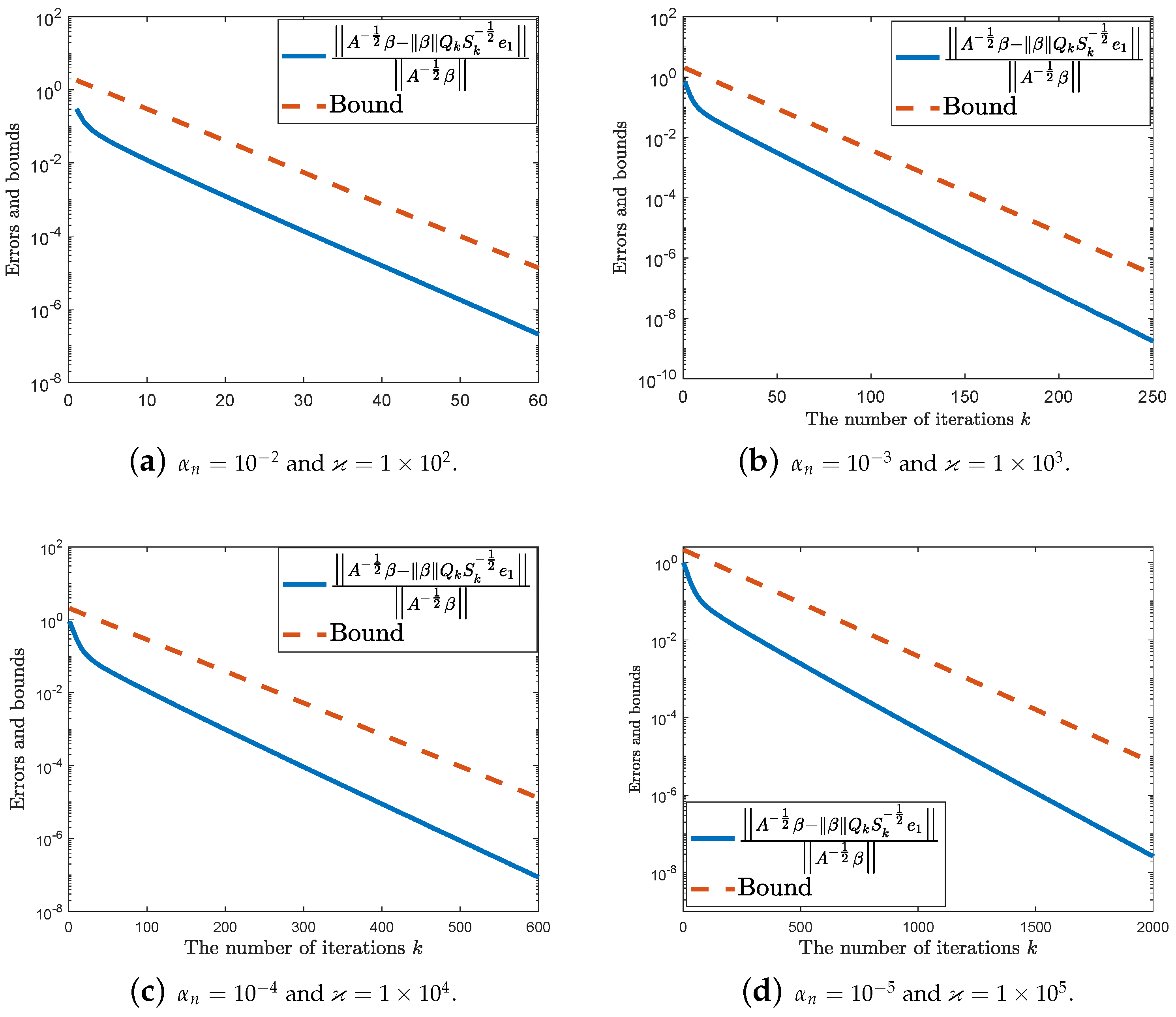
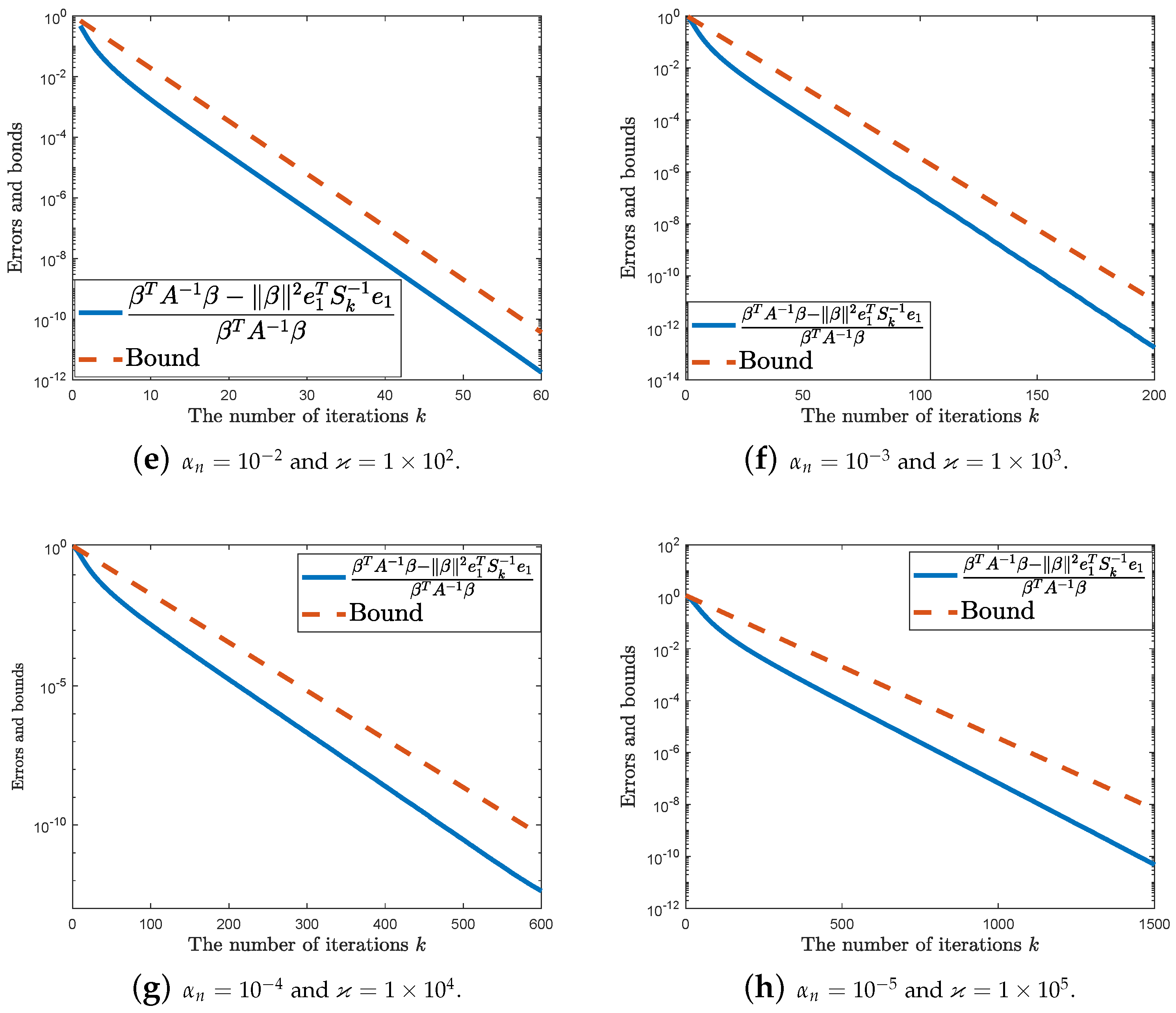
4. Numerical Experiments

We want to show the effectiveness of the bounds provided by (8), (9), (13), and (14) with two examples.

Example 1. 

Let the matrix $B=\mathrm{diag}\left(t_{in}^{[a,b]}\right)$ [31], where

$$t_{in}^{[a,b]}=\left({\displaystyle \frac{b-a}{2}}\right)(t_{in}+({\displaystyle \frac{a+b}{b-a}}\left)\right)\mathrm{with}{t}_{in}=cos{\displaystyle \frac{(2i-1)\pi }{2n}},i=1,2,\dots ,n.$$

Here, $n=5000$, $a=-10,b=10$, and $t_{in}^{[a,b]}$ represents the n-th translated Chebyshev zero node on $[a,b]$. Let

$$A=B+\zeta I,\mathit{\beta }={\displaystyle \frac{\mathit{v}}{\parallel \mathit{v}\parallel }},$$

with

$$\mathit{v}={(11\dots 1)}^T\in {\mathbb{R}}^{5000},\mathrm{and}\zeta >10.$$

The selection of ζ is listed in

Table 1. Example 1: Different values of $\varkappa$ with different choices of $\zeta$.

	$\mathit{\zeta }=10+{10}^{-1}$	$\mathit{\zeta }=10+{10}^{-2}$	$\mathit{\zeta }=10+{10}^{-3}$	$\mathit{\zeta }=10+{10}^{-4}$
$\varkappa$	2.01 × ${10}^2$	2.00 × ${10}^3$	2.00 × ${10}^4$	1.99 × ${10}^5$

.

Example 2. 

Consider the Strakoš matrix

$$A=\mathrm{diag}\left({\left\{{\alpha }_i\right\}}_{i=1}^n\right)\mathrm{with}{\alpha }_i={\alpha }_1+\left({\displaystyle \frac{i-1}{n-1}}\right)({\alpha }_n-{\alpha }_1){\rho }^{n-i},i=1,2,\dots ,n=10000.$$

The distribution of the eigenvalue is controlled by the parameter ρ. We take

$${\alpha }_1=1,\rho =0.99\mathrm{and}\mathit{\beta }={\displaystyle \frac{\mathit{v}}{\parallel \mathit{v}\parallel }},\mathrm{with}\mathit{v}={(11\dots 1)}^T\in {\mathbb{R}}^{10000}$$

in this example. The selection of ${\alpha }_n$ is listed in

Table 2. Example 2: Different values of $\varkappa$ with different choices of ${\alpha }_n$.

	${\mathit{\alpha }}_{\mathit{n}}={10}^{-2}$	${\mathit{\alpha }}_{\mathit{n}}={10}^{-3}$	${\mathit{\alpha }}_{\mathit{n}}={10}^{-4}$	${\mathit{\alpha }}_{\mathit{n}}={10}^{-5}$
$\varkappa$	1 × ${10}^2$	1 × ${10}^3$	1 × ${10}^4$	1 × ${10}^5$

.

So, we obtain different values of $\varkappa$ with different choices of $\zeta$ and ${\alpha }_n$; refer to Table 1 and Table 2. In Figure 1, Figure 2, Figure 3 and Figure 4, we plot the curves of ${ϵ}_1^{\left(k\right)}$, ${ϵ}_2^{\left(k\right)}$, ${ϵ}_3^{\left(k\right)}$, and ${ϵ}_4^{\left(k\right)}$ with different $\varkappa$, as well as the bounds in (8) and (9), respectively. It is obvious to see from Figure 1, Figure 2, Figure 3 and Figure 4 that (i) the iterations increase with the increasing of $\varkappa$, which is consistent with our results (see (8), (9), (13), and (14)); (ii) the convergence rate of ${ϵ}_2^{\left(k\right)}$ is significantly higher than ${ϵ}_1^{\left(k\right)}$ and ${ϵ}_3^{\left(k\right)}$ and slightly higher than that of ${ϵ}_4^{\left(k\right)}$, which is also consistent with our results; (iii) the curves of the bounds in (8), (9), (13), and (14) are almost parallel to the curves of the real values, except for ${ϵ}_3^{\left(k\right)}$ in Example 2 (see Figure 4c,d). That is, our bounds can evaluate the convergence rates of ${ϵ}_1^{\left(k\right)}$, ${ϵ}_2^{\left(k\right)}$, ${ϵ}_3^{\left(k\right)}$, and ${ϵ}_4^{\left(k\right)}$ effectively, in most instances. All these show the effectiveness of the theoretical results proposed in our paper.

5. Concluding Remarks

We established the convergence rates of the Lanczos method for computing $log\left(A\right)\mathit{\beta }$, ${\mathit{\beta }}^{T}log\left(A\right)\mathit{\beta }$, $A^{-{\displaystyle \frac{1}{2}}}\mathit{\beta }$, and ${\mathit{\beta }}^T{A}^{-1}\mathit{\beta }$, as

$$\mathcal{O}\left(k^{-1}{\left({\displaystyle \frac{\sqrt{\varkappa }-1}{\sqrt{\varkappa }+1}}\right)}^k\right),\mathcal{O}\left(k^{-1}{\left({\displaystyle \frac{\sqrt{\varkappa }-1}{\sqrt{\varkappa }+1}}\right)}^{2k-1}\right),\mathcal{O}\left({\left({\displaystyle \frac{\sqrt{\varkappa }-1}{\sqrt{\varkappa }+1}}\right)}^k\right)\mathrm{and}\mathcal{O}\left({\left({\displaystyle \frac{\sqrt{\varkappa }-1}{\sqrt{\varkappa }+1}}\right)}^{2k-1}\right),$$

respectively. Here, A is assumed to be symmetric positive definite. It is not difficult to see that the convergence rate of ${ϵ}_2^{\left(k\right)}$ is significantly higher than ${ϵ}_1^{\left(k\right)}$ and ${ϵ}_3^{\left(k\right)}$ and slightly higher than that of ${ϵ}_4^{\left(k\right)}$. Numerical experiments illustrate the effectiveness of our theoretical results.

The Lanczos method can also be used to compute some other matrix functions, e.g., $exp\left(A\right)\mathit{\beta }$, $A^p\mathit{\beta }$ ($0<p<1$), $sin\left(A\right)\mathit{\beta }$, $cos\left(A\right)\mathit{\beta }$, and so on. The key to convergence analysis is to find the Chebyshev expansion of these functions. Furthermore, our analysis is confined to the scenario where A is symmetric positive definite. The situation is complicated for a nonsymmetric matrix whose eigenvalues are often complex. Therefore, we must resort to the theory of polynomial approximation over complex domains for convergence analysis. Extending this analysis to cases where A is nonsymmetric warrants further investigation. Finally, it is clear from the numerical experiments that the bounds we provide are not sharp enough when the condition number is large, and it is also an interesting question to investigate whether these upper bounds can be improved further.

References

1. Cuchta, T.; Grow, D.; Wintz, N. Discrete matrix hypergeometric functions. J. Math. Anal. Appl. 2023, 518, 126716. [Google Scholar] [CrossRef]
2. Cuchta, T.; Luketic, R. Discrete hypergeometric Legendre polynomials. Mathematics 2021, 9, 2546. [Google Scholar] [CrossRef]
3. Güttel, S. Rational Krylov approximation of matrix functions: Numerical methods and optimal pole selection. GAMM-Mitteilungen 2013, 36, 8–31. [Google Scholar] [CrossRef]
4. Ilic, M.D.; Turner, I.W.; Simpson, D.P. A restarted Lanczos approximation to functions of a symmetric matrix. IMA J. Numer. Anal. 2009, 30, 1044–1061. [Google Scholar] [CrossRef]
5. Ubaru, S.; Chen, J.; Saad, Y. Fast estimation of tr(f(A)) via stochastic Lanczos quadrature. SIAM J. Matrix Anal. Appl. 2017, 38, 1075–1099. [Google Scholar] [CrossRef]
6. Golub, G.H.; Meurant, G. Matrices, Moments and Quadrature with Applications; Princeton University Press: Princeton, NJ, USA, 2009; Volume 30. [Google Scholar]
7. Frommer, A.; Schweitzer, M. Error bounds and estimates for Krylov subspace approximations of Stieltjes matrix functions. BIT Numer. Math. 2015, 56, 865–892. [Google Scholar] [CrossRef]
8. Chen, T.; Hallman, E. Krylov-aware stochastic trace estimation. SIAM J. Matrix Anal. Appl. 2023, 44, 1218–1244. [Google Scholar] [CrossRef]
9. Druskin, V.L.; Knizhnerman, L.A. Error bounds in the simple Lanczos procedure for computing functions of symmetric matrices and eigenvalues. Comput. Math. Math. Phys. 1991, 31, 20–30. [Google Scholar]
10. Frommer, A.; Kahl, K.; Lippert, T.; Rittich, H. 2-norm error bounds and estimates for Lanczos approximations to linear systems and rational matrix functions. SIAM J. Matrix Anal. Appl. 2013, 34, 1046–1065. [Google Scholar] [CrossRef]
11. Higham, N.J. Functions of Matrices: Theory and Computation; SIAM: Philadelphia, PA, USA, 2008. [Google Scholar]
12. Cuchta, T.; Grow, D.; Wintz, N. A dynamic matrix exponential via a matrix cylinder transformation. J. Math. Anal. Appl. 2019, 479, 733–751. [Google Scholar] [CrossRef]
13. Golub, G.H.; Van Loan, C.F. Matrix Computations; Johns Hopkins University Press: Baltimore, MD, USA, 2012. [Google Scholar]
14. Saad, Y. Analysis of Some Krylov Subspace Approximations to the Matrix Exponential Operator. SIAM J. Numer. Anal. 1992, 29, 209–228. [Google Scholar] [CrossRef]
15. Wainwright, M.J.; Jordan, M.I. Log-determinant relaxation for approximate inference in discrete Markov random fields. IEEE Trans. Signal Process. 2006, 54, 2099–2109. [Google Scholar] [CrossRef]
16. Thron, C.; Dong, S.J.; Liu, K.F.; Ying, H.P. Padé-Z2 estimator of determinants. Phys. D-Rev. Part. Fields Gravit. Cosmol. 1998, 57, 1642–1653. [Google Scholar] [CrossRef]
17. Affandi, H.; Fox, E.; Adams, R.; Taskar, B. Learning the parameters of determinantal point process kernels. In Proceedings of the 31st International Conference on Machine Learning, Beijing, China, 21–26 June 2014; pp. 1224–1232. [Google Scholar]
18. Arioli, M.; Loghin, D. Matrix Square-Root Preconditioners for the Steklov-Poincaré Operator; Technical Report RAL-TR-2008-003; Rutherford Appleton Laboratory: Didcot, UK, 2008. [Google Scholar]
19. Tang, J.; Saad, Y. A Probing Method for Computing the Diagonal of the Inverse of a Matrix; Report UMSI–2010–42; Minnesota Supercomputer Institute, University of Minnesota: Minneapolis, MN, USA, 2010. [Google Scholar]
20. Meurant, G. Estimates of the trace of the inverse of a symmetric matrix using the modified Chebyshev algorithms. Numer. Algorithms 2009, 51, 309–318. [Google Scholar] [CrossRef]
21. Bai, Z.; Fahey, M.; Golub, G.H. Some large Scale computation problems. J. Comput. Appl. Math. 1996, 74, 71–89. [Google Scholar] [CrossRef]
22. Bai, Z.; Golub, G.H. Bounds for the trace of the inverse and the determinant of symmetric positive definite matrices. Ann. Numer. Math. 1997, 4, 29–38. [Google Scholar]
23. Dong, S.J.; Liu, K.F. Stochastic estimation with Z2 noise. Phys. Lett. B 1994, 328, 130–136. [Google Scholar] [CrossRef]
24. Ortner, B.; Krauter, A.R. Lower bounds for the determinant and the trace of a class of Hermitian matrices. Linear Algebra Its Appl. 1996, 236, 147–180. [Google Scholar] [CrossRef]
25. Brezinski, C.; Fika, P.; Mitrouli, M. Moments of a linear operator, with applications to the trace of the inverse of matrices and the solution of equations. Numer. Linear Algebra Appl. 2012, 19, 937–953. [Google Scholar] [CrossRef]
26. Wu, L.; Laeuchli, J.; Kalantzis, V.; Stathopoulos, A.; Gallopoulos, E. Estimating the trace of the matrix inverse by interpolating from the diagonal of an approximate inverse. J. Comput. Phys. 2016, 326, 828–844. [Google Scholar] [CrossRef]
27. Beals, R.; Wong, R. Special Functions and Orthogonal Polynomials; Cambridge University Press: Cambridge, UK, 2016. [Google Scholar]
28. Olver, F.; Lozier, D.; Boisvert, R.; Clark, C. The NIST Handbook of Mathematical Functions; Cambridge University Press: New York, NY, USA, 2010. [Google Scholar]
29. Bernstein, S.N. Sur l, ordre de la meilleure approximation des fonctions continues par les polynômes de degré donné. R. Acad. Med. Belg. 1912, 4, 1–104. [Google Scholar]
30. Zhan, X. Matrix Inequalities; Springer: Berlin/Heidelberg, Germany, 2002. [Google Scholar]
31. Zhang, L.; Shen, C.; Li, R. On the generalized Lanczos trust-region method. SIAM J. Optim. 2017, 27, 2110–2142. [Google Scholar] [CrossRef]
Figure 1. Example 1: Lines correspond to ϵ 1 ( k ) and ϵ 2 ( k ) ; refer to Theorem 1.
Axioms 13 00764 g001aAxioms 13 00764 g001b
Figure 2. Example 1: Lines correspond to ϵ 3 ( k ) and ϵ 4 ( k ) ; refer to Theorems 2 and 3.
Axioms 13 00764 g002aAxioms 13 00764 g002b
Figure 3. Example 2: Lines correspond to ϵ 1 ( k ) and ϵ 2 ( k ) ; refer to Theorem 1.
Axioms 13 00764 g003aAxioms 13 00764 g003b
Figure 4. Example 2: Lines correspond to ϵ 3 ( k ) and ϵ 4 ( k ) ; refer to Theorems 2 and 3.
Axioms 13 00764 g004aAxioms 13 00764 g004b