A Global Method for Approximating Caputo Fractional Derivatives—An Application to the Bagley–Torvik Equation

Abstract

In this paper, we propose a global numerical method for approximating Caputo fractional derivatives of order $\alpha$$\left(D^{\alpha }f\right)\left(y\right)=\frac{1}{\Gamma (m-\alpha )}{\int }_0^y{(y-x)}^{m-\alpha -1}{f}^{\left(m\right)}\left(x\right)dx,y>0$, with $m-1<\alpha \le m,m\in \mathbb{N}.$ The numerical procedure is based on approximating $f^{\left(m\right)}$ by the m-th derivative of a Lagrange polynomial, interpolating f at Jacobi zeros and some additional nodes suitably chosen to have corresponding logarithmically diverging Lebsegue constants. Error estimates in a uniform norm are provided, showing that the rate of convergence is related to the smoothness of the function f according to the best polynomial approximation error and depending on order $\alpha$. As an application, we approximate the solution of a Volterra integral equation, which is equivalent in some sense to the Bagley–Torvik initial value problem, using a Nyström-type method. Finally, some numerical tests are presented to assess the performance of the proposed procedure.

1. Introduction

The paper considers the numerical evaluation of Caputo fractional derivatives of order $\alpha$ of a given function f, i.e.,

$$\begin{array}{ccc}\hfill \left(D^{\alpha }f\right)\left(y\right)& =& \frac{1}{\Gamma (m-\alpha )}{\int }_0^y{(y-x)}^{m-\alpha -1}{f}^{\left(m\right)}\left(x\right)dx,y>0,\hfill \\ & & m-1<\alpha \le m,m\in \mathbb{N}.\hfill \end{array}$$

Fixing the case $y\in [0,1]$, the numerical procedure is based on approximating $f^{\left(m\right)}\sim L_{n,r,s}^{\left(m\right)}(v^{\gamma ,\delta },f)$, where the polynomial $L_{n,r,s}(v^{\gamma ,\delta },f)$ interpolates f at the zeros of the n-th orthogonal polynomial $p_n^{\gamma ,\delta }$ with respect to the Jacobi weight $v^{\gamma ,\delta }\left(y\right)={(1-y)}^{\gamma }{y}^{\delta },\gamma ,\delta >-1$ and $r+s$ additional nodes. According to the “additional method nodes” [1], the latter are chosen in such a way that the norm of the operator $L_{n,r,s}\left(v^{\gamma ,\delta }\right):C^0\left([0,1]\right)\to C^0\left([0,1]\right)$ diverges as $logn$.

Fractional calculus has a long history, but only over the last few decades has its usefulness in applications become more evident. Indeed, fractional derivatives have been occurring more and more frequently in many physical and engineering problems, including diffusion processes [2,3,4,5], signal processing [6], and modeling of viscoelastic materials [7,8,9,10]. For this reason, efficient and reliable techniques for computing $D^{\alpha }f$ are needed. Several textbooks and papers (see, e.g., [4,11,12,13,14,15,16,17]) have been published dealing with various aspects of fractional calculus, ranging from its history to analytical and numerical results to possible applications. In addition, several papers dealing with numerical methods for solving differential equations of fractional order are available in the literature; among others, we mention [18,19,20,21,22,23,24,25,26] and the references therein. In particular, accurate classification and description of some numerical approximations proposed for the most frequently utilized fractional integrals and derivatives have been presented in [12,27].

One of the main advantages of the global approach we discuss here is the rate of convergence, which is related to the smoothness of the function f according to the best polynomial approximation error and depending on the order $\alpha$. Such estimates improve upon those stated in [13], and allow us to obtain finer results with fewer function evaluations than those required by local piecewise approximants (see, e.g., [28]). Furthermore, for any fractional derivative, the majority of methods for evaluating different functions, i.e., those at the Jacobi zeros, remain unchanged regardless of the fractional order $\alpha$.

As an application of the above-described numerical procedure, we propose a new Nyström-type method for solving the Bagley–Torvik initial value problem [7,8] and approximating the solution of the equivalent Volterra integral equation. We prove the convergence of the Nyström method, providing error estimates in the uniform norm. Such a numerical method leads to solving a system of linear equations with a dimension that is just the number of the function’s evaluations.

The rest of this paper is outlined as follows: Section 2 contains some basic definitions and preliminary results about the polynomial tool that we employ and a few properties of the fractional derivatives useful for our aims; Section 3 describes the method that we propose, along with error estimates, computational details, and some numerical tests; Section 4 is dedicated to the application of the introduced numerical scheme to approximate the solution of the Bagley–Torvik initial value problem, along with error estimates and some numerical tests; finally, Section 5 states the proofs of the main results.

2. Preliminary Results

In the sequelae, we denote by $\mathcal{C}$ any positive constant having different meanings at different occurrences. The notation $\mathcal{C}\ne \mathcal{C}(a,b,\dots )$ is used to underline that $\mathcal{C}$ does not depend on $a,b,\dots$. Moreover, where $A,B>0$ are quantities depending on some parameters, writing $A\sim B,$ should be understood as indicating the existence of a constant $\mathcal{C}\ne \mathcal{C}(A,B)$ such that ${\mathcal{C}}^{-1}B\le A\le \mathcal{C}B.$ Finally, ${\mathbb{P}}_n$ is used to denote the space of algebraic polynomials of degree less than or equal to n.

2.1. Function Spaces

For any $0<T<\infty$, $C^0\left([0,T]\right)$ is the space of all continuous functions, and is equipped with the uniform norm ${\parallel f\parallel }_{\infty }={max}_{x\in [0,T]}\left|f\left(x\right)\right|.$ Let $E_n\left(f\right)$ be the best polynomial approximation error in $C^0\left([0,T]\right)$, i.e.,

$$E_n\left(f\right)=\underset{P\in {\mathbb{P}}_n}{inf}{\parallel f-P\parallel }_{\infty },$$

and characterizing $C^0\left([0,T]\right)$, i.e.,

$$\underset{n}{lim}{E}_n\left(f\right)=0⟺f\in C^0\left([0,T]\right).$$

As usual, for any integer $q\ge 1$, $C^q\left([0,T]\right)$ denotes the space of at least q times differentiable functions such that the q-th derivative $f^{\left(q\right)}\in C^0\left([0,T]\right)$, and is equipped with the norm

$${\parallel f\parallel }_{q,\infty }=\underset{0\le i\le q}{max}{\parallel f^{\left(i\right)}\parallel }_{\infty }.$$

We use $\omega (f,\delta )$ to denote the ordinary modulus of continuity of f, recalling the following Jackson inequality (see e.g., (5.1) in [29]):

$$E_n\left(f\right)\le \mathcal{C}\omega \left(f,\frac{T}{n}\right),\forall f\in C^0\left([0,T]\right),\mathcal{C}\ne \mathcal{C}(n,f).$$

(1)

The Hölder space $H_M^{\mu }$ on $[0,T]$ with $0<\mu \le 1,M>0$ is characterized as

$$\forall f\in C^0\left([0,T]\right):\omega (f,\delta )\le M{\delta }^{\mu }⟺f\in H_M^{\mu }.$$

For smoother functions, we recall that for any $f\in C^q\left([0,T]\right)$ [30]

$$E_n\left(f\right)\le \frac{\mathcal{C}}{n^q}{E}_{n-q}\left(f^{\left(q\right)}\right)\le \mathcal{C}\frac{{\parallel f\parallel }_{q,\infty }}{n^q},\mathcal{C}\ne \mathcal{C}(f,n)$$

(2)

and that for $f\in C^{q+\mu }\left([0,T]\right)$ (i.e., $f^{\left(q\right)}\in H_M^{\mu }$) (see Section 5.1.5 in [29])

$$E_n\left(f\right)\le \mathcal{C}M{\left(\frac{T}{n}\right)}^{q+\mu },\mathcal{C}\ne \mathcal{C}(f,n).$$

(3)

In what follows, in the case of $T=1$ we use the simpler notation $C^q:=C^q\left([0,1]\right)q\ge 0$ and $C^{q+\mu }:=C^{q+\mu }\left([0,1]\right).$

2.2. Optimal Interpolation Processes

Consider the Jacobi weight $v^{\gamma ,\delta }\left(x\right)={(1-x)}^{\gamma }{x}^{\delta },\gamma ,\delta >-1,x\in (0,1)$ and denote by ${\left\{p_n\left(v^{\gamma ,\delta }\right)\right\}}_{n\ge 0}$ the corresponding system of orthonormal polynomials with positive leading coefficients. Let $x_{n,j}^{\gamma ,\delta },j=1,\dots ,n,$ be the roots of $p_n\left(v^{\gamma ,\delta }\right)$ and let ${\lambda }_{n,j}^{\gamma ,\delta }$ be the Christoffel numbers

$${\lambda }_{n,j}^{\gamma ,\delta }={\left(\sum _{i=0}^{n-1}{p}_i^2(v^{\gamma ,\delta },x_{n,j}^{\gamma ,\delta })\right)}^{-1},j=1,2,\dots ,n.$$

For a given function $f\in C^0$, let ${\mathcal{L}}_n^{\gamma ,\delta }\left(f\right)\in {\mathbb{P}}_{n-1}$ be the Lagrange polynomial interpolating f at the zeros of $p_n\left(v^{\gamma ,\delta }\right),$ i.e.,

$${\mathcal{L}}_n^{\gamma ,\delta }(f,x)=\sum _{i=1}^n{l}_{n,i}(v^{\gamma ,\delta },x)f\left(x_{n,i}^{\gamma ,\delta }\right),l_{n,i}(v^{\gamma ,\delta },x)=\frac{p_n(v^{\gamma ,\delta },x)}{p_n^{\prime }(v^{\gamma ,\delta },x_{n,i}^{\gamma ,\delta })(x-x_{n,i}^{\gamma ,\delta })},$$

and also

$$l_{n,i}(v^{\gamma ,\delta },x)={\lambda }_{n,i}^{\gamma ,\delta }\sum _{k=0}^{n-1}{p}_k(v^{\gamma ,\delta },x)p_k(v^{\gamma ,\delta },x_{n,i}^{\gamma ,\delta }).$$

(4)

Denoting by $\parallel {\mathcal{L}}_n^{\gamma ,\delta }{\parallel }_{\infty }$ the norm of the operator ${\mathcal{L}}_n^{\gamma ,\delta }:C^0\to C^0$, i.e., the n-th Lebesgue constant, it is well known (see, e.g., Chapter 4 in [31]) that $\{\parallel {\mathcal{L}}_n^{\gamma ,\delta }{\parallel \}}_n$ growing at least as $logn$ plays an essential role in the study of the convergence of the Lagrange polynomial, as

$$\parallel f-{\mathcal{L}}_n^{\gamma ,\delta }{\left(f\right)\parallel }_{\infty }\le (1+\parallel {\mathcal{L}}_n^{\gamma ,\delta }\parallel )E_{n-1}{\left(f\right)}_{\infty }.$$

In view of a classical result by Szëgo, the following behavior arises:

$$\parallel {\mathcal{L}}_n^{\gamma ,\delta }{\parallel }_{\infty }\sim \left\{\begin{array}{cc}logn,\hfill & -1<\gamma ,\delta \le -\frac{1}{2}\hfill \\ n^{max\{\gamma ,\delta \}+\frac{1}{2}},\hfill & \mathrm{otherwise}.\hfill \end{array}\right.$$

For instance, the Lebesgue constants related to the Legendre weight ($\gamma =\delta =0$) or the Chebyshev weight of the second kind ($\gamma =\delta =\frac{1}{2}$) algebraically diverge, as $n\to \infty$.

On the other hand, in [1] it was proved that by suitably modifying the above interpolation process, the corresponding Lebesgue constants also behave as $logn$ in the case of $\gamma >-1/2$ or $\delta >-1/2$.

To describe the modified process, given two positive integers r and s, let

$$y_j=\frac{j}{s}{x}_{n,1}^{\gamma ,\delta },j=0,\dots ,s-1,z_j=x_{n,n}^{\gamma ,\delta }+\frac{j}{r}(1-x_{n,n}^{\gamma ,\delta }),j=1,\dots ,r,$$

and set

$$t_i:=\left\{\begin{array}{cc}{y}_{i-1}\hfill & i=1,\dots ,s,\hfill \\ x_{n,i-s}^{\gamma ,\delta }\hfill & i=s+1,\dots ,s+n,\hfill \\ z_{i-s-n}\hfill & i=s+n+1,\dots ,s+n+r.\hfill \end{array}\right.$$

(5)

Let $L_{n,r,s}(v^{\gamma ,\delta },f)$ be the polynomial interpolating f at the nodes ${\left\{t_i\right\}}_{i=1}^{n+r+s}$, i.e.,

$$L_{n,r,s}(v^{\gamma ,\delta },f)\in {\mathbb{P}}_{n+r+s-1},L_{n,r,s}(v^{\gamma ,\delta },f,t_i)=f\left(t_i\right),i=1,2,\dots ,n+r+s.$$

The following result proved in [1] shows how the sequence $\left\{L_{n,r,s}(v^{\gamma ,\delta },f)\right\}$ can be a useful tool for simultaneously approximating f and its derivatives in the uniform norm.

Theorem 1. 

Let $L_{n,r,s}(v^{\gamma ,\delta },f)$ be the polynomial defined by (9), with $f\in C^q,q\ge 0,$ and let h be an integer s.t. $0\le h\le q.$ If

$$\begin{array}{c}\frac{(h+\gamma )}{2}+\frac{1}{4}\le r\le \frac{(h+\gamma )}{2}+\frac{5}{4}\\ \\ \frac{(h+\delta )}{2}+\frac{1}{4}\le s\le \frac{(h+\delta )}{2}+\frac{5}{4},\end{array}$$

(6)

then for $n\ge 4q+5$ we have

$$\parallel f^{\left(h\right)}-L_{n,r,s}^{\left(h\right)}(v^{\gamma ,\delta },f){\parallel }_{\infty }\le \mathcal{C}\frac{E_{n-q}\left(f^{\left(q\right)}\right)}{n^{q-h}}logn$$

(7)

with $\mathcal{C}\ne \mathcal{C}(n,f)$.

Remark 1. 

For any $q\ge 0$, under assumptions (6), the following estimate holds [1]:

$$\parallel L_{n,r,s}\left(v^{\gamma ,\delta }\right){\parallel }_{q,\infty }:=\underset{{\parallel f\parallel }_{q,\infty }=1}{sup}{\parallel L_{n,r,s}(v^{\gamma ,\delta },f)\parallel }_{q,\infty }\le \mathcal{C}logn,\mathcal{C}\ne \mathcal{C}\left(n\right).$$

(8)

Remark 2. 

Given (2) and (3), the following error estimates follow from (7):

$$\parallel f^{\left(h\right)}-L_{n,r,s}^{\left(h\right)}(v^{\gamma ,\delta },f){\parallel }_{\infty }\le \mathcal{C}\left\{\begin{array}{cc}\frac{{\parallel f\parallel }_{q,\infty }}{n^{q-h}}logn,\hfill & f\in C^q\hfill \\ \\ \frac{M}{n^{q+\mu -h}}logn,\hfill & f\in C^{q+\mu }\hfill \end{array}\right.$$

with $\mathcal{C}\ne \mathcal{C}(n,f)$.

Remark 3. 

The procedure described above is known as the ”method of additional nodes”, and has been used by several authors in different contexts. The sequence ${\left\{L_{n,r,s}(v^{\gamma ,\delta },f)\right\}}_n$ was introduced in [1] in the natural interval $(-1,1)$, where the Jacobi zeros are, for the simultaneous approximation of f and its derivatives in the uniform norm. The case of $\gamma =\delta =-1/2$ has been treated in [32]. For a short history of the additional nodes method, the interested reader can consult [31] (p. 264). We highlight that the previous interpolation process is very useful for simultaneously approximating the function f and its derivatives by using only the samples of f at the points ${\left\{t_i\right\}}_{i=1}^{n+r+s}.$

2.3. Computational Details

The interpolating polynomial $L_{n,r,s}(v^{\gamma ,\delta },f)$ can be represented as

$$L_{n,r,s}(v^{\gamma ,\delta },f,x)=\sum _{k=1}^{r+n+s}{\ell }_{n,k}(v^{\gamma ,\delta },x)f\left(t_k\right),{\ell }_{n,k}(v^{\gamma ,\delta },x)=\underset{i\ne k}{\prod _{i=1}^{r+n+s}}\frac{x-t_i}{t_k-t_i};$$

(9)

equivalently, setting

$$A_s\left(x\right)=\prod _{i=1}^s(x-y_{i-1}),B_r\left(x\right)=\prod _{i=1}^r(x-z_i),$$

it takes the form

$$\begin{array}{ccc}\hfill L_{n,r,s}(v^{\gamma ,\delta },f,x)& =& A_s\left(x\right)B_r\left(x\right)\sum _{k=1}^n{l}_{n,k}(v^{\gamma ,\delta },x)\frac{f\left(x_{n,k}^{\gamma ,\delta }\right)}{A_s\left(x_{n,k}^{\gamma ,\delta }\right)B_r\left(x_{n,k}^{\gamma ,\delta }\right)}\hfill \\ & +& A_s\left(x\right)p_n(v^{\gamma ,\delta },x)\sum _{k=1}^r\frac{f\left(z_k\right)}{A_s\left(z_k\right)p_n(v^{\gamma ,\delta },z_k)}\prod _{i=1,i\ne k}^r\frac{x-z_i}{z_k-z_i}\hfill \\ & +& B_r\left(x\right)p_n(v^{\gamma ,\delta },x)\sum _{k=1}^s\frac{f\left(y_{k-1}\right)}{B_r\left(y_{k-1}\right)p_n(v^{\gamma ,\delta },y_{k-1})}\prod _{i=1,i\ne k}^s\frac{x-y_{i-1}}{y_{k-1}-y_{i-1}}.\hfill \end{array}$$

(10)

To compute the derivatives of the polynomials ${\ell }_{n,k}(v^{\gamma ,\delta },x)$ in (9), we can set

$$S_{j,k}\left(x\right)=\underset{i\ne k}{\sum _{i=1}^{r+n+s}}\frac{1}{{(x-t_i)}^j},j\in \mathbb{N},j\ge 1,$$

(11)

by the Leibnitz rule derivative to easily obtain

$$\begin{array}{ccc}\hfill {\ell }_{n,k}^{\prime }(v^{\gamma ,\delta },x)& =& {\ell }_{n,k}(v^{\gamma ,\delta },x)S_{1,k}\left(x\right),\hfill \\ \hfill & \hfill & \hfill \\ \hfill {\ell }_{n,k}^{(h+1)}(v^{\gamma ,\delta },x)& =& \sum _{j=0}^h\frac{{(-1)}^{j}h!}{(h-j)!}{\ell }_{n,k}^{(h-j)}(v^{\gamma ,\delta },x)S_{j+1,k}\left(x\right),h\ge 1.\hfill \end{array}$$

(12)

In the special case with $r=s=1$ and selecting $y_0=0,z_1=1$, the polynomial in (10) takes the form

$$\begin{array}{ccc}\hfill L_{n,1,1}(v^{\gamma ,\delta },f,x)& =& x(x-1)\sum _{k=1}^n{l}_{n,k}(v^{\gamma ,\delta },x)\frac{f\left(x_{n,k}^{\gamma ,\delta }\right)}{x_{n,k}^{\gamma ,\delta }(x_{n,k}^{\gamma ,\delta }-1)}\hfill \\ & +& p_n(v^{\gamma ,\delta },x)\left[\frac{x}{p_n(v^{\gamma ,\delta },1)}f\left(1\right)-\frac{(x-1)}{p_n(v^{\gamma ,\delta },0)}f\left(0\right)\right]\hfill \end{array}$$

(13)

and

$$\begin{array}{ccc}\hfill L_{n,1,1}^{\left(m\right)}(v^{\gamma ,\delta },f,x)& =& \sum _{k=1}^n\frac{f\left(x_{n,k}^{\gamma ,\delta }\right)}{x_{n,k}^{\gamma ,\delta }(x_{n,k}^{\gamma ,\delta }-1)}\left(m(m-1)l_{n,k}^{(m-2)}(v^{\gamma ,\delta },x)+m(2x-1)l_{n,k}^{(m-1)}(v^{\gamma ,\delta },x)\right.\hfill \\ & +& \left.x(x-1)l_{n,k}^{\left(m\right)}(v^{\gamma ,\delta },x)\right)+\frac{m{p}_n^{(m-1)}(v^{\gamma ,\delta },x)+x{p}_n^{\left(m\right)}(v^{\gamma ,\delta },x)}{p_n(v^{\gamma ,\delta },1)}f\left(1\right)\hfill \\ & -& \frac{m{p}_n^{(m-1)}(v^{\gamma ,\delta },x)+(x-1)p_n^{\left(m\right)}(v^{\gamma ,\delta },x)}{p_n(v^{\gamma ,\delta },0)}f\left(0\right),\hfill \end{array}$$

(14)

where

$$l_{n,k}^{\left(i\right)}(v^{\gamma ,\delta },x)={\lambda }_{n,k}\left(v^{\gamma ,\delta }\right)\sum _{j=i}^{n-1}{p}_j^{\left(i\right)}(v^{\gamma ,\delta },x)p_j(v^{\gamma ,\delta },x_{n,k}\left(v^{\gamma ,\delta }\right)),i=1,2,\dots ,n-1,$$

$$p_n^{\left(i\right)}(v^{\gamma ,\delta },x)=\frac{\Gamma (n+i+\gamma +\delta +1)}{2^i\Gamma (n+\gamma +\delta +2)}{p}_{n-i}(v^{\gamma +i,\delta +i},x),i=1,2,\dots ,n,$$

and $\Gamma$ denotes Euler’s Gamma function.

We conclude by recalling that ${(x_{n,j}^{\gamma ,\delta },{\lambda }_{n,j}^{\gamma ,\delta })}_{j=1,\dots ,n}$ are related to the zeros and Christoffel numbers ${(X_{n,j}^{\gamma ,\delta },{\Lambda }_{n,j}^{\gamma ,\delta })}_{j=1,\dots ,n}$, which are defined in $(-1,1)$ with respect to the weight ${(1-x)}^{\gamma }{(1+x)}^{\delta }$ through the relations

$$x_{n,j}^{\gamma ,\delta }=\frac{X_{n,j}^{\gamma ,\delta }+1}{2},{\lambda }_{n,j}^{\gamma ,\delta }=\frac{1}{2^{\gamma +\delta }}{\Lambda }_{n,j}^{\gamma ,\delta },j=1,2,\dots ,n,$$

In addition, ${(X_{n,j}^{\gamma ,\delta },{\Lambda }_{n,j}^{\gamma ,\delta })}_{j=1,\dots ,n}$ are computed by the Golub and Welsch algorithm [33]. Relying on a modification of the QR–method, this yields the nodes and weights by computing the eigenvalues of the Jacobi matrix and the first row of the associated eigenvector matrix.

2.4. Caputo Fractional Derivatives

We recall the definition of Caputo’s fractional derivative of order $\alpha >0.$ With $m-1<\alpha <m$ [15], it is defined as

$$\left(D^{\alpha }f\right)\left(y\right)=J^{m-\alpha }{\left(\frac{d}{dy}\right)}^{m}f\left(y\right),$$

(15)

where

$$J^{\alpha }f\left(y\right)=\frac{1}{\Gamma \left(\alpha \right)}{\int }_0^y{(y-s)}^{\alpha -1}f\left(s\right)ds$$

is the Riemann–Liouville fractional integral operator of order $\alpha >0$. From this definition, it follows that

$$\left(D^{\alpha }f\right)\left(y\right)=\frac{1}{\Gamma (m-\alpha )}{\int }_0^y{(y-x)}^{m-\alpha -1}{f}^{\left(m\right)}\left(x\right)dx,y>0.$$

(16)

For $m\to \alpha$, Caputo’s fractional derivative is defined as

$$\left(D^{m}f\right)\left(y\right)=f^{\left(m\right)}\left(y\right).$$

In what follows, we will consider the case of functions $f\in C^0\left([0,T]\right)$ for fixed $T>0$.

For $0<\alpha <1$, it is known that the operator $J^{\alpha }:C^0\left([0,T]\right)\to H_M^{\alpha }$ is linear and bounded and that $J^{\alpha }:C^0\left([0,T]\right)\to C^0\left([0,T]\right)$ is compact (see, e.g., [19,34,35,36]; see also [37] (Lemma 6.2)). As a consequence, taking into account definition (15) of $D^{\alpha }f$, it follows that, for any $f\in C^m\left([0,T]\right),m\ge 0$,

$$D^{\alpha }f\in H_M^{m-\alpha }.$$

(17)

3. Approximation of Caputo Fractional Derivatives

In this section, we describe the proposed method for numerically evaluating $\left(D^{\alpha }f\right),$ under the assumption $f\in C^m$ for the case of $y\in [0,1].$ With $L_{n,r,s}(v^{\gamma ,\delta },f,x)$ as defined in (9), in view of the “fine” results about the simultaneous approximation evidenced by (7) and (8), we propose using $f^{\left(m\right)}\sim L_{n,r,s}^{\left(m\right)}(v^{\gamma ,\delta },f)$ to obtain

$$\begin{array}{ccc}\hfill \left(D_n^{\alpha }f\right)\left(y\right)& =& \frac{1}{\Gamma (m-\alpha )}{\int }_0^y{(y-x)}^{m-\alpha -1}{L}_{n,r,s}^{\left(m\right)}(v^{\gamma ,\delta },f,x)dx\hfill \\ & =& \frac{1}{\Gamma (m-\alpha )}\sum _{k=1}^{r+n+s}f\left(t_k\right){\int }_0^y{(y-x)}^{m-\alpha -1}{\ell }_{n,k}^{\left(m\right)}(v^{\gamma ,\delta },x)dx\hfill \end{array}$$

(18)

$$\begin{array}{ccc}& =& \frac{y^{m-\alpha }}{\Gamma (m-\alpha )}\sum _{k=1}^{r+n+s}f\left(t_k\right){\int }_0^1{\ell }_{n,k}^{\left(m\right)}(v^{\gamma ,\delta },ty)v^{m-\alpha -1,0}\left(t\right)dt.\hfill \end{array}$$

(19)

By the Gauss–Jacobi rule of order $N=\lceil \frac{n+r+s-m}{2}\rceil$ with respect to the weight $v^{m-\alpha -1,0}$, with $x_{N,i}^{m-\alpha -1,0}$ and ${\lambda }_{N,i}^{m-\alpha -1,0}$, $i=1,\dots ,N$ as the corresponding knots and Christoffel numbers, respectively, we obtain

$$\begin{array}{ccc}\hfill \left(D_n^{\alpha }f\right)\left(y\right)& =& \frac{y^{m-\alpha }}{\Gamma (m-\alpha )}\sum _{k=1}^{r+n+s}f\left(t_k\right)\sum _{i=1}^N{\ell }_{n,k}^{\left(m\right)}(v^{\gamma ,\delta },x_{N,i}^{m-\alpha -1,0}y){\lambda }_{N,i}^{m-\alpha -1,0}\hfill \end{array}$$

and hence

$$\begin{array}{ccc}\hfill \left(D_n^{\alpha }f\right)\left(y\right)& =:& \frac{y^{m-\alpha }}{\Gamma (m-\alpha )}\sum _{k=1}^{r+n+s}f\left(t_k\right)d_k^m\left(y\right),\hfill \end{array}$$

(20)

where

$$d_k^m\left(y\right)=\sum _{i=1}^N{\ell }_{n,k}^{\left(m\right)}(v^{\gamma ,\delta },x_{N,i}^{m-\alpha -1,0}y){\lambda }_{N,i}^{m-\alpha -1,0}.$$

Now, we state a result dealing with the convergence of the proposed rule and providing some upper bounds of the quadrature error.

Theorem 2. 

With the assumptions in (6) satisfied, for any $f\in C^q$, $q\ge m,$

$$\parallel D^{\alpha }f-D_n^{\alpha }{f\parallel }_{\infty }\le \mathcal{C}\frac{E_{n-q}\left(f^{\left(q\right)}\right)}{n^{q-m}}logn,\mathcal{C}\ne \mathcal{C}(n,f),$$

(21)

and for $f\in C^{q+\mu }$, $q\ge m,0<\mu \le 1,$

$$\parallel D^{\alpha }f-D_n^{\alpha }{f\parallel }_{\infty }\le \mathcal{C}\frac{M}{n^{q+\mu -m}}logn,\mathcal{C}\ne \mathcal{C}(n,f).$$

(22)

Theorem 2 ensures that the rule uniformly converges to $D^{\alpha }f$ with a rate depending on the smoothness of f and on $m=\lceil \alpha \rceil$, with $\alpha$ as the order of the fractional derivative.

Remark 4. 

In [13], the authors proposed approximating $f^{\left(m\right)}$ using the m-th derivative of the Gauss–Lobatto zeros-based interpolating polynomial $P_{n+2}(v^{0,0},f)$, which in this case coincides with the polynomial $L_{n,1,1}(v^{0,0},f)$. However, the final error estimate that they derived for $f\in C^q,q\ge 2m,$ (see Remark 5.2 in [13]) was

$$\parallel D^{\alpha }f-D^{\alpha }{P}_{n+2}(v^{0,0},f){\parallel }_{\infty }=\mathcal{O}\left(n^{\frac{3}{4}+2m-q}\right),$$

which is certainly worse than the estimates established in Theorem 2.

In addition, it seems that in [13] the interpolating polynomial is always based on the $(n+2)$ Jacobi–Lobatto nodes, irrespective of the parameters $\gamma ,\delta$ of the Jacobi weight and fractional derivative order α. The latter of these determines the order m of the Lagrange derivative; consequently, the corresponding Lebesgue constants $\parallel L_{n,r,s}\left(v^{\gamma ,\delta }\right){\parallel }_{C^0\to C^0}$ diverge algebraically, as the conditions on $\gamma ,\delta ,r,s$ in (6) ensuring $\parallel L_{n,r,s}\left(v^{\gamma ,\delta }\right){\parallel }_{C^0\to C^0}\sim logn$ are necessary (see Theorem 4.2.4 in [31]). For example, in the case of $\gamma =\delta =7/2$, the previous approach leads to the approximation $f^{\left(m\right)}\sim P_{n+2}^{\left(m\right)}(v^{\gamma ,\delta },f)$ with final error

$$\parallel D^{\alpha }f-D^{\alpha }{P}_{n+2}(v^{\gamma ,\delta },f){\parallel }_{\infty }=\mathcal{O}\left(\frac{1}{n^{q-3/4-2m}}\right).$$

Unlike [13], we propose to approximate $f^{\left(m\right)}\sim L_{n,2,2}^{\left(m\right)}(v^{\gamma ,\delta },f)$ with error

$$\parallel D^{\alpha }f-D_n^{\alpha }{f\parallel }_{\infty }=\mathcal{O}\left(\frac{logn}{n^{q-m}}\right).$$

Next, we highlight some advantages of using the proposed numerical approach through two cases that occur in different applications. Both cases involve multi-term Caputo fractional derivatives for which the calculation can be carried out based on knowledge of samples of f at nodes ${\left\{t_i\right\}}_{i=1}^{n+r+s}$.

• Case I. In this first case, we evaluate

$$\begin{array}{ccc}& & \psi \left(y\right)={\eta }_1\left(D^{{\alpha }_1}f\right)\left(y\right)+{\eta }_2\left(D^{{\alpha }_2}f\right)\left(y\right)=\frac{1}{\Gamma (1-{\alpha }_1)}{\int }_0^y{(y-x)}^{-{\alpha }_1}[{\eta }_1{f}^{\prime }\left(x\right)+{\eta }_2{f}^{″}\left(x\right)]dx,\hfill \\ & & {\eta }_k\in \mathbb{R},0<{\alpha }_1<1,{\alpha }_2={\alpha }_1+1.\hfill \end{array}$$

Then, freely selecting $-1<\gamma ,\delta \le -\frac{1}{2}$ such that (6) is satisfied with $r=s=1$, from (20) we have

$$\begin{array}{ccc}\hfill \Gamma (1-{\alpha }_1)\psi \left(y\right)& \sim & {\int }_0^y{(y-x)}^{-{\alpha }_1}\left({\eta }_1{L}_{n,1,1}^{\prime }(v^{\gamma ,\delta },f,x)+{\eta }_2{L}_{n,1,1}^{″}(v^{\gamma ,\delta },f,x)\right)dx\hfill \\ & \sim & y^{1-{\alpha }_1}\sum _{k=1}^{n+2}f\left(t_k\right)\sum _{i=1}^N{\lambda }_{N,i}^{-{\alpha }_1,0}\left({\eta }_1{\ell }_{n,k}^{\prime }(v^{\gamma ,\delta },x_{N,i}^{-{\alpha }_1,0}y)+{\eta }_2{\ell }_{n,k}^{″}(v^{\gamma ,\delta },x_{N,i}^{-{\alpha }_1,0}y)\right)\hfill \\ & =:& \Gamma (1-{\alpha }_1){\psi }_n\left(y\right),\mathit{with}N=⌈\frac{n+1}{2}⌉;\hfill \end{array}$$

Taking (12) into account, we have

$$\begin{array}{ccc}\hfill {\psi }_n\left(y\right)& =& \frac{y^{1-{\alpha }_1}}{\Gamma (1-{\alpha }_1)}\sum _{k=1}^{n+2}f\left(t_k\right)\sum _{i=1}^N{\lambda }_{N,i}^{-{\alpha }_1,0}{\ell }_{n,k}(v^{\gamma ,\delta },x_{N,i}^{-{\alpha }_1,0}y){\left[{\eta }_2(S_{1,k}^2\left(x\right)-S_{2,k}\left(x\right))+{\eta }_1{S}_{1,k}\left(x\right)\right]}_{x=x_{N,i}^{-{\alpha }_1,0}y}.\hfill \end{array}$$

Examples of this multi-term structure in FDEs can be found, for instance, in [11,38].

• Case II. Considering

$$\begin{array}{ccc}& & \varphi \left(y\right)={\theta }_1\left(D^{{\beta }_1}f\right)\left(y\right)+{\theta }_2\left(D^{{\beta }_2}f\right)\left(y\right)+\dots +{\theta }_p\left(D^{{\beta }_p}f\right)\left(y\right),\hfill \\ & & {\theta }_k\in \mathbb{R},0<{\beta }_i<1,i=1,2,\dots ,p,\hfill \end{array}$$

and selecting $-1<\gamma ,\delta \le -\frac{1}{2}$ as in the previous example, from (20) we have

$$\begin{array}{ccc}\hfill {\varphi }_n\left(y\right)& =& \sum _{k=1}^{n+2}f\left(t_k\right)\left[\frac{y^{1-{\beta }_1}}{\Gamma (1-{\beta }_1)}\sum _{i=1}^N{\lambda }_{N,i}^{-{\beta }_1,0}{\ell }_{n,k}^{\gamma ,\delta }\left(x_{N,i}^{-{\beta }_1,0}y\right){\theta }_1{S}_1\left(x_{N,i}^{-{\beta }_1,0}y\right)+\dots \right.\hfill \\ & +& \left.\frac{y^{1-{\beta }_p}}{\Gamma (1-{\beta }_p)}\sum _{i=1}^N{\lambda }_{N,i}^{-{\beta }_p,0}{\ell }_{n,k}^{\gamma ,\delta }\left(x_{N,i}^{-{\beta }_p,0}y\right){\theta }_p{S}_1\left(x_{N,i}^{-{\beta }_p,0}y\right)\right].\hfill \end{array}$$

The function $\varphi$ appears in a pendulum equation considered in [18]. For further studies on fractionally damped mechanical oscillator equations, see, e.g., [23,26].

Remark 5. 

We conclude this section by observing that in the case where it is necessary to approximate $\left(D^{\alpha }f\right)\left(y\right),$ $y\in [0,T]$ $T>0$ while letting $g\left(x\right)=f\left(yT\right)$, we can approximate $\left(D^{\alpha }f\right)\left(y\right)$ for any $y\in [0,T]$ by $T^{-\alpha }\left(D_n^{\alpha }g\right)\left(\frac{y}{T}\right).$

3.1. Computational Cost

In this section, we provide a short discussion on the computational effort of the proposed procedure in terms of the number of long operations (l.o.) employed to evaluate $D_n^{\alpha }f,$ $m-1<\alpha \le m.$ We observe that for a fixed y, the computational effort depends on the terms ${\left\{d_k^m\left(y\right)\right\}}_{k=1}^{n+r+s}$ in (20). Setting $\tilde{n}=n+r+s$, in order to evaluate ${\ell }_{n,k}(v^{\gamma ,\delta },x_i^{m-\alpha -1,0}y),$$k=1,2,\dots ,\tilde{n},$$i=1,2,\dots ,⌊\tilde{n}/2⌋,$ $\mathcal{O}\left({\tilde{n}}^3\right)$ l.o. are needed. Moreover, with $S_{j,k}$ as defined in (11), the evaluation of $S_{j,k}\left(x_i^{m-\alpha -1,0}y\right)$ for $i=1,2,\dots ,⌊\tilde{n}/2⌋$ requires $\mathcal{O}\left(j\frac{{\tilde{n}}^2}{2}\right)$ l.o. As a consequence, from (12) we can deduce that the computation of $({\ell }_{n,k}^{\left(m\right)}(v^{\gamma ,\delta },x_i^{m-\alpha -1,0}y),$ $k=1,2,\dots ,\tilde{n},$$i=1,2,\dots ,⌊\tilde{n}/2⌋$ can be performed in $\mathcal{O}\left({\tilde{n}}^3+\frac{m^2{\tilde{n}}^2}{4}\right)$ l.o. We point out that despite this computational cost appearing quite large, the number of function evaluations is always n. In this sense, the proposed method is radically different from methods using graded mesh local approximants, for which the computational cost is lower but the number of function evaluations is variable, in particular becoming higher for values of y that are “closer” to the origin.

3.2. Numerical Tests for Evaluating $D^{\alpha }f$

Now, we propose two numerical tests to assess the performance of the above-discussed approximation method. We compare the spectral method proposed in [13]; Example 1 can also be found in [22,24], with both papers proposing local approximation schemes. In [24], the method is based on compound trapezoidal rules, while in [22] the approximations involve piecewise quadratic and cubic polynomials. Denoting by

$$er{r}_n^{\alpha }\left(\overline{t}\right)=|\left(D^{\alpha }f\right)\left(\overline{t}\right)-\left(D_n^{\alpha }f\right)\left(\overline{t}\right)|$$

the absolute error at the point $\overline{t}$, let

$$er{r}_n^{\alpha }=\underset{i=1,\dots ,\mu }{max}er{r}_n^{\alpha }\left({\xi }_i\right),$$

where ${\xi }_i,i=1,\dots ,\mu$ is a sufficiently dense set of $\mu$ equispaced points in $[0,T]$. In both tests, we provide the maximum absolute errors for $\gamma =\delta =-\frac{1}{2}$ and the numerical values for selected points attained by $\left(D_n^{\alpha }f\right)\left(x\right)$, along with the corresponding pointwise errors.

We point out that here, as in the successive tests, all computations are performed in double precision arithmetic ($\epsilon =2.22044\times {10}^{-16}$) using Wolfram Mathematica 14.0.

Example 1. 

For $f\left(y\right)=sin\left(\omega y\right),$ it is known that

$$\left(D^{\alpha }f\right)\left(y\right)=\frac{i^m{\omega }^m{y}^{m-\alpha }}{2i}\left[E_{1,m-\alpha +1}\left(i\omega y\right)-{(-1)}^m{E}_{1,m-\alpha +1}(-i\omega y)\right],$$

(23)

where $E_{\gamma ,\delta }\left(z\right)$ is the generalized Mittag-Leffler function. We point out that the required Mittag-Leffler functions were computed using the Wolfram Mathematica function $\mathit{MittagLefflerE}[\alpha ,\beta ,z].$ 

Table 1. $f\left(y\right)=sin\left(y\right),y\in [0,1]$.

n	$\mathit{e}\mathit{r}{\mathit{r}}_{\mathit{n}}^{\frac{1}{5}}$	$\mathit{e}\mathit{r}{\mathit{r}}_{\mathit{n}}^{\frac{1}{2}}$	$\mathit{e}\mathit{r}{\mathit{r}}_{\mathit{n}}^{\frac{4}{5}}$	$\mathit{e}\mathit{r}{\mathit{r}}_{\mathit{n}}^{\frac{6}{5}}$	$\mathit{e}\mathit{r}{\mathit{r}}_{\mathit{n}}^{\frac{3}{2}}$	$\mathit{e}\mathit{r}{\mathit{r}}_{\mathit{n}}^{\frac{9}{5}}$
4	1.867 $\times {10}^{-6}$	3.359 $\times {10}^{-6}$	6.433 $\times {10}^{-6}$	2.029 $\times {10}^{-5}$	6.425 $\times {10}^{-5}$	1.942 $\times {10}^{-4}$
8	1.654 $\times {10}^{-12}$	3.924 $\times {10}^{-12}$	8.855 $\times {10}^{-12}$	2.934 $\times {10}^{-11}$	9.426 $\times {10}^{-11}$	4.320 $\times {10}^{-10}$
16	1.603 $\times {10}^{-19}$	1.328 $\times {10}^{-19}$	1.330 $\times {10}^{-19}$	3.208 $\times {10}^{-18}$	1.452 $\times {10}^{-18}$	1.420 $\times {10}^{-18}$

shows the maximum absolute errors obtained when approximating $D^{\alpha }f$ for different choices of $\alpha \in (0,2]$ and for $y\in [0,1]$. Comparing the results with those stated in Table 4 in [13], it can be seen that our procedure is increasingly fast and accurate as α increases.

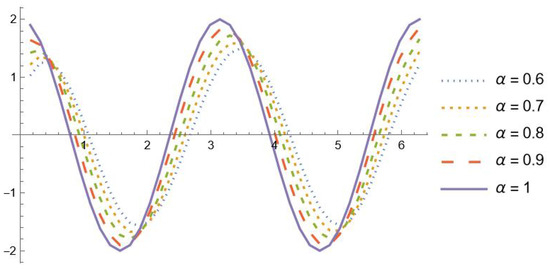
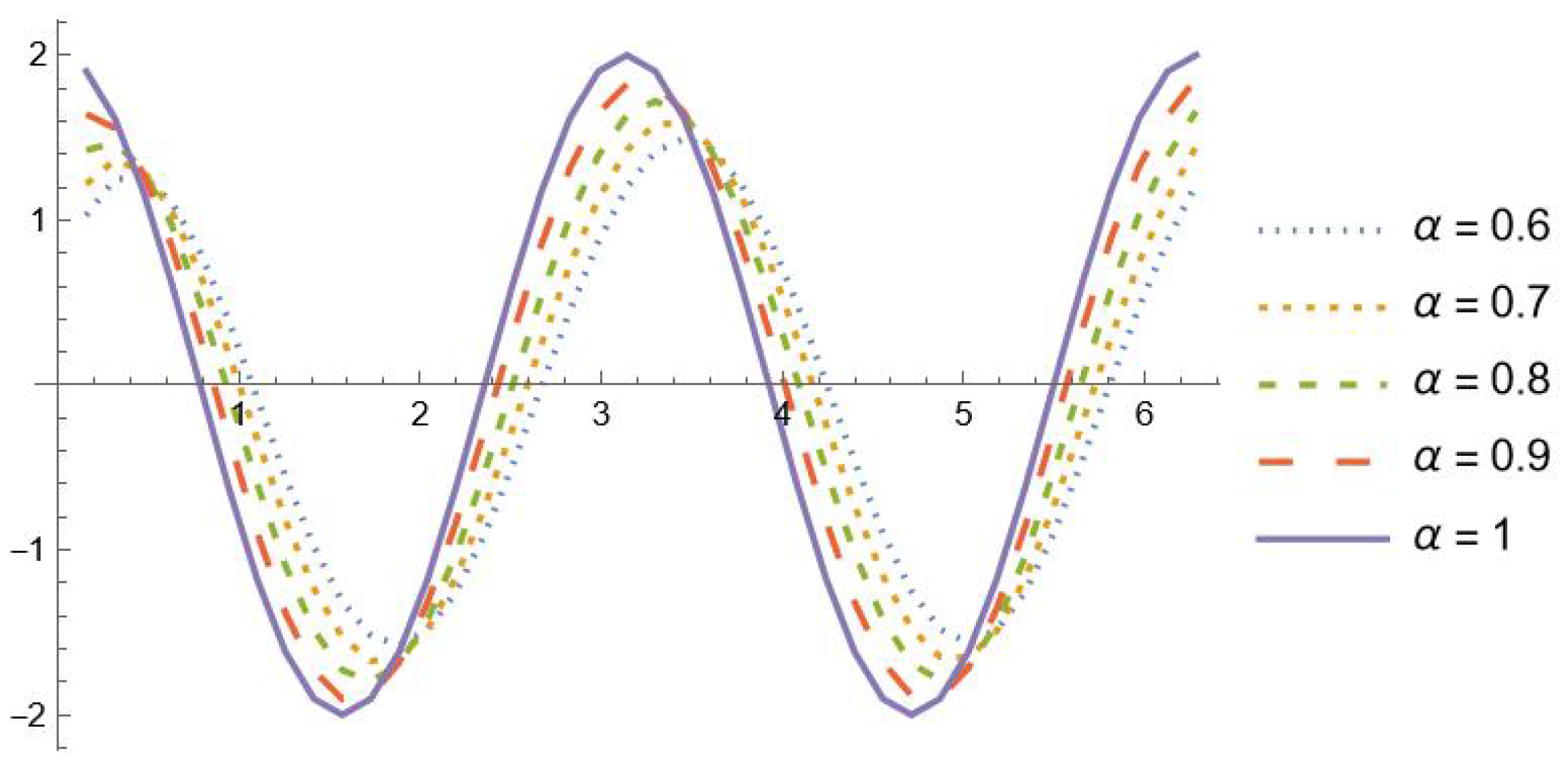
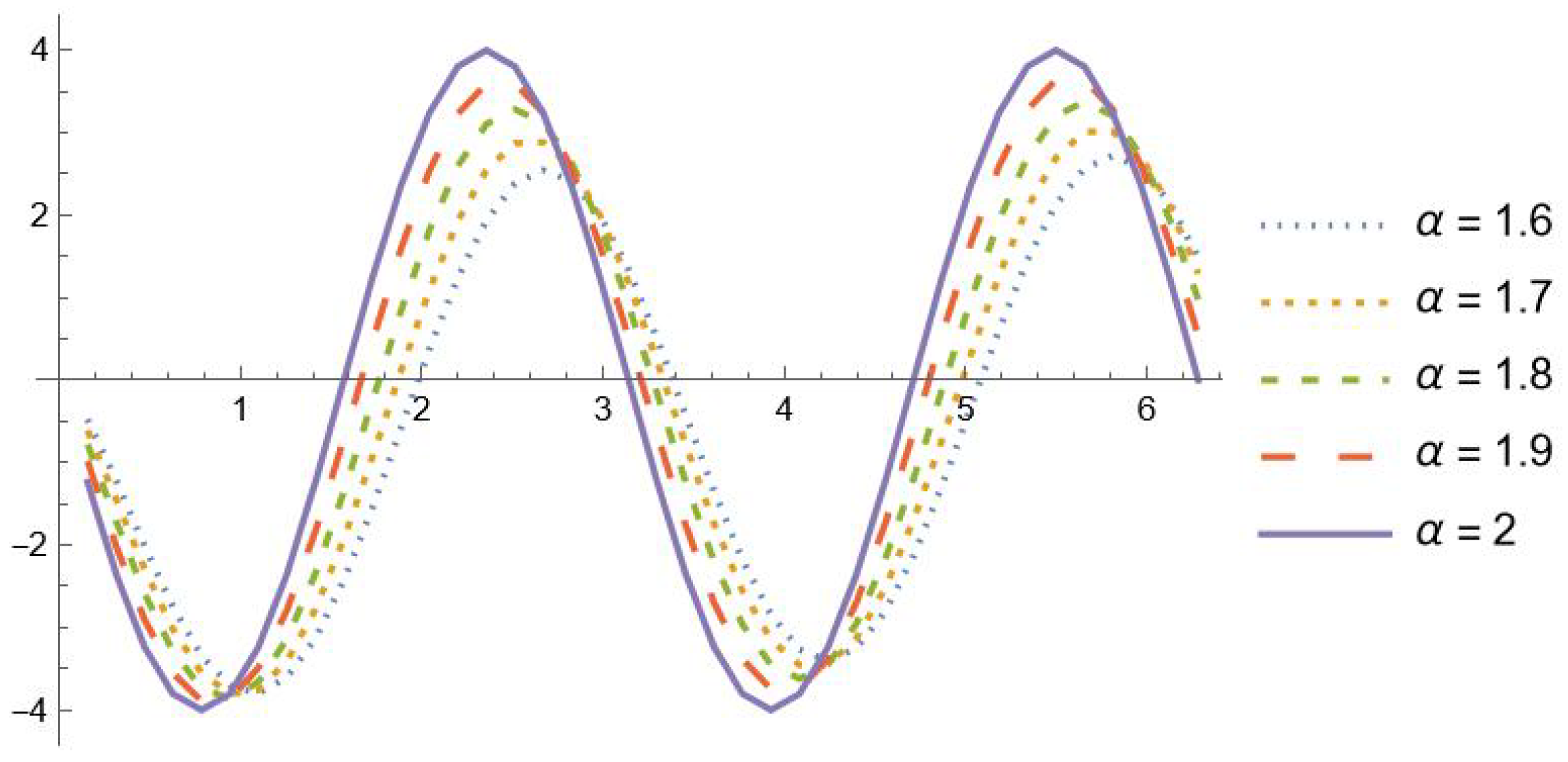
Moreover,

Table 2. $f\left(y\right)=sin\left(y\right),y\in [0,15]$.

n	$\mathit{e}\mathit{r}{\mathit{r}}_{\mathit{n}}^{\frac{1}{2}}$	$\mathit{e}\mathit{r}{\mathit{r}}_{\mathit{n}}^{\frac{3}{2}}$
10	4.418 $\times {10}^{-2}$	6.328 $\times {10}^{-2}$
15	3.430 $\times {10}^{-5}$	7.812 $\times {10}^{-5}$
20	2.412 $\times {10}^{-8}$	6.635 $\times {10}^{-8}$
25	9.930 $\times {10}^{-13}$	3.559 $\times {10}^{-12}$
30	8.428 $\times {10}^{-17}$	3.504 $\times {10}^{-16}$

reports the maximum absolute errors obtained when approximating $D^{\alpha }f,\alpha =\frac{1}{2},\frac{3}{2},$ in the interval $[0,15]$. Note that the precision is attained even in a wider range, though with a slightly greater number of interpolation nodes. In Figure 1 and Figure 2, the graphs of $\left(D_8^{\alpha }f\right)\left(x\right)$, $\alpha \in (0,1]$ and $\left(D_{10}^{\alpha }f\right)\left(x\right)$$\alpha \in (1,2]$ with $f\left(x\right)=sin\left(2\omega \right)$ are shown in the interval $[0,2\pi ]$. It is evident that the fractional derivatives $D^{\alpha }f$, $m-1<\alpha \le m$, tend to $D^{m}f$ for $\alpha \to m.$

Finally,

Table 3. $f\left(y\right)=sin\left(y\right)$.

n	$({\mathit{D}}_{\mathit{n}}^{\frac{1}{2}}\mathit{f})\left(1\right)$	${\mathit{err}}_{\mathit{n}}^{\frac{1}{2}}\left(1\right)$	$({\mathit{D}}_{\mathit{n}}^{\frac{3}{2}}\mathit{f})\left(1\right)$	${\mathit{err}}_{\mathit{n}}^{\frac{3}{2}}\left(1\right)$
5	0.8460567865921894	1.3196 $\times {10}^{-10}$	−0.6696801384860036	4.1210 $\times {10}^{-6}$
6	0.8460567867232841	8.6885 $\times {10}^{-13}$	−0.6696843635535760	1.0397 $\times {10}^{-7}$
7	0.8460567867241810	2.8051 $\times {10}^{-14}$	−0.6696842647065146	5.1288 $\times {10}^{-9}$
8	0.8460567867241531	1.9390 $\times {10}^{-16}$	−0.6696842594833962	9.4267 $\times {10}^{-11}$
9	0.8460567867241529	5.6655 $\times {10}^{-18}$	−0.6696842595738642	3.7993 $\times {10}^{-12}$
10	0.8460567867241529	1.9787 $\times {10}^{-20}$	−0.6696842595777186	5.4991 $\times {10}^{-14}$
11	0.8460567867241529	1.9094 $\times {10}^{-20}$	−0.6696842595776654	1.8776 $\times {10}^{-15}$
12	0.8460567867241529	1.8055 $\times {10}^{-20}$	−0.6696842595776635	2.2423 $\times {10}^{-17}$

reports the approximate values achieved by simultaneously approximating $D^{\alpha }f\left(1\right)$ for $\alpha =\frac{1}{2},\frac{3}{2}$. Here, the exact values computed using (23) are

$$(D^{\frac{1}{2}}f)\left(1\right)=0.8460567867241529(D^{\frac{3}{2}}f)\left(1\right)=-0.6696842595776635.$$

A comparison with the results in [24] (Tables 3.1 and 3.2) and [22] (Tables 11 and 12) shows that our procedure is more accurate and efficient.

Example 2. 

For $f\left(y\right)=y^{\theta }$, the analytical form of the Caputo fractional derivative is

$$\left(D^{\alpha }f\right)\left(y\right)=\frac{\Gamma (\theta +1)}{\Gamma (\theta +1-\alpha )}{y}^{\theta -\alpha }.$$

(24)

Table 4. $f\left(y\right)=y^{\frac{7}{2}},y\in [0,1]$.

n	$\mathit{e}\mathit{r}{\mathit{r}}_{\mathit{n}}^{\frac{1}{5}}$	$\mathit{e}\mathit{r}{\mathit{r}}_{\mathit{n}}^{\frac{1}{2}}$	$\mathit{e}\mathit{r}{\mathit{r}}_{\mathit{n}}^{\frac{4}{5}}$	$\mathit{e}\mathit{r}{\mathit{r}}_{\mathit{n}}^{\frac{6}{5}}$	$\mathit{e}\mathit{r}{\mathit{r}}_{\mathit{n}}^{\frac{3}{2}}$	$\mathit{e}\mathit{r}{\mathit{r}}_{\mathit{n}}^{\frac{9}{5}}$
10	7.125 $\times {10}^{-7}$	1.719 $\times {10}^{-6}$	5.035 $\times {10}^{-6}$	3.068 $\times {10}^{-5}$	6.414 $\times {10}^{-5}$	1.923 $\times {10}^{-4}$
20	8.536 $\times {10}^{-9}$	3.078 $\times {10}^{-8}$	8.866 $\times {10}^{-8}$	7.494 $\times {10}^{-7}$	2.419 $\times {10}^{-6}$	7.936 $\times {10}^{-6}$
40	8.919 $\times {10}^{-11}$	4.852 $\times {10}^{-10}$	2.101 $\times {10}^{-9}$	2.300 $\times {10}^{-8}$	7.197 $\times {10}^{-8}$	2.439 $\times {10}^{-7}$
80	5.629 $\times {10}^{-13}$	4.005 $\times {10}^{-12}$	3.280 $\times {10}^{-11}$	6.404 $\times {10}^{-10}$	1.703 $\times {10}^{-9}$	4.651 $\times {10}^{-9}$

shows the approximations of $D^{\alpha }f$ with $\theta =\frac{7}{2}$ in the interval $[0,1]$ for different choices of α. The obtained results are again better than those in [13] (second row of Table 1), in particular for larger values of α.

4. Application to the Bagley–Torvik IVP

In this section, we show how the procedure introduced in the previous section can be used to construct a Nyström-type method for solving the Volterra integral equation equivalent to the Bagley–Torvik IVP.

In [7,8], Bagley and Torvik studied the motion of a rigid plate immersed in an infinite Newtonian fluid. They proved that the displacement u of the plate at time t is described by the equation

$$u^{″}\left(y\right)+\lambda \left(D^{\frac{3}{2}}u\right)\left(y\right)+\sigma u\left(y\right)=\mu h\left(y\right),y\in [0,T],$$

where $D^{\frac{3}{2}}u$ is the Caputo fractional derivative of order $\frac{3}{2}$, h is the force applied to the plate, and T is the fixed maximum observation time. The quantities $\lambda ,\sigma ,\mu$ are connected with the mass $\mathrm{M}$ and area S of the plate as well as with the stiffness constant K, fluidity $\rho$, and fluid viscosity $\nu$ by the following relations:

$$\lambda =\frac{2S\sqrt{\nu \rho }}{\mathrm{M}},\sigma =\frac{K}{\mathrm{M}},\mu =\frac{1}{\mathrm{M}}.$$

Assuming that we know the initial displacement and velocity at the initial time $t=0$, the following Bagley–Torvik IVP is deduced:

$$\left\{\begin{array}{c}{u}^{″}\left(y\right)+\lambda (D^{\frac{3}{2}}u)\left(y\right)+\sigma u\left(y\right)=\mu h\left(y\right),y\in [0,T],\hfill \\ u\left(0\right)={\gamma }_1,u^{\prime }\left(0\right)={\gamma }_2.\hfill \end{array}\right.$$

(25)

The following theorem stating the existence and uniqueness of the solution of Problem (25) in the space $C^2\left([0,T]\right)$ was proved in [39].

Theorem 3. 

If $h\in C^0\left([0,T]\right)$ then the Bagley–Torvik IVP admits a unique solution $u\in C^2\left([0,T]\right).$

As previously stated, our numerical method consists in approximating the solutions of a second kind Volterra integral equation (VIE) that is equivalent to the IVP problem (25). The next lemma introduces the VIE and establishes the equivalence between its solutions and the solutions of (25) in the space $A{C}^1\left([0,T]\right)$, where $u\in A{C}^1\left([0,T]\right)$ if and only if $u^{″}\left(t\right)$ exists for a.e. $t\in [0,T]$ with $u^{″}\in L^1\left([0,T]\right)$ and such that

$$u^{\prime }\left(t\right)-u^{\prime }\left(0\right)={\int }_0^t{u}^{″}\left(s\right)ds,\forall t\in [0,T].$$

Lemma 1. 

Let $h\in L^1\left([0,T]\right)$; then, $u\in A{C}^1\left([0,T]\right)$ is a solution of (25) if and only if it is a solution of the second kind VIE:

$$u\left(x\right)+\lambda {\int }_0^x(x-y)\left(D^{\frac{3}{u}}\right)\left(y\right)dy+\sigma {\int }_0^x(x-y)u\left(y\right)dy=\mu {\int }_0^x(x-y)h\left(y\right)dy+{\gamma }_{2}x+{\gamma }_1,$$

(26)

for $x\in [0,T].$

Remark 6. 

If $h\in C^0\left([0,T]\right)$, then the equivalence stated in Lemma 1 holds true in the space $C^2\left([0,T]\right)$.

With the change of variable $t=x/T,$ the integral Equation (26) becomes

$$f\left(t\right)+\overline{\lambda }{\int }_0^t(t-y)(D^{\frac{3}{2}}f)\left(y\right)dy+\overline{\sigma }{\int }_0^t(t-y)f\left(y\right)dy=\overline{\mu }{\int }_0^t(t-y)h\left(yT\right)dy+{\gamma }_{2}tT+{\gamma }_1,$$

(27)

where $t\in [0,1]$, $\overline{\lambda }=\sqrt{T}\lambda$, $\overline{\sigma }=T^2\sigma$, and $\overline{\mu }=T^2\mu$. After determining f in (27), u in (26) (or, equivalently, the solution of the Bagley–Torvik IVP (25)) can be computed through

$$u\left(x\right)=f\left(\frac{x}{T}\right),x\in [0,T].$$

(28)

Letting

$$\left(Kf\right)\left(t\right)={\int }_0^t(t-y)(D^{\frac{3}{2}}f)\left(y\right)dy,$$

$$\left(Hf\right)\left(t\right)={\int }_0^t(t-y)f\left(y\right)dy,$$

$$g\left(t\right)=\overline{\mu }{\int }_0^t(t-y)h\left(yT\right)dy+{\gamma }_{2}tT+{\gamma }_1,$$

and denoting the identity operator by I, Equation (27) can be written as

$$(I+\overline{\lambda }K+\overline{\sigma }H)f\left(t\right)=g\left(t\right)t\in [0,1].$$

(29)

Supported by Theorem 3 and Remark 6, we study the above equation in the space $C^2$, proving the following theorem about its unisolvence.

Theorem 4. 

If $\mathrm{Ker}(I+\overline{\lambda }K+\overline{\sigma }H)=\left\{0\right\}$ in $C^2$, then Equation (29) admits a unique solution $f\in C^2$ for any $g\in C^2$. Moreover, if $g\in C^{2+\frac{1}{2}}$, then f belongs to $C^{2+\frac{1}{2}}$ as well.

Remark 7. 

Under the assumption that $h\in C^{0+\frac{1}{2}}$, the function $g\in C^{2+\frac{1}{2}}$, as $g^{″}\left(t\right)=\overline{\mu }h\left(tT\right).$

Now, we propose a Nyström-type method based on the approximation of $\left(Kf\right)\left(t\right)$ by

$$\left(K_{n}f\right)\left(t\right)={\int }_0^t(t-y)(D_n^{\frac{3}{2}}f)\left(y\right)dy,$$

(30)

where $D_n^{\frac{3}{2}}f$ is defined in (18) with $\gamma =\delta =-\frac{1}{2}$. In addition, we approximate $\left(Hf\right)\left(t\right)$ by

$$\left(H_{n}f\right)\left(t\right)={\int }_0^t(t-y)L_{n,1,1}(f,y)dy,$$

(31)

where we lighten the notation by denoting the interpolating polynomial based on the zeros of $x(x-1)p_n(v^{-\frac{1}{2},-\frac{1}{2}},x)$ simply by $L_{n,1,1}(f,x)$.

Hence, we obtain the following finite dimensional equation:

$$(I+\overline{\lambda }{K}_n+\overline{\sigma }{H}_n)f_n\left(t\right)=g\left(t\right),t\in [0,1].$$

(32)

In view of (9) and (19), we have

$$\begin{array}{ccc}\hfill \left(K_{n}f\right)\left(t\right)& =& {\int }_0^t(t-y)(D_n^{\frac{3}{2}}f)\left(y\right)dy=t^2{\int }_0^1(1-z)(D_n^{\frac{3}{2}}f)\left(zt\right)dz\hfill \\ & =& \frac{t^{\frac{5}{2}}}{\sqrt{\pi }}\sum _{k=1}^{n+2}f\left(t_k\right){\int }_0^1{\int }_0^1{\ell }_k^{″}\left(szt\right)v^{-\frac{1}{2},0}\left(s\right)v^{1,\frac{1}{2}}\left(z\right)dsdz\hfill \\ & =:& \frac{t^{\frac{5}{2}}}{\sqrt{\pi }}\sum _{k=1}^{n+2}f\left(t_k\right)c_k\left(t\right).\hfill \end{array}$$

The integrals $c_k\left(t\right),k=1,\dots ,n+2$ can be exactly computed by the Gauss–Jacobi cubature rule of order N with respect to the bivariate weight function $v^{m-\alpha -1,0}\left(t\right)v^{1,m-\alpha }\left(z\right)$, i.e.,

$$c_k\left(t\right)=\sum _{i=1}^N\sum _{j=1}^N{\ell }_k^{″}\left(x_i^{-\frac{1}{2},0}{x}_j^{1,\frac{1}{2}}t\right){\lambda }_{N,i}^{-\frac{1}{2},0}{\lambda }_{N,j}^{1,\frac{1}{2}},N=⌈\frac{n}{2}⌉.$$

We point out that the cubature formula is exact for any polynomial of degree $2N-1$ separately in each variable $t,z$ (see, e.g., [40]). Moreover, from (9) we obtain

$$\begin{array}{ccc}\hfill \left(H_{n}f\right)\left(t\right)& =& {\int }_0^t(t-y)L_{n,1,1}(f,y)dy=\sum _{k=1}^{n+2}f\left(t_k\right){\int }_0^t(t-y){\ell }_k\left(y\right)dy\hfill \\ & =& t^2\sum _{k=1}^{n+2}f\left(t_k\right){\int }_0^1{\ell }_k\left(zt\right)v^{1,0}\left(z\right)dz=:t^2\sum _{k=1}^{n+2}f\left(t_k\right){\overline{c}}_k\left(t\right),\hfill \end{array}$$

where the integrals ${\overline{c}}_k\left(t\right),k=1,\dots ,n+2$ can be exactly computed by the N-Gauss–Jacobi rule with $N=\lceil \frac{n+1}{2}\rceil ,$ with respect to the weight function $v^{1,0}\left(z\right)=(1-z)$, obtaining

$${\overline{c}}_k\left(t\right)=\sum _{i=1}^N{\ell }_k\left(x_i^{1,0}t\right){\lambda }_{N,i}^{1,0}.$$

Hence, taking into account the initial condition $f\left(0\right)=f\left(t_1\right)={\gamma }_1$, we obtain

$$\overline{\lambda }\left(K_{n}f\right)\left(t\right)=\frac{\overline{\lambda }}{\sqrt{\pi }}{t}^{\frac{5}{2}}\sum _{k=1}^{n+2}f\left(t_k\right)c_k\left(t\right)=\frac{\overline{\lambda }}{\sqrt{\pi }}{t}^{\frac{5}{2}}\left[{\gamma }_1{c}_1\left(t\right)+\sum _{k=2}^{n+2}f\left(t_k\right)c_k\left(t\right)\right]$$

and

$$\overline{\sigma }\left(H_{n}f\right)\left(t\right)=\overline{\sigma }{t}^2\sum _{k=1}^{n+2}f\left(x_k\right){\overline{c}}_k\left(t\right)=\overline{\sigma }{t}^2\left[{\gamma }_1{\overline{c}}_1\left(t\right)+\sum _{k=2}^{n+2}f\left(t_k\right){\overline{c}}_k\left(t\right)\right].$$

As a consequence, Equation (32) becomes

$$f_n\left(t\right)+\sum _{k=2}^{n+2}\left[\frac{\overline{\lambda }}{\sqrt{\pi }}{t}^{\frac{5}{2}}{c}_k\left(t\right)+\overline{\sigma }{t}^2{\overline{c}}_k\left(t\right)\right]f_n\left(t_k\right)=g\left(t\right)-{\gamma }_1\left[\frac{\overline{\lambda }}{\sqrt{\pi }}{t}^{\frac{5}{2}}{c}_1\left(t\right)+\overline{\sigma }{t}^2{\overline{c}}_1\left(t\right)\right],$$

and by collocation at $t_2,\dots ,t_{n+2}$ we obtain the equivalent linear system of order $n+1$:

$$\begin{array}{c}\hfill \sum _{k=2}^{n+2}\left[{\delta }_{j,k}+\frac{\overline{\lambda }}{\sqrt{\pi }}{t}_j^{\frac{5}{2}}{c}_k\left(t_j\right)+\overline{\sigma }{t}_j^2{\overline{c}}_k\left(t_j\right)\right]a_k=g\left(t_j\right)-{\gamma }_1\left[\frac{\overline{\lambda }}{\sqrt{\pi }}{t}_j^{\frac{5}{2}}{c}_1\left(t_j\right)+\overline{\sigma }{t}_j^2{\overline{c}}_1\left(t_j\right)\right],\\ \hfill j=2,\dots ,n+2,\end{array}$$

(33)

in the unknowns ${\{a_k:=f_n\left(t_k\right)\}}_{k=2}^{n+2}.$

If ${(a_2^{*},\dots ,a_{n+2}^{*})}^T$ is a solution of the linear system in (33), then, letting $a_1^{*}={\gamma }_1$, the Nyström interpolant

$$f_n\left(t\right)=g\left(t\right)-\sum _{k=1}^{n+2}\left[\frac{\overline{\lambda }}{\sqrt{\pi }}{t}^{\frac{5}{2}}{c}_k\left(t\right)+\overline{\sigma }{t}^2{\overline{c}}_k\left(t\right)\right]a_k^{*}$$

(34)

is a solution of the discrete Equation (32) and vice versa.

In the next theorem, we provide sufficient conditions assuring the convergence of the proposed method along with estimates of the error depending on the smoothness of the unknown solution.

Theorem 5. 

Assuming that $\mathrm{Ker}(I+\overline{\lambda }K+\overline{\sigma }H)=\left\{0\right\}$ in $C^2$, the inverses of the operators $I+\overline{\lambda }{K}_n+\overline{\sigma }{H}_n:C^2\to C^2$ exist and are uniformly bounded and $g\in C^{2+\frac{1}{2}}$. Then, for sufficiently large n (say, $n\ge n_0$), the Nyström interpolating functions $f_n$ converge to the exact solution f of the VIE (29) and

$$\parallel f-f_n{\parallel }_{\infty }=\mathcal{O}\left(\frac{logn}{\sqrt{n}}\right).$$

(35)

Moreover, if $f\in C^{q+\frac{1}{2}},$$q>2$, then

$$\parallel f-f_n{\parallel }_{\infty }=\mathcal{O}\left(\frac{logn}{n^{q-\frac{3}{2}}}\right).$$

(36)

Here, the constants in “$\mathcal{O}$” are independent of n.

Coming back to the Bagley–Torvik IVP from Theorem 5 and Remark 7, it is easy to deduce the following result.

Corollary 1. 

Under the assumptions of the previous theorem, if $h\in C^{0+\frac{1}{2}}\left([0,T]\right)$ for all sufficiently large n (say, $n\ge n_0$), then the sequence ${\left\{u_n\right\}}_n$, with $u_n\left(t\right)=f_n\left(\frac{t}{T}\right),t\in [0,T]$ converges to the exact solution u of the Bagley–Torvik IVP and

$$\parallel u-u_n{\parallel }_{\infty }=\mathcal{O}\left(\frac{logn}{\sqrt{n}}\right).$$

Numerical Tests on the Bagley–Torvik IVP

We now propose some numerical tests confirming the effectiveness of the method described in Section 4 and the approximation proposed in Section 3 for Caputo fractional derivatives. In the following examples,

$$Er{r}_n\left(\overline{y}\right)=|u\left(\overline{y}\right)-u_n\left(\overline{y}\right)|,$$

is the maximum absolute error computed over a sufficiently large set ${\xi }_i,i=1,\dots ,\mu ,$ of $\mu$ equispaced points in $[0,T],$ i.e.,

$${\overline{Err}}_n=\underset{i=1,\dots ,\mu }{max}Er{r}_n\left({\xi }_i\right).$$

In Example 5, we make a comparison with the method proposed in [13].

Example 3. 

Consider the following Bagley–Torvik IVP:

$$\left\{\begin{array}{c}{u}^{″}\left(t\right)+\frac{1}{100}(D^{\frac{3}{2}}u)\left(t\right)+\frac{1}{200}u\left(t\right)=h\left(t\right),0\le t\le T,\hfill \\ \\ u\left(0\right)=0,u^{\prime }\left(0\right)=0.\hfill \end{array}\right.$$

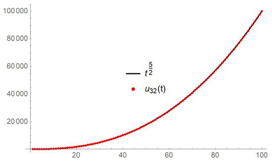
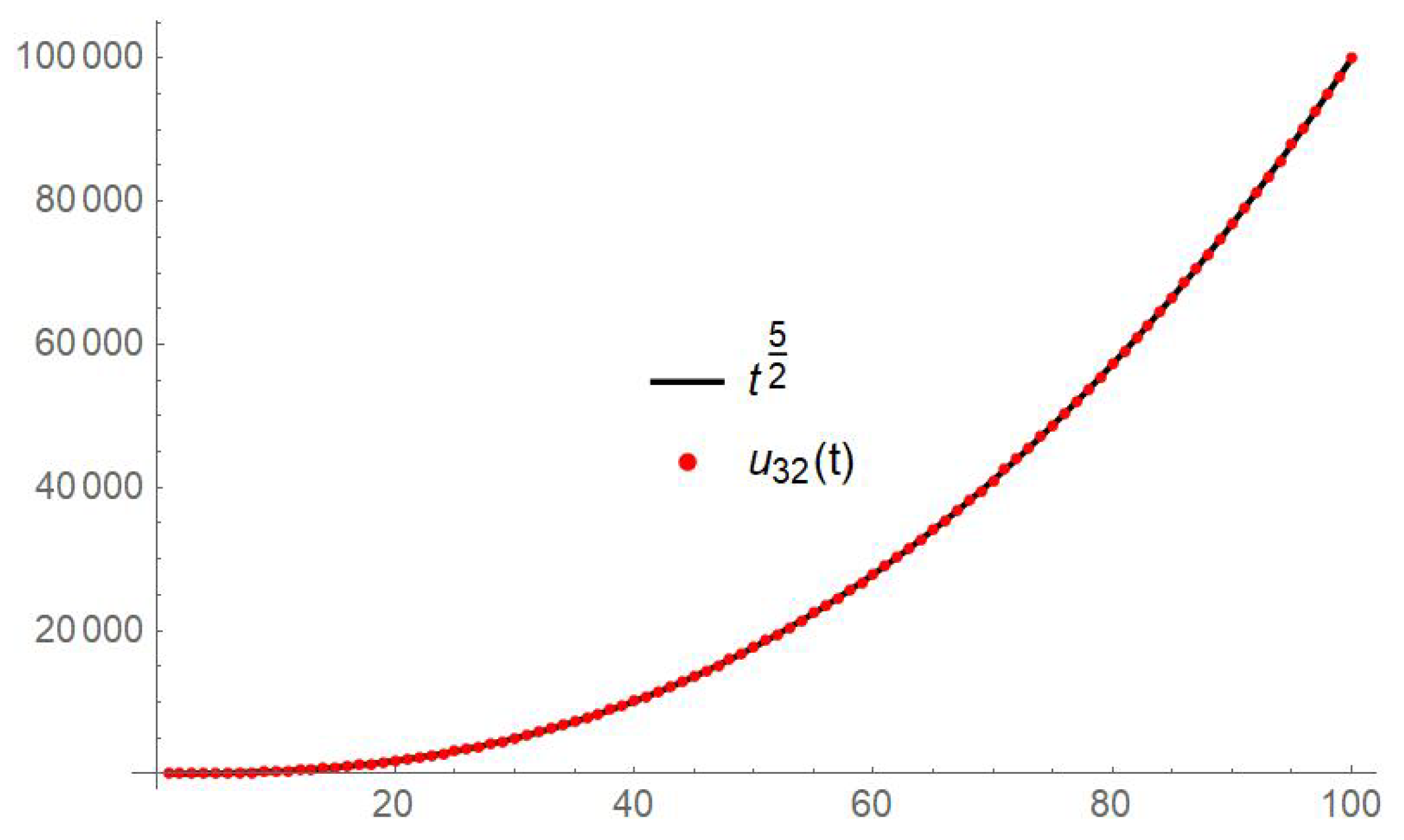
If we choose $h\left(t\right)=\frac{t^{\frac{5}{2}}}{200}+\frac{3\sqrt{\pi }t}{160}+\frac{15\sqrt{t}}{4}\in C^{0+\frac{1}{2}}\left([0,T]\right)$, then the exact solution is $u\left(t\right)=t^{\frac{5}{2}}\in C^{2+\frac{1}{2}}\left([0,T]\right)$.

Table 5. Example 3.

n	${\mathit{Err}}_{\mathit{n}}\left(1\right)$	${\mathit{Err}}_{\mathit{n}}\left(2.5\right)$	${\mathit{Err}}_{\mathit{n}}\left(4.5\right)$
4	5.27 $\times {10}^{-4}$	1.53 $\times {10}^{-3}$	3.73 $\times {10}^{-3}$
8	4.57 $\times {10}^{-5}$	1.93 $\times {10}^{-4}$	4.67 $\times {10}^{-4}$
16	6.26 $\times {10}^{-6}$	2.45 $\times {10}^{-5}$	5.88 $\times {10}^{-5}$
32	7.88 $\times {10}^{-7}$	3.08 $\times {10}^{-6}$	7.36 $\times {10}^{-6}$
64	9.82 $\times {10}^{-8}$	3.85 $\times {10}^{-7}$	9.20 $\times {10}^{-7}$

reports the values of the approximant $u_n\left(t\right)$ for $t=1,2.5,4.5$. As can be seen, according to our theoretical expectations it is necessary to increase n in order to attain exact decimal digits. Figure 3 compares the graphs of the exact solution $u\left(t\right)$ and its approximation $u_{32}\left(t\right)$ in the interval $[0,100].$

Example 4. 

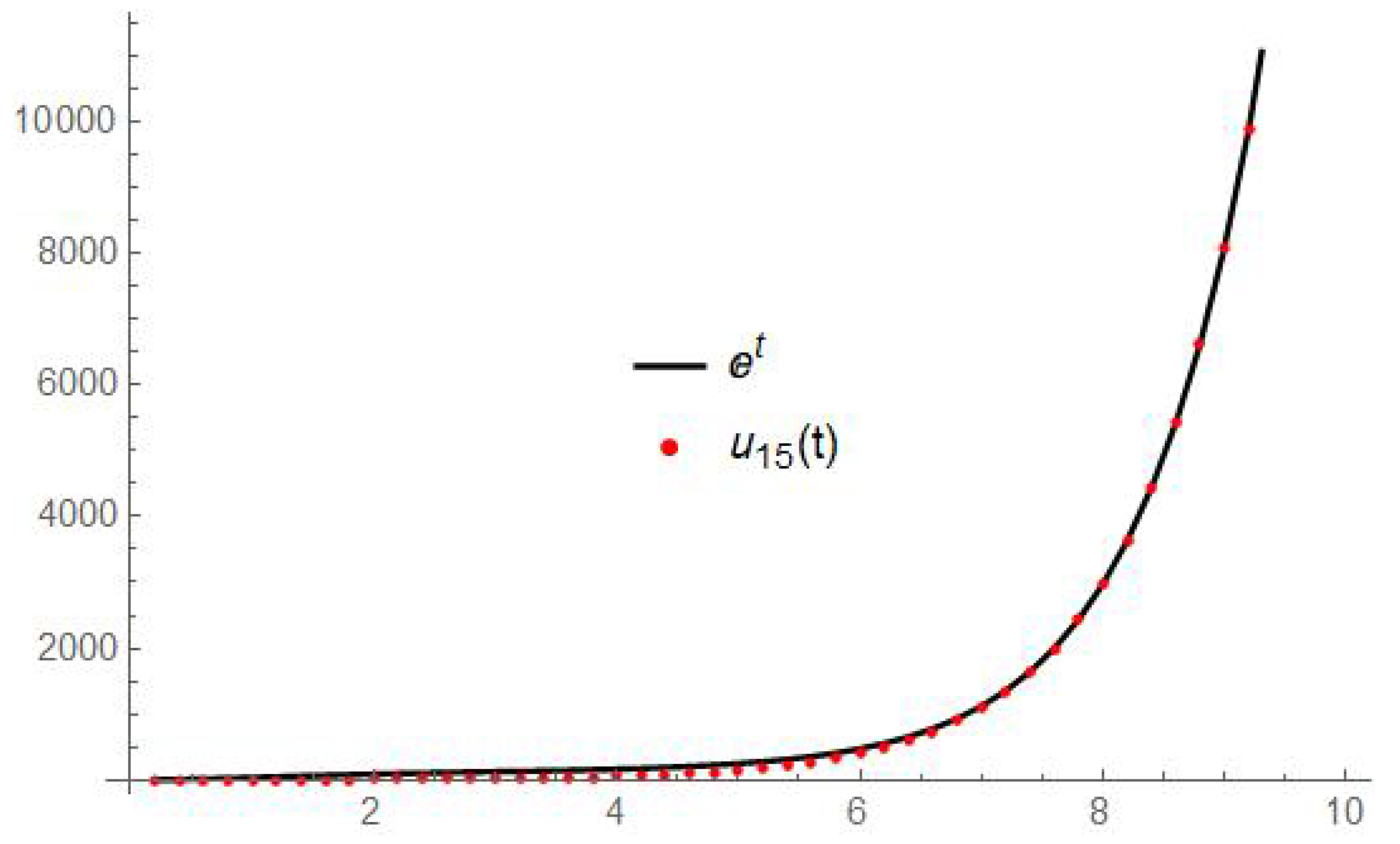
Let us consider

$$\left\{\begin{array}{c}{u}^{″}\left(t\right)+\frac{1}{2}(D^{\frac{3}{2}}u)\left(t\right)+\frac{1}{2}u\left(t\right)=h\left(t\right),0\le t\le T,\hfill \\ \\ u\left(0\right)=1,u^{\prime }\left(0\right)=2,\hfill \end{array}\right.$$

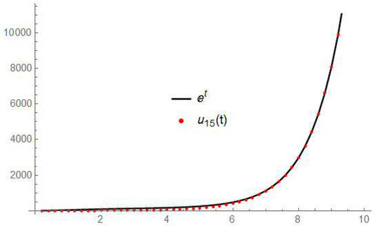
with $h\left(t\right)=\frac{3}{2}{e}^t+\frac{e^t}{2\sqrt{\pi }}\gamma \left(\frac{1}{2},t\right)$, where $\gamma (a,z)$ is the incomplete Gamma function. The exact solution is $u\left(t\right)=e^t$. In this case, we expect very fast convergence, with $u\left(t\right)$ being very smooth. This is confirmed by the numerical results presented in

Table 6. Example 4.

n	${\mathit{Err}}_{\mathit{n}}\left(0.25\right)$	${\mathit{Err}}_{\mathit{n}}\left(1.5\right)$	${\mathit{Err}}_{\mathit{n}}\left(2.5\right)$
5	7.82 $\times {10}^{-5}$	2.72 $\times {10}^{-4}$	7.98 $\times {10}^{-4}$
10	5.66 $\times {10}^{-11}$	1.53 $\times {10}^{-9}$	2.19 $\times {10}^{-9}$
15	1.91 $\times {10}^{-15}$	2.69 $\times {10}^{-14}$	4.71 $\times {10}^{-14}$
17	4.68 $\times {10}^{-16}$	1.24 $\times {10}^{-15}$	4.70 $\times {10}^{-15}$

. The graphs of the exact solution and its approximation $u_{15}$ are shown in Figure 4.

Example 5. 

We take the following IVP:

$$\left\{\begin{array}{c}{u}^{″}\left(t\right)+(D^{\frac{3}{2}}u)\left(t\right)+u\left(t\right)=eh\left(t\right),0\le t\le 1,\hfill \\ \\ u\left(0\right)=0,u^{\prime }\left(0\right)=\omega \hfill \end{array}\right.$$

with $h\left(t\right)$ such that $u\left(t\right)=sin\left(\omega t\right)$. Again, in this case the solution is very smooth, and, as shown in

Table 7. Example 5.

n	${\overline{\mathit{Err}}}_{\mathit{n}}(\mathit{\omega }=1)$	${\overline{\mathit{Err}}}_{\mathit{n}}(\mathit{\omega }=2\mathit{\pi })$	${\overline{\mathit{Err}}}_{\mathit{n}}(\mathit{\omega }=4\mathit{\pi })$
4	1.720 $\times {10}^{-6}$	8.151 $\times {10}^{-2}$	2.258 e + 0
8	1.366 $\times {10}^{-12}$	7.173 $\times {10}^{-5}$	6.502 $\times {10}^{-2}$
16	3.657 $\times {10}^{-16}$	7.028 $\times {10}^{-13}$	3.247 $\times {10}^{-7}$
23	3.490 $\times {10}^{-16}$	2.327 $\times {10}^{-16}$	9.376 $\times {10}^{-13}$
27	4.587 $\times {10}^{-16}$	5.254 $\times {10}^{-16}$	1.590 $\times {10}^{-16}$

, the convergence is very fast.

This example was also considered in [13] (Example 6.3). We point out that they used a procedure quite different from the one that we propose in Section 4: they numerically solved the IVP (25) directly without considering the equivalent VIE (26). Comparing the results in [13] (Table 7) with those in Table 7, it can be observed that our Nyström method is faster for any choice of ω.

5. Proofs

Proof of Theorem 2. 

Using (7), we deduce

$$\begin{array}{ccc}\hfill |\left(D^{\alpha }f\right)\left(y\right)-\left(D_n^{\alpha }f\right)\left(y\right)|& \le & \frac{1}{\sqrt{\pi }}{\int }_0^y{(y-x)}^{m-\alpha -1}|f^{\left(m\right)}\left(x\right)-L_{n,r,s}^{\left(m\right)}(v^{\gamma ,\delta },f,x)|dx\hfill \\ & \le & \frac{1}{\sqrt{\pi }}{\parallel f^{\left(m\right)}-L_{n,r,s}^{\left(m\right)}(v^{\gamma ,\delta },f)\parallel }_{\infty }{\int }_0^y{(y-x)}^{m-\alpha -1}dx\hfill \\ & \le & \mathcal{C}\frac{E_{n-q}\left(f^{\left(q\right)}\right)}{n^{q-h}}logn,\hfill \end{array}$$

i.e., (21) for $q\ge m.$ If $f\in C^{q+\mu }$, then (22) follows per (3). □

Proof of Lemma 1. 

Let $u\in A{C}^1\left([0,T]\right)$ be a solution of (25). Letting $\phi \left(y\right)=-\lambda (D^{\frac{3}{2}}u)\left(y\right)-\sigma u\left(y\right)+\mu h\left(y\right)$, (25) becomes

$$\left\{\begin{array}{c}{u}^{″}\left(y\right)=\phi \left(y\right),\hfill \\ u\left(0\right)={\gamma }_1,u^{\prime }\left(0\right)={\gamma }_2.\hfill \end{array}\right.$$

We first recall that, by definition, $D^{\frac{3}{2}}u\in L^1\left([0,T]\right)$ for $u\in A{C}^1\left([0,T]\right)$ (see [36] (Definition 2.4)). Then, under the assumption $h\in L^1\left([0,T]\right)$, we deduce $\phi \left(y\right)\in L^1$; using the fundamental theorem of calculus together with the initial conditions, we obtain

$$u^{\prime }\left(t\right)={\int }_0^t\phi \left(y\right)dy+{\gamma }_2$$

and

$$u\left(s\right)={\int }_0^s{u}^{\prime }\left(t\right)dt+{\gamma }_1={\int }_0^s\left[{\int }_0^t\phi \left(y\right)dy+{\gamma }_2\right]dt+{\gamma }_1.$$

As it is well-known that [41]

$${\int }_0^s{\int }_0^t\phi \left(y\right)dydt={\int }_0^s(s-y)\phi \left(y\right)dy,$$

we deduce

$$u\left(s\right)={\int }_0^s(s-y)\phi \left(y\right)dy+{\gamma }_{2}s+{\gamma }_1,$$

(37)

i.e., (26), recalling the expression of $\phi \left(y\right)$. Thus, u is also a solution of (26).

Now, if $u\in A{C}^1\left([0,T]\right)$ is a solution of (26), by differentiating both sides of Equation (26) in the form of (37) twice we obtain

$$u^{″}\left(y\right)=\phi \left(y\right)=-\lambda (D^{\frac{3}{2}}u)\left(y\right)-\sigma u\left(y\right)+\mu h\left(y\right).$$

Moreover, from (37) it is easily seen that

$$u\left(0\right)={\gamma }_1\mathrm{and}{u}^{\prime }\left(0\right)={\gamma }_2.$$

Then, u is also a solution of (25). □

Proof of Theorem 4. 

If we prove that the operators $H,K:C^0\to C^2$ are compact, then under the assumption $\mathrm{Ker}(I+\overline{\lambda }K+\overline{\sigma }H)=\left\{0\right\}$ in $C^2$ the unisolvence in $C^2$ of (29) for any $g\in C^2$ follows by Fredholm’s alternative theorem.

We first prove that the operator $H:C^0\to C^2$ is continuous. We have

$$\left|\left(Hf\right)\left(t\right)\right|\le {\parallel f\parallel }_{\infty }{\int }_0^t(t-y)dy\le \mathcal{C}{\parallel f\parallel }_{\infty }.$$

Moreover, taking into account that

$${\left(Hf\right)}^{″}\left(t\right)=f\left(t\right),$$

(38)

it is easily seen that

$${\parallel \left(Hf\right)}^{″}{\parallel }_{\infty }={\parallel f\parallel }_{\infty }.$$

Then,

$${\parallel Hf\parallel }_{2,\infty }\le \mathcal{C}{\parallel f\parallel }_{\infty },$$

i.e., $H:C^0\to C^2$ is continuous. Now, because $C^2$ is compactly embedded in $C^0$ (for example, see [42] (Lemma 3.2)), from the continuity of the operator $H:C^0\to C^2$ we deduce the compactness of the operator $H:C^2\to C^2$.

To prove the compactness of the operator $K:C^2\to C^2$, we first note that it can be written as the composition of the following operators: $D^2:C^2\to C^0$, $J^{\frac{1}{2}}:C^0\to C^0$ and $H:C^0\to C^2$, i.e.,

$$Kf=H{D}^{\frac{3}{2}}f=H{J}^{\frac{1}{2}}{D}^{2}f.$$

(39)

From the continuity of $D^2:C^2\to C^0$ and $H:C^0\to C^2$ and the compactness of $J^{\frac{1}{2}}:C^0\to C^0$, we deduce the compactness of $K:C^2\to C^2$.

Using (38), (39), and (17), it is easy to deduce that if $f\in C^2$, then $Kf,Hf\in C^{2+\frac{1}{2}}$; thus, if $g\in C^{2+\frac{1}{2}}$, then $f=g-\overline{\lambda }K-\overline{\sigma }H$ belongs to $C^{2+\frac{1}{2}}$. □

Proof of Theorem 5. 

In order to prove (35), we first note that

$$(f-f_n)={(I+\overline{\lambda }{K}_n+\overline{\sigma }{H}_n)}^{-1}[(K-K_n)f-(H-H_n)f].$$

Under our assumptions

$$\underset{n\ge n_0}{sup}{\parallel {(I+\overline{\lambda }{K}_n+\overline{\sigma }{H}_n)}^{-1}\parallel }_{C^2\to C^2}\le \mathcal{C},\mathcal{C}\ne \mathcal{C}\left(n\right),$$

we obtain

$$\parallel f-f_n{\parallel }_2\le \mathcal{C}\left[\parallel (K-K_n){f\parallel }_2+{\parallel (H-H_n)f\parallel }_2\right].$$

Now, taking into account (39) and that $H_{n}f=H{L}_{n,1,1}\left(f\right)$ and $K_{n}f=H{D}_n^{\frac{3}{2}}f$, by using (38) it is easy to verify that

$$\parallel (K-K_n){f\parallel }_{2,\infty }\le \mathcal{C}{\parallel D^{\frac{3}{2}}f-D_n^{\frac{3}{2}}f\parallel }_{\infty }$$

and

$$\parallel (H-H_n){f\parallel }_{2,\infty }\le \mathcal{C}{\parallel f-L_{n,1,1}\left(f\right)\parallel }_{\infty }.$$

Then, using (22) and (7), (35) and (36) follow. □

6. Conclusions

In this work, we have developed a global method for numerically evaluating fractional derivatives of f of order $\alpha$. The interpolating process is essentially based on Jacobi zeros, and makes use of the additional nodes method [1] to approximate the m-th derivative of f by the m-th derivative of the interpolating polynomial. Error estimates are provided in spaces of q times differentiable functions with $q>m$, and some numerical tests are presented to confirm the theoretical estimates. As an application, the proposed method is implemented to approximate the solution of the VIE equivalent to the Bagley–Torvik IVP. We also present a detailed error analysis for the Nyström-type method proposed for the VIE. The efficiency of our numerical approach for approximating fractional derivatives is tested both directly through numerical tests and indirectly through implementation of the Nyström method, with the numerical experimentation confirming the theoretical results. From the implementation point of view, we show how to take advantage of simultaneous approximation; in approximating more than one $D^{\alpha }f$, it is sometimes the case that the required number of function evaluations is the same, while at other times it may be slightly more depending on the number of additional nodes. Finally, the dependence of the errors on the best polynomial approximation assures fast theoretical convergence, allowing finer results to be obtained with a lower number of interpolation nodes.

References

- Mastroianni, G. Uniform convergence of derivatives of Lagrange interpolation. J. Comput. Appl. Math. 1992, 43, 37–51. [Google Scholar] [CrossRef]
- Morgado, M.L.; Lima, P.M.; Mendes, M. Numerical Solution of the Time Fractional Cable Equation. In Springer Proceedings in Mathematics and Statistics, Proceedings of the ICDDEA 2019, Lisbon, Portugal, 1–5 July 2019; Springer: Cham, Switzerland, 2020; Volume 333, pp. 603–619. [Google Scholar]
- Morgado, M.L.; Rebelo, M.; Ferrás, L.L.; Ford, N.J. Numerical solution for diffusion equations with distributed order in time using a Chebyshev collocation method. Appl. Numer. Math. 2017, 114, 108–123. [Google Scholar] [CrossRef]
- Oldham, K.B.; Spanier, J. The Fractional Calculus; Academic Press: New York, NY, USA; London, UK, 1974. [Google Scholar]
- Olmstead, W.E.; Handelsman, R.A. Diffusion in a semi-infinite region with nonlinear surface dissipation. SIAM Rev. 1976, 18, 275–291. [Google Scholar] [CrossRef]
- Marks, R.J., II; Hall, M.W. Differintegral interpolation from a bandlimited signal’s samples. IEEE Trans. Acoust. 1981, 29, 872–877. [Google Scholar] [CrossRef]
- Bagley, R.L.; Torvik, P.J. A theoretical basis for the application of fractional calculus to viscoelasticity. J. Rheol. 1983, 27, 201–210. [Google Scholar] [CrossRef]
- Bagley, R.L.; Torvik, P.J. On the appearance of the fractional derivative in the behavior of real materials. ASME J. Appl. Mech. 1984, 51, 294–298. [Google Scholar]
- Caputo, M. Linear models of dissipation whose Q is almost frequency independent—II. Geophys. R. Astr. Soc. 1967, 13, 529–539. [Google Scholar] [CrossRef]
- Caputo, M.; Mainardi, F. Linear models of dissipation in anelastic solids. Rivista Nuovo C. 1971, 1, 161–198. [Google Scholar] [CrossRef]
- Diethelm, K. The Analysis of Fractional Differential Equations; Springer: Heidelberg, Germany; Dordrecht, The Netherlands; London, UK; New York, NY, USA, 2010. [Google Scholar]
- Diethelm, K.; Ford, N.J.; Freed, A.D.; Luchko, Y. Algorithms for the fractional calculus: A selection of numerical methods. Comput. Methods Appl. Mech. Eng. 2005, 194, 743–773. [Google Scholar] [CrossRef]
- Li, C.P.; Zeng, F.H.; Liu, F.W. Spectral approximations to the fractional integral and derivative. Fract. Calc. Appl. Anal. 2012, 15, 383–406. [Google Scholar] [CrossRef]
- Miller, K.S.; Ross, B. An Introduction to the Fractional Calculus and Fractional Differential Equations; A Wiley-Interscience Publication; John Wiley & Sons Inc.: New York, NY, USA, 1993. [Google Scholar]
- Podlubny, I. Fractional Differential Equations; Academic Press: San Diego, CA, USA, 1999. [Google Scholar]
- Samko, S.; Kilbas, A.; Marichev, O. Fractional Integrals and Derivatives: Theory and Applications; Gordon and Breach Science Publishers: Yverdon, Switzerland, 1993. [Google Scholar]
- Cichoń, M.; Salem, H.A.H.; Shammakh, W. On the Equivalence between Differential and Integral Forms of Caputo-Type Fractional Problems on Hölder Spaces. Mathematics 2024, 12, 2631. [Google Scholar] [CrossRef]
- Brestovanska, E.; Medved, M. Asymptotic behavior of solutions to second-order differential equations with fractional derivative perturbations. Electron. J. Differ. Equ. 2014, 201, 1–10. [Google Scholar]
- Brunner, H.; Pedas, A.; Vainikko, G. Piecewise polynomial collocation methods for linear Volterra integro-differential equations with weakly singular kernels. SIAM J. Numer. Anal. 2001, 39, 957–982. [Google Scholar] [CrossRef]
- Diethelm, K.; Ford, N.J. Numerical Solution of the Bagley-Torvik equations. BIT 2002, 42, 490–507. [Google Scholar] [CrossRef]
- Kolk, M.; Pedas, A.; Tamme, E. Modified spline collocation for linear fractional differential equations. J. Comput. Appl. Math. 2015, 283, 28–40. [Google Scholar] [CrossRef]
- Kumar, K.; Pandey, R.K.; Sharma, S. Approximations of fractional integrals and Caputo derivatives with application in solving Abel’s integral equations. J. King Saud Univ. Sci. 2019, 31, 692–700. [Google Scholar] [CrossRef]
- Naber, M. Linear fractionally damped oscillator, Hindawi Publishing Corporation. Int. J. Differ. Equ. 2010, 2010, 197020. [Google Scholar]
- Odibat, Z. Approximations of fractional integrals and Caputo fractional derivatives. Appl. Math. Comput. 2006, 178, 527–533. [Google Scholar] [CrossRef]
- Saha Ray, S.; Bera, R.K. Analytical solution of the Bagley-Torvik equation by Adomian decomposition method. Appl. Math. Comput. 2005, 168, 398–410. [Google Scholar]
- Rehman, M.; Khan, R.A. A numerical method for solving boundary value problems for fractional differential equations. Appl. Math. Model. 2012, 36, 894–907. [Google Scholar] [CrossRef]
- Cai, M.; Li, C. Numerical Approaches to Fractional Integrals and Derivatives: A Review. Mathematics 2020, 8, 43. [Google Scholar] [CrossRef]
- Zhang, Y.; Sun, Z.; Liao, H. Finite difference methods for the time fractional diffusione quation on non-uniform meshes. J. Comput. Phys. 2014, 265, 195–210. [Google Scholar] [CrossRef]
- Timan, A.F. Theory of Approximation of Functions of Real Variable; Dover: New York, NY, USA, 1994. [Google Scholar]
- Rivlin, T.J. An Introduction to the Approximation of Functions; Dover Publications, Inc.: New York, NY, USA, 1969. [Google Scholar]
- Mastroianni, G.; Milovanović, G.V. Interpolation Processes: Basic Theory and Applications; Series: Springer Monographs in Mathematics; Springer: Berlin/Heidelberg, Germany, 2009. [Google Scholar]
- Szabados, J. On the convergence of the derivatives of projection operators. Analysis 1987, 7, 349–357. [Google Scholar] [CrossRef]
- Golub, G.H.; Welsch, J.H. Calculation of Gauss quadrature rules. Math. Comput. 1969, 23, 221–230. [Google Scholar] [CrossRef]
- Webb, J.R.L. A fractional Gronwall inequality and the asymptotic behaviour of global solutions of Caputo fractional problems. Electron. J. Differ. Equ. 2021, 2021, 1–22. [Google Scholar] [CrossRef]
- Rafeiro, H.; Samko, S. Fractional integrals and derivatives: Mapping properties. Fract. Calc. Appl. Anal. 2016, 19, 580–607. [Google Scholar]
- Webb, J.R.L.; Lan, K. Fractional differential equations of Bagley-Torvik and Langevin type. Fract. Calc. Appl. Anal. 2024, 27, 1639–1669. [Google Scholar] [CrossRef]
- Fermo, L.; Occorsio, D. Weakly singular linear Volterra integral equations: A Nyström method in weighted spaces of continuous functions. J. Comput. Appl. Math. 2022, 406, 114001. [Google Scholar] [CrossRef]
- Doha, E.H.; Bhrawy, A.H.; Ezz-Eldien, S.S. Efficient Chebyshev spectral methods for solving multi-term fractional orders differential equations. Appl. Math. Model. 2011, 35, 5662–5672. [Google Scholar] [CrossRef]
- Luchko, Y.; Gorenflo, R. An operational method for solving fractional differential equations with the Caputo derivatives. Acta Math. Vietnam. 1999, 24, 207–233. [Google Scholar]
- Occorsio, D.; Russo, M.G. Numerical methods for Fredholm integral equations on the square. Appl. Math. Comput. 2011, 218, 2318–2333. [Google Scholar] [CrossRef]
- Tricomi, F.G. Integral Equations; Interscience Publishers, Inc.: London, UK; New York, NY, USA, 1957. [Google Scholar]
- Junghanns, P.; Luther, U. Cauchy singular integral equations in spaces of continuous functions and methods for their numerical solution. J. Comp. Appl. Math. 1997, 77, 201–237. [Google Scholar] [CrossRef]
Disclaimer/Publisher’s Note: The statements, opinions and data contained in all publications are solely those of the individual author(s) and contributor(s) and not of MDPI and/or the editor(s). MDPI and/or the editor(s) disclaim responsibility for any injury to people or property resulting from any ideas, methods, instructions or products referred to in the content. |
© 2024 by the authors. Licensee MDPI, Basel, Switzerland. This article is an open access article distributed under the terms and conditions of the Creative Commons Attribution (CC BY) license (https://creativecommons.org/licenses/by/4.0/).