Spatio-Functional Nadaraya–Watson Estimator of the Expectile Shortfall Regression

Abstract

The main aim of this paper is to consider a new risk metric that permits taking into account the spatial interactions of data. The considered risk metric explores the spatial tail-expectation of the data. Indeed, it is obtained by combining the ideas of expected shortfall regression with an expectile risk model. A spatio-functional Nadaraya–Watson estimator of the studied metric risk is constructed. The main asymptotic results of this work are the establishment of almost complete convergence under a mixed spatial structure. The claimed asymptotic result is obtained under standard assumptions covering the double functionality of the model as well as the data. The impact of the spatial interaction of the data in the proposed risk metric is evaluated using simulated data. A real experiment was conducted to measure the feasibility of the Spatio-Functional Expectile Shortfall Regression (SFESR) in practice.

1. Introduction

Currently, the spatial correlation of data has a potential impact on financial risk management. Indeed, with  the rapid development of internet technology, investors are increasingly interested in international financial assets, which requires taking into account the spatial dependence of international stock markets. Of course, unlike standard spatial data analysis, the spatial correlation in spatio-financial time series data is not necessarily measured by the geographic coordinates of the stock markets. This is the principal motivation for introducing a financial risk metric to cover the spatial component of risk management. Recall that spatial data cannot be treated as independent (see [1,2], among others). In practice, the challenging issue of spatial data analysis comes from the fact that points are in multi-dimensional space without linear order.

Statistical analysis of spatial data has become widely developed in the last decade. Concerning the nonparametric approach, the first results were obtained by the author of [3], who obtained the asymptotic normality for the density kernel estimator. The regression function was studied in [4,5], in which the authors employed an estimator from the Nadaraya–Watson weights techniques. We refer to [6] for the nonparametric kernel estimator for the variogram, considering Nadaraya–Watson weights. Ref. [7] investigated the local linear estimation for the regression function (see also [8] for the spatial auto-regression model) and proved the uniform convergence of the constructed estimator. Their convergence rate is optimal according to the $L_{\infty }$-norm. In [9], we found an alternative local linear estimator of the spatial regression, which was obtained using the least absolute deviation. In this cited work, the authors have derived the asymptotic normality of their estimator. We return to [10] for estimation using the nearest neighbor method. In functional statistics, the authors of [11] have constructed an estimator using the spatiotemporal process. They proved the almost complete convergence (a.co.) of their estimator when the input variable is a continuous time process. The spatial quantile regression was estimated by [12]. Their estimator was constructed by inverting the estimator of the cumulative distribution function. For  a more bibliographic discussion of spatio-functional data analysis, we refer the reader to [13,14,15,16].

The second important component of this study is the shortfall function (ES). This is a risk management model and was created by [17]. The  principal motivation of the expected shortfall function as a risk metric is its coherency property. The  estimation of the ES model is performed using multiple algorithms such as parametric, nonparametric, or semi-parametric approaches. The recent advances and references on the parametric approaches can be found in [18,19,20]. While the nonparametric estimation was developed by [21], we also cite [22] for the functional Nadaraya–Watson estimator of the functional expected shortfall regression (FESR), in which the authors studied the asymptotic properties of FESR under the mixing assumption. The weak dependence case was treated by the authors of [23], who almost established complete consistency of the kernel estimator of the FESR using the quasi-associated structure. We point out that in previous studies, the expected loss in FSER is defined through the Value at Risk (VaR)-level, the so-called FSER-VaR. In this work, we introduce an alternative risk threshold defined by the expectile regression, the so-called FSER-expectile. The expectile regression is an alternative risk metric based on tail expectation, unlike the VaR function, which is based on tail frequency. For this reason, the use of the expectile instead of the VaR function is more informative because it is more sensitive to outliers. This feature increases its ability to fit the financial risk located in the extreme values. In recent years, the expectile model has gained popularity in risk analysis (see, for instance, [24,25,26,27] for more motivations for these models). Although previous studies focus on the unconditional models, in this paper, we focus on the regression case. This version of the expectile has been studied in multivariate statistics by many authors. The first results date back to [28]. In  the last decade, multivariate expectile regression has been employed for many statistical issues, including additive models [29], neural network models [30], and machine learning models [27]. However, financial risk analysis seems to be the principal applied area of the expectile regression model. In this context, ref. [31] proposes an estimation of the value at risk (VaR) using an expectile model. Ref. [32] presents different approaches used to preserve the coherence properties of multivariate expectiles. The same authors in [33] established the asymptotic behavior of the multivariate expectiles for the Fréchet model. The  treatment of the functional case was recently considered in [13], in which the authors considered expectile regression (ER) with a functional covariate. They constructed an estimator of the functional ER using the nonparametric kernel approach. An alternative approach was studied by the authors of [34] using the functional parametric ER. The authors employed a Hilbert structure using a reproducing kernel. More recent advances in functional expectile regression can be found in [15] and the references therein. We may return to [35,36,37] for more recent development in FTSA.

As discussed below, the main purpose of the present paper is to introduce a new risk metric based on the expectile shortfall regression. The  developed risk metric has many advantages over the old shortfall model. These advantages are because the expectile is elicitable and coherent, unlike the VaR, and additionally, it is more sensitive to the magnitude of the tail, unlike the VaR function. Thus, the expectile shortfall with expectile (ESE) is more efficient than the standard shortfall. In this paper, we consider a more complex functional structure based on the spatial correlation. The spatial correlation is more general than the standard functional time series structure. It allows for controlling the spatial interaction of the data, which is more interactive in risk management. Furthermore, the principal outcomes of this work are the construction of a computational estimator and the establishment of its asymptotic properties using spatial dependence. The practical use of this risk metric is evaluated using simulated and real data. To the best of our knowledge, spatial expected shortfall regression has not yet been fully explored, and this is the first study in this direction.

This paper is organized as follows: We present our model as well as its spatial estimator in the next section. Section 2 is dedicated to introducing the spatio-functional time series framework. The almost complete convergence of the constructed estimator is shown in Section 3. Section 4 is devoted to examining the easy implementation of the estimator using simulated data. In Section 5, we apply our model to analyze the extreme values in environmental time series data. Some concluding remarks, as well as some future prospects, are discussed in Section 6. Finally, the proofs of the auxiliary results are given in Appendix A.

2. Model and Estimator

Consider $(A_{\mathbf{i}},B_{\mathbf{i}})$, $\mathbf{i}\in {\mathrm{Z}\mathrm{Z}}^N$, $N\ge 1$, a stationary spatial process defined on a probability space $(\Omega ,\mathcal{A},\mathrm{I}\mathrm{P})$ and valued $\mathcal{F}\times \mathrm{I}\mathrm{R}$. $\mathcal{F}$ is a semi-metric space with d denoting the corresponding semi-metric. A point $\mathbf{i}$ will be referred to as a site and is defined by the components $\left(i_1,\dots ,i_N\right)\in {\mathrm{Z}\mathrm{Z}}^N$. In this work, we focus on increasing domain asymptotic, where the underlining process, $(A_{\mathbf{i}},B_{\mathbf{i}})$, is observed over a rectangular domain $I_{\mathbf{n}}=\left\{\mathbf{i}=(i_1,\dots ,i_N)\in {\mathrm{Z}\mathrm{Z}}^N\right.,$$\left.1\le i_k\le n_k,k=1,\dots ,N\right\}$, $\mathbf{n}=(n_1,\dots ,n_N)\in {\mathrm{Z}\mathrm{Z}}^N$. Therefore, the  index-vector $\mathbf{n}\to \infty$ means $\min \left\{n_k\right\}\to \infty$ and $|{\displaystyle \frac{n_j}{n_k}}|<C$ for all $j,k$ such that $1\le j,k\le N$ and for a given constant C such that $0<C<\infty$. This kind of design is known as an asymptotically increasing domain, which allows the area of observations to become larger without large distances between the sites. Moreover, for $\mathbf{n}=(n_1,\dots ,n_N)\in {\mathrm{Z}\mathrm{Z}}^N$, we set $\overline{\mathbf{n}}={\prod }_{i=1}^N{n}_i$. The spectral structure of the functional random field $(A_{\mathbf{i}},B_{\mathbf{i}}),\mathbf{i}\in {\mathrm{Z}\mathrm{Z}}^N$, is controlled through the following mixing condition:

$$\left\{{\displaystyle \begin{array}{c}\mathrm{There} \mathrm{exists} \mathrm{a} \mathrm{function}\psi \left(t\right)\downarrow 0 as t\to \infty ,\mathrm{such} \mathrm{that}\\ \forall \mathcal{X},{\mathcal{X}}^{\prime }\mathrm{subsets} \mathrm{of}{\mathrm{Z}\mathrm{Z}}^N\mathrm{has} \mathrm{finite} \mathrm{cardinals}\\ \alpha \left(\mathcal{B}\left(\mathcal{X}\right),\mathcal{B}\left({\mathcal{X}}^{\prime }\right)\right)=\underset{B\in \mathcal{B}\left(\mathcal{X}\right),C\in \mathcal{B}\left({\mathcal{X}}^{\prime }\right)}{\sup }\left|\mathrm{I}\mathrm{P}\left(\mathbf{B}\cap \mathbf{C}\right)-\mathrm{I}\mathrm{P}\left(\mathbf{B}\right)\mathrm{I}\mathrm{P}\left(\mathbf{C}\right)\right|\\ \le \varphi \left(\mathrm{Card}\left(\mathcal{X}\right),\mathrm{Card}\left({\mathcal{X}}^{\prime }\right)\right)\psi \left(\mathrm{dist}\left(\mathcal{X},{\mathcal{X}}^{\prime }\right)\right),\end{array}}\right.$$

(1)

where $\mathcal{B}\left(\mathcal{X}\right)$ (respectively, $\mathcal{B}\left({\mathcal{X}}^{\prime }\right)$) means the Borel $\sigma$-field generated by $\left(A_{\mathbf{i}},\mathbf{i}\in \mathcal{X}\right)$ (respectively, $\left(A_{\mathbf{i}},\mathbf{i}\in {\mathcal{X}}^{\prime }\right)$), Card$\left(\mathcal{X}\right)$ (respectively, Card$\left({\mathcal{X}}^{\prime }\right)$) is the cardinality of $\mathcal{X}$ (respectively, ${\mathcal{X}}^{\prime }$), dist$\left(\mathcal{X},{\mathcal{X}}^{\prime }\right)$ is the Euclidean distance between $\mathcal{X}$ and ${\mathcal{X}}^{\prime }$ and $\varphi :{\mathrm{Z}\mathrm{Z}}^2\to \mathrm{I}{\mathrm{R}}^{+}$ is a symmetric positive function nondecreasing in each variable, such that $\forall n,m,\in \mathrm{Z}\mathrm{Z}$

$$\begin{array}{c}\hfill \varphi \left(n,m\right)\le C\min \left(n,m\right),C>0.\end{array}$$

(2)

$$\begin{array}{c}\hfill \sum _{i=1}^{\infty }{i}^{\delta }\psi \left(i\right)<\infty ,\delta >0.\end{array}$$

(3)

Note that condition (2) can be replaced by

$$\begin{array}{c}\hfill \varphi \left(n,m\right)\le C{\left(n+m+1\right)}^{\tilde{\beta }}\mathrm{for} \mathrm{some}\tilde{\beta }>1.\end{array}$$

(4)

Both conditions (2) and (4) are used in Tran [3] and Carbon et al. [8], and are satisfied by many spatial models (see [38] for some examples). It should be noted that if $N=1,$ then $(A_{\mathbf{i}},B_{\mathbf{i}})$ is called a strongly mixing process.

Throughout this paper, for a fixed point $\mathfrak{z}\in \mathcal{F}$, we denote by ${\mathcal{N}}_{\mathfrak{z}}$ for a given neighborhood of $\mathfrak{z}$. We assume that $(A_{\mathbf{i}},B_{\mathbf{i}})$’s have the same distribution as $(A,B)$. We put $CDF(·|{\mathfrak{z}}^{\prime })$, the conditional distribution of B given $A={\mathfrak{z}}^{\prime }$, and we assume the regular version of this conditional distribution exists for any ${\mathfrak{z}}^{\prime }\in {\mathcal{N}}_{\mathfrak{z}}$. Additionally, we suppose that $CDF(·|\mathfrak{z})$ has a continuous density $f(·|\mathfrak{z})$ with respect to Lebesgue’s measure over $\mathrm{I}\mathrm{R}$.

Recall that the standard FESR regression is defined

$$\mathrm{for} \mathrm{all}\mathfrak{z}\in \mathcal{F},\mathrm{by}RE{S}_p\left(\mathfrak{z}\right)=\mathrm{I}\mathrm{E}\left[B|B>RVa{R}_p\left(\mathfrak{z}\right),A=\mathfrak{z}\right],$$

where $RVa{R}_p$ is the conditional quantile of order $1-p$. Clearly, it is defined through the tail quantile, which is frequency-tail. Alternatively, it would be more interesting to evaluate this metric using the expectation tail. To  do that, we introduce the FESR-expectile defined

$$\mathrm{for} \mathrm{all} \mathfrak{z}\in \mathcal{F},\mathrm{by}RE{A}_p\left(\mathfrak{z}\right)=\mathrm{I}\mathrm{E}\left[B|B>REX{P}_p\left(\mathfrak{z}\right),A=\mathfrak{z}\right],$$

where ${REXP}_p$ is

$$\mathrm{the} \mathrm{expectile} \mathrm{regression}{REXP}_p\left(\mathfrak{z}\right)=\arg \underset{t\in \mathrm{I}\mathrm{R}}{\min }\left\{\mathrm{I}\mathrm{E}{\left[p{(B-t)}^{2}1\mathrm{I}\right.}_{\left\{\right(B-t)>0\}}\mid A=\mathfrak{z}\right]$$

$$+\left.\mathrm{I}\mathrm{E}{\left[(1-p){(B-t)}^{2}1\mathrm{I}\right.}_{\left\{\right(B-t)\le 0\}}\mid A=\mathfrak{z}\right],$$

where ${\mathbb{1}}_{\mathbf{C}}$ is the indicator function of the set $\mathbf{C}$. It should be noted that the replacement of $RVa{R}_p$ by ${REXP}_p$ is important in practice, as it permits remedying the lack of risk insensitivity of $RVa{R}_p$ to the extreme values.

Now, to estimate $RE{A}_p\left(\mathfrak{z}\right)$ using the kernel estimator, we consider $\mathbf{F}(·)$, a measurable function, $r=r_{\mathbf{n}}$ a positive sequence of real numbers tending to zero as $\mathbf{n}$ tends to infinity, and we estimate the FESR-expectile by

$$\widehat{{REA}_p}\left(\mathfrak{z}\right)={\displaystyle \frac{{\displaystyle \sum _{\mathbf{i}\in {\mathcal{I}}_{\mathbf{n}}}\mathbf{F}\left[r^{-1}d(\mathfrak{z},A_{\mathbf{i}})\right]B_{\mathbf{i}}{\mathbb{1}}_{B_{\mathbf{i}}>{\widehat{REXP}}_p\left(\mathfrak{z}\right)}}}{{\displaystyle \sum _{\mathbf{i}\in {\mathcal{I}}_{\mathbf{n}}}\mathbf{F}\left(r^{-1}d(\mathfrak{z},A_{\mathbf{i}})\right)}}},$$

(5)

where ${\widehat{REXP}}_p$ is the kernel estimator of ${REXP}_p$, defined as the solution of

$$\widehat{G}\left({\widehat{REXP}}_p(t;\mathfrak{z})\right)={\displaystyle \frac{p}{1-p}}$$

with

$$\tilde{G}(t;\mathfrak{z})=\frac{-{\displaystyle \sum _{\mathbf{i}\in {\mathcal{I}}_{\mathbf{n}}}}{\mathbf{F}}_{ni}\left(\mathfrak{z}\right)(B_{\mathbf{i}}-t)1\mathrm{I}\{(B_{\mathbf{i}}-t)\le 0\}}{{\displaystyle \sum _{\mathbf{i}\in {\mathcal{I}}_{\mathbf{n}}}}{\mathbf{F}}_{ni}\left(\mathfrak{z}\right)(B_{\mathbf{i}}-t)1\mathrm{I}\{(B_{\mathbf{i}}-t)\le 0\}}, \mathrm{for} t\in \mathrm{I}\mathrm{R},$$

where

$$\begin{array}{c}\hfill {\mathbf{F}}_{ni}\left(\mathfrak{z}\right)={\displaystyle \frac{\mathbf{F}\left[r^{-1}d(\mathfrak{z},A_{\mathbf{i}})\right]}{{\displaystyle \sum _{\mathbf{i}\in {\mathcal{I}}_{\mathbf{n}}}\mathbf{F}\left[r^{-1}d(\mathfrak{z},A_{\mathbf{i}})\right]}}}.\end{array}$$

We refer to [13] for more discussion on the construction of the estimator ${\widehat{REXP}}_p$. While the estimator $\widehat{{REA}_p}$ is constructed using similar ideas to those used for classical regression [39], it is clear that the choice of the parameter r is primordial in this smoothing approach. It is crucial for the estimation of $\widehat{{REA}_p}$ as well as for ${\widehat{REXP}}_p$. Motivated by the strong relationship between the expectile and the mean squared error (MSE), the MSE-based cross-validation criterion is an appropriate rule with which to address this issue. The latter is common in nonparametric functional data analysis:

$$r_{opt}=\arg \underset{r}{\min }\sum _{\mathbf{i}\in {\mathcal{I}}_{\mathbf{n}}}{\left(B_{\mathbf{i}}-{\widehat{REXP}}_{0.5}\left(A_{\mathbf{i}}\right)\right)}^2.$$

(6)

The popularity of this approach comes from its easy implementation in real data analysis, using the fact that the conditional mean $\mathrm{I}\mathrm{E}\left[Y\right|X]$ is associated with ${\widehat{REXP}}_p$ with $p=0.5$.

3. Main Asymptotic Result

Before stating the asymptotic properties of the estimator $\widehat{{REA}_p}$, we need to introduce some notations and assumptions. Firstly, we set $C_{\mathfrak{z}}$ or $C_{\mathfrak{z}}^{\prime }$ as some strictly positive generic constants, and for all $t\in \mathrm{I}\mathrm{R}$, we define $ES(t,\mathfrak{z})=\mathrm{I}\mathrm{E}\left[B{\mathbb{1}}_{B>t}|A=\mathfrak{z}\right]$. Now, to formulate our main results, we will use the hypotheses listed below:

(P1)

${\displaystyle P(A\in B(\mathfrak{z},r\left)\right)=\varphi (\mathfrak{z},r)>0}$ where $B(\mathfrak{z},r)=\left\{x^{\prime }\in \mathcal{F}:d({\mathfrak{z}}^{\prime },\mathfrak{z})<r\right\}$.

(P2)

$\exists \delta >0,\forall (t_1,t_2)\in [{REXP}_p\left(\mathfrak{z}\right)-\delta ,{REXP}_p\left(\mathfrak{z}\right)+\delta ]$, $\forall ({\mathfrak{z}}_1,{\mathfrak{z}}_2)\in N_x^2$,

$$|ES(t_1,{\mathfrak{z}}_1)-ES(t_2,{\mathfrak{z}}_2)|\le C_x\left(d^b({\mathfrak{z}}_1,{\mathfrak{z}}_2)+{|t_1-t_2|}^b\right),b>0.$$

(P3)

The sequence ${(A_{\mathbf{i}},B_{\mathbf{i}})}_{\mathbf{i}\in {\mathcal{I}}_{\mathbf{n}}}$ such that

$$\left\{\begin{array}{c}{\displaystyle \forall \mathbf{i}\ne \mathbf{j},0<\underset{\mathbf{i}\ne \mathbf{j}}{\sup }\mathrm{I}\mathrm{P}\left[(A_{\mathbf{i}},A_{\mathbf{j}})\in B(x,r)\times B(x,r)\right]\le C_1{\left(\varphi (\mathfrak{z},r)\right)}^{(a+1)/a},}\\ \mathrm{for} \mathrm{some}1<a<\delta N^{-1}.\\ \forall t\in [{\theta }_x-\delta ,{\theta }_x+\delta ],\mathrm{I}\mathrm{E}\left[B_{\mathbf{i}}{B}_{\mathbf{j}}|A_{\mathbf{i}},A_{\mathbf{j}}\right]\le C<\infty ,\\ \mathrm{I}\mathrm{E}\left[{\left|B\right|}^2|X\right]<C<\infty \mathrm{and}\mathrm{I}\mathrm{E}\left[{\left|B\right|}^p\right]<C<\infty ,p>1\end{array}\right.$$

(P4)

$\mathbf{F}$ is a function with support $(0,1)$ such that

${\displaystyle 0<C{1\mathrm{I}}_{(0,1)}}$ < F(t) < C ′${\displaystyle {1\mathrm{I}}_{(0,1)}}$< ∞.

(P5)

There exists ${\eta }_0>0$, such that,

$$C{\overline{\mathbf{n}}}^{{\displaystyle \frac{(b-1)N-b\delta }{b\delta }}+{\eta }_0}\le \varphi (\mathfrak{z},r)$$

• Comments on the hypotheses.
• Hypothesis (P1) is checked for several continuous time processes (see, for instance, [40] for a general Gaussian process). The local dependency in the first part (P3) allows us to obtain the same convergence rate as in the i.i.d. case. These hypotheses could be weakened, but the convergence rate would be perturbed by the presence of covariance terms (see Liebscher [41]). (P3) is a mild regularity hypothesis imposed to evaluate the bias term. The assumptions (P4)–(P5) are technical conditions for simplifying the proofs.

Now, we obtain the convergence rate of the almost complete convergence (a.co.) of the estimator $\widehat{{REA}_p}\left(\mathfrak{z}\right)$ to $RE{A}_p\left(\mathfrak{z}\right)$. This stochastic convergence is stronger than the convergence in probability and almost sure convergence.

Theorem 1. 

Under the suppositions (P1)–(P5), we have

$$\left|\widehat{{REA}_p}\left(\mathfrak{z}\right)-RE{A}_p\left(\mathfrak{z}\right)\right|=O\left(r^b\right)+O\left({\left({\displaystyle \frac{\ln \overline{\mathbf{n}}}{\overline{\mathbf{n}}\varphi (\mathfrak{z},r)}}\right)}^{1/2}\right)a.co.\mathit{as}\mathbf{n}\to \infty .$$

(7)

4. Simulated Data

In this section, we aim to evaluate the impact of the spatial dependency on the finite-sample performance of the spatio-functional expectile shortfall estimator. In order to highlight the main feature of our procedure, we compare its sensitivity to the volatility of the data in two situations (homoscedastic and heteroscedastic cases). For this purpose, we generate the data from the following regression relationship   

$$\begin{array}{cc}\mathrm{Model} \mathrm{M}1:& Y_{\mathbf{i}}={\int }_0^{1}5cos\left({(4-A_{\mathbf{i}}\left(t\right))}^2\pi \right)dt+{ϵ}_{\mathbf{i}},\mathbf{i}=(i_1,i_2)N=2\hfill \\ \\ \mathrm{Model} \mathrm{M}2:& Y_{\mathbf{i}}={\int }_0^{1}1.5exp\left(A_{\mathbf{i}}\left(t\right)\right)dt+\left(\int \left(5\log \left({(4-A_{\mathbf{i}}\left(t\right))}^2\right)\right)dt\right){ϵ}_{\mathbf{i}}.\hfill \\ \end{array}$$

where ${ϵ}_{\mathbf{i}}$ is a Gaussian random field that has an exponential covariogram function,

$$\begin{array}{c}\hfill C\left(u\right)={\sigma }^2{e}^{{\displaystyle \frac{-u}{\varphi }}}u\in [0,\infty ).\end{array}$$

(8)

Now, in order to fit the financial risk management context, we draw the spatio-functional input variables using a spatial ARCH process. This consideration allows us to simulate the spatial interaction in the co-movement of stock markets. Indeed, let $R_{t,\mathbf{i}}$, the  log-return of a financial asset at time t on the stock market $\mathbf{i}$, be generated by a spatial ARCH process

$$R_{t,\mathbf{i}}={\Sigma }_{t,\mathbf{i}}{Z}_{t,\mathbf{i}},$$

where $Z_{t,\mathbf{i}}$ is a sequence of random variables that are independent in t and identically distributed with zero mean, unit variance, and constant covariance matrix C. The conditional variance ${\Sigma }_{t,\mathbf{i}}$ is defined by

$${\Sigma }_{t,\mathbf{i}}^2={\alpha }^{\prime }+\rho \sum _{\mathbf{j}}{w}_{\mathbf{i},\mathbf{j}}{P}_{t-1,\mathbf{j}}^2,$$

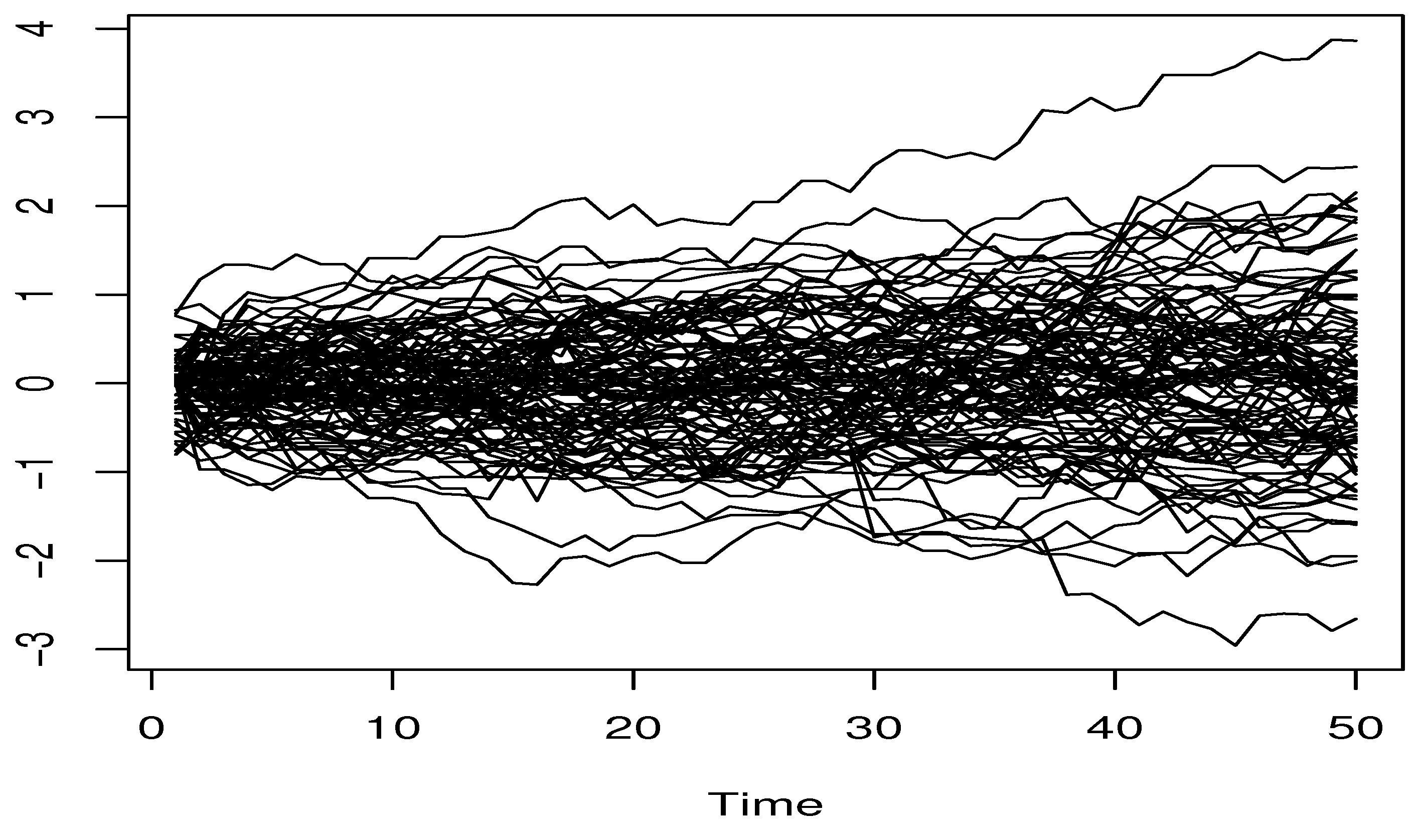
where $w_{\mathbf{i},\mathbf{i}}$ is a known Spatial Weight Matrix (SWM). In fact, this kind of spatio-functional process is obtained using the routine code sim.spARCH in the R-package spGARCH. A  sample of the functional co-variate is plotted in Figure 1.

Recall that the principal feature of the FESR-expectile is its high sensitivity to the outliers. To  measure the impact of this characteristic, we use the routine code ODM in the R-Package OutlierDM to detect the number of outliers in each model. It appears that the first model contains $4\%$ versus $28\%$ for the second one. On the other hand, the spatial-heterogeneity of the data constitutes a second principal issue of our study. The latter is controlled through the parameters $\sigma$, $\varphi$ and the spatial weight matrix $w_{\mathbf{i},\mathbf{i}}$. So, we calculate

$$MSE\left(p\right)={\overline{\mathbf{n}}}^{-1}\sum _{\mathbf{i}\in {\mathbf{I}}_{\mathbf{n}}}{\left(B_{\mathbf{i}}-\widehat{{REA}_p}\left(A_{\mathbf{i}}\right)\right)}^2{1\mathrm{I}}_{B_{\mathbf{i}}>\widehat{{REA}_p}\left(A_{\mathbf{i}}\right)}$$

for various values of the mentioned parameters.

Now, for this empirical study, we choose the smoothing parameter r via the local mean square cross-validation method as in (6). In the sense that the optimization of the mean square rule is performed over a discrete set defined by the $k^{th}$-distance from the location point. The integer number k is obtained from $\{5,10,15,20,25,30,\dots 50\}$. For the kernel $\mathbf{F}$, we use the $\beta$-kernel. Finally, the metric is chosen according to the nature of the functional variable and its smoothing property. It appears that the principal component (pca) metric is more suitable for this type of discontinuous functional regressor.

The simulation results are given in

Table 1. Comparison results.

Model	n1	n2	$\sigma$	$\varphi$	SWM	MSE (0.01)	MSE (0.05)	MSE (0.5)	MSE (0.90)
M1	20	50	0.09	0.03	Queen	0.023	0.018	0.014	0.026
	50	30	0.09	0.03	Bishop	0.034	0.027	0.018	0.032
	20	30	0.79	0.93	Bishop	0.042	0.032	0.026	0.045
	20	50	0.09	0.03	Rook	0.042	0.020	0.018	0.037
	50	30	0.79	0.03	Rook	0.021	0.016	0.022	0.031
M2	20	50	0.09	0.03	Queen	0.045	0.036	0.028	0.044
	50	30	0.09	0.03	Bishop	0.071	0.053	0.026	0.059
	20	30	0.75	0.93	Bishop	0.096	0.052	0.048	0.105
	20	50	0.09	0.03	Rook	0.086	0.054	0.032	0.049
	50	30	0.79	0.03	Rook	0.039	0.025	0.047	0.055

.

We observe that the behavior of the estimator $\widehat{{REA}_p}$ is strongly affected by the different parameters of this study, such as the rate of the outliers and the spatial dependency degree. The high variability of the error between these different situations highlights the importance of the FESR- expectile as a risk-metric. In particular, the MSE varies between $0.018$ and $0.045$ with respect to the spatial level, while the horizontal variability, which describes the sensitivity to the outliers rate, ranges between $0.018$ and $0.095$. These results incorporate the theoretical study, where the convergence rate is strongly affected by the local dependency of the spatio-functional data. In the sense that the computational part proves that the performance of the estimator is strongly impacted by the degree of spatial correlation of the data. Such a conclusion highlights the importance of the expectile-based-shortfall. The latter is very sensitive to the variability or deviation of the data, allowing more reliability in risk detection. This feature makes the expectile-based-shortfall more appropriate as a risk metric than the standard expected shortfall. We point out that the standard expected shortfall is based on the quantile, which is a robust model with low sensitivity to the variability in the risk analysis, because the risk is often located in the extremes. Such a characteristic is not beneficial in risk analysis. Finally, we can say that the estimator $\widehat{{REA}_p}$ is very easy to implement and has good performance according to the nature of the treated data.

5. Real Data Application

After demonstrating the straightforward implementation of the estimator in the last section, we now focus on the applicability of our model to real spatial time series data. More specifically, we compare the performance of the new FESR-expectile $\widehat{{REA}_p}$ to the classical one

$$\widetilde{RE{S}_p}\left(s\right)={\displaystyle \frac{{\sum }_{\mathbf{i}\in {\mathbf{I}}_{\mathbf{n}}}\mathbf{F}(r^{-1}d(\mathfrak{z},A_{\mathbf{i}})\left(aG\left(a^{-1}(\widehat{RVa{R}_p}\left(\mathfrak{z}\right)-B_{\mathbf{i}})\right)+B_{\mathbf{i}}\left(1-H(a^{-1}\left(\widehat{RVa{R}_p}\left(\mathfrak{z}\right)-B_{\mathbf{i}})\right)\right)\right)}{p{\sum }_{\mathbf{i}\in {\mathbf{I}}_{\mathbf{n}}}\mathbf{F}\left(r^{-1}d(\mathfrak{z},A_{\mathbf{i}})\right)}},$$

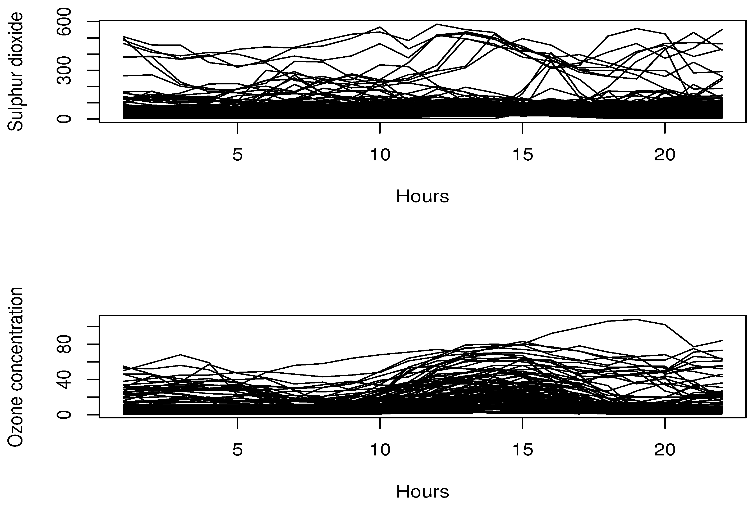
where $G\left(s\right)={\int }_s^{\infty }u\mathbf{F}\left(u\right)$ and $H\left(s\right)={\int }_{-infty}^s\mathbf{F}\left(u\right)du.$ In the previous section, we evaluated the impact of spatial correlation using the ARCH model, which is well-solicited as an appropriate method for fitting the financial time series data. Alternatively, in this part, we employ the FESR-expectile model for another area, specifically in the environmental domain. This application emphasizes the importance and versatility of the FESR model. The environmental domain is a particularly relevant area for risk management, as air quality significantly affects the quality of life. Moreover, the extreme values models have usually been employed to model the risk in this area. Here, we aim to compare the efficiency of the FESR- expectile $\widehat{{REA}_p}$ with the FESR-VaR $\widetilde{RE{S}_p}$ in terms of risk prevention in air quality domain. For this goal, we analyze the air quality data used by [42], which concerns the ozone concentration in Beijing. These data are available on the website https://dataverse.harvard.edu/dataverse/beijing-air (accessed on 8 August 2024). Furthermore, there are many indices of air quality, such as Ozone (O₃), Particulate Matter (PM2.5 and PM10), Nitrogen Dioxide (NO₂), Carbon, and Sulfur Dioxide (SO₂). However, in this section, we concentrate on the ozone quantity (O₃) and sulfur dioxide (SO₂). Recall that the (SO₂) and the ultraviolet rays have a significant impact on the stratospheric ozone. Specifically, we collect the data from 120 monitoring stations in Beijing and we define $A_{\mathbf{i}}$ as the daily curve of SO₂ at the station $\mathbf{i}$ (on 30 December 2016). The response variable $B_{\mathbf{i}}$ represents the total ozone measured the day before at the same station $\mathbf{i}$. The daily curves for the sulphur dioxide are shown in Figure 2.

Now, in order to explore the spatial correlation of the data, we follow the same strategy considered by [43]. This strategy permits us to estimate the spatial trend using the classical regression as follows. Indeed, we define

$${\tilde{A}}_{\mathbf{i}}=r_1\left(\mathbf{i}\right)+A_{\mathbf{i}}\mathrm{and}{\tilde{B}}_{\mathbf{i}}=r_2\left(\mathbf{i}\right)+B_{\mathbf{i}}.$$

Therefore, before  computing the estimators $\widehat{{REA}_p}$ and $\widetilde{RE{S}_p}$, we start by estimating the statistics ${({\widehat{A}}_{\mathbf{i}},{\widehat{B}}_{\mathbf{i}})}_{\mathbf{i}}$. The latter is estimated by

$${\widehat{A}}_{\mathbf{i}}={\tilde{A}}_{\mathbf{i}}-{\widehat{r}}_1\left(\mathbf{i}\right)\mathrm{and}{\widehat{B}}_{\mathbf{i}}={\tilde{B}}_{\mathbf{i}}-{\widehat{r}}_2\left(\mathbf{i}\right),$$

where ${\widehat{r}}_1(.)$ and ${\widehat{r}}_2(.)$ are the kernel estimators of the functions $r_1$ and $r_2$ which are

$${\widehat{m}}_1\left({\mathbf{i}}_0\right)={\displaystyle \frac{{\sum }_{\mathbf{i}\in {\mathbf{I}}_{\mathbf{n}}}{\mathbf{F}}_1(r^{-1}\parallel {\mathbf{i}}_0-\mathbf{i}\parallel )A_{\mathbf{i}}}{{\sum }_{\mathbf{i}\in {\mathbf{I}}_{\mathbf{n}}}{\mathbf{F}}_1(r^{-1}\parallel {\mathbf{i}}_0-\mathbf{i}\parallel )}}(\mathrm{resp}. {\widehat{m}}_2\left({\mathbf{j}}_0\right)={\displaystyle \frac{{\sum }_{\mathbf{j}\in {\mathbf{I}}_{\mathbf{n}}}{\mathbf{F}}_2(r^{-1}\parallel {\mathbf{j}}_0-\mathbf{j}\parallel )B_{\mathbf{j}}}{{\sum }_{\mathbf{i}\in {\mathbf{I}}_{\mathbf{n}}}{\mathbf{F}}_2(r^{-1}\parallel {\mathbf{j}}_0-\mathbf{j}\parallel )}}),$$

where ${\mathbf{F}}_1,{\mathbf{F}}_2$ are kernel functions. Such estimators are obtained using the routine code npreg in the R-package np with ${\mathbf{F}}_1={\mathbf{F}}_2$ being the quadratic kernel. This step is fundamental for spatio-functional data analysis and is referred to as the detrending step. To highlight the potential impact of spatial correlation, we compare our expected shortfall to the standard one in both cases: with or without detrending. Specifically, the estimation with detrending is calculated by ${({\widehat{A}}_{\mathbf{i}},{\widehat{B}}_{\mathbf{i}})}_{\mathbf{i}}$, while in the other case (without detrending), we use the initial observation ${(A_{\mathbf{i}},B_{\mathbf{i}})}_{\mathbf{i}}$ to compute the estimators.

Furthermore, to calculate both estimators, we follow the same procedures used in the simulation section. In other words, we use the $(0,1)$ quadratic kernel and the pca-metric, along with local cross-validation for the bandwidth parameter. The efficiency of both estimators is evaluated by computing

$$MSE\left(p\right)={\overline{\mathbf{n}}}^{-1}\sum _{\mathbf{i}\in {\mathbf{I}}_{\mathbf{n}}}{\left(B_{\mathbf{i}}-\widehat{{\Theta }_p}\left(A_{\mathbf{i}}\right)\right)}^2{1\mathrm{I}}_{B_{\mathrm{i}}>\widehat{{\mathit{REX}}^p}{\left(A_{\mathrm{i}}\right)}^{\prime }}$$

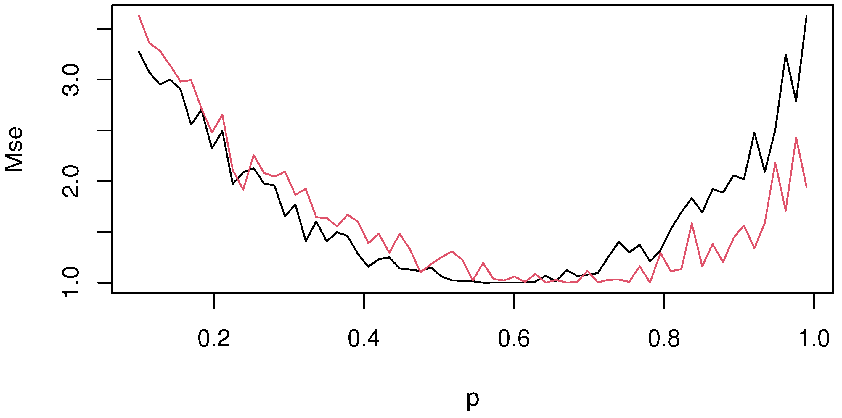
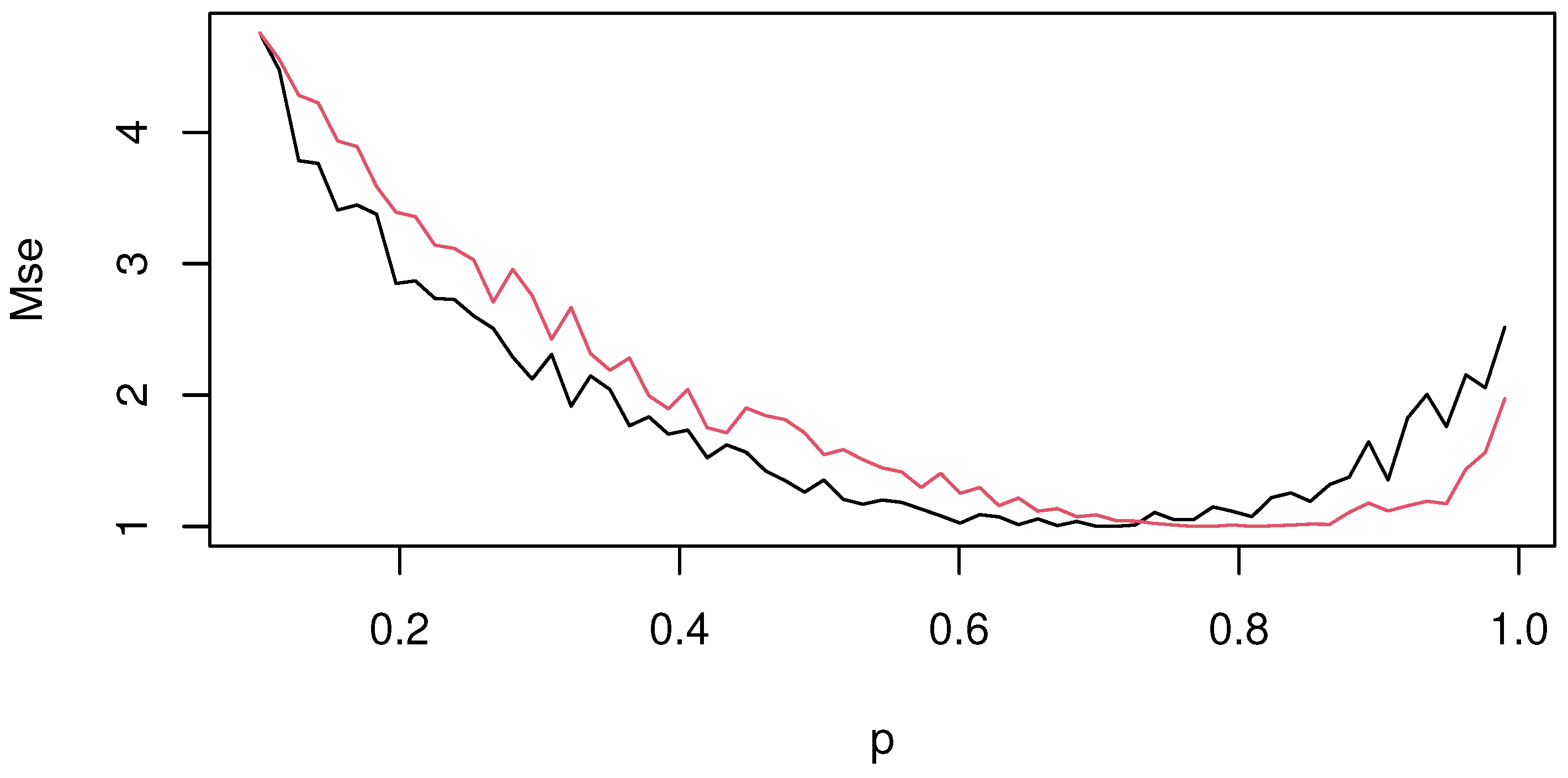
where $\widehat{{\Theta }_p}$ represents $\widehat{{\mathit{REA}}_p}$ or $\widetilde{{\mathit{RES}}_p}$. The values of $MSE\left(\right)$ are evaluated as a function of $p$. In Figure 3 and Figure 4, we show the values of $MSE$ of both estimators $\widehat{{\mathit{REA}}_p}$(black line) and $\widetilde{{\mathit{RES}}_p}$(red line) in both cases (with detrending and without detrending step—see Figure 3 and Figure 4).

The graphs show the superiority of the FESR-expectile regression over the FESR-quantile model. This statement can be confirmed by the position of the black line, which is under the red line in most cases. These results show that the FESR-expectile detects the excessive level of ozone concentration more effectively, even in cases of high variability. This feature is not surprising. The slow variability of the VaR level is due to the robustness of the quantile regression, which reduces its sensitivity to extreme values. Additionally, this advantage seems to be more significant in the detrending step compared to the non-detrending case. This statement can be confirmed using the cover test developed by Bayer and Dimitriadis [44]. This test allows us to examine the goodness-of-fit of our approach. The proposed test is an alternative approach to the procedure introduced by [45] for forecasting. Since the risk prediction differs significantly from standard prediction, we have opted to examine the feasibility of our risk-metric using the Bayer–Dimitriadis test. Specifically, we compare both functional approaches $\widetilde{RE{S}_p}$ and $\widehat{{REA}_p}$ using the routine code esr-backtest from the R-package esrback. We have employed this code with $\alpha =0.05$. Unsurprisingly, the obtained results confirm that both models are significantly good for this risk management issue. Typically, the cover-test gives a p-value of $\widehat{{REA}_p}$ equal to 0.001, compared to 0.004 for the model $\widetilde{RE{S}_p}$.

6. Conclusions and Prospects

In this contribution, we have considered the nonparametric estimation of the FESR-regression-expectile under the spatial structure. We have constructed the functional version of the kernel estimator of this model as a risk-metric. This study covers a more general case of the functional random field. In the theoretical part, we have established the Borell–Contelli convergence under strong spatial mixing assumptions. Such theoretical development provides indispensable mathematical support for the use of the newly developed risk-metric. Additionally, the obtained asymptotic result was derived under general conditions and with the precision of the pointwise convergence rate. The computational part shows the applicability of the estimator and its very easy implementation in practice. Additionally, we applied the new model to an environmental spatio-functional random process. The result confirms the superiority of the FESR-expectile over FESR-VaR. On the other hand, the importance of this contribution can be viewed through several open future directions. For instance, we will address more dependent cases, such as the quasi-associated spatio-functional time series. This situation allows us to control the co-movement of different stock exchanges using weak dependence. The second issue is determining the uniform UNN convergence of the estimator, which will help in resolving the smoothing parameter selection. Furthermore, we can also estimate the model using either the additive or the linear case.

References

1. Cressie, N.A. Statistics for Spatial Data; Wiley: New York, NY, USA, 1993. [Google Scholar]
2. Diggle, P.; Ribeiro, P.J. Model-Based Geostatistics; Springer: New York, NY, USA, 2007. [Google Scholar]
3. Tran, L.T. Kernel density estimation on random fields. J. Multivar. Anal. 1990, 34, 37–53. [Google Scholar] [CrossRef]
4. Lu, Z.; Chen, X. Spatial kernel regression: Weak consistency. Statist. Probab. Lett. 2004, 68, 125–136. [Google Scholar] [CrossRef]
5. Biau, G.; Cadre, B. Nonparametric spatial prediction. Stat. Inference Stoch. Process. 2004, 7, 327–349. [Google Scholar] [CrossRef]
6. García-Soidán, P.H.; Febrero-Bande, M.; González-Manteiga, W. Nonparametric kernel estimation of an isotropic variogram. J. Stat. Plan. Inference 2004, 121, 65–92. [Google Scholar] [CrossRef]
7. Hallin, M.; Lu, Z.; Tran, L.T. Local linear spatial regression. Ann. Stat. 2004, 32, 2469–2500. [Google Scholar] [CrossRef]
8. Carbon, M.; Francq, C.; Tran, L.T. Kernel regression estimation for random fields. J. Stat. Plan. Inference 2007, 137, 778–798. [Google Scholar] [CrossRef]
9. Xu, R.; Wang, J. L1-estimation for spatial nonparametric regression. J. Nonparametr. Stat. 2008, 20, 523–537. [Google Scholar] [CrossRef]
10. Li, J.; Tran, L.T. Nonparametric estimation of conditional expectation. J. Stat. Plan. Inference 2009, 139, 164–175. [Google Scholar] [CrossRef]
11. Dabo-Niang, S.; Yao, A.F. Kernel regression estimation for continuous spatial processes. Math. Meth. Stat. 2007, 16, 298–317. [Google Scholar] [CrossRef]
12. Laksaci, A.; Maref, F. Estimation non paramétrique de quantiles conditionnels pour des variables fonctionnelles spatialement dépendantes. C. R. Math. 2009, 347, 1075–1080. [Google Scholar] [CrossRef]
13. Mohammedi, M.; Bouzebda, S.; Laksaci, A. The consistency and asymptotic normality of the kernel type expectile regression estimator for functional data. J. Multivar. Anal. 2021, 181, 104673. [Google Scholar] [CrossRef]
14. Aneiros, G.; Cao, R.; Fraiman, R.; Genest, C.; Vieu, P. Recent advances in functional data analysis and high-dimensional statistics. J. Multivar. Anal. 2019, 170, 3–9. [Google Scholar] [CrossRef]
15. Almanjahie, I.M.; Bouzebda, S.; Kaid, Z.; Laksaci, A. The local linear functional kNN estimator of the conditional expectile: Uniform consistency in number of neighbors. Metrika 2024, 1–29. [Google Scholar] [CrossRef]
16. Litimein, O.; Laksaci, A.; Ait-Hennani, L.; Mechab, B.; Rachdi, M. Asymptotic normality of the local linear estimator of the functional expectile regression. J. Multivar. Anal. 2024, 202, 105281. [Google Scholar] [CrossRef]
17. Artzner, P.; Delbaen, F.; Eber, J.M.; Heath, D. Coherent measures of risk. Math. Financ. 1999, 9, 203–228. [Google Scholar] [CrossRef]
18. Righi, M.B.; Ceretta, P.S. A comparison of expected shortfall estimation models. J. Econ. Bus. 2015, 78, 14–47. [Google Scholar] [CrossRef]
19. Lazar, E.; Pan, J.; Wang, S. On the estimation of Value-at-Risk and Expected Shortfall at extreme levels. J. Commod. Mark. 2024, 34, 100391. [Google Scholar] [CrossRef]
20. Moutanabbir, K.; Bouaddi, M. A new non-parametric estimation of the expected shortfall for dependent financial losses. J. Stat. Plan. Inference 2024, 232, 106151. [Google Scholar] [CrossRef]
21. Scaillet, O. Nonparametric estimation and sensitivity analysis of expected shortfall. Math. Financ. Int. J. Math. Stat. Financ. Econ. 2004, 14, 115–129. [Google Scholar] [CrossRef]
22. Ferraty, F.; Quintela-Del-Río, A. Conditional VAR and expected shortfall: A new functional approach. Econom. Rev. 2016, 35, 263–292. [Google Scholar] [CrossRef]
23. Ait-Hennani, L.; Kaid, Z.; Laksaci, A.; Rachdi, M. Nonparametric estimation of the expected shortfall regression for quasi-associated functional data. Mathematics 2022, 10, 4508. [Google Scholar] [CrossRef]
24. Waltrup, L.S.; Sobotka, F.; Kneib, T.; Kauermann, G. Expectile and quantile regression—David and Goliath? Stat. Model. 2015, 15, 433–456. [Google Scholar] [CrossRef]
25. Bellini, F.; Di Bernardino, E.D. Risk management with expectiles. Eur. J. Financ. 2017, 23, 487–506. [Google Scholar] [CrossRef]
26. Bellini, F.; Negri, I.; Pyatkova, M. Backtesting VaR and expectiles with realized scores. Stat. Methods Appl. 2019, 28, 119–142. [Google Scholar] [CrossRef]
27. Farooq, M.; Steinwart, I. Learning rates for kernel-based expectile regression. Mach. Learn. 2019, 108, 203–227. [Google Scholar] [CrossRef]
28. Efron, B. Regression percentiles using asymmetric squared error loss. Stat. Sin. 1991, 1, 93–125. [Google Scholar]
29. Sobotka, F.; Kneib, T. Geoadditive expectile regression. Comput. Stat. Data Anal. 2012, 56, 755–767. [Google Scholar] [CrossRef]
30. Jiang, C.; Jiang, M.; Xu, Q.; Huang, X. Expectile regression neural network model with applications. Neurocomputing 2017, 247, 73–86. [Google Scholar] [CrossRef]
31. Daouia, A.; Girard, S.; Stupfler, G. Estimation of tail risk based on extreme expectiles. J. R. Stat. Soc. Ser. B Stat. Methodol. 2018, 80, 263–292. [Google Scholar] [CrossRef]
32. Maume-Deschamps, V.; Rullière, D.; Said, K. Multivariate extensions of expectiles risk measures. Depend. Model. 2017, 5, 20–44. [Google Scholar] [CrossRef]
33. Maume-Deschamps, V.; Rullière, D.; Said, K. Asymptotics multivariate expectiles. arXiv 2018, arXiv:1704.07152v2. [Google Scholar]
34. Girard, S.; Stupfler, G.; Usseglio-Carleve, A. Functional estimation of extreme conditional expectiles. Econom. Stat. 2022, 21, 131–158. [Google Scholar] [CrossRef]
35. Goia, A.; Vieu, P. An introduction to recent advances in high/infinite dimensional statistics. J. Multivar. Anal. 2016, 170, 1–6. [Google Scholar] [CrossRef]
36. Yu, D.; Pietrosanu, M.; Mizera, I.; Jiang, B.; Kong, L.; Tu, W. Functional Linear Partial Quantile Regression with Guaranteed Convergence for Neuroimaging Data Analysis. Stat. Biosci. 2024, 1–17. [Google Scholar] [CrossRef]
37. Di Bernardino, E.; Laloe, T.; Pakzad, C. Estimation of extreme multivariate expectiles with functional covariates. J. Multivar. Anal. 2024, 202, 105292. [Google Scholar] [CrossRef]
38. Guyon, X. Estimation d’un champ par pseudo-vraisemblance conditionnelle: Etude asymptotique et application au cas Markovien. In Proceedings of the Sixth Franco-Belgian Meeting of Statisticians, Bruxelles, Belguim, 14–15 November 1987. [Google Scholar]
39. Ferraty, F.; Vieu, P. Nonparametric Functional Data Analysis: Theory and Practice; Springer Series in Statistics; Springer: New York, NY, USA, 2006. [Google Scholar]
40. Li, W.V.; Shao, Q.M. Gaussian processes: Inequalities, small ball probabilities and applications. Hanbook Stat. 2001, 19, 533–597. [Google Scholar]
41. Liebscher, E. Estimation of the density and the regression function under mixing conditions. Stat. Decis. 2001, 19, 9–26. [Google Scholar] [CrossRef]
42. Rachdi, M.; Laksaci, A.; Al-Kandari, N.M. Expectile regression for spatial functional data analysis (sFDA). Metrika 2022, 85, 627–655. [Google Scholar] [CrossRef]
43. Hallin, M.; Lu, Z.; Yu, K. Local linear spatial quantile regression. Bernoulli 2009, 15, 659–686. [Google Scholar] [CrossRef]
44. Bayer, S.; Dimitriadis, T. Regression-Based Expected Shortfall Backtesting. J. Financ. Econom. 2022, 20, 437–471. [Google Scholar] [CrossRef]
45. Hassani, H.; Silva, E.S. A Kolmogorov-Smirnov based test for comparing the predictive accuracy of two sets of forecasts. Econometrics 2015, 3, 590–609. [Google Scholar] [CrossRef]
Figure 1. The ARCH process for α = 0.05 and ρ = 0.8 .
Axioms 13 00678 g001
Figure 2. The SO2 and O3 daily curves.
Axioms 13 00678 g002
Figure 3. Comparison of the M S E values between FESR-expectile and FESR-VaR without detrending cases. The black line represents R E A p ^ , and the red line represents R E S p ˜ .
Axioms 13 00678 g003
Figure 4. Comparison of the M S E values between FESR-expectile and FESR-VaR with detrending cases. The black line represents R E A p ^ , and the red line represents R E S p ˜ .
Axioms 13 00678 g004