Calibrating and Visualizing Some Bootstrap Confidence Regions

Abstract

When the bootstrap sample size is moderate, bootstrap confidence regions tend to have undercoverage. Improving the coverage is known as calibrating the confidence region. Consider testing $H_0:\mathit{\theta }={\mathit{\theta }}_0$ versus $H_1:\mathit{\theta }\ne {\mathit{\theta }}_0$. We reject $H_0$ only if ${\mathit{\theta }}_0$ is not contained in a large-sample 95% confidence region. If the confidence region has 3% undercoverage for the data set sample size, then the type I error is 8% instead of the nominal 5%. Hence, calibrating confidence regions is also useful for testing hypotheses. Several bootstrap confidence regions are also prediction regions for a future value of a bootstrap statistic. A new bootstrap confidence region uses a simple prediction region calibration technique to improve the coverage. The DD plot for visualizing prediction regions can also be used to visualize some bootstrap confidence regions.

1. Introduction

When the bootstrap sample size B is small or moderate, bootstrap confidence regions, including bootstrap confidence intervals, tend to have undercoverage: the probability that the confidence region contains the $p\times 1$ parameter vector $\mathit{\theta }$ is less than the nominal large-sample coverage probability $1-\delta$. Then, coverage can be increased by increasing the nominal coverage of the large-sample bootstrap confidence region. For example, if the undercoverage of the nominal large-sample 95% bootstrap confidence region with $B=1000$ is 2%, the coverage is increased to 97%. This procedure is known as calibrating the confidence region. Calibration tends to be difficult since the amount of undercoverage is usually unknown. This paper provides a simple method for improving the coverage and provides a method for visualizing some bootstrap confidence regions.

Using correction factors for large-sample confidence intervals, tests, prediction intervals, prediction regions, and confidence regions improves the coverage performance for a moderate sample size n. If confidence regions are used for hypothesis testing, then this calibration reduces the type I error. For a random variable X, let $P(X\le x_{1-\delta })=1-\delta .$ Note that correction factors $b_n\to 1$ as $n\to \infty$ are used in large-sample confidence intervals and large-sample tests if the limiting distribution is $Z\sim N(0,1)$ or $X\sim {\chi }_k^2$, but a $t_{d_n}$ or $k{F}_{k,d_n}$ cutoff is used: $t_{d_n,1-\delta }=(t_{d_n,1-\delta }/z_{1-\delta })z_{1-\delta }$ with $b_n=t_{d_n,1-\delta }/z_{1-\delta }\to 1$ and $k{F}_{k,d_n,1-\delta }=(k{F}_{k,d_n,1-\delta }/{\chi }_{k,1-\delta }^2){\chi }_{k,1-\delta }^2$ with $b_n=k{F}_{k,d_n,1-\delta }/{\chi }_{k,1-\delta }^2\to 1$ if $d_n\to \infty$ as $n\to \infty$. For moderate n, the test or confidence interval with the correction factor $b_n>1$ has better level or coverage than the test or confidence interval that does not use the correction factor, in that the simulated level or coverage is closer to the nominal level or coverage.

Sometimes, the test statistic has a $t_{d_n}$ or $F_{k,d_n}$ distribution under normality, but the test statistic (possibly scaled by multiplying by k) is asymptotically normal or asymptotically ${\chi }_k^2$ for a large class of distributions. The t test and t confidence interval for the sample mean are examples where the asymptotic normality holds by the central limit theorem. Many F tests for linear models, experimental design models, and multivariate analyses also satisfy $k{F}_0\stackrel{D}{\to }{\chi }_k^2$ as $n\to \infty$, where $F_0$ is the test statistic. See, for example, Olive (2017) [1].

Section 1.1 reviews prediction intervals, prediction regions, confidence intervals, and confidence regions. Several of these methods use correction factors to improve the coverage, and several bootstrap confidence intervals and regions are obtained by applying prediction intervals and regions to the bootstrap sample. Section 1.2 reviews a bootstrap theorem and shows that some bootstrap confidence regions are asymptotically equivalent.

Section 2.1 gives a new bootstrap confidence region with a simple correction factor, while Section 2.2 shows how to visualize some bootstrap confidence regions. Section 3 presents some simulation results.

1.1. Prediction Regions and Confidence Regions

Consider predicting a future test value $Y_f$ given past training data $Y_1,\dots ,Y_n$, where $Y_1,\dots ,Y_n,Y_f$ are independent and identically distributed (iid). A large-sample $100(1-\delta )\%$ prediction interval (PI) for $Y_f$ is $[L_n,U_n]$, where the coverage $P(L_n\le Y_f\le U_n)=1-{\delta }_n$ is eventually bounded below by $1-\delta$ as $n\to \infty$. We often want $1-{\delta }_n\to 1-\delta$ as $n\to \infty$. A large-sample $100(1-\delta )\%$ PI is asymptotically optimal if it has the shortest asymptotic length: the length of $[{\widehat{L}}_n,{\widehat{U}}_n]$ converges to $U_s-L_s$ as $n\to \infty$, where $[L_s,U_s]$ is the population shorth, the shortest interval covering at least $100(1-\delta )\%$ of the mass.

Let the data $\mathit{Y}={(Y_1,\dots ,Y_n)}^T$ have joint probability density function or probability mass function $f\left(\mathit{y}\right|\theta )$ with parameter space $\Theta$ and support $\mathcal{Y}$. Let $L_n=L_n\left(\mathit{Y}\right)$ and $U_n=U_n\left(\mathit{Y}\right)$ be statistics such that $L_n\left(\mathit{y}\right)\le U_n\left(\mathit{y}\right),$$\forall \mathit{y}\in \mathcal{Y}.$ Then, the interval $[L_n\left(\mathit{y}\right),U_n\left(\mathit{y}\right)]$ is a large-sample $100(1-\delta )\%$ confidence interval (CI) for $\theta$ if

$$P_{\theta }(L_n\left(\mathit{Y}\right)\le \theta \le U_n\left(\mathit{Y}\right))$$

is eventually bounded below by $1-\delta$ for all $\theta \in \Theta$ as the sample size $n\to \infty .$

Consider predicting a $p\times 1$ future test value ${\mathit{x}}_f$, given past training data ${\mathit{x}}_1,\dots ,{\mathit{x}}_n$, where ${\mathit{x}}_1,\dots ,{\mathit{x}}_n,{\mathit{x}}_f$ are iid. A large-sample $100(1-\delta )\%$ prediction region is a set ${\mathcal{A}}_n$ such that $P({\mathit{x}}_f\in {\mathcal{A}}_n)$ is eventually bounded below by $1-\delta$ as $n\to \infty$. A prediction region is asymptotically optimal if its volume converges in probability to the volume of the minimum volume covering region or the highest density region of the distribution of ${\mathit{x}}_f.$

A large-sample $100(1-\delta )\%$ confidence region for a $p\times 1$ vector of parameters $\mathit{\theta }$ is a set ${\mathcal{A}}_n$ such that $P(\mathit{\theta }\in {\mathcal{A}}_n)$ is eventually bounded below by $1-\delta$ as $n\to \infty .$ For testing $H_0:\mathit{\theta }={\mathit{\theta }}_0$ versus $H_1:\mathit{\theta }\ne {\mathit{\theta }}_0$, we fail to reject $H_0$ if ${\mathit{\theta }}_0$ is in the confidence region and reject $H_0$ if ${\mathit{\theta }}_0$ is not in the confidence region.

For prediction intervals, let $Y_{\left(1\right)}\le Y_{\left(2\right)}\le \dots \le Y_{\left(n\right)}$ be the order statistics of the training data. Open intervals need more regularity conditions than closed intervals. For the following prediction interval, if the open interval $(Y_{\left(k_1\right)},Y_{\left(k_2\right)})$ was used, we would need to add the regularity condition that the population percentiles $Y_{\delta /2}$ and $Y_{1-\delta /2}$ are continuity points of the cumulative distribution function $F_Y\left(y\right).$ See Frey (2013) [2] for references.

Let $k_1=\lceil n\delta /2\rceil$ and $k_2=\lceil n(1-\delta /2)\rceil$, where $0<\delta <1$. A large-sample $100(1-\delta )\%$ percentile prediction interval for $Y_f$ is

$$[Y_{\left(k_1\right)},Y_{\left(k_2\right)}].$$

(1)

The bootstrap percentile confidence interval given by Equation (2) is obtained by applying the percentile prediction interval (1) to the bootstrap sample $T_1^{*},\dots ,T_B^{*}$, where $T=T_n$ is a test statistic. See Efron (1982) [3].

A large-sample $100(1-\delta )\%$ bootstrap percentile confidence interval for $\theta$ is an interval $[T_{\left(k_L\right)}^{*},T_{\left(k_U\right)}^{*}]$ containing $\approx \lceil B(1-\delta )\rceil$ of the $T_i^{*}$. Let $k_1=\lceil B\delta /2\rceil$ and $k_2=\lceil B(1-\delta /2)\rceil$. A common choice is

$$[T_{\left(k_1\right)}^{*},T_{\left(k_2\right)}^{*}].$$

(2)

The shorth (c) estimator of the population shorth is useful for making asymptotically optimal prediction intervals. For a large-sample $100(1-\delta )\%$ PI, the nominal coverage is $100(1-\delta )\%$. Undercoverage occurs if the actual coverage is below the nominal coverage. For example, if the actual coverage is 0.93 for a large-sample 95% PI, then the undercoverage is 0.02. Consider intervals that contain c cases $[Y_{\left(1\right)},Y_{\left(c\right)}],[Y_{\left(2\right)},Y_{(c+1)}],\dots ,[Y_{(n-c+1)},Y_{\left(n\right)}]$. Compute $Y_{\left(c\right)}-Y_{\left(1\right)},Y_{(c+1)}-Y_{\left(2\right)},\dots ,Y_{\left(n\right)}-Y_{(n-c+1)}$. Then, the estimator shorth (c) $=[Y_{\left(s\right)},Y_{(s+c-1)}]$ is the interval with the shortest length. The shorth (c) interval is a large-sample $100(1-\delta )\%$ PI if $c/n\to 1-\delta$ as $n\to \infty$ that often has the asymptotically shortest length. Let $k_n=\lceil n(1-\delta )\rceil$. Frey (2013) [2] showed that for large $n\delta$ and iid data, the large-sample $100(1-\delta )\%$ shorth ($k_n$) prediction interval has maximum undercoverage ≈$1.12\sqrt{\delta /n}$, and then used the large-sample $100(1-\delta )\%$ PI shorth (c) =

$$[Y_{\left(s\right)},Y_{(s+c-1)}]\mathit{w}ithc=min(n,\lceil n[1-\delta +1.12\sqrt{\delta /n}]\rceil ).$$

(3)

The shorth confidence interval is a practical implementation of Hall’s (1988) [4] shortest bootstrap percentile interval based on all possible bootstrap samples, and is obtained by applying shorth PI (3) to the bootstrap sample $T_1^{*},\dots ,T_B^{*}.$ See Pelawa Watagoda and Olive (2021) [5]. The large-sample $100(1-\delta )\%$ shorth (c) CI =

$$[T_{\left(s\right)}^{*},T_{(s+c-1)}^{*}]\mathit{w}herec=min(B,\lceil B[1-\delta +1.12\sqrt{\delta /B}]\rceil ).$$

(4)

To describe Olive’s (2013) [6] nonparametric prediction region, Mahalanobis distances will be useful. Let the $p\times 1$ column vector $T=T_n$ be a multivariate location estimator, and let the $p\times p$ symmetric positive definite matrix ${\mathit{C}}_n$ be a dispersion estimator. Then, the ith squared sample Mahalanobis distance is the scalar

$$D_i^2=D_i^2(T_n,{\mathit{C}}_n)=D_{{\mathit{x}}_i}^2(T_n,{\mathit{C}}_n)={({\mathit{x}}_i-T_n)}^T{\mathit{C}}_n^{-1}({\mathit{x}}_i-T_n)$$

(5)

for each observation ${\mathit{x}}_i,$ where $i=1,\dots ,n$. Notice that the Euclidean distance of ${\mathit{x}}_i$ from the estimate of center T is $D_i(T_n,{\mathit{I}}_p)$, where ${\mathit{I}}_p$ is the $p\times p$ identity matrix. The classical Mahalanobis distance $D_i$ uses $(T_n,{\mathit{C}}_n)=(\overline{\mathit{x}},\mathit{S})$, the sample mean, and sample covariance matrix, where

$$\overline{\mathit{x}}={\displaystyle \frac{1}{n}}\sum _{i=1}^n{\mathit{x}}_i\mathrm{and}\mathit{S}={\displaystyle \frac{1}{\mathrm{n}-1}}\sum _{\mathrm{i}=1}^{\mathrm{n}}({\mathit{x}}_{\mathrm{i}}-\overline{\mathit{x}}){({\mathit{x}}_{\mathrm{i}}-\overline{\mathit{x}})}^{\mathrm{T}}.$$

(6)

Let the $p\times 1$ location vector be $\mathit{\mu }$, which is often the population mean, and let the $p\times p$ dispersion matrix be $\mathbf{\Sigma }$, which is often the population covariance matrix. If x is a random vector, then the population squared Mahalanobis distance is

$$D_{\mathit{x}}^2(\mathit{\mu },\mathbf{\Sigma })={(\mathit{x}-\mathit{\mu })}^T{\mathbf{\Sigma }}^{-1}(\mathit{x}-\mathit{\mu }).$$

(7)

Like prediction intervals, prediction regions often need correction factors. For iid data from a distribution with a $p\times p$ nonsingular covariance matrix, it was found that the simulated maximum undercoverage of prediction region (9) without the correction factor was about 0.05 when $n=20p$. Hence, correction factor (8) is used to obtain better coverage for small n. Let $q_n=min(1-\delta +0.05,1-\delta +p/n)$ for $\delta >0.1$ and

$$q_n=min(1-\delta /2,1-\delta +10\delta p/n),\mathrm{otherwise}.$$

(8)

If $1-\delta <0.999$ and $q_n<1-\delta +0.001$, set $q_n=1-\delta$. Let $D_{\left(U_n\right)}$ be the $100q_n$th sample quantile of the $D_i$, where $i=1,\dots ,n$. Olive (2013) [6] suggests that $n\ge 50p$ may be needed for the following prediction region to have a good volume, and $n\ge 20p$ for good coverage. Of course, for any n, there are distributions that will have severe undercoverage.

The large-sample $100(1-\delta )\%$ nonparametric prediction region for a future value ${\mathit{x}}_f$ given iid data ${\mathit{x}}_1,\dots ,{\mathit{x}}_n$ is

$$\{\mathit{z}:{(\mathit{z}-\overline{\mathit{x}})}^T{\mathit{S}}^{-1}(\mathit{z}-\overline{\mathit{x}})\le D_{\left(U_n\right)}^2\}=\{\mathit{z}:D_{\mathit{z}}^2(\overline{\mathit{x}},\mathit{S})\le D_{\left(U_n\right)}^2\}.$$

(9)

Olive’s (2017, 2018) [1,7] prediction region method confidence region applies prediction region (9) to the bootstrap sample. Let the bootstrap sample be $T_1^{*},\dots ,T_B^{*}$. Let ${\displaystyle {\overline{T}}^{*}}$ and ${\displaystyle {\mathit{S}}_T^{*}}$ be the sample mean and sample covariance matrix of the bootstrap sample.

The large-sample $100(1-\delta )\%$ prediction region method confidence region for $\mathit{\theta }$ is

$$\{\mathit{w}:{(\mathit{w}-{\overline{T}}^{*})}^T{\left[{\mathit{S}}_T^{*}\right]}^{-1}(\mathit{w}-{\overline{T}}^{*})\le D_{\left(U_B\right)}^2\}=\{\mathit{w}:D_{\mathit{w}}^2({\overline{T}}^{*},{\mathit{S}}_T^{*})\le D_{\left(U_B\right)}^2\}$$

(10)

where the cutoff $D_{\left(U_B\right)}^2$ is the $100q_B$th sample quantile of the $D_i^2={(T_i^{*}-{\overline{T}}^{*})}^T{\left[{\mathit{S}}_T^{*}\right]}^{-1}(T_i^{*}-{\overline{T}}^{*})$ for $i=1,\dots ,B$. Note that the corresponding test for $H_0:\mathit{\theta }={\mathit{\theta }}_0$ rejects $H_0$ if ${({\overline{T}}^{*}-{\mathit{\theta }}_0)}^T{\left[{\mathit{S}}_T^{*}\right]}^{-1}({\overline{T}}^{*}-{\mathit{\theta }}_0)>D_{\left(U_B\right)}^2$.

Olive’s (2017, 2018) [1,7] large-sample $100(1-\delta )\%$ modification of Bickel and Ren’s (2001) [8] confidence region is

$$\{\mathit{w}:{(\mathit{w}-T_n)}^T{\left[{\mathit{S}}_T^{*}\right]}^{-1}(\mathit{w}-T_n)\le D_{\left(U_{BT}\right)}^2\}=\{\mathit{w}:D_{\mathit{w}}^2(T_n,{\mathit{S}}_T^{*})\le D_{\left(U_{BT}\right)}^2\}$$

(11)

where the cutoff $D_{\left(U_{BT}\right)}^2$ is the $100q_B$th sample quantile of the $D_i^2={(T_i^{*}-T_n)}^T{\left[{\mathit{S}}_T^{*}\right]}^{-1}(T_i^{*}-T_n).$ Note that the corresponding test for $H_0:\mathit{\theta }={\mathit{\theta }}_0$ rejects $H_0$ if ${(T_n-{\mathit{\theta }}_0)}^T{\left[{\mathit{S}}_T^{*}\right]}^{-1}(T_n-{\mathit{\theta }}_0)>D_{\left(U_{BT}\right)}^2$.

Shift region (9) to have center $T_n$, or equivalently, to change the cutoff of region (11) to $D_{\left(U_B\right)}^2$ to obtain Pelawa Watagoda and Olive’s (2021) [5] large-sample $100(1-\delta )\%$ hybrid confidence region,

$$\{\mathit{w}:{(\mathit{w}-T_n)}^T{\left[{\mathit{S}}_T^{*}\right]}^{-1}(\mathit{w}-T_n)\le D_{\left(U_B\right)}^2\}=\{\mathit{w}:D_{\mathit{w}}^2(T_n,{\mathit{S}}_T^{*})\le D_{\left(U_B\right)}^2\}.$$

(12)

Note that the corresponding test for $H_0:\mathit{\theta }={\mathit{\theta }}_0$ rejects $H_0$ if ${(T_n-{\mathit{\theta }}_0)}^T{\left[{\mathit{S}}_T^{*}\right]}^{-1}(T_n-{\mathit{\theta }}_0)>D_{\left(U_B\right)}^2$.

Rajapaksha and Olive (2024) [9] gave the following two confidence regions. The names of these confidence regions were chosen since they are similar to Bickel and Ren’s and the prediction region method’s confidence regions.

The large-sample $100(1-\delta )\%$ BR confidence region is

$$\{\mathit{w}:n{(\mathit{w}-T_n)}^T{\mathit{C}}_n^{-1}(\mathit{w}-T_n)\le D_{\left(U_{BT}\right)}^2\}=\{\mathit{w}:D_{\mathit{w}}^2(T_n,{\mathit{C}}_n/n)\le D_{\left(U_{BT}\right)}^2\}$$

(13)

where the cutoff $D_{\left(U_{BT}\right)}^2$ is the $100q_B$th sample quantile of the $D_i^2=n{(T_i^{*}-T_n)}^T{\mathit{C}}_n^{-1}(T_i^{*}-T_n)$. Note that the corresponding test for $H_0:\mathit{\theta }={\mathit{\theta }}_0$ rejects $H_0$ if $n{(T_n-{\mathit{\theta }}_0)}^T{\mathit{C}}_n^{-1}(T_n-{\mathit{\theta }}_0)>D_{\left(U_{BT}\right)}^2$.

The large-sample $100(1-\delta )\%$ PR confidence region for $\mathit{\theta }$ is

$$\{\mathit{w}:n{(\mathit{w}-{\overline{T}}^{*})}^T{\mathit{C}}_n^{-1}(\mathit{w}-{\overline{T}}^{*})\le D_{\left(U_B\right)}^2\}=\{\mathit{w}:D_{\mathit{w}}^2({\overline{T}}^{*},{\mathit{C}}_n/n)\le D_{\left(U_B\right)}^2\}$$

(14)

where $D_{\left(U_B\right)}^2$ is the $100q_B$th sample quantile of the $D_i^2=n{(T_i^{*}-{\overline{T}}^{*})}^T{\mathit{C}}_n^{-1}(T_i^{*}-{\overline{T}}^{*})$ for $i=1,\dots ,B$. Note that the corresponding test for $H_0:\mathit{\theta }={\mathit{\theta }}_0$ rejects $H_0$ if $n{({\overline{T}}^{*}-{\mathit{\theta }}_0)}^T{\mathit{C}}_n^{-1}({\overline{T}}^{*}-{\mathit{\theta }}_0)>D_{\left(U_B\right)}^2$.

Assume that ${\mathit{x}}_1,\dots ,{\mathit{x}}_n,{\mathit{x}}_f$ are iid $N_p(\mathit{\mu },{\mathbf{\Sigma }}_{\mathit{x}})$. Then, Chew’s (1966) [10] large-sample $100(1-\delta )\%$ classical prediction region for multivariate normal data is

$$\{\mathit{z}:D_{\mathit{z}}^2(\overline{\mathit{x}},\mathit{S})\le {\chi }_{p,1-\delta }^2\}.$$

(15)

The next bootstrap confidence region is similar to what would be obtained if the classical prediction region (15) for multivariate normal data was applied to the bootstrap sample. The large-sample $100(1-\delta )\%$ standard bootstrap confidence region for $\mathit{\theta }$ is

$$\{\mathit{w}:{(\mathit{w}-T_n)}^T{\left[{\mathit{S}}_T^{*}\right]}^{-1}(\mathit{w}-T_n)\le D_{1-\delta }^2\}=\{\mathit{w}:D_{\mathit{w}}^2(T_n,{\mathit{S}}_T^{*})\le D_{1-\delta }^2\}$$

(16)

where $D_{1-\delta }^2={\chi }_{p,1-\delta }^2$ or $D_{1-\delta }^2=p{F}_{p,d_n,1-\delta }$, where $d_n\to \infty$ as $n\to \infty$.

If $p=1$, then a hyperellipsoid is an interval, and confidence intervals are special cases of confidence regions. Suppose the parameter of interest is $\theta$, and there is a bootstrap sample $T_1^{*},\dots ,T_B^{*}$ where the statistic $T_n$ is an estimator of $\theta$ based on a sample of size n. Let $a_i=|T_i^{*}-{\overline{T}}^{*}|$ and let $b_i=|T_i^{*}-T_n|.$ Let ${\overline{T}}^{*}$ and $S_T^{2*}$ be the sample mean and variance of $T_i^{*}$. Then, the squared Mahalanobis distance $D_{\theta }^2={(\theta -{\overline{T}}^{*})}^2/S_T^{*2}\le D_{\left(U_B\right)}^2$ is equivalent to $\theta \in [{\overline{T}}^{*}-S_T^{*}{D}_{\left(U_B\right)},{\overline{T}}^{*}+S_T^{*}{D}_{\left(U_B\right)}]=[{\overline{T}}^{*}-a_{\left(U_B\right)},{\overline{T}}^{*}+a_{\left(U_B\right)}]$, which is an interval centered at ${\overline{T}}^{*}$ just long enough to cover $U_B$ of the $T_i^{*}$. Efron (2014) [11] used a similar large-sample $100(1-\delta )\%$ confidence interval assuming that ${\overline{T}}^{*}$ is asymptotically normal. Then, the large-sample $100(1-\delta )\%$ PR CI is $[{\overline{T}}^{*}-a_{\left(U_B\right)},{\overline{T}}^{*}+a_{\left(U_B\right)}].$ The large-sample $100(1-\delta )\%$ BR CI is $[T_n-b_{\left(U_{BT}\right)},T_n+b_{\left(U_{BT}\right)}]$, which is an interval centered at $T_n$ just long enough to cover $U_{BT}$ of the $T_i^{*}$. The large-sample $100(1-\delta )\%$ hybrid CI is $[T_n-a_{\left(U_B\right)},T_n+a_{\left(U_B\right)}]$.

The following prediction region will be used to develop a new correction factor for bootstrap confidence regions. See Section 2.1. Data splitting divides the training data ${\mathit{x}}_1,\dots ,{\mathit{x}}_n$ into two sets: H and the validation set V, where H has $n_H$ of the cases and V has the remaining $n_V=n-n_H$ cases $i_1,\dots ,i_{n_V}$.

The estimator $(T_H,{\mathit{C}}_H)$ is computed using data set H. Then, the squared validation distances $D_j^2=D_{{\mathit{x}}_{i_j}}^2(T_H,{\mathit{C}}_H)={({\mathit{x}}_{i_j}-T_H)}^T{\mathit{C}}_H^{-1}({\mathit{x}}_{i_j}-T_H)$ are computed for the $j=1,\dots ,n_V$ cases in the validation set V. Let $D_{\left(U_V\right)}^2$ be the $U_V$th order statistic of the $D_j^2$, where

$$U_V=min(n_V,\lceil (n_V+1)(1-\delta )\rceil ).$$

(17)

Haile, Zhang, and Olive’s (2024) [12] large-sample $100(1-\delta )\%$ data splitting prediction region for ${\mathit{x}}_f$ is

$$\{\mathit{z}:D_{\mathit{z}}^2(T_H,{\mathit{C}}_H)\le D_{\left(U_V\right)}^2\}.$$

(18)

1.2. Some Confidence Region Theories

Some large-sample theories for bootstrap confidence regions are given in the references in Section 1.1. The following theorem of Pelawa Watagoda and Olive (2021) [5] and its proof are useful.

Theorem 1. 

(a) Suppose as $n\to \infty$, (i) $\sqrt{n}(T_n-\mathit{\theta })\stackrel{D}{\to }\mathit{u}$, and (ii) $\sqrt{n}(T_i^{*}-T_n)\stackrel{D}{\to }\mathit{u}$ with $E\left(\mathit{u}\right)=0$ and $\mathrm{Cov}\left(\mathit{u}\right)={\mathbf{\Sigma }}_{\mathit{u}}$. Then, (iii) $\sqrt{n}({\overline{T}}^{*}-\mathit{\theta })\stackrel{D}{\to }\mathit{u}$, (iv) $\sqrt{n}(T_i^{*}-{\overline{T}}^{*})\stackrel{D}{\to }\mathit{u}$, and (v) $\sqrt{n}({\overline{T}}^{*}-T_n)\stackrel{P}{\to }0$.

(b) Then, the prediction region method gives a large-sample confidence region for $\mathit{\theta }$ provided that $B\to \infty$ and the sample percentile ${\widehat{D}}_{1-\delta }^2$ of the $D_{T_i^{*}}^2({\overline{T}}^{*},{\mathit{S}}_T^{*})=\sqrt{n}{(T_i^{*}-{\overline{T}}^{*})}^T{\left(n{\mathit{S}}_T^{*}\right)}^{-1}\sqrt{n}(T_i^{*}-{\overline{T}}^{*})$ is a consistent estimator of the percentile $D_{n,1-\delta }^2$ of the random variable $D_{\mathit{\theta }}^2({\overline{T}}^{*},{\mathit{S}}_T^{*})=\sqrt{n}{(\mathit{\theta }-{\overline{T}}^{*})}^T{\left(n{\mathit{S}}_T^{*}\right)}^{-1}\sqrt{n}(\mathit{\theta }-{\overline{T}}^{*})$ in that ${\widehat{D}}_{1-\delta }^2-D_{n,1-\delta }^2\stackrel{P}{\to }0.$

Proof. 

With respect to the bootstrap sample, $T_n$ is a constant, and the $\sqrt{n}(T_i^{*}-T_n)$ are iid for $i=1,\dots ,B$. Fix B. Then,

$$\left[\begin{array}{c}\sqrt{n}(T_1^{*}-T_n)\\ ⋮\\ \sqrt{n}(T_B^{*}-T_n)\end{array}\right]\stackrel{D}{\to }\left[\begin{array}{c}{v}_1\\ ⋮\\ v_B\end{array}\right]$$

where the $v_i$ are iid with the same distribution as u. For fixed B, the average of the $\sqrt{n}(T_i^{*}-T_n)$ is

$$\sqrt{n}({\overline{T}}^{*}-T_n)\stackrel{D}{\to }{\displaystyle \frac{1}{B}}\sum _{i=1}^B{v}_i\sim A{N}_g\left(\mathbf{0},{\displaystyle \frac{{\mathbf{\Sigma }}_{\mathit{u}}}{B}}\right)$$

by the Continuous Mapping Theorem, where $\mathit{z}\sim A{N}_g(\mathbf{0},\mathbf{\Sigma })$ is an asymptotic multivariate normal approximation. Note that if $\mathit{u}\sim N_g(\mathbf{0},{\mathbf{\Sigma }}_{\mathit{u}})$, then

$$\sqrt{n}({\overline{T}}^{*}-T_n)\stackrel{D}{\to }{N}_g\left(\mathbf{0},{\displaystyle \frac{{\mathbf{\Sigma }}_{\mathit{u}}}{B}}\right).$$

Hence, as $B\to \infty$, $\sqrt{n}({\overline{T}}^{*}-T_n)\stackrel{P}{\to }\mathbf{0},$ and (iii), (iv), and (v) hold. Hence, (b) follows.    □

Under regularity conditions, Bickel and Ren (2001), Olive (2017, 2018), and Pelawa Watagoda and Olive (2021) [1,5,7,8] proved that (10), (11), and (12) are large-sample confidence regions. For Theorem 1, usually (i) and (ii) are proven using large-sample theory. Then,

$$D_1^2=D_{T_i^{*}}^2({\overline{T}}^{*},{\mathit{C}}_n/n)=\sqrt{n}{(T_i^{*}-{\overline{T}}^{*})}^T{\mathit{C}}_n^{-1}\sqrt{n}(T_i^{*}-{\overline{T}}^{*}),$$

$$D_2^2=D_{\mathit{\theta }}^2(T_n,{\mathit{C}}_n/n)=\sqrt{n}{(T_n-\mathit{\theta })}^T{\mathit{C}}_n^{-1}\sqrt{n}(T_n-\mathit{\theta }),$$

$$D_3^2=D_{\mathit{\theta }}^2({\overline{T}}^{*},{\mathit{C}}_n/n)=\sqrt{n}{({\overline{T}}^{*}-\mathit{\theta })}^T{\mathit{C}}_n^{-1}\sqrt{n}({\overline{T}}^{*}-\mathit{\theta }),\mathrm{and}$$

$$D_4^2=D_{T_i^{*}}^2(T_n,{\mathit{C}}_n/n)=\sqrt{n}{(T_i^{*}-T_n)}^T{\mathit{C}}_n^{-1}\sqrt{n}(T_i^{*}-T_n),$$

are well behaved. If ${\mathit{C}}_n^{-1}\stackrel{P}{\to }{\mathit{C}}^{-1},$ then $D_j^2\stackrel{D}{\to }{D}^2={\mathit{u}}^T{\mathit{C}}^{-1}\mathit{u}$, and (13) and (14) are large-sample confidence regions. If ${\mathit{C}}_n^{-1}$ is “not too ill conditioned," then $D_j^2\approx {\mathit{u}}^T{\mathit{C}}_n^{-1}\mathit{u}$ for large n, and confidence regions (13) and (14) will have coverage near $1-\delta$. See Rajapaksha and Olive (2024) [9].

If $\sqrt{n}(T_n-\theta )\stackrel{D}{\to }U$ and $\sqrt{n}(T_i^{*}-T_n)\stackrel{D}{\to }U$, where U has a unimodal probability density function symmetric about zero, then the confidence intervals from Section 1.1, including (2) and (3), are asymptotically equivalent (use the central proportion of the bootstrap sample, asymptotically). See Pelawa Watagoda and Olive (2021) [5].

2. Materials and Methods

2.1. The Two-Sample Bootstrap

Correction factors for calibrating confidence regions and prediction regions are often difficult to obtain. For prediction regions, see Barndorff-Nielsen and Cox (1996); Beran (1990); Fonseca, Giummole, and Vidoni (2012); Frey (2013); Hall, Peng, and Tajvidi (1999); Hall and Rieck (2001); and Ueki and Fueda (2007) [2,13,14,15,16,17,18]. For confidence regions, see DiCiccio and Efron (1996) and Loh (1987, 1991) [19,20,21]. Simulation was used to obtain correction factor (8). The bootstrap confidence regions (2), (4), and (10) were obtained by applying prediction regions (1), (3), and (9), respectively, on the bootstrap sample. By Theorem 1, bootstrap confidence regions (11) and (12) are asymptotically equivalent to (10). Hence, these large-sample confidence regions for $\mathit{\theta }$ are also large-sample prediction regions for a future value of the bootstrap statistic $T_F^{*}$.

Haile, Zhang, and Olive (2024) [12] proved that the data splitting prediction regions (18) have coverage $\ge min(n_V,\lceil (n_V+1)(1-\delta )\rceil )/(n_V+1)$, with equality if the probability of ties is zero. Hence, data splitting can be used to calibrate some prediction regions. The new confidence region obtains $(T_H,{\mathit{C}}_H)$ from the bootstrap data set $T_1^{*},\dots ,T_B^{*}$ using $n_H=B$. For example, $(T_H,{\mathit{C}}_H)=({\overline{T}}^{*},{\mathit{S}}_T^{*})$. Then, a second bootstrap sample $T_{2,1}^{*},\dots ,T_{2,n_V}^{*}$ is drawn. Then, the new large-sample $100(1-\delta )\%$ two-sample bootstrap confidence region is

$$\{\mathit{w}:D_{\mathit{w}}^2(T_H,{\mathit{C}}_H)\le D_{\left(U_V\right)}^2\}.$$

(19)

This result holds since if $(T_H,{\mathit{C}}_H)=({\overline{T}}^{*},{\mathit{S}}_T^{*})$, then both (10) and (19) are also $100(1-\delta )\%$ prediction regions for a future value of $T_F^{*}$, and only differ by the cutoff used: $D_{\left(U_B\right)}^2$ or $D_{\left(U_V\right)}^2$. See the following paragraph. Hence, as $n,B,$ and $n_V\to \infty$, $D_{\left(U_B\right)}^2-D_{\left(U_V\right)}^2\stackrel{P}{\to }0$, and confidence regions (10) and (19) are asymptotically equivalent. For a large-sample 95% confidence region, we recommend $n_v=49,99,$ or B.

The two-sample bootstrap confidence region applies the data splitting prediction region on $T_1^{*},\dots ,T_B^{*},T_{2,1}^{*},\dots ,T_{2,n_V}^{*}$ with $n_H=B$ and $n_V=n_V$, where H uses the first B cases, and V uses the remaining $n_V$ cases. A random selection of cases is not needed since the $T^{*}$s are iid with respect to the bootstrap sample. For (19) to be a large-sample $100(1-\delta )\%$ confidence region, the region applied to the first sample H needs to be both a large-sample $100(1-\delta )\%$ confidence region for $\mathit{\theta }$ and a large-sample $100(1-\delta )\%$ prediction region for $T_f^{*}$. Using $(T_H,{\mathit{C}}_H)=({\overline{T}}^{*},{\mathit{S}}_T^{*})$ corresponds to (10), while using $(T_H,{\mathit{C}}_H)=(T_n,{\mathit{S}}_T^{*})$ corresponds to (11). Thus, the two-sample bootstrap confidence region corresponding to (10) is

$$\{\mathit{w}:{(\mathit{w}-{\overline{T}}^{*})}^T{\left[{\mathit{S}}_T^{*}\right]}^{-1}(\mathit{w}-{\overline{T}}^{*})\le D_{\left(U_V\right)}^2\}=\{\mathit{w}:D_{\mathit{w}}^2({\overline{T}}^{*},{\mathit{S}}_T^{*})\le D_{\left(U_V\right)}^2\}.$$

Hence, the sample percentile $D_{\left(U_B\right)}^2$ in (10) is replaced by the order statistic $D_{\left(U_V\right)}^2$.

2.2. Visualizing Some Bootstrap Confidence Regions

Olive (2013) [6] showed how to visualize nonparametric prediction region (9) with the Rousseeuw and Van Driessen (1999) [22] DD plot of classical distances versus robust distances on the vertical axis. Hence, the exact same method can be used to visualize bootstrap confidence region (10).

If a good robust estimator is used, the plotted points in a DD plot cluster about the identity line with zero intercept and unit slope if the ${\mathit{x}}_i$ are iid from a multivariate normal distribution with nonsingular covariance matrix, while the plotted points cluster about some other line through the origin if the ${\mathit{x}}_i$ are iid from a large family of non-normal elliptically contoured distributions. For the robust estimator of the multivariate location and dispersion, we recommend the RFCH or RMVN estimator. See Olive (2017) [1]. These two estimators $(T_n,{\mathit{C}}_n)$ are such that ${\mathit{C}}_n$ is a $\sqrt{n}$ consistent estimator of $a\mathrm{Cov}\left(\mathit{x}\right)$ for a large class of elliptically contoured distributions, where the constant $a>0$ depends on the elliptically contoured distribution and the estimator RFCH or RMVN, and $a=1$ for the multivariate normal distribution with a nonsingular covariance matrix. We used the RMVN estimator in the simulations.

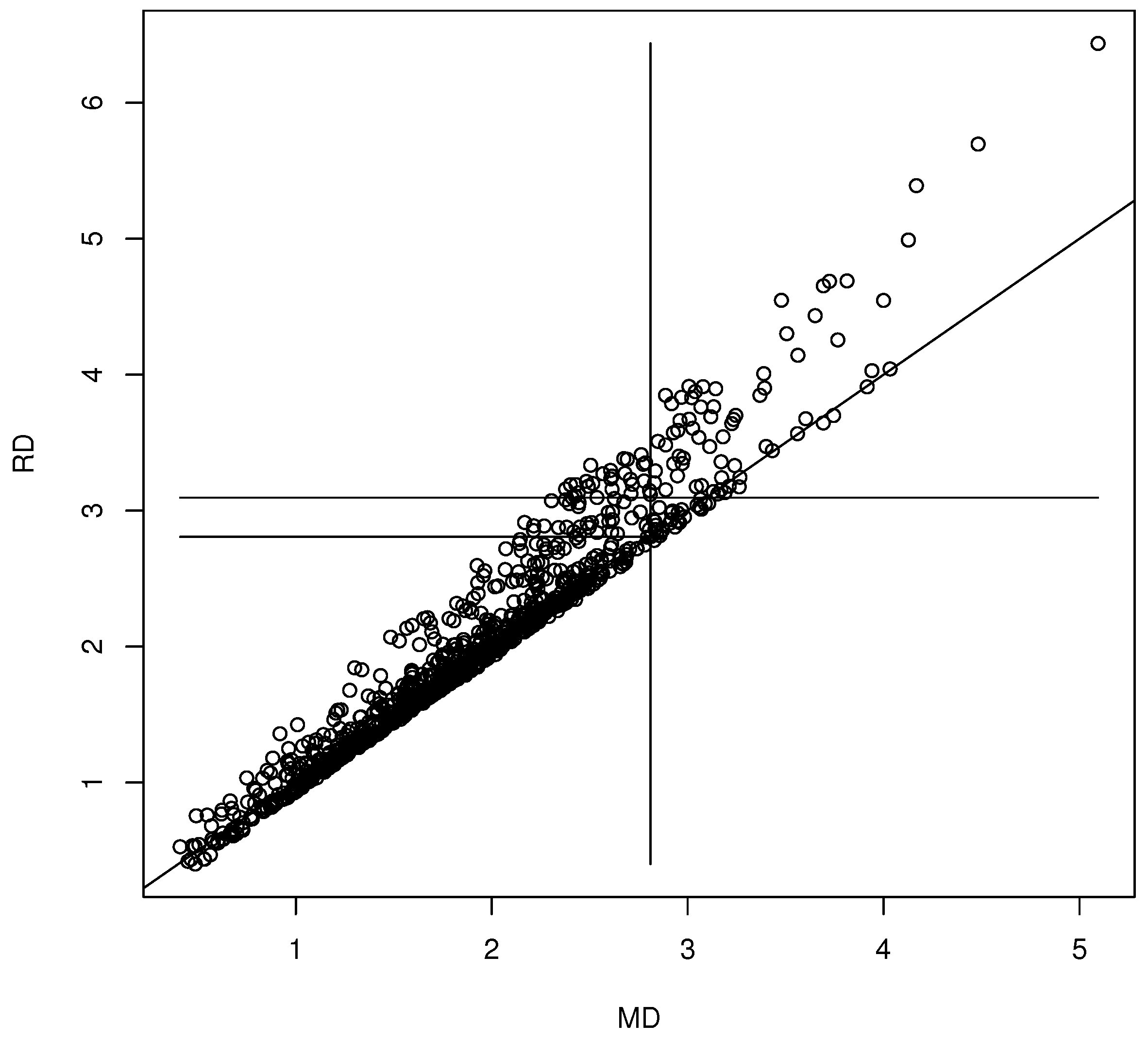
Example 1, in the following section, shows how to use a DD plot to visualize some bootstrap confidence regions. Often, $\sqrt{n}(T_n-\mathit{\theta })\stackrel{D}{\to }{N}_p(\mathbf{0},{\mathbf{\Sigma }}_T)$, $\sqrt{n}(T_i^{*}-T_n)\stackrel{D}{\to }{N}_p(\mathbf{0},{\mathbf{\Sigma }}_T)$, and $\sqrt{n}(T_i^{*}-{\overline{T}}^{*})\stackrel{D}{\to }{N}_p(\mathbf{0},{\mathbf{\Sigma }}_T)$. Then, the plotted points in the DD plot tend to cluster about the identity line in the DD plot. Note that $\{\mathit{w}:D_{\mathit{w}}^2({\overline{T}}^{*},{\mathit{S}}_T^{*})\le D_{\left(U_B\right)}^2\}=\{\mathit{w}:D_{\mathit{w}}({\overline{T}}^{*},{\mathit{S}}_T^{*})\le D_{\left(U_B\right)}\}.$ Hence, $T_i^{*}$ such that $D_{T_i^{*}}({\overline{T}}^{*},{\mathit{S}}_T^{*})\le D_{\left(U_B\right)}$ are in confidence region (10). These $T_i^{*}$ correspond to the points to the left of the vertical line $MD=D_{\left(U_B\right)}$ in the DD plot.

3. Results

Example 1. 

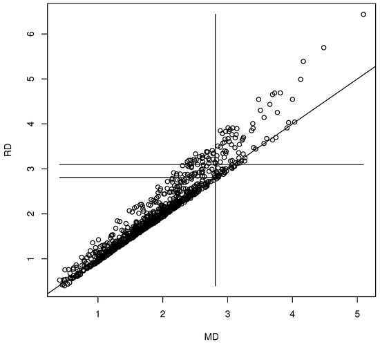
We generated ${\mathit{x}}_i\sim N_4(\mathbf{0},\mathit{I})$ for $i=1,\dots ,250$. The coordinate-wise median was the statistic $T_n$. The nonparametric bootstrap was used with $B=1000$ for the 90% confidence region (10). Then, the $100q_B$th sample quantile of the $D_i$ is the 90.4% quantile. The DD plot of the bootstrap sample is shown in Figure 1. This bootstrap sample was a rather poor sample: the plotted points cluster about the identity line, but for most bootstrap samples, the clustering is tighter (as in Figure 2). The vertical line MD = 2.9098 is the cutoff for the prediction region method 90% confidence region (10). Hence, the points to the left of the vertical line correspond to $T_i^{*}$, which are inside confidence region (10), while the points to the right of the vertical line correspond to $T_i^{*}$, which are outside of confidence region (10). The long horizontal line RD = 3.0995 is the cutoff using the robust estimator. When $\sqrt{n}(T_n-\mathit{\theta })\stackrel{D}{\to }{N}_p(\mathbf{0},{\mathbf{\Sigma }}_T)$, under mild regularity conditions, $\sqrt{n}(T_n-{\overline{T}}_n^{*})\stackrel{P}{\to }\mathit{0}.$ The short horizontal line is RD = 2.8074, and MD = 2.8074 = $\sqrt{{\chi }_{4,0.904}^2}$ is approximately the cutoff $\sqrt{{\chi }_{4,0.9}^2}=2.7892$ that would be used by the standard bootstrap confidence region (mentally drop a vertical line from where the short horizontal line ends at the identity line). Variability in DD plots increases as MD increases.

Figure 1. Visualizing the confidence region with a DD plot.

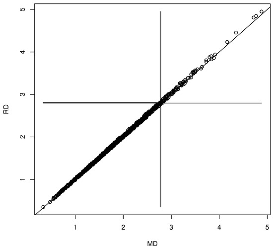
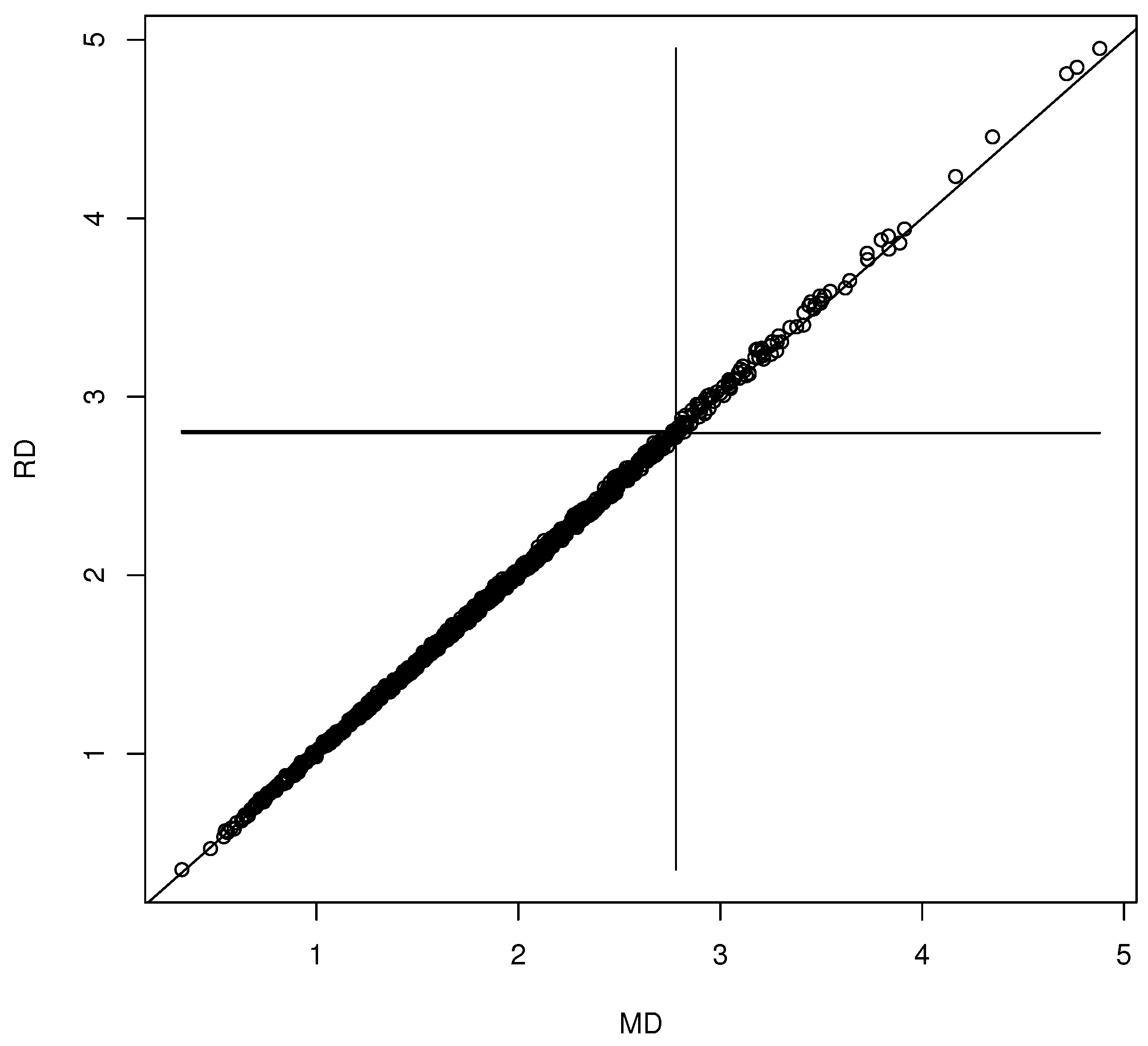
Figure 2. Visualizing the forward selection confidence region for ${\mathit{\beta }}_S$.

Inference after variable selection is an example where the undercoverage of confidence regions can be quite high. See, for example, Kabaila (2009) [23]. Variable selection methods often use the Schwarz (1978) [24] BIC criterion, the Mallows (1973) [25] $C_p$ criterion, or lasso due to Tibshirani (1996) [26]. To describe a variable selection model, we will follow Rathnayake and Olive (2023) [27] closely. Consider regression models where the response variable Y depends on the $p\times 1$ vector of predictor x only through ${\mathit{x}}^T\mathit{\beta }$. Multiple linear regression models, generalized linear models, and proportional hazards regression models are examples of such regression models. Then, a model for variable selection can be described by

$${\mathit{x}}^T\mathit{\beta }={\mathit{x}}_S^T{\mathit{\beta }}_S+{\mathit{x}}_E^T{\mathit{\beta }}_E={\mathit{x}}_S^T{\mathit{\beta }}_S$$

(20)

where $\mathit{x}={({\mathit{x}}_S^T,{\mathit{x}}_E^T)}^T$ is a $p\times 1$ vector of predictors, ${\mathit{x}}_S$ is an $a_S\times 1$ vector, and ${\mathit{x}}_E$ is a $(p-a_S)\times 1$ vector. Given that ${\mathit{x}}_S$ is in the model, ${\mathit{\beta }}_E=0$, and E denotes the subset of terms that can be eliminated given that the subset S is in the model. Since S is unknown, candidate subsets will be examined. Let ${\mathit{x}}_I$ be the vector of a terms from a candidate subset indexed by I, and let ${\mathit{x}}_O$ be the vector of the remaining predictors (out of the candidate submodel). Then,

$${\mathit{x}}^T\mathit{\beta }={\mathit{x}}_I^T{\mathit{\beta }}_I+{\mathit{x}}_O^T{\mathit{\beta }}_O.$$

Suppose that S is a subset of I and that model (20) holds. Then,

$${\mathit{x}}^T\mathit{\beta }={\mathit{x}}_S^T{\mathit{\beta }}_S={\mathit{x}}_S^T{\mathit{\beta }}_S+{\mathit{x}}_{I/S}^T{\mathit{\beta }}_{(I/S)}+{\mathit{x}}_O^{T}0={\mathit{x}}_I^T{\mathit{\beta }}_I$$

where ${\mathit{x}}_{I/S}$ denotes the predictors in I that are not in $S.$ Underfitting occurs if submodel I does not contain S.

To clarify the notation, suppose that $p=4$, a constant $x_1=1$ corresponding to ${\beta }_1$, is always in the model, and $\mathit{\beta }={({\beta }_1,{\beta }_2,0,0)}^T$. Then, there are $J=2^{p-1}=8$ possible subsets of $\{1,2,\dots ,p\}$ that contain 1, including $I_1=\left\{1\right\}$ and $S=I_2=\{1,2\}$. There are $2^{p-a_S}=4$ subsets such that $S\subseteq I_j$. Let ${\widehat{\mathit{\beta }}}_{I_2}={({\widehat{\beta }}_1,{\widehat{\beta }}_2)}^T$ and $x_{I_2}={(x_1,x_2)}^T.$ The full model uses ${\mathit{\beta }}_F=\mathit{\beta }.$

Let $I_{min}$ correspond to the set of predictors selected by a variable selection method such as forward selection or lasso variable selection. If ${\widehat{\mathit{\beta }}}_I$ is $a\times 1$, use zero padding to form the $p\times 1$ vector ${\widehat{\mathit{\beta }}}_{I,0}$ from ${\widehat{\mathit{\beta }}}_I$ by adding 0s corresponding to the omitted variables. For example, if $p=4$ and ${\widehat{\mathit{\beta }}}_{I_{min}}={({\widehat{\beta }}_1,{\widehat{\beta }}_3)}^T$, then the observed variable selection estimator ${\widehat{\mathit{\beta }}}_{VS}={\widehat{\mathit{\beta }}}_{I_{min},0}={({\widehat{\beta }}_1,0,{\widehat{\beta }}_3,0)}^T.$ As a statistic, ${\widehat{\mathit{\beta }}}_{VS}={\widehat{\mathit{\beta }}}_{I_k,0}$ with probabilities ${\pi }_{kn}=P(I_{min}=I_k)$ for $k=1,\dots ,J$, where there are J subsets, e.g., $J=2^p-1$. Then, the variable selection estimator ${\widehat{\mathit{\beta }}}_{VS}={\widehat{\mathit{\beta }}}_{I_{min},0}$, and ${\widehat{\mathit{\beta }}}_{VS}={\widehat{\mathit{\beta }}}_{I_k,0}$ with probabilities ${\pi }_{kn}=P(I_{min}=I_k)$ for $k=1,\dots ,J$, where there are J subsets.

Assume p is fixed. Suppose model (20) holds, and that if $S\subseteq I_j$, where the dimension of $I_j$ is $a_j$, then $\sqrt{n}({\widehat{\mathit{\beta }}}_{I_j}-{\mathit{\beta }}_{I_j})\stackrel{D}{\to }{N}_{a_j}(\mathbf{0},{\mathit{V}}_j)$, where ${\mathit{V}}_j$ is the covariance matrix of the asymptotic multivariate normal distribution. Then,

$$\sqrt{n}({\widehat{\mathit{\beta }}}_{I_j,0}-\mathit{\beta })\stackrel{D}{\to }{N}_p(\mathbf{0},{\mathit{V}}_{j,0})$$

(21)

where ${\mathit{V}}_{j,0}$ adds columns and rows of zeros corresponding to the $x_i$ not in $I_j$, and ${\mathit{V}}_{j,0}$ is singular unless $I_j$ corresponds to the full model. This large-sample theory holds for many models.

If $A_1,A_2,\dots ,A_k$ are pairwise disjoint and if ${\cup }_{i=1}^k{A}_i=S,$ then the collection of sets $A_1,A_2,\dots ,A_k$ is a partition of $S.$ Then, the Law of Total Probability states that if $A_1,A_2,\dots ,A_k$ form a partition of S such that $P\left(A_i\right)>0$ for $i=1,\dots ,k$, then

$$P\left(B\right)=\sum _{j=1}^{k}P(B\cap A_j)=\sum _{j=1}^{k}P\left(B\right|A_j)P\left(A_j\right).$$

Let sets $A_{k+1},\dots ,A_m$ satisfy $P\left(A_i\right)=0$ for $i=k+1,\dots ,m.$ Define $P\left(B\right|A_j)=0$ if $P\left(A_j\right)=0$. Then, a Generalized Law of Total Probability is

$$P\left(B\right)=\sum _{j=1}^{m}P(B\cap A_j)=\sum _{j=1}^{m}P\left(B\right|A_j)P\left(A_j\right).$$

Pötscher (1991) [28] used the conditional distribution of ${\widehat{\mathit{\beta }}}_{VS}|({\widehat{\mathit{\beta }}}_{VS}={\widehat{\mathit{\beta }}}_{I_k,0})$ to find the distribution of ${\mathit{w}}_n=\sqrt{n}({\widehat{\mathit{\beta }}}_{VS}-\mathit{\beta }).$ Let ${\widehat{\mathit{\beta }}}_{I_k,0}^{\mathit{C}}$ be a random vector from the conditional distribution ${\widehat{\mathit{\beta }}}_{I_k,0}|({\widehat{\mathit{\beta }}}_{VS}={\widehat{\mathit{\beta }}}_{I_k,0})$. Let ${\mathit{w}}_{kn}=\sqrt{n}({\widehat{\mathit{\beta }}}_{I_k,0}-\mathit{\beta })|({\widehat{\mathit{\beta }}}_{VS}={\widehat{\mathit{\beta }}}_{I_k,0})\sim \sqrt{n}({\widehat{\mathit{\beta }}}_{I_k,0}^{\mathit{C}}-\mathit{\beta }).$ Denote $F_{\mathit{z}}\left(\mathit{t}\right)=P(z_1\le t_1,\dots ,z_p\le t_p)$ by $P(\mathit{z}\le \mathit{t}).$ Then, Pötscher (1991) [28] used the Generalized Law of Total Probability to prove that the cumulative distribution function (cdf) of $w_n$ is

$$F_{{\mathit{w}}_n}\left(\mathit{t}\right)=P[n^{1/2}({\widehat{\mathit{\beta }}}_{VS}-\mathit{\beta })\le \mathit{t}]=\sum _{k=1}^J{F}_{{\mathit{w}}_{kn}}\left(\mathit{t}\right){\pi }_{kn}.$$

Hence, ${\widehat{\mathit{\beta }}}_{VS}$ has a mixture distribution of the ${\widehat{\mathit{\beta }}}_{I_k,0}^C$ with probabilities ${\pi }_{kn}$, and ${\mathit{w}}_n$ has a mixture distribution of the ${\mathit{w}}_{kn}$ with probabilities ${\pi }_{kn}.$

For the following Rathnayake and Olive (2023) [27] theorem, the first assumption is $P(S\subseteq I_{min})\to 1$ as $n\to \infty$. Then, the variable selection estimator corresponding to $I_{min}$ underfits with probability going to zero, and the assumption holds under regularity conditions, if BIC and AIC is used for many parametric regression models such as GLMs. See Charkhi and Claeskens (2018) [29] and Claeskens and Hjort (2008, pp. 70, 101, 102, 114, 232) [30]. This assumption is a necessary condition for a variable selection estimator to be a consistent estimator. See Zhao and Yu (2006) [31]. Thus, if a sparse estimator that performs variable selection is a consistent estimator of $\mathit{\beta }$, then $P(S\subseteq I_{min})\to 1$ as $n\to \infty$. Hence, Theorem 2 proves that the lasso variable selection estimator is a $\sqrt{n}$ consistent estimator of $\mathit{\beta }$ if lasso is consistent. Charkhi and Claeskens (2018) [29] showed that ${\mathit{w}}_{jn}=\sqrt{n}({\widehat{\mathit{\beta }}}_{I_j,0}^C-\mathit{\beta })\stackrel{D}{\to }{\mathit{w}}_j$ if $S\subseteq I_j$ for the maximum likelihood estimator with AIC, and gave a forward selection example. For a multiple linear regression model where S is the model with exactly one predictor that can be deleted, then only ${\pi }_S$ and ${\pi }_F$ are positive. If the $C_p$ criterion is used, then it can be shown that ${\pi }_S=P({\chi }_1^2<2)=0.8427$, and ${\pi }_F=1-{\pi }_S=0.1573$. Theorem 2 proves that w is a mixture distribution of the ${\mathit{w}}_j$ with probabilities ${\pi }_j$.

Theorem 2. 

Assume $P(S\subseteq I_{min})\to 1$ as $n\to \infty$, and let ${\widehat{\mathit{\beta }}}_{VS}={\widehat{\mathit{\beta }}}_{I_k,0}$ with probabilities ${\pi }_{kn}$, where ${\pi }_{kn}\to {\pi }_k$ as $n\to \infty$. Denote the positive ${\pi }_k$ by ${\pi }_j$. Assume

${\mathit{w}}_{jn}=\sqrt{n}({\widehat{\mathit{\beta }}}_{I_j,0}^{\mathit{C}}-\mathit{\beta })\stackrel{D}{\to }{\mathit{w}}_j$. Then,

$${\mathit{w}}_n=\sqrt{n}({\widehat{\mathit{\beta }}}_{VS}-\mathit{\beta })\stackrel{D}{\to }\mathit{w}$$

(22)

where the cdf of w is $F_{\mathit{w}}\left(\mathit{t}\right)={\sum }_j{\pi }_j{F}_{{\mathit{w}}_j}\left(\mathit{t}\right)$.

Rathnayake and Olive (2023) [27] suggested the following bootstrap procedure. Use a bootstrap method for the full model, such as the nonparametric bootstrap or the residual bootstrap, and then compute the full model and the variable selection estimator from the bootstrap data set. Repeat this B times to obtain the bootstrap sample for the full model and for the variable selection model. They could only prove that the bootstrap procedure works under very strong regularity conditions such as a ${\pi }_i=1$ in Theorem 2, where ${\pi }_S=1$ is known as the oracle property. See Claeskens and Hjort (2008, pp. 101–114) [30] for references for the oracle property. For many statistics, a bootstrap data cloud $T_1^{*},\dots ,T_B^{*}$ and a data cloud from B iid statistics $T_1,\dots ,T_B$ tend to have similar variability. Rathnayake and Olive (2023) [27] suggested that when T is the variable selection estimator ${\widehat{\mathit{\beta }}}_{VS}$, the bootstrap data cloud often has more variability than the iid data cloud, and that this result tends to increase the bootstrap confidence region coverage.

For variable selection with the $p\times 1$ vector ${\widehat{\mathit{\beta }}}_{I_{min},0}$, consider testing $H_0:\mathit{A}\mathit{\beta }={\mathit{\theta }}_0$ versus $H_1:\mathit{A}\mathit{\beta }\ne {\mathit{\theta }}_0$ with $\mathit{\theta }=\mathit{A}\mathit{\beta }$, where oftentimes, ${\mathit{\theta }}_0=0$. Then, let $T_n=\mathit{A}{\widehat{\mathit{\beta }}}_{I_{min},0}$ and let $T_i^{*}=\mathit{A}{\widehat{\mathit{\beta }}}_{I_{min},0,i}^{*}$ for $i=1,\dots ,B$. The shorth estimator can be applied to a bootstrap sample ${\widehat{\beta }}_{i1}^{*},\dots ,{\widehat{\beta }}_{iB}^{*}$ to obtain a confidence interval for ${\beta }_i$. Here, $T_n={\widehat{\beta }}_i$ and $\theta ={\beta }_i$. The simulations used $\theta =\mathit{A}\mathit{\beta }={\beta }_i$, $\mathit{\theta }=\mathit{A}\mathit{\beta }={\mathit{\beta }}_S=\mathbf{1}$, and $\mathit{\theta }=\mathit{A}\mathit{\beta }={\mathit{\beta }}_E=\mathbf{0}$. Let the multiple linear regression model $Y_i=1+1x_{i,2}+\dots +1x_{i,k+1}+e_i$ for $i=1,\dots ,n$. Hence, $\mathit{\beta }={(1,\dots ,1,0,\dots ,0)}^T$ with $k+1$ ones and $p-k-1$ zeros.

The regression models used the residual bootstrap with the forward selection estimator ${\widehat{\mathit{\beta }}}_{I_{min},0}$. Table 1 gives results for when the iid errors $e_i\sim N(0,1)$ with $n=100$, $p=4$, and $k=1$. Table 1 shows two rows for each model giving the observed confidence interval coverages and average lengths of the confidence intervals. The nominal coverage was 95%. The term “reg" is for the full model regression, and the term “vs" is for forward selection. The last six columns give results for the tests. The terms pr, hyb, and br are for prediction region method (10), hybrid region (12), and Bickel and Ren region (11). The 0 indicates that the test was $H_0:{\mathit{\beta }}_E={({\beta }_3,{\beta }_4)}^T=\mathbf{0}$ versus $H_1:{\mathit{\beta }}_E\ne \mathbf{0}$, while the 1 indicates that the test was $H_0:{\mathit{\beta }}_S={({\beta }_1,{\beta }_2)}^T=\mathbf{1}$ versus $H_1:{\mathit{\beta }}_S\ne \mathbf{1}$. The length and coverage = P (fail to reject $H_0$) for the interval $[0,D_{\left(U_B\right)}]$ or $[0,D_{(U_B,T)}]$, where $D_{\left(U_B\right)}$ or $D_{(U_B,T)}$ is the cutoff for the confidence region. The cutoff will often be near $\sqrt{{\chi }_{g,0.95}^2}$ if the statistic T is asymptotically normal. Note that $\sqrt{{\chi }_{2,0.95}^2}=2.448$ is close to 2.45 for the full model regression bootstrap tests. For the full model, $\sqrt{n}$ len $\to 3.92$ as $n\to \infty$ for the simulated data, and the shorth 95% confidence intervals have simulated length $\approx 0.398\approx 3.92/10=0.392.$ The variable selection estimator and the full model estimator were similar for ${\beta }_1,{\beta }_2$, and ${\mathit{\beta }}_S$. The two estimators differed for ${\beta }_3,{\beta }_4,$ and ${\mathit{\beta }}_E$ because ${\widehat{\beta }}_i^{*}=0$ often occurred for $i=3$ and 4. In particular, the confidence interval coverages for the variable selection estimator were very high, but the average lengths were shorter than those for the full model. If $x_3$ was never selected, then ${\widehat{\beta }}_3^{*}\equiv 0$ for all runs, and the confidence interval would be [0, 0] with 100% coverage and zero length.

Table 1. Bootstrapping OLS forward selection with $C_p$, $e_i\sim N(0,1)$.

	${\mathit{\beta }}_1$	${\mathit{\beta }}_2$	${\mathit{\beta }}_{\mathit{p}-1}$	${\mathit{\beta }}_{\mathit{p}}$	pr0	hyb0	br0	pr1	hyb1	br1
reg	0.946	0.950	0.947	0.948	0.940	0.941	0.941	0.937	0.936	0.937
len	0.396	0.399	0.399	0.398	2.451	2.451	2.452	2.450	2.450	2.451
vs	0.948	0.950	0.997	0.996	0.991	0.979	0.991	0.938	0.939	0.940
len	0.395	0.398	0.323	0.323	2.699	2.699	3.002	2.450	2.450	2.457

Note that for the variable selection estimator with $H_0:{\mathit{\beta }}_E=\mathbf{0}$, the average cutoff values were near 2.7 and 3.0, which are larger than the ${\chi }_2^2$ cutoff 2.448. Hence, using the standard bootstrap confidence region (16) would result in undercoverage. For $H_0:{\mathit{\beta }}_S=\mathbf{1}$, the bootstrap estimator often appeared to be approximately multivariate normal. Example 2 illustrates this result with a DD plot.

Example 2. 

We generated ${\mathit{x}}_i\sim N_4(\mathbf{0},\mathit{I})$ and $Y_i=1+x_{i1}+x_{i2}+x_{i3}+e_i$ for $i=1,\dots ,n=1000$ with the $e_i$ iid $N(0,1)$ and $\mathit{\beta }={\mathit{\beta }}_F={(1,1,1,1,0)}^T$. Then, we examined several bootstrap methods for multiple linear regression variable selection. The nonparametric bootstrap draws n cases ${({\mathit{x}}_j^T,Y_j)}^T$ with replacement from the n original cases, and then selects variables on the resulting data set, resulting in ${\widehat{\mathit{\beta }}}_I^{*}$. If ${\widehat{\mathit{\beta }}}_I^{*}$ is $a\times 1$, use zero padding to form the $p=5\times 1$ vector ${\widehat{\mathit{\beta }}}_{I,0}^{*}={\widehat{\mathit{\beta }}}_1^{*}$ from ${\widehat{\mathit{\beta }}}_I$ by adding 0s corresponding to the omitted variables. Repeat $B=1000$ times to obtain the bootstrap sample ${\widehat{\mathit{\beta }}}_1^{*},\dots ,{\widehat{\mathit{\beta }}}_B^{*}$. Typically, the full model $I=F$ or the submodel $I=S$ that omitted $x_{i4}$ was selected. The residual bootstrap using the full model residuals was also used, where $Y_i^{*}=\left(1{\mathit{x}}_i^T\right)\widehat{\mathit{\beta }}+r_i^{*}$ for $i=1,\dots ,n$ where the $r_i^{*}$ are sampled with replacement from the full model residuals $r_1,\dots ,r_n$. Forward selection and backward elimination could be used with the $C_p$ or BIC criterion, or lasso could be used to perform the variable selection. Let ${\widehat{\mathit{\beta }}}_{S:I,0}^{*}$ be obtained from ${\widehat{\mathit{\beta }}}_{I,0}^{*}$ by leaving out the fifth value. Hence, if ${\widehat{\mathit{\beta }}}_{I,0}^{*}={(0.9351,1.0252,0.9251,0.9542,0)}^T,$ then ${\widehat{\mathit{\beta }}}_{S:I,0}^{*}={(0.9351,1.0252,0.9251,0.9542)}^T$. Figure 2 shows the DD plot for the confidence region corresponding to the ${\widehat{\mathit{\beta }}}_{S:I,0}^{*}$ using forward selection with the $C_p$ criterion. This confidence region corresponds to the test $H_0:{\mathit{\beta }}_S=\mathit{b}={(b_1,b_2,b_3,b_4)}^T$, e.g., $\mathit{b}=\mathbf{1}$. Plots created with backward elimination and lasso were similar. Rathnayake and Olive (2023) [27] obtained the large-sample theory for the variable selection estimators ${\widehat{\mathit{\beta }}}_{VS}={\widehat{\mathit{\beta }}}_{I,0}$ for multiple linear regression and many other regression methods. The limiting distribution is a complicated non-normal mixture distribution by Theorem 2, but in simulations, where S is known, the ${\widehat{\mathit{\beta }}}_{S:I,0}^{*}$ often appeared to have an approximate multivariate normal distribution.

A small simulation study was conducted on large-sample 95% confidence regions. The coordinate-wise median was used since this statistic is moderately difficult to bootstrap. We used 5000 runs. Then, the coverage within [0.94, 0.96] suggests that the true coverage is near the nominal coverage 0.95. The simulation used 10 distributions, where xtype = 1 for $N_p(\mathbf{0},\mathit{I});$ xtype = 2, 3, 4, and 5 for $(1-\delta )N_p(\mathit{0},\mathit{I})+\delta N_p(0,25\mathit{I})$; xtype = 6, 7, 8, and 9 for a multivariate $t_d$ with d = 3, 5, 19, or d, given by the user; and xtype=10 for a log-normal distribution shifted to have the coordinate-wise median = 0. If w corresponds to one of the above distributions, then $\mathit{x}=\mathit{A}\mathit{w}$ with $\mathit{A}=diag(\sqrt{1},\sqrt{2},\dots ,\sqrt{p})$. Then, the population coordinate-wise median is 0 for each distribution. Table 2 shows the coverages and average cutoff for four large-sample confidence regions: (10), (19), with $n_V=B=1000$, (19) with $n_V=B=49$, and (19) with $n_V=B=99$. The coverage is the proportion of times that the confidence region contained $\mathit{\theta }=\mathbf{0}$, where $\mathit{\theta }$ is a $p\times 1$ vector. Each confidence region has a cutoff, $D=\sqrt{D^2}$, that depends on the bootstrap sample, and the average of the 5000 cutoffs is given. Here, $D^2=D_{\left(U_B\right)}^2$ for confidence region (10), while $D^2=D_{\left(U_V\right)}^2$ for confidence region (19), where the cutoff also depends on $n_V$. The coverages were usually between 0.94 and 0.96. The average cutoffs for the prediction region method’s large-sample 95% confidence region tended to be very close to the average cutoffs for confidence region (19) with $n_V=B=1000$. Note that $\sqrt{{\chi }_{2,0.95}^2}=2.4477$ and $\sqrt{{\chi }_{4,0.95}^2}=3.0802$ are the cutoffs for the standard bootstrap confidence region (15). The ratio of volumes of the two confidence regions is volume (10)/volume (19) ${\displaystyle ={(D_{\left(U_B\right)}/D_{\left(U_V\right)})}^p}$.

Table 2. Coverages and average cutoffs for some large-sample 95% confidence regions, B = 1000.

n	p	Dist	CR (10)	(19), ${\mathit{n}}_{\mathit{V}}=1000$	(19), ${\mathit{n}}_{\mathit{V}}=49$	(19), ${\mathit{n}}_{\mathit{V}}=99$
100	2	N	(0.9430,2.4931)	(0.9450,2.5015)	(0.9536,2.7127)	(0.9452,2.5351)
100	2	LN	(0.9494,2.5025)	(0.9488,2.5088)	(0.9598,2.7401)	(0.9500,2.5539)
100	4	N	(0.9386,3.1738)	(0.9384,3.1795)	(0.9522,3.3922)	(0.9384,3.2177)
100	4	LN	(0.9456,3.2012)	(0.9466,3.2046)	(0.9598,3.4512)	(0.9468,3.2543)
200	4	N	(0.9476,3.1489)	(0.9480,3.1575)	(0.9590,3.3510)	(0.9490,3.1948)
200	4	LN	(0.9432,3.1673)	(0.9440,3.1700)	(0.9554,3.3861)	(0.9440,3.2065)

4. Discussion

The bootstrap was due to Efron (1979) [32]. Also, see Efron (1982) [3] and Bickel and Freedman (1981) [33]. Ghosh and Polansky (2014) and Politis and Romano (1994) [34,35] are useful references for bootstrap confidence regions. For a small dimension p, nonparametric density estimation can be used to construct confidence regions and prediction regions. See, for example, Hall (1987) and Hyndman (1986) [36,37] Visualizing a bootstrap confidence region is useful for checking whether the asymptotic normal approximation for the statistic is good since the plotted points will then tend to cluster tightly about the identity line. Making five plots corresponding to five bootstrap samples can be used to check the variability of the plots and the probability of obtaining a bad sample. For Example 1, most of the bootstrap samples produced plots that had tighter clustering about the identity line than the clustering in Figure 1.

The new bootstrap confidence region (19) used the fact that bootstrap confidence region (10) is simultaneously a prediction region for a future bootstrap statistic $T_F^{*}$ and a confidence region for $\mathit{\theta }$ with the same asymptotic coverage $1-\delta$. Hence, increasing the coverage as a prediction region also increases the coverage as a confidence region. The data splitting technique used to increase the coverage only depends on the $T_i^{*}$ being iid with respect to the bootstrap distribution. Correction factor (8) increases the coverage, but this calibration technique needed intensive simulation.

Calibrating a bootstrap confidence region is useful for several reasons. For simulations, computation time can be reduced if B can be reduced. Using correction factor (8) is faster than using the two-sample bootstrap of Section 2.1, but the two-sample bootstrap can be used to check the accuracy of (8), as in Table 2 with $n_V=B$. For a nominal 95% prediction region, correction factor (8) increases the coverage to at most 97.5% of the training data. Coverage for test data ${\mathit{x}}_f$ tends to be worse than coverage for training data. Using the cutoff $D_{\left(U_B\right)}^2$ of (8) gives better coverage than using cutoff $D_{\left(U\right)}^2$ with $U=\lceil B(1-\delta )\rceil$. The two calibration methods in this paper were first applied to prediction regions, and work for bootstrap confidence regions (10) and (11) since those two regions are also prediction regions for $T_f^{*}$.

Plots and simulations were conducted in R. See R Core Team (2020) [38]. Welagedara (2023) [39] lists some R functions for bootstrapping several statistics. The programs used are in the collection of functions slpack.txt. See http://parker.ad.siu.edu/Olive/slpack.txt, accessed on 1 August 2024. The function ddplot4 applied to the bootstrap sample can be used to visualize the bootstrap prediction region method’s confidence region. The function medbootsim was used for Table 2. Some functions for bootstrapping multiple linear regression variable selection with the residual bootstrap are belimboot for backward elimination using $C_p$, bicboot for forward selection using BIC, fselboot for forward selection using $C_p$, lassoboot for lasso variable selection, and vselboot for all of the subsets’ variable selection with $C_p$.

References

- Olive, D.J. Robust Multivariate Analysis; Springer: New York, NY, USA, 2017. [Google Scholar]
- Frey, J. Data-driven nonparametric prediction intervals. J. Stat. Plan. Inference 2013, 143, 1039–1048. [Google Scholar] [CrossRef]
- Efron, B. The Jackknife, the Bootstrap and Other Resampling Plans; SIAM: Philadelphia, PA, USA, 1982. [Google Scholar]
- Hall, P. Theoretical comparisons of bootstrap confidence intervals. Ann. Stat. 1988, 16, 927–985. [Google Scholar] [CrossRef]
- Pelawa Watagoda, L.C.R.; Olive, D.J. Bootstrapping multiple linear regression after variable selection. Stat. Pap. 2021, 62, 681–700. [Google Scholar] [CrossRef]
- Olive, D.J. Asymptotically optimal regression prediction intervals and prediction regions for multivariate data. Int. J. Stat. Probab. 2013, 2, 90–100. [Google Scholar] [CrossRef]
- Olive, D.J. Applications of hyperellipsoidal prediction regions. Stat. Pap. 2018, 59, 913–931. [Google Scholar] [CrossRef]
- Bickel, P.J.; Ren, J.J. The Bootstrap in hypothesis testing. In State of the Art in Probability and Statistics: Festschrift for William R. van Zwet; de Gunst, M., Klaassen, C., van der Vaart, A., Eds.; The Institute of Mathematical Statistics: Hayward, CA, USA, 2001; pp. 91–112. [Google Scholar]
- Rajapaksha, K.W.G.D.H.; Olive, D.J. Wald type tests with the wrong dispersion matrix. Commun. Stat.-Theory Methods 2024, 53, 2236–2251. [Google Scholar] [CrossRef]
- Chew, V. Confidence, prediction and tolerance regions for the multivariate normal distribution. J. Am. Stat. Assoc. 1966, 61, 605–617. [Google Scholar] [CrossRef]
- Efron, B. Estimation and accuracy after model selection. J. Am. Stat. Assoc. 2014, 109, 991–1007. [Google Scholar] [CrossRef] [PubMed]
- Haile, M.G.; Zhang, L.; Olive, D.J. Predicting random walks and a data splitting prediction region. Stats 2024, 7, 23–33. [Google Scholar] [CrossRef]
- Barndorff-Nielsen, O.E.; Cox, D.R. Prediction and asymptotics. Bernoulli 1996, 2, 319–340. [Google Scholar] [CrossRef]
- Beran, R. Calibrating prediction regions. J. Am. Stat. Assoc. 1990, 85, 715–723. [Google Scholar] [CrossRef]
- Fonseca, G.; Giummole, F.; Vidoni, P. A note about calibrated prediction regions and distributions. J. Stat. Plan. Inference 2012, 142, 2726–2734. [Google Scholar] [CrossRef]
- Hall, P.; Peng, L.; Tajvidi, N. On prediction intervals based on predictive likelihood or bootstrap methods. Biometrika 1999, 86, 871–880. [Google Scholar] [CrossRef]
- Hall, P.; Rieck, A. Improving coverage accuracy of nonparametric prediction intervals. J. R. Stat. Soc. B 2001, 63, 717–725. [Google Scholar] [CrossRef]
- Ueki, M.; Fueda, K. Adjusting estimative prediction limits. Biometrika 1996, 94, 509–511. [Google Scholar] [CrossRef]
- DiCiccio, T.J.; Efron, B. Bootstrap confidence intervals. Stat. Sci. 1996, 11, 189–228. [Google Scholar] [CrossRef]
- Loh, W.Y. Calibrating confidence coefficients. J. Am. Stat. Assoc. 1987, 82, 155–162. [Google Scholar] [CrossRef]
- Loh, W.Y. Bootstrap calibration for confidence interval construction and selection. Stat. Sin. 1991, 1, 477–491. [Google Scholar]
- Rousseeuw, P.J.; Van Driessen, K. A fast algorithm for the minimum covariance determinant estimator. Technometrics 1999, 41, 212–223. [Google Scholar] [CrossRef]
- Kabaila, P. The coverage properties of confidence regions after model selection. Int. Stat. Rev. 2009, 77, 405–414. [Google Scholar] [CrossRef]
- Schwarz, G. Estimating the dimension of a model. Ann. Stat. 1978, 6, 461–464. [Google Scholar] [CrossRef]
- Mallows, C. Some comments on Cp. Technometrics 1973, 15, 661–676. [Google Scholar]
- Tibshirani, R. Regression shrinkage and selection via the lasso. J. R. Stat. Soc. B 1996, 58, 267–288. [Google Scholar] [CrossRef]
- Rathnayake, R.C.; Olive, D.J. Bootstrapping some GLMs and survival regression models after variable selection. Commun. Stat.-Theory Methods 2023, 52, 2625–2645. [Google Scholar] [CrossRef]
- Pötscher, B. Effects of model selection on inference. Econom. Theory 1991, 7, 163–185. [Google Scholar] [CrossRef]
- Charkhi, A.; Claeskens, G. Asymptotic post-selection inference for the Akaike information criterion. Biometrika 2018, 105, 645–664. [Google Scholar] [CrossRef]
- Claeskens, G.; Hjort, N.L. Model Selection and Model Averaging; Cambridge University Press: New York, NY, USA, 2008. [Google Scholar]
- Zhao, P.; Yu, B. On model selection consistency of lasso. J. Mach. Learn. Res. 2006, 7, 2541–2563. [Google Scholar]
- Efron, B. Bootstrap methods, another look at the jackknife. Ann. Stat. 1979, 7, 1–26. [Google Scholar] [CrossRef]
- Bickel, P.J.; Freedman, D.A. Some asymptotic theory for the bootstrap. Ann. Stat. 1981, 9, 1196–1217. [Google Scholar] [CrossRef]
- Ghosh, S.; Polansky, A.M. Smoothed and iterated bootstrap confidence regions for parameter vectors. J. Mult. Anal. 2014, 132, 171–182. [Google Scholar] [CrossRef]
- Politis, D.N.; Romano, J.P. Large sample confidence regions based on subsamples under minimal assumptions. Ann. Stat. 1994, 22, 2031–2050. [Google Scholar] [CrossRef]
- Hall, P. On the bootstrap and likelihood-based confidence regions. Biometrika 1987, 74, 481–493. [Google Scholar] [CrossRef]
- Hyndman, R.J. Computing and graphing highest density regions. Am. Stat. 1996, 50, 120–126. [Google Scholar] [CrossRef]
- R Core Team. R: A Language and Environment for Statistical Computing; R Foundation for Statistical Computing: Vienna, Austria, 2020; Available online: www.r-project.org (accessed on 1 August 2024).
- Welagedara, W.A.D.M. Model Selection, Data Splitting for ARMA Time Series, and Visualizing Some Bootstrap Confidence Regions. Ph.D. Thesis, Southern Illinois University, Carbondale, IL, USA, 2023. Available online: http://parker.ad.siu.edu/Olive/swelagedara.pdf (accessed on 1 August 2024).
Disclaimer/Publisher’s Note: The statements, opinions and data contained in all publications are solely those of the individual author(s) and contributor(s) and not of MDPI and/or the editor(s). MDPI and/or the editor(s) disclaim responsibility for any injury to people or property resulting from any ideas, methods, instructions or products referred to in the content. |
© 2024 by the authors. Licensee MDPI, Basel, Switzerland. This article is an open access article distributed under the terms and conditions of the Creative Commons Attribution (CC BY) license (https://creativecommons.org/licenses/by/4.0/).