
Unsupervised Feature Selection with Latent Relationship Penalty Term


Abstract
:1. Introduction
- A novel unsupervised feature selection with latent relationship penalty term is presented, which simultaneously performs an improved latent representation learning on the attribute scores of the subspace matrix and imposes a sparse term on the feature transformation matrix.
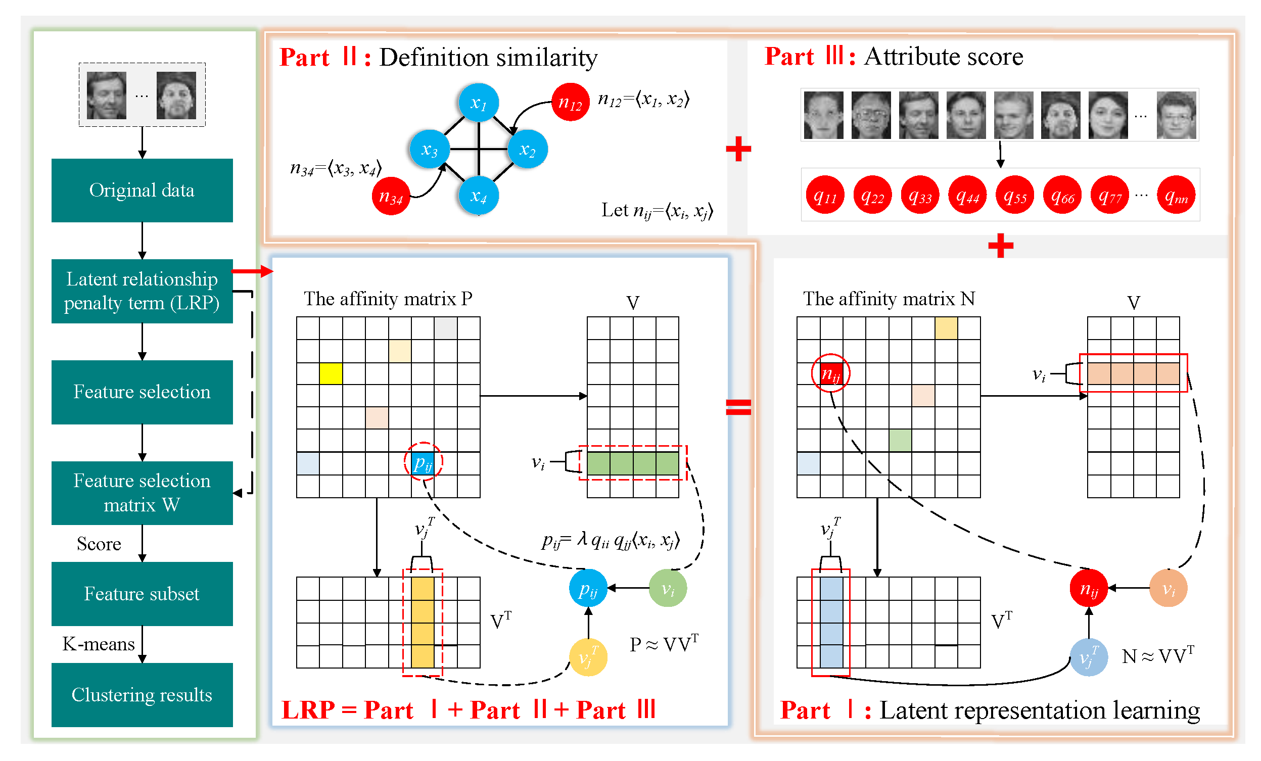
- The latent relationship penalty term, an improved latent representation learning, is proposed. By constructing a novel affinity measurement strategy based on pairwise relationships and attribute scores of samples, this penalty term can exploit the uniqueness of samples to reduce interference from noise and ensure that the spatial structure of both the original data and the subspace data remains consistent, which is different from other existing models.
- An optimum algorithm with convergence is designed and extensive experiments are conducted: (1) LRPFS has shown superior performance on publicly available datasets compared to other existing models in terms of clustering performance and more remarkable capability of discriminative feature selection. (2) Experiments verify that LRPFS has fast convergence, short computation time, and significant performance by explicitly evaluating an attribute score for each individual to eliminate redundant features.
2. Related Works
2.1. Notations
2.2. Review of Feature Selection and Latent Representation Learning
2.3. Inner Product Space
3. Methodology
3.1. Latent Relationship Penalty Term
3.1.1. Preservation of Data Structures
3.1.2. Exploring the Uniqueness of Individuals
3.2. Objective Function
3.3. Optimization
- (1)
- Fix and update :
- (2)
- Fix and update :
| Algorithm 1: LRPFS algorithm steps |
| 1: Input: Data matrix ; Parameters , , , and ; The maximum number of iterations ; |
| 2: Initialization: The iteration time ; ; ; ; Construct the attribute score matrix ; |
| 3: while not converged do 4: Update using ; 5: Update using ; 6: Update using ; 7: Update by: ; 8: end while |
| 9: Output: The feature transformation matrix and the subspace matrix . |
| 10: Feature selection: Calculate the scores of the features according to and select the first features with high scores. |
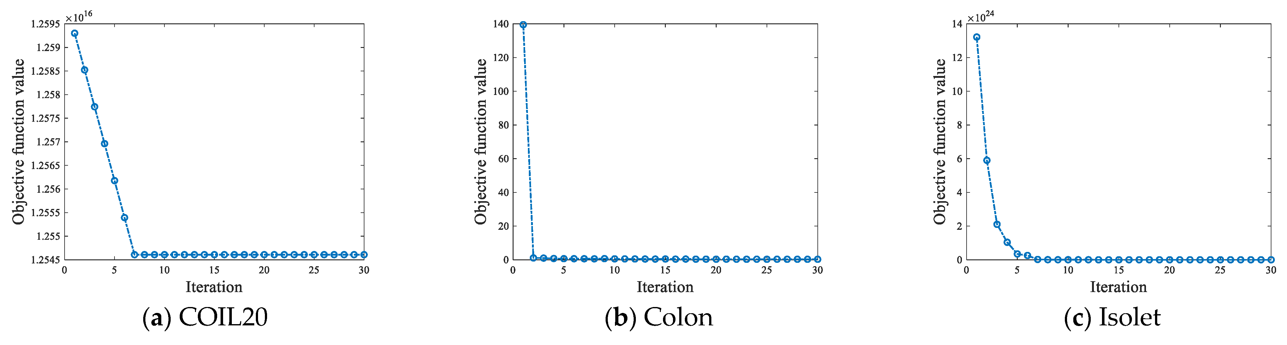
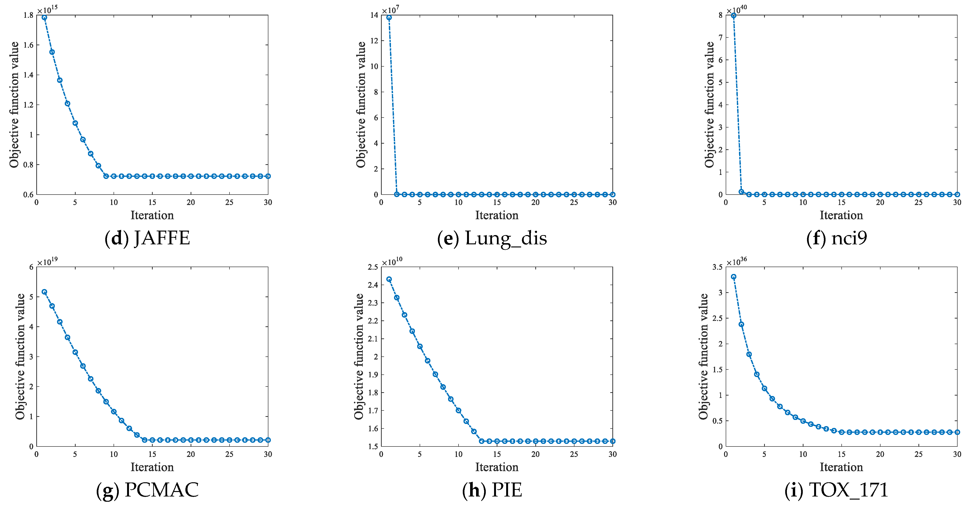
3.4. Convergence Analysis
3.5. Computational Time Complexity
4. Experiments
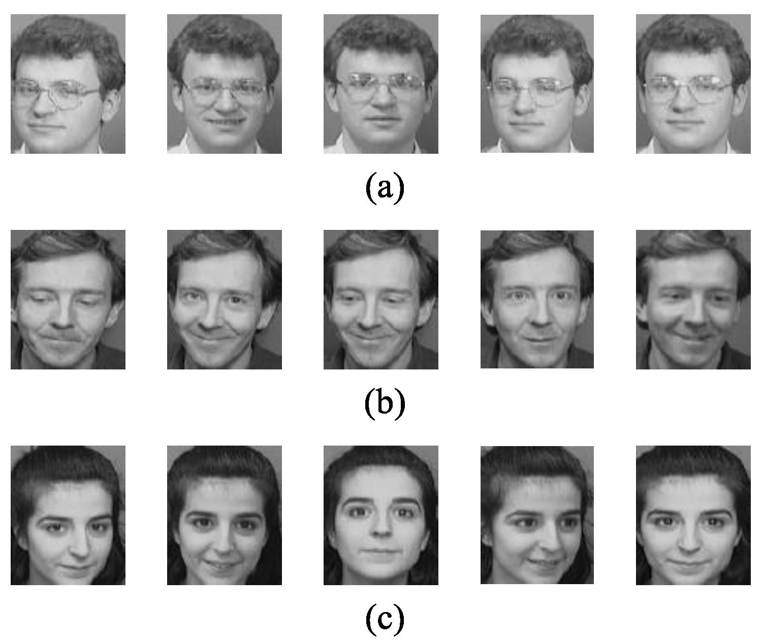
4.1. Datasets
4.2. Comparison Methods
4.3. Evaluation Metrics
4.4. Experimental Settings
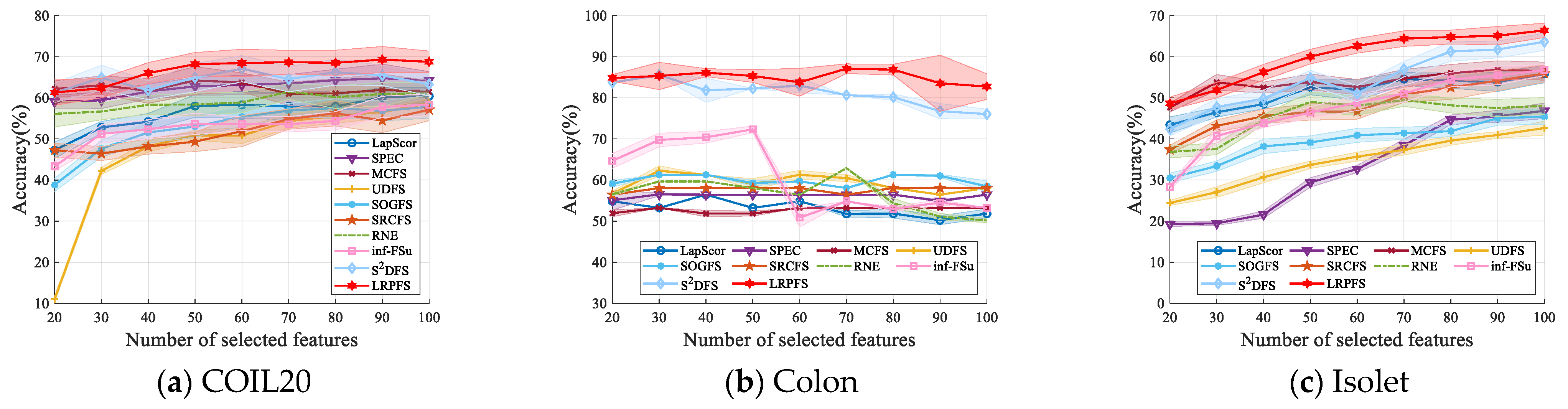
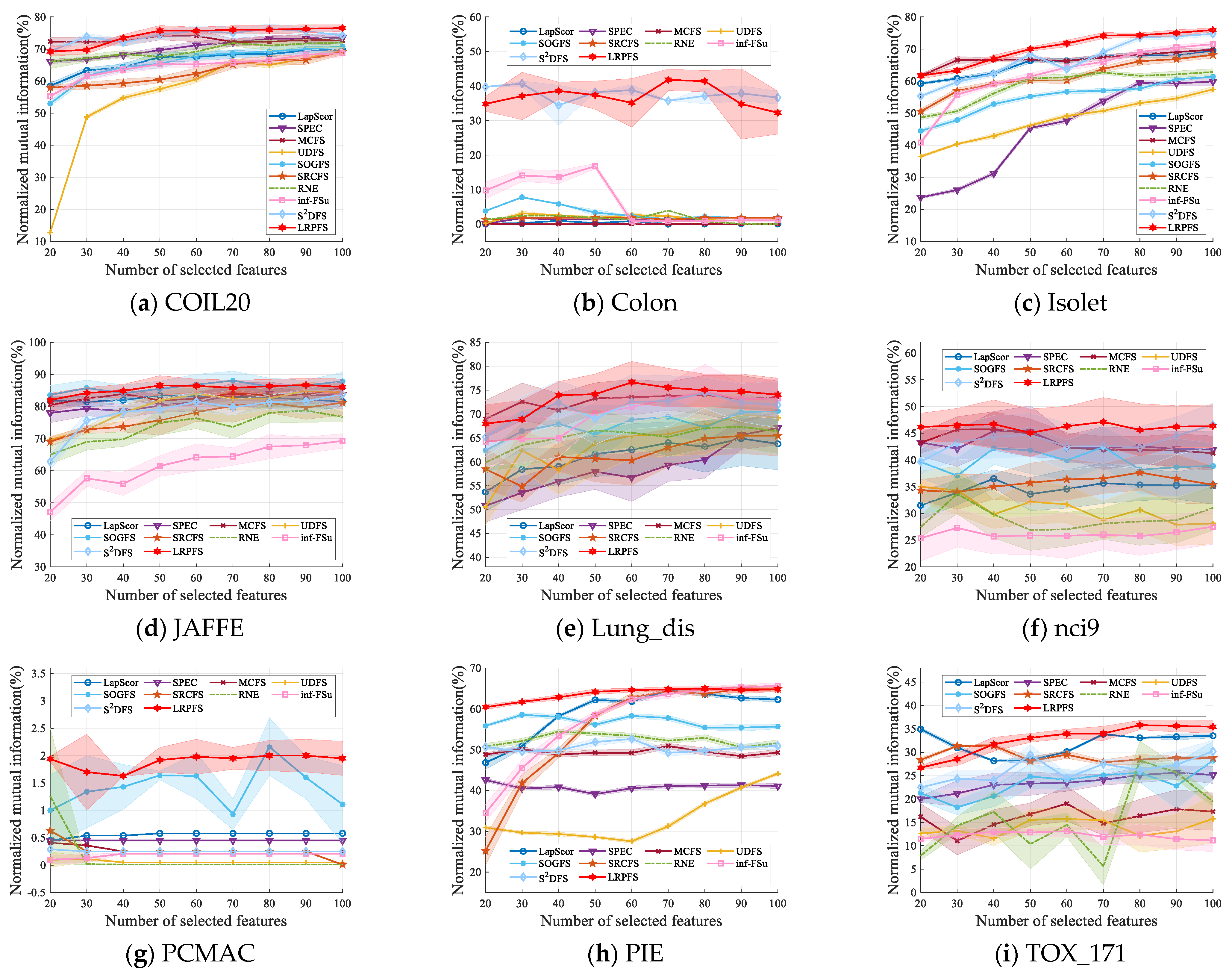
4.5. Comparison Experiment
- (1)
- Overall, most of the UFS methods outperform baseline across a majority of datasets. This performance differential highlights the substantial superiority of these UFS methods in effectively eliminating irrelevant and redundant features.
- (2)
- The results presented in Table 2 and Table 3 indicate that our proposed method, LRPFS, achieves significant performance compared to other state-of-the-art techniques. Specially, LRPFS showcases a substantial increase in Accuracy (ACC) of 32.26%, 30.65%, 30.57%, 33.87%, 24.84%, 25.81%, 29.04%, 24.2%, 14.76%, and 1.54%, respectively, as compared to baseline, LapScor, SPEC, MCFS, UDFS, SOGFS, SRCFS, RNE, inf-FSU, and S2DFS. The main reason for this phenomenon is that LRPFS excels in extracting the inherent information within the data structure and assigning unique attribute scores to individual samples. These distinct attributes significantly contribute to its outstanding performance, especially on the Colon dataset.
- (3)
- The insights revealed by the results in Table 4 serve to emphasize LRPFS’s remarkable competitiveness in terms of computation time against a significant proportion of the algorithms under comparison. While the performance of LRPFS might be slightly inferior to baseline, LapScor, and MCFS, it still exhibits excellent computational efficiency, coupled with the highest clustering accuracy. This is particularly evident when comparing LRPFS with UDFS, SOGFS, RNE, inf-FSU, and S2DFS. Compared with baseline, the running time of LRPFS on some datasets with few samples, such as Colon, nci9, and TOX_171, is slower than baseline. The main reason is that the process of selecting discriminant features takes a certain amount of time. However, when dealing with datasets with large samples such as PIE and Isolet, the running time of LRPFS is superior to baseline and the clustering accuracy is also significantly improved, which verifies the dimension reduction capability of LRPFS and provides a theoretical basis for the implementation of practical problems.
- (4)
- MCFS performs better than SPEC on Isolet, JAFFE, Lung_dis, PCMAC, and PIE since MCFS takes sparse regression into account in the FS model, which can improve the learning ability of the model. Specially, S2DFS is slightly better than UDFS even if there exists the same idea of discriminant analysis in S2DFS and UDFS. The reason may lie in that in S2DFS a trace ratio criterion framework with ℓ2,0-norm constraint plays a positive role.
- (5)
- RNE, SOGFS, and LRPFS exhibit commendable performance, affirming the importance of capturing the underlying manifold structure inherent in the data. Notably, SOGFS outperforms RNE across some datasets, especially on JAFFE, Lung_dis, nci9, and PIE. This distinction can be attributed to SOGFS’s incorporation of an adaptive graph mechanism, thereby engendering more precise similarity matrices. Unlike the aforementioned two techniques, LRPFS introduces the refinement of attribute scores to mitigate the harmful impact of noise while preserving the inherent data structure. This distinctive attribute underscores the superiority of LRPFS to a certain degree.
4.6. LRPFS Experimental Performance
4.6.1. Convergence Analysis
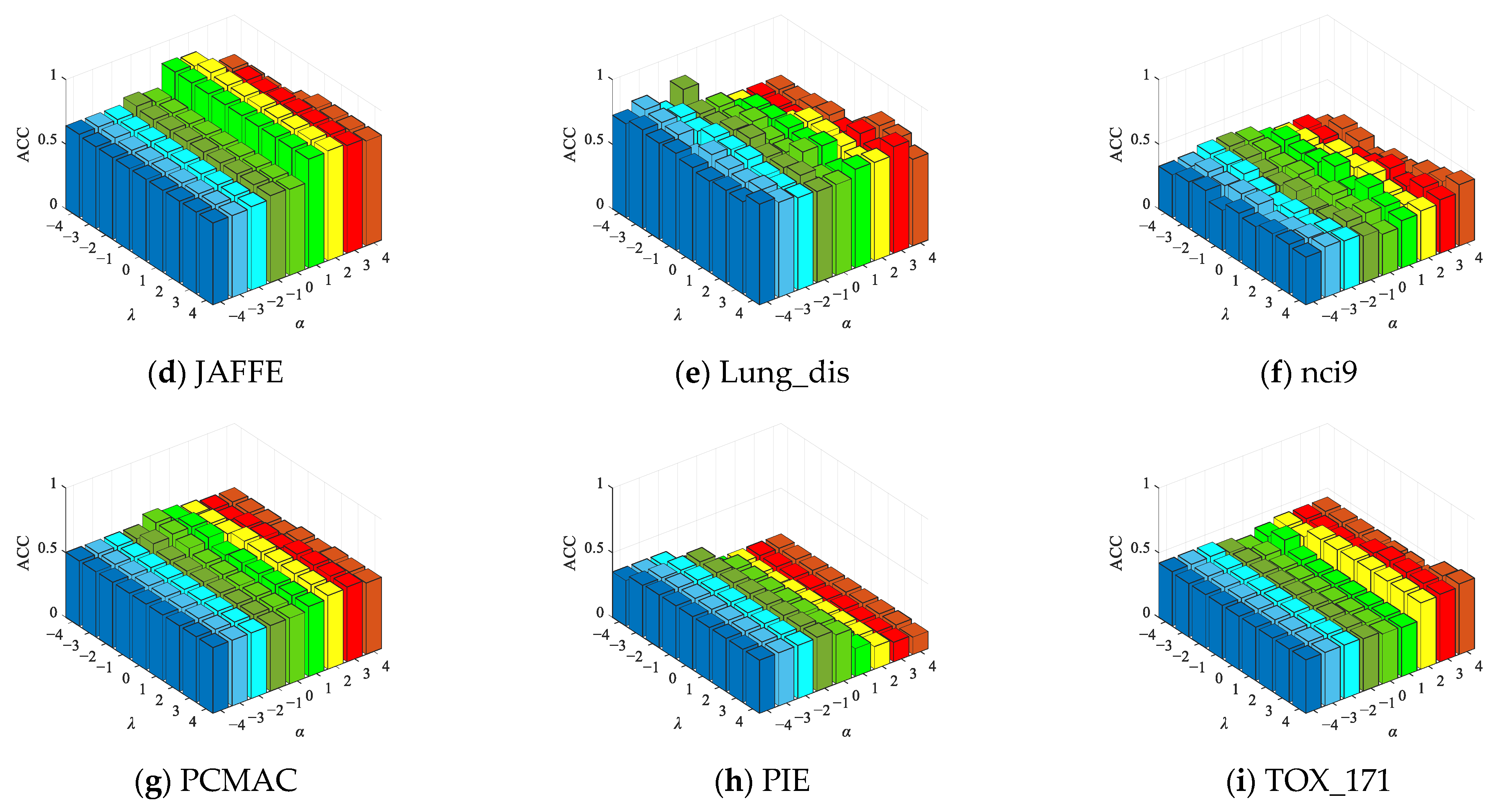
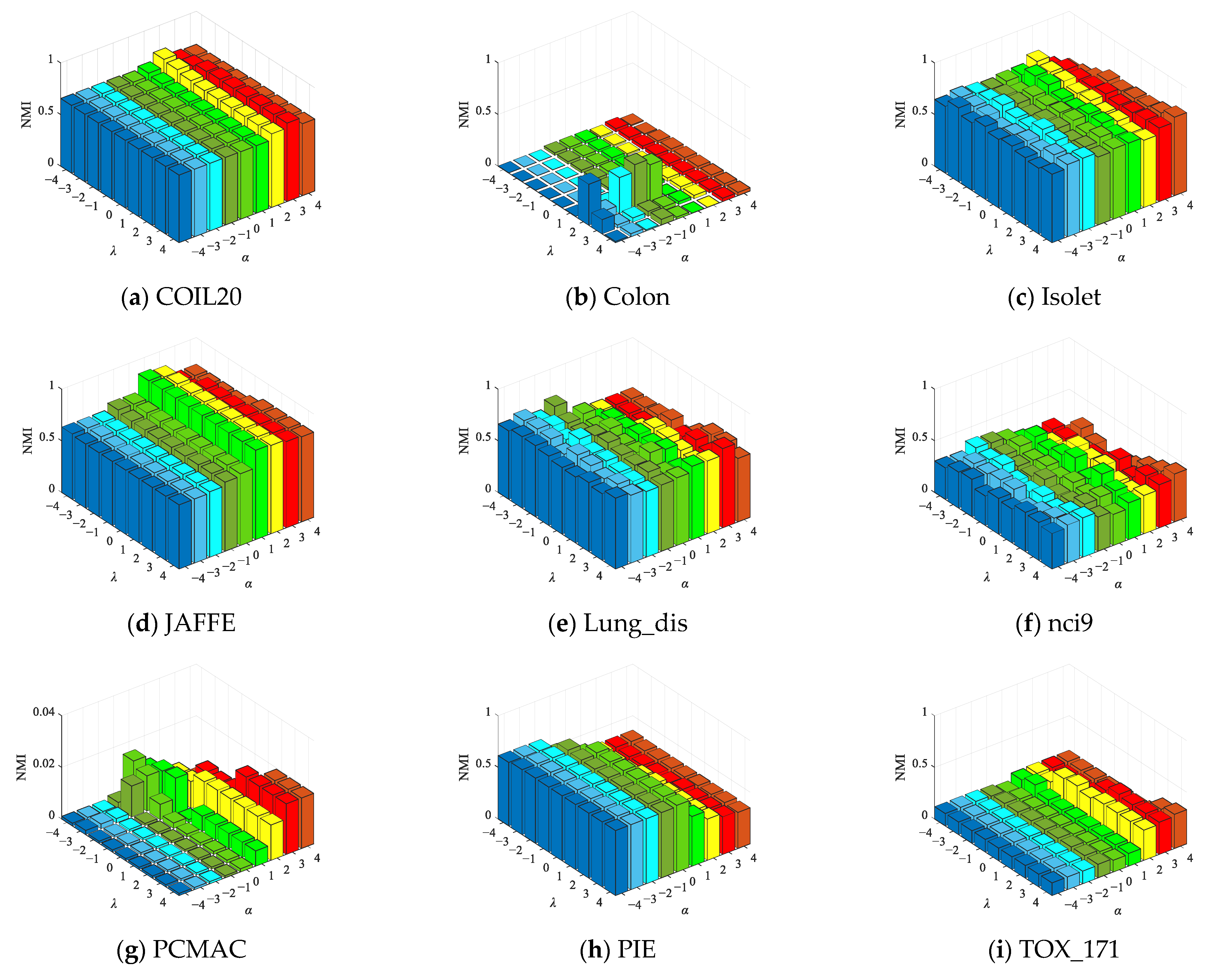
4.6.2. Parameter Sensitivity Experiment
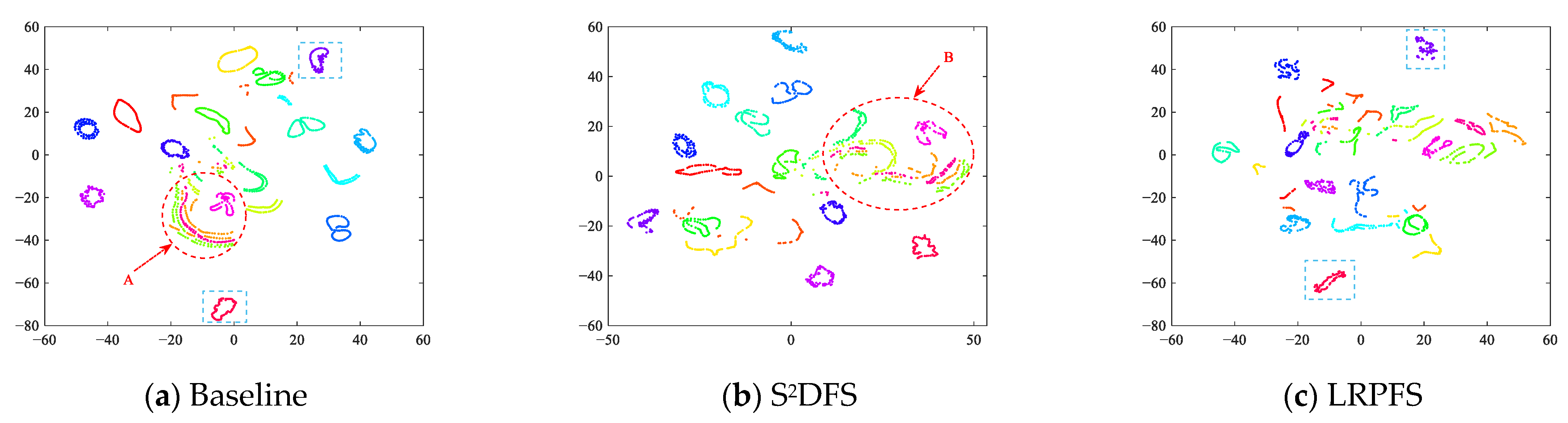
4.6.3. The Effectiveness Evaluation of Feature Selection
5. Conclusions
Author Contributions
Funding
Data Availability Statement
Conflicts of Interest
References
- Jain, A.; Zongker, D. Feature selection: Evaluation, application, and small sample performance. IEEE Trans. Pattern Anal. Mach. Intell. 1997, 19, 153–158. [Google Scholar] [CrossRef]
- Nie, F.; Wang, Z.; Wang, R.; Li, X. Submanifold-preserving discriminant analysis with an auto-optimized graph. IEEE Trans. Cybern. 2020, 50, 3682–3695. [Google Scholar] [CrossRef] [PubMed]
- Lee, D.; Seung, H. Learning the parts of objects by non-negative matrix factorization. Nature 1999, 401, 788–791. [Google Scholar] [CrossRef] [PubMed]
- Lipovetsky, S. PCA and SVD with nonnegative loadings. Pattern Recognit. 2009, 42, 68–76. [Google Scholar] [CrossRef]
- Roweis, S.; Saul, L. Nonlinear dimensionality reduction by locally linear embedding. Science 2000, 290, 2323–2326. [Google Scholar] [CrossRef] [PubMed]
- Li, J.; Cheng, K.; Wang, S.; Morstatter, F.; Trevino, R.P.; Tang, J.; Liu, H. Feature selection: A data perspective. ACM Comput. Surv. (CSUR) 2017, 50, 1–45. [Google Scholar] [CrossRef]
- Saberi-Movahed, F.; Rostami, M.; Berahmand, K.; Karami, S.; Tiwari, P.; Oussalah, M.; Band, S. Dual regularized unsupervised feature selection based on matrix factorization and minimum redundancy with application in gene selection. Knowl. Based Syst. 2022, 256, 109884. [Google Scholar] [CrossRef]
- Wang, Y.; Wang, J.; Tao, D. Neurodynamics-driven supervised feature selection. Pattern Recogn. 2023, 136, 109254. [Google Scholar] [CrossRef]
- Plaza-del-Arco, F.; Molina-González, M.; Ureña-López, L.; Martín-Valdivia, M. Integrating implicit and explicit linguistic phenomena via multi-task learning for offensive language detection. Knowl. Based Syst. 2022, 258, 109965. [Google Scholar] [CrossRef]
- Ang, J.; Mirzal, A.; Haron, H.; Hamed, H. Supervised, unsupervised, and semi-supervised feature selection: A review on gene selection. IEEE/ACM Trans. Comput. Biol. Bioinf. 2016, 13, 971–989. [Google Scholar] [CrossRef]
- Bhadra, T.; Bandyopadhyay, S. Supervised feature selection using integration of densest subgraph finding with floating forward-backward search. Inf. Sci. 2021, 566, 1–18. [Google Scholar] [CrossRef]
- Wang, Y.; Wang, J.; Pal, N. Supervised feature selection via collaborative neurodynamic optimization. IEEE Trans. Neural Netw. Learn. Syst. 2022. [Google Scholar] [CrossRef] [PubMed]
- Han, Y.; Yang, Y.; Yan, Y.; Ma, Z.; Sebe, N.; Zhou, X. Semisupervised feature selection via spline regression for video semantic recognition. IEEE Trans. Neural Netw. Learn. Syst. 2015, 26, 252–264. [Google Scholar] [CrossRef] [PubMed]
- Chen, X.; Chen, R.; Wu, Q.; Nie, F.; Yang, M.; Mao, R. Semisupervised feature selection via structured manifold learning. IEEE Trans. Cybern. 2022, 52, 5756–5766. [Google Scholar] [CrossRef] [PubMed]
- Li, Z.; Tang, J. Unsupervised feature selection via nonnegative spectral analysis and redundancy control. IEEE Trans. Image Process. 2015, 24, 5343–5355. [Google Scholar] [CrossRef] [PubMed]
- Zhu, P.; Hou, X.; Tang, K.; Liu, Y.; Zhao, Y.; Wang, Z. Unsupervised feature selection through combining graph learning and ℓ2,0-norm constraint. Inf. Sci. 2023, 622, 68–82. [Google Scholar] [CrossRef]
- Shang, R.; Kong, J.; Zhang, W.; Feng, J.; Jiao, L.; Stolkin, R. Uncorrelated feature selection via sparse latent representation and extended OLSDA. Pattern Recognit. 2022, 132, 108966. [Google Scholar] [CrossRef]
- Zhang, R.; Zhang, H.; Li, X.; Yang, S. Unsupervised feature selection with extended OLSDA via embedding nonnegative manifold structure. IEEE Trans. Neural Netw. Learn. Syst. 2022, 33, 2274–2280. [Google Scholar] [CrossRef]
- Zhao, Z.; Liu, H. Spectral feature selection for supervised and unsupervised learning. In Proceedings of the 24th Annual International Conference on Machine Learning, Corvalis, OR, USA, 20–24 June 2007; pp. 1151–1157. [Google Scholar] [CrossRef]
- Cai, D.; Zhang, C.; He, X. Unsupervised feature selection for multi-cluster data. In Proceedings of the 16th ACM SIGKDD International Conference on Knowledge Discovery and Data Mining, Washington, DC, USA, 25–28 July 2010; pp. 333–342. [Google Scholar] [CrossRef]
- Hou, C.; Nie, F.; Li, X.; Yi, D.; Wu, Y. Joint embedding learning and sparse regression: A framework for unsupervised feature selection. IEEE Trans. Cybern. 2014, 44, 2168–2267. [Google Scholar] [CrossRef]
- He, X.; Cai, D.; Niyogi, P. Laplacian score for feature selection. In Advances in Neural Information Processing Systems 18; The MIT Press: Cambridge, MA, USA, 2005; pp. 507–514. [Google Scholar]
- Shang, R.; Wang, W.; Stolkin, R.; Jiao, L. Subspace learning-based graph regularized feature selection. Knowl. Based Syst. 2016, 112, 152–165. [Google Scholar] [CrossRef]
- Liu, Y.; Ye, D.; Li, W.; Wang, H.; Gao, Y. Robust neighborhood embedding for unsupervised feature selection. Knowl. Based Syst. 2020, 193, 105462. [Google Scholar] [CrossRef]
- Nie, F.; Zhu, W.; Li, X. Unsupervised feature selection with structured graph optimization. In Proceedings of the AAAI Conference on Artificial Intelligence, Phoenix, AZ, USA, 12–17 February 2016; pp. 1302–1308. [Google Scholar]
- Li, X.; Zhang, H.; Zhang, R.; Liu, Y.; Nie, F. Generalized uncorrelated regression with adaptive graph for unsupervised feature selection. IEEE Trans. Neural Netw. Learn. Syst. 2019, 30, 1587–1595. [Google Scholar] [CrossRef]
- Chen, H.; Nie, F.; Wang, R.; Li, X. Unsupervised feature selection with flexible optimal graph. IEEE Trans. Neural Netw. Learn. Syst. 2022. [Google Scholar] [CrossRef] [PubMed]
- Tang, C.; Bian, M.; Liu, X.; Li, M.; Zhou, H.; Wang, P.; Yin, H. Unsupervised feature selection via latent representation learning and manifold regularization. Neural Netw. 2019, 117, 163–178. [Google Scholar] [CrossRef] [PubMed]
- Shang, R.; Wang, L.; Shang, F.; Jiao, L.; Li, Y. Dual space latent representation learning for unsupervised feature selection. Pattern Recognit. 2021, 114, 107873. [Google Scholar] [CrossRef]
- Samaria, F.; Harter, A. Parameterisation of a stochastic model for human face identification. In Proceedings of the 2nd IEEE Workshop on Applications of Computer Vision, Princeton, NJ, USA, 19–21 October 1994; pp. 138–142. [Google Scholar]
- Yang, F.; Mao, K.; Lee, G.; Tang, W. Emphasizing minority class in LDA for feature subset selection on high-dimensional small-sized problems. IEEE Trans. Knowl. Data Eng. 2015, 27, 88–101. [Google Scholar] [CrossRef]
- Tao, H.; Hou, C.; Nie, F.; Jiao, Y.; Yi, D. Effective discriminative feature selection with nontrivial solution. IEEE Trans. Neural Netw. Learn. Syst. 2016, 27, 796–808. [Google Scholar] [CrossRef]
- Pang, T.; Nie, F.; Han, J.; Li, X. Efficient feature selection via ℓ2,0-norm constrained sparse regression. IEEE Trans. Knowl. Data Eng. 2019, 31, 880–893. [Google Scholar] [CrossRef]
- Zhao, S.; Wang, M.; Ma, S.; Cui, Q. A feature selection method via relevant-redundant weight. Expert Syst. Appl. 2022, 207, 117923. [Google Scholar] [CrossRef]
- Nouri-Moghaddam, B.; Ghazanfari, M.; Fathian, M. A novel multi-objective forest optimization algorithm for wrapper feature selection. Expert Syst. Appl. 2021, 175, 114737. [Google Scholar] [CrossRef]
- Maldonado, S.; Weber, R. A wrapper method for feature selection using support vector machines. Inf. Sci. 2009, 179, 2208–2217. [Google Scholar] [CrossRef]
- Shi, D.; Zhu, L.; Li, J.; Zhang, Z.; Chang, X. Unsupervised adaptive feature selection with binary hashing. IEEE Trans. Image Process. 2023, 32, 838–853. [Google Scholar] [CrossRef] [PubMed]
- Nie, F.; Wang, Z.; Tian, L.; Wang, R.; Li, X. Subspace Sparse Discriminative Feature Selection. IEEE Trans. Cybern. 2022, 52, 4221–4233. [Google Scholar] [CrossRef] [PubMed]
- Roffo, G.; Melzi, S.; Castellani, U.; Vinciarelli, A.; Cristani, M. Infinite feature selection: A graph-based feature filtering approach. IEEE Trans. Pattern Anal. Mach. Intell. 2021, 43, 4396–4410. [Google Scholar] [CrossRef] [PubMed]
- Yang, Y.; Shen, H.; Ma, Z.; Huang, Z.; Zhou, X. ℓ2,1-norm regularized discriminative feature selection for unsupervised learning. In Proceedings of the Twenty-Second International Joint Conference on Artificial Intelligence, Barcelona, Spain, 16–22 July 2011; pp. 1589–1594. Available online: https://dl.acm.org/doi/10.5555/2283516.2283660 (accessed on 8 August 2022).
- Xue, B.; Zhang, M.; Browne, W. Particle Swarm Optimization for Feature Selection in Classification: A Multi-Objective Approach. IEEE Trans. Cybern. 2013, 43, 1656–1671. [Google Scholar] [CrossRef] [PubMed]
- Ding, D.; Yang, X.; Xia, F.; Ma, T.; Liu, H.; Tang, C. Unsupervised feature selection via adaptive hypergraph regularized latent representation learning. Neurocomputing 2020, 378, 79–97. [Google Scholar] [CrossRef]
- Shang, R.; Kong, J.; Feng, J.; Jiao, L. Feature selection via non-convex constraint and latent representation learning with Laplacian embedding. Expert Syst. Appl. 2022, 208, 118179. [Google Scholar] [CrossRef]
- He, Z.; Xie, S.; Zdunek, R.; Zhou, G.; Cichocki, A. Symmetric nonnegative matrix factorization: Algorithms and applications to probabilistic clustering. IEEE Trans. Neural Netw. 2011, 22, 2117–2131. [Google Scholar] [CrossRef]
- Shang, R.; Wang, W.; Stolkin, R.; Jiao, L. Non-negative spectral learning and sparse regression-based dual-graph regularized feature selection. IEEE Trans. Cybern. 2018, 48, 793–806. [Google Scholar] [CrossRef]
- Huang, D.; Cai, X.; Wang, C. Unsupervised feature selection with multi-subspace randomization and collaboration. Knowl. Based Syst. 2019, 182, 104856. [Google Scholar] [CrossRef]
- Xiao, J.; Zhu, X. Some properties and applications of Menger probabilistic inner product spaces. Fuzzy Sets Syst. 2022, 451, 398–416. [Google Scholar] [CrossRef]
- Cai, D.; He, X.; Han, J. Locally consistent concept factorization for document clustering. IEEE Trans. Knowl. Data Eng. 2011, 23, 902–913. [Google Scholar] [CrossRef]
- Pan, V.; Soleymani, F.; Zhao, L. An efficient computation of generalized inverse of a matrix. Appl. Math. Comput. 2018, 316, 89–101. [Google Scholar] [CrossRef]
- Luo, C.; Zheng, J.; Li, T.; Chen, H.; Huang, Y.; Peng, X. Orthogonally constrained matrix factorization for robust unsupervised feature selection with local preserving. Inf. Sci. 2022, 586, 662–675. [Google Scholar] [CrossRef]


| No. | Datasets | Samples | Features | Class | Type |
|---|---|---|---|---|---|
| 1 | COIL20 | 1440 | 1024 | 20 | Object image |
| 2 | Colon | 62 | 2000 | 2 | Biological |
| 3 | Isolet | 1560 | 617 | 26 | Speech Signal |
| 4 | JAFFE | 213 | 676 | 10 | Face image |
| 5 | Lung_dis | 73 | 325 | 7 | Biological |
| 6 | nci9 | 60 | 9712 | 9 | Biological |
| 7 | PCMAC | 1943 | 3289 | 2 | Text |
| 8 | PIE | 2856 | 1024 | 68 | Face image |
| 9 | TOX_171 | 171 | 5748 | 4 | Biological |
| 10 | Yale64 | 165 | 4096 | 11 | Face image |
| Methods | COIL20 | Colon | Isolet | JAFFE | Lung_dis | nci9 | PCMAC | PIE | TOX_171 |
|---|---|---|---|---|---|---|---|---|---|
| Baseline | 65.75 | 54.84 | 61.73 | 82.04 | 73.63 | 40.75 | 50.49 | 24.68 | 44.77 |
| ±4.16 | ±0.00 | ±2.77 | ±5.59 | ±5.26 | ±5.26 | ±0.00 | ±1.09 | ±3.93 | |
| (all) | (all) | (all) | (all) | (all) | (all) | (all) | (all) | (all) | |
| LapScor | 60.41 | 56.45 | 55.83 | 76.74 | 70.41 | 37.58 | 50.23 | 39.00 | 52.81 |
| ±2.11 | ±0.00 | ±2.14 | ±4.58 | ±7.34 | ±3.08 | ±0.00 | ±1.05 | ±0.27 | |
| (100) | (40) | (100) | (50) | (90) | (80) | (50) | (70) | (20) | |
| SPEC | 64.74 | 56.53 | 46.84 | 80.94 | 71.03 | 46.33 | 50.08 | 17.88 | 50.32 |
| ±3.47 | ±0.36 | ±1.89 | ±5.35 | ±5.38 | ±4.17 | ±0.00 | ±0.89 | ±1.31 | |
| (90) | (30) | (100) | (100) | (100) | (50) | (20) | (100) | (90) | |
| MCFS | 64.22 | 53.23 | 56.81 | 85.40 | 81.92 | 45.58 | 50.13 | 27.87 | 43.63 |
| ±3.37 | ±0.00 | ±2.20 | ±4.41 | ±4.80 | ±3.26 | ±0.00 | ±1.48 | ±1.87 | |
| (50) | (60) | (90) | (100) | (80) | (40) | (20) | (70) | (20) | |
| UDFS | 58.71 | 62.26 | 42.65 | 84.55 | 77.60 | 35.25 | 51.02 | 20.74 | 45.06 |
| ±2.14 | ±1.22 | ±1.72 | ±4.10 | ±6.66 | ±2.25 | ±0.39 | ±0.69 | ±4.18 | |
| (100) | (30) | (100) | (100) | (90) | (60) | (30) | (100) | (70) | |
| SOGFS | 57.83 | 61.29 | 45.44 | 86.03 | 76.71 | 42.75 | 52.50 | 36.60 | 49.80 |
| ±2.78 | ±0.00 | ±1.88 | ±4.78 | ±5.50 | ±4.43 | ±0.41 | ±1.01 | ±2.21 | |
| (100) | (30) | (100) | (70) | (90) | (50) | (80) | (30) | (80) | |
| SRCFS | 57.14 | 58.06 | 55.91 | 76.17 | 70.68 | 39.33 | 50.49 | 39.77 | 47.46 |
| ±2.68 | ±0.00 | ±2.04 | ±4.65 | ±5.36 | ±2.98 | ±0.00 | ±1.05 | ±0.29 | |
| (100) | (100) | (100) | (100) | (80) | (90) | (100) | (90) | (100) | |
| RNE | 61.52 | 62.90 | 49.44 | 73.66 | 73.29 | 36.08 | 53.86 | 27.82 | 54.35 |
| ±1.91 | ±0.00 | ±1.51 | ±4.52 | ±5.32 | ±3.56 | ±4.82 | ±0.83 | ±3.64 | |
| (70) | (70) | (70) | (90) | (90) | (30) | (20) | (40) | (80) | |
| inf-FSU | 58.32 | 72.34 | 56.75 | 66.01 | 78.90 | 32.92 | 50.75 | 40.32 | 39.94 |
| ±2.69 | ±0.79 | ±1.35 | ±3.83 | ±6.21 | ±2.85 | ±0.00 | ±1.11 | ±1.02 | |
| (100) | (50) | (100) | (100) | (80) | (100) | (40) | (100) | (30) | |
| S2DFS | 67.10 | 85.56 | 63.64 | 81.46 | 78.70 | 46.50 | 50.08 | 27.79 | 46.55 |
| ±3.18 | ±0.36 | ±2.09 | ±7.67 | ±4.76 | ±4.25 | ±0.00 | ±0.81 | ±2.43 | |
| (60) | (30) | (100) | (100) | (80) | (100) | (30) | (60) | (50) | |
| LRPFS | 69.31 | 87.10 | 66.41 | 86.31 | 82.23 | 47.25 | 57.84 | 41.62 | 54.44 |
| ±3.17 | ±1.17 | ±1.74 | ±3.63 | ±4.53 | ±4.69 | ±0.97 | ±1.43 | ±0.87 | |
| (90) | (70) | (100) | (60) | (60) | (30) | (60) | (70) | (50) |
| Methods | COIL20 | Colon | Isolet | JAFFE | Lung_dis | nci9 | PCMAC | PIE | TOX_171 |
|---|---|---|---|---|---|---|---|---|---|
| Baseline | 76.69 | 0.60 | 76.06 | 83.61 | 69.27 | 37.96 | 0.01 | 48.84 | 24.17 |
| ±1.99 | ±0.00 | ±1.26 | ±3.37 | ±4.21 | ±5.92 | ±0.00 | ±0.62 | ±3.73 | |
| (all) | (all) | (all) | (all) | (all) | (all) | (all) | (all) | (all) | |
| LapScor | 69.67 | 0.97 | 69.45 | 83.45 | 64.86 | 36.49 | 0.58 | 64.51 | 34.93 |
| ±1.18 | ±0.00 | ±0.91 | ±2.28 | ±5.71 | ±1.66 | ±0.00 | ±0.65 | ±0.36 | |
| (100) | (40) | (100) | (50) | (90) | (40) | (50) | (70) | (20) | |
| SPEC | 73.52 | 1.75 | 59.89 | 83.92 | 67.09 | 45.41 | 0.45 | 42.57 | 25.64 |
| ±1.49 | ±0.02 | ±1.38 | ±3.73 | ±3.55 | ±3.64 | ±0.00 | ±0.43 | ±1.49 | |
| (100) | (30) | (100) | (80) | (100) | (40) | (20) | (20) | (90) | |
| MCFS | 74.14 | 0.10 | 69.80 | 85.82 | 74.01 | 45.76 | 0.41 | 50.89 | 19.00 |
| ±1.90 | ±0.00 | ±0.66 | ±2.20 | ±4.11 | ±3.27 | ±0.00 | ±0.69 | ±3.78 | |
| (60) | (20) | (100) | (100) | (80) | (40) | (20) | (70) | (60) | |
| UDFS | 69.43 | 3.12 | 57.41 | 84.95 | 69.80 | 34.99 | 0.11 | 44.13 | 15.78 |
| ±0.99 | ±0.63 | ±0.87 | ±2.69 | ±4.65 | ±2.95 | ±0.05 | ±0.38 | ±5.16 | |
| (100) | (30) | (100) | (90) | (90) | (20) | (30) | (100) | (100) | |
| SOGFS | 70.79 | 7.79 | 61.35 | 88.08 | 70.60 | 42.42 | 2.16 | 58.55 | 28.18 |
| ±1.72 | ±0.00 | ±0.36 | ±2.97 | ±2.57 | ±3.77 | ±0.52 | ±0.53 | ±4.16 | |
| (100) | (30) | (100) | (70) | (100) | (70) | (80) | (30) | (100) | |
| SRCFS | 69.20 | 1.83 | 68.18 | 81.18 | 65.45 | 37.65 | 0.63 | 64.95 | 31.40 |
| ±0.98 | ±0.00 | ±0.98 | ±3.89 | ±4.25 | ±3.32 | ±0.00 | ±0.86 | ±0.30 | |
| (100) | (100) | (100) | (100) | (100) | (80) | (20) | (90) | (40) | |
| RNE | 72.01 | 3.95 | 62.85 | 78.76 | 67.31 | 33.66 | 1.26 | 54.42 | 28.26 |
| ±1.56 | ±0.00 | ±1.01 | ±3.70 | ±4.40 | ±3.73 | ±1.24 | ±0.55 | ±4.07 | |
| (100) | (70) | (100) | (90) | (90) | (30) | (20) | (40) | (80) | |
| inf-FSU | 68.65 | 16.80 | 71.52 | 69.26 | 74.60 | 27.53 | 0.21 | 65.66 | 13.11 |
| ±1.16 | ±0.77 | ±0.58 | ±2.28 | ±5.81 | ±3.30 | ±0.00 | ±0.73 | ±1.17 | |
| (100) | (50) | (100) | (100) | (80) | (100) | (40) | (100) | (60) | |
| S2DFS | 76.33 | 40.70 | 74.75 | 83.85 | 74.43 | 46.55 | 0.29 | 52.64 | 30.18 |
| ±1.43 | ±0.78 | ±0.83 | ±4.07 | ±3.25 | ±4.06 | ±0.00 | ±0.64 | ±2.36 | |
| (80) | (30) | (100) | (100) | (80) | (100) | (20) | (60) | (100) | |
| LRPFS | 76.55 | 41.80 | 75.96 | 86.71 | 76.63 | 47.12 | 2.00 | 64.97 | 35.80 |
| ±1.03 | ±3.10 | ±0.61 | ±2.12 | ±4.38 | ±4.56 | ±0.30 | ±0.48 | ±1.00 | |
| (100) | (70) | (100) | (90) | (60) | (70) | (90) | (80) | (80) |
| Methods | COIL20 | Colon | Isolet | JAFFE | Lung_dis | nci9 | PCMAC | PIE | TOX_171 |
|---|---|---|---|---|---|---|---|---|---|
| Baseline | 24.91 | 0.62 | 19.13 | 1.64 | 0.43 | 2.56 | 3.04 | 99.57 | 7.84 |
| LapScor | 5.83 | 0.38 | 7.96 | 0.95 | 0.35 | 0.47 | 1.75 | 33.24 | 0.94 |
| SPEC | 10.58 | 0.31 | 12.94 | 0.96 | 0.41 | 0.54 | 16.52 | 53.50 | 1.08 |
| MCFS | 5.97 | 1.01 | 8.01 | 1.24 | 0.65 | 2.14 | 2.83 | 30.88 | 1.39 |
| UDFS | 13.94 | 12.43 | 13.41 | 1.48 | 0.52 | 1198.87 | 67.97 | 55.85 | 314.23 |
| SOGFS | 96.53 | 3.09 | 23.73 | 1.98 | 0.86 | 12,137.22 | 608.57 | 58.83 | 929.49 |
| SRCFS | 10.53 | 0.53 | 12.91 | 1.22 | 0.55 | 0.62 | 12.59 | 51.55 | 1.42 |
| RNE | 12.71 | 29.53 | 12.67 | 5.42 | 1.36 | 476.33 | 50.15 | 33.79 | 179.91 |
| inf-FSU | 10.75 | 2.88 | 9.31 | 1.90 | 0.61 | 55.31 | 50.91 | 47.07 | 28.03 |
| S2DFS | 7.21 | 12.80 | 7.86 | 1.77 | 0.65 | 1379.36 | 60.78 | 31.01 | 291.46 |
| LRPFS | 9.27 | 1.24 | 12.83 | 1.19 | 0.41 | 23.24 | 29.56 | 52.40 | 8.66 |
| Methods | Accuracy (%) | Normalized Mutual Information (%) | ||||
|---|---|---|---|---|---|---|
| 8 × 8 Noise | 12 × 12 Noise | 16 × 16 Noise | 8 × 8 Noise | 12 × 12 Noise | 16 × 16 Noise | |
| LapScor | 56.03 ± 3.43 | 58.72 ± 2.96 | 58.32 ± 3.56 | 67.53 ± 1.06 | 69.83 ± 0.84 | 68.82 ± 1.28 |
| SPEC | 63.90 ± 2.78 | 63.78 ± 2.34 | 56.46 ± 2.29 | 72.18 ± 1.23 | 73.35 ± 1.34 | 67.75 ± 0.92 |
| MCFS | 64.01 ± 3.58 | 63.94 ± 2.02 | 61.96 ± 2.45 | 73.69 ± 1.84 | 73.37 ± 1.08 | 70.77 ± 1.06 |
| UDFS | 59.28 ± 2.68 | 63.45 ± 2.49 | 60.85 ± 2.31 | 69.15 ± 1.33 | 73.12 ± 1.17 | 68.27 ± 1.48 |
| SOGFS | 57.19 ± 2.39 | 57.60 ± 2.59 | 57.43 ± 2.88 | 70.41 ± 1.10 | 70.47 ± 0.77 | 69.85 ± 1.60 |
| SRCFS | 57.70 ± 3.19 | 58.20 ± 2.00 | 57.86 ± 2.42 | 69.81 ± 1.50 | 69.87 ± 1.28 | 68.13 ± 1.00 |
| RNE | 62.05 ± 4.12 | 61.63 ± 2.98 | 53.52 ± 2.35 | 72.44 ± 1.62 | 71.74 ± 1.44 | 65.76 ± 0.88 |
| inf-FSU | 57.33 ± 2.52 | 58.01 ± 2.27 | 59.23 ± 2.19 | 69.06 ± 1.12 | 68.07 ± 1.20 | 68.21 ± 1.42 |
| S2DFS | 65.39 ± 3.19 | 65.75 ± 3.94 | 62.39 ± 3.27 | 73.27 ± 1.81 | 73.40 ± 1.88 | 70.76 ± 1.55 |
| LRPFS | 65.95 ± 2.79 | 66.85 ± 2.50 | 62.58 ± 2.21 | 73.71 ± 1.33 | 74.14 ± 1.15 | 70.94 ± 1.28 |
Disclaimer/Publisher’s Note: The statements, opinions and data contained in all publications are solely those of the individual author(s) and contributor(s) and not of MDPI and/or the editor(s). MDPI and/or the editor(s) disclaim responsibility for any injury to people or property resulting from any ideas, methods, instructions or products referred to in the content. |
© 2023 by the authors. Licensee MDPI, Basel, Switzerland. This article is an open access article distributed under the terms and conditions of the Creative Commons Attribution (CC BY) license (https://creativecommons.org/licenses/by/4.0/).
Share and Cite
Ma, Z.; Huang, Y.; Li, H.; Wang, J. Unsupervised Feature Selection with Latent Relationship Penalty Term. Axioms 2024, 13, 6. https://doi.org/10.3390/axioms13010006
Ma Z, Huang Y, Li H, Wang J. Unsupervised Feature Selection with Latent Relationship Penalty Term. Axioms. 2024; 13(1):6. https://doi.org/10.3390/axioms13010006
Chicago/Turabian StyleMa, Ziping, Yulei Huang, Huirong Li, and Jingyu Wang. 2024. "Unsupervised Feature Selection with Latent Relationship Penalty Term" Axioms 13, no. 1: 6. https://doi.org/10.3390/axioms13010006
APA StyleMa, Z., Huang, Y., Li, H., & Wang, J. (2024). Unsupervised Feature Selection with Latent Relationship Penalty Term. Axioms, 13(1), 6. https://doi.org/10.3390/axioms13010006