Article

Identification of the Yield Rate by a Hybrid Fuzzy Control PID-Based Four-Stage Model: A Case Study of Optical Filter Industry

1
College of Management, National Chin-Yi University of Technology, Taichung 411030, Taiwan
2
Department of Finance, Chaoyang University of Technology, Taichung 413310, Taiwan
3
Department of Business Administration, China University of Technology, Taipei City 116, Taiwan
4
Department of Distribution Management, National Chin-Yi University of Technology, Taichung 411030, Taiwan
5
Department of Electronic Engineering, National Ilan University, Yilan City 26047, Taiwan
*
Authors to whom correspondence should be addressed.
Axioms 2024, 13(1), 54; https://doi.org/10.3390/axioms13010054
Submission received: 15 November 2023 / Revised: 21 December 2023 / Accepted: 13 January 2024 / Published: 16 January 2024

Abstract

:
With the vigorous development of emerging technology and the advent of the Internet generation, high-speed Internet and fast transmission 5G wireless networks contribute to interpersonal communication. Now, the Internet has become popular and widely available, and human life is inseparable from various experiences on the Internet. Many base stations and data centers have been established to convert and switch from electrical transmission to optical transmission; thus, it is entering the new era of optical fiber networks and optical communication technologies. For optical communication, the manufacturing of components for the purpose of high-speed networks is a key process, and the requirement for the stability of its production conditions is very strict. In particular, product yields are always low due to the restriction of high-precision specifications associated with the limitations of too many factors. Given these reasons, this study proposes a hybrid fuzzy control-based model for industry data applications to organize advanced techniques of box-and-whisker plot method, association rule, and decision trees to find out the determinants that affect the yield rate of products and then use the fuzzy control Proportional-Integral-Derivative (PID) method to manage the determinants. Since it is unrealistic to test the real machine online operation at the manufacturing stage, the simulation software supersedes this for improved results, and a mathematical neural network is used to verify the given data to confirm whether its result is similar to that of the simulation. The study suggests that excessive temperature differentials between substrate and cavity can lead to low yields. It suggests using fuzzy control technology for temperature management, which could increase yield, reduce labor costs, and accelerate the transition to high-speed networks by mass-producing high-precision optical filters.

1. Introduction

In this section, we describe optical filters and related industrial application research and important problems encountered in the manufacturing process, then explain the purpose of relevant research, and finally introduce the paper structure of this study.

1.1. Research Background with Research Importance

With the development of emerging optical communication network technology, there is an existing need for loading more data and traffic, and it is necessary to make signal transmission faster and more real-time; thus, optical filters have become one of the most important optical communication components. Figure 1 shows the related products for the optical filter industry, which are usually stacked by the physical phenomenon of evaporation. Evaporation is a kind of physical process; it refers to heating the evaporated medicinal materials to a certain sufficient vapor pressure in a vacuum state, so that the medicinal materials are coated with evaporate naturally. Condensation into a thin film layer by layer on the substrate has many advantages, such as simplicity and convenience, fast film formation speed, high efficiency, large coating area, and low cost.
Specifically, the evaporated atomic energy is relatively low, the ionization rate is not high, the binding to the substrate is poor, and the distribution is not good. For narrow-band filters, since the film is thicker and the number of coating layers is more than 200, the evaporated waveform must consider the central wavelength, head width, bottom width, and ripple stability [1], which results in that good products are usually not enough. Therefore, some conditions of the equipment itself must be stable, including temperature control, cooling water system, stable vacuum control, electron gun, ion source, and other related peripherals. It is also an important benefit to have stable water, gas, and electricity around the equipment. These benefits include the process of ice water, such as cooling water temperature, cooling water pressure, cooling water flow rate, and environmental temperature and humidity control, etc., which affect the yield rate of this product.
For the optical filter products, the fronthaul part is the user end for industry applications, such as mobile phones, computers, and driverless cars. The midhaul part is passive components used in the telecommunications room, including fixed networks, area networks, and passive components of optical communication called Edge/Dense wavelength division multiplexing (DWDM)/beamsplitter (BS). The backhaul part is used for the cloud database that passive components of optical communication for optical filters are called Coarse Wavelength Division Multiplexing (CWDM)/Lan-Wavelength Division Multiplexing (LWDM)/Optical Block [2]; thus, optical filters are one of the most important modern network communication components.
With the above statements, the related emerging importance of manufacturing optical filters has piqued a variety of interest in this study for the key topics of the manufacturing process. Thus, these core issues are highlighted as the main research focus, and it becomes the key research object emphasized in this study.

1.2. Research Motivation

With the advent of the high-speed network era, human beings rely heavily on the convenience of the network for different purposes, and the demand for optical components in the market is increasing continually. Smartphones and home computers of various 3C products have connected to the Internet with the function of extensive applications, and these applications related to daily life can no longer be separated from human beings. In 2021, due to more than 200 million people worldwide confirmed with the severe coronavirus disease 2019 (COVID-19) and the death toll reaching more than 4.5 million, many countries will use remote video teaching to avoid human-to-human contact infection; thus, the Internet generation has brought great benefits and convenience to human beings. In order to make the network high-speed and stable, it is an important key point to have a high-speed base station, and thus it is a requirement to have good optical filters for this key point. In addition, with the 5G generation, the demand for optical filters, which are one of the key components used in 5G base stations, is increasing gradually in the application market; more base stations need to be set up around the world to improve the transmission signal. Importantly, optical filters have become so popular that demand exceeds supply now; thus, it is important to improve the yield rate of production to increase the output of optical filter productivity.
The research motivation of this study is to use some effective models or methods, like the main concept of fuzzy set and artificial neural networks (ANN) to better process optical filters for benchmarking their yields for the 5G optical communication industry. Specifically, the processing flow of manufacturing optical filters is very time-consuming; improving the yield rates can directly reduce costs of both manpower and materials and indirectly increase production quantity. Furthermore, the techniques of data mining are developing sustainably. Many factories use data mining techniques to solve problems faced on the production line. For aquaculture production, Gladju et al. [3] used the framework of data mining techniques and machine learning methods to provide a solution for smart decision-making for solving the complex problems of aquaculture and fisheries. In the study of Guo et al. [4], they offered some sub-modules with different MIS (manufacturing management system) functions, such as material management, order management, and assembly line logistics scheduling, or system management, based on data mining techniques in artificial intelligence (AI) for energy-saving resources. In research by Du et al. [5], they optimized a high-dimensional design space for the supercritical CO2 recompression cycle (abbreviated as sCO2-RC) by using deep learning and data mining techniques of machine learning to measure decisional variables for optimizing systems. Moreover, Coşkun et al. [6] used both integrating lameness scores and some image parameters by using a data mining technique to process thermal images with the ImageJ program in order to measure the early detection of lameness in Brown Swiss cattle. Clancy et al. [7] provided a method to decide a methodology to enable data-driven quality management in order to reduce the waste from manufacturing processes using data mining techniques. A study by Tu et al. [8] explored the principles and characteristics of acupuncture for treating major depressive disorder (MDD) by analyzing its clinical trials using data mining techniques. Chien and Chuang [9] made a detection framework for batch processing systems of semiconductor manufacturing by a big data mining analysis, and in the study of Lyu et al. [10], they used a data analysis membrane filter by a data-driven approach to identify possible manufacturing processes and production parameters that lead to defects in produced products.
From these documents in the literature review above, we understand that data mining techniques used for industrial data analysis bring convenience and important benefits to all walks of life and industry applications, particularly for improving the yield rate of the manufacturing industry. Thus, for the data mining learning techniques, it should be an effective trigger-based challenge used to underline the research importance of this study to trigger with the more data-driven models in advance to identify potential industry applications for lowering manufacturing process costs from highlights on optical filter industries.

1.3. Research Gap and Research Question

According to the problems faced in the production of optical filters [11], the manufacturing process is limited by the need for longer time, machine working conditions, quality of raw materials, and stable peripheral equipment, such as electricity, temperature and pressure of cooling water, air pressure, the status of the central air conditioning system, humidity control, water quality, etc. Production needs also include the design of the coating program and the operating skill of the operator. If one of these requirements is not met, it will affect the output yield rate. Interestingly, past research has studied evaporation machines for measuring the electricity, water, and gas of a factory and found that it is better for the manufacturing process when the water temperature is set at 19–21 degrees, the cooling water pressure is set at 2.6–3.0 kg, the cooling water conductivity is set at 151–200 um/cm, and the air pressure is set at 4.1–4.5 kg. However, these are only the experimental results of the manufacturing process for the requirements of the factory service, and there is still a lack of controllable data from important features related to other equipment. Notably, this study proposes the use of an effective method to add some useful conditions to the manufacturing process and collects more real data to be further explored to benefit some manufacturing operations from further analysis. In particular, the controllable conditions of the evaporation equipment are the key to success in correctly identifying the yield rate of output, and the product of the optical filter is a high-precision part processed; each link in the manufacturing process is very important. Given the above reasons, this study emphasizes how to improve the yield rate of optical filters for evaporation manufacturing to outline these emerging areas of industry application-oriented research. It is a major objective for this study that we are dedicated to finding out the related conditions and resources, including production time, product type, production equipment, substrate size, substrate temperature, cavity temperature, the temperature difference between the substrate and the cavity, the cooling water temperature, the cooling water pressure, status of yield, distribution of yield, analysis of failure causes, and the adjustment references of the light spots of the two medicinal materials, etc., when the manufacturing process is handled. We propose an effective mathematical model with some components and corresponding work: (1) To further identify more than thousands of collected raw data points and analyze them with a valuable data mining technique such as the distribution status of box-and-whisker plots (abbreviated as boxplots) and the analysis of association rules, (2) to find out the related problems faced and the correlation or associativity between good products and bad products by using a decision tree model, and (3) to then use effective control methods, such as intelligent control, fuzzy control, and neural networks (NN), to solve and improve the critical problems. Thus, we have three important steps to take to implement the proposed model. (1) The study first uses the control system of evaporation manufacturing and establishes a mathematical factory model. (2) Then, mathematical software and circuit software are used to imitate the factory structure to simulate the evaporation process of an optical filter. (3) During the simulation process, we process the data changes of some collected features, collect further relevant information from the manufacturing process, and use the ANN to confirm the effectiveness of the research, correct the factors that cause adverse effects of products, and gradually increase the yield rate.
This study is motivated by exploring the potential challenges of the optical filter’s manufacturing process and thereby studying an interesting and important issue for both academics and industry practitioners meaningfully.

1.4. Research Purpose

This study collects thousands of real data points produced by the process of evaporation in order to measure the proposed hybrid model; accordingly, this study has the following major research purposes to identify and overcome the issue of yields:
(1)
Propose an efficacious hybrid model to properly identify the yield rate with the main objective of reducing the output of defective products, which can not only directly save production time and reduce labor and material cost losses but also indirectly increase the number of outputs in the operating process of manufacturing optical filters.
(2)
Use package software for big data mining techniques to analyze the given real data to find out the regularities related to the yield.
(3)
Use the empirical method of research experiments to create the association rules to discover the problem of poor production.
(4)
Find the suitable control methods of fuzzy control, intelligent control, and the NN model to further identify the manufacturing problem of optical filters.
(5)
The main purpose of this study is to improve the yield rate of optical filters quickly and effectively.

1.5. Research Structure

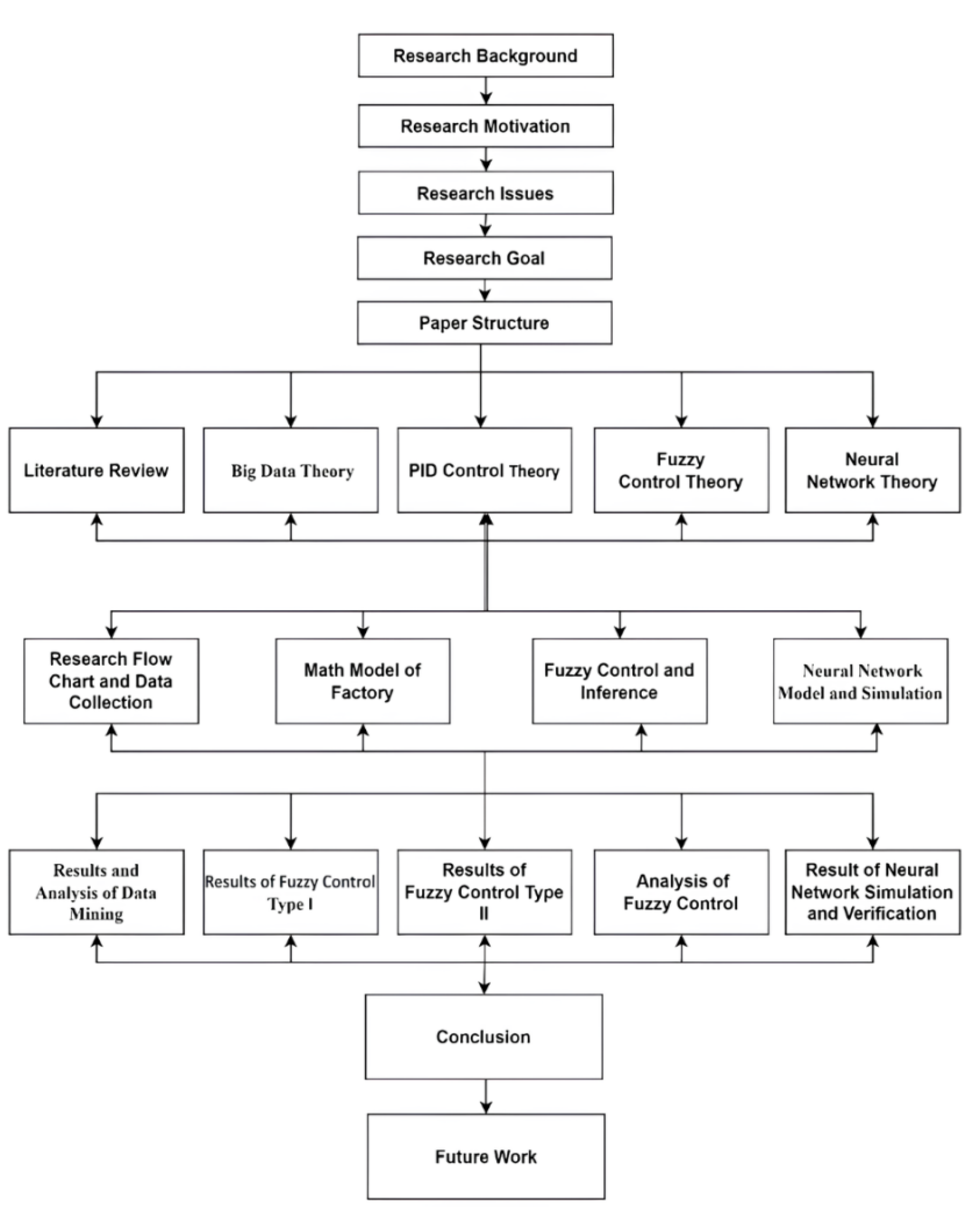
The structure of this study has five sections, described as follows: Section 1 mainly discusses the background and relevant problems of addressing the production line to reduce the occurrence of defective products, as well as highlighting the purposes of the study. The second section is to describe the literature review and theoretical background of this study. Section 3 describes the main research methods and techniques used for this study, mainly box-and-whisker analysis, association rule analysis, decision tree analysis of a data mining technique of machine learning, fuzzy control method, and NN model. Section 4 is to analyze the empirical results and effectiveness of the research through experimental examples. The final section concludes the study results from a variety of empirical analyses with a discussion of differences and prospects for future research from experiencing this empirical work. The research flowchart for the study is shown in Figure 2.

2. Related Work

This section is to make a literature review of relevant industrial applications and theoretical backgrounds of this study, including industrial background and applications of optical communication thin film filters, related data mining techniques and applications, Proportional–Integral–Derivative (PID) control theory and applications, fuzzy control theory and applications, and NN theory and applications.

2.1. Industrial Background and Applications of Optical Communication Thin Film Filters

Optical communication thin film filter is a type of thin film filter, and its manufacturing process is to use the principle of thin film evaporation, to use the method of physical gas deposition, and to use the principle of dielectric material to apply two kinds of medicinal materials SiO2 and Ta2O5, which are exchanged layer by layer using the high voltage and low current of the electron gun. This generates high-voltage arcs, shooting on the medicinal materials [12,13,14,15], melting under vacuum to generate airflow heat convection, and so attaching the medicinal materials to the steam. The size of the substrate has three specifications: 95 mm, 150 mm, and 228 mm in diameter, and the number of evaporated layers of the finished product can be 200–300 layers. By controlling the thickness of the coating film and the sequence of the arrangement, the wavelengths required by customers can pass through, and different wavelengths are filtered out when the light passes through the filters of different products. Therefore, it is possible to achieve the effect that a single optical signal source is divided into multiple project channels. Due to the continuous increase in the number of channels requested, the evaporated layers need more than a hundred layers, and thus the manufacturing of optical filters is very difficult for achieving sufficient yields to lower operating losses. Practically, optical filters are often used for the well-functioning dense wavelength division multiplexer (DWDM) with over 8 channels. Due to the different uses, specifications, channels, or wavelengths, many derived items are created for the categories of optical filters. As for the application fields, it covers a wide range of domains, such as optical communications, optics, medicine, lasers, and space science. The following descriptions of different components for optical filters are their relevant basic applications:
(1)
The DWDM system is a very efficient optical transmission method that can accommodate more than four channels under the conditions of the original optical fiber equipment. Thus, its most important application is focused on the use of a backbone network. Due to the fact that DWDM is mainly used in the backbone network, the transmission capacity has increased by more than four times. As for the lack, this system uses several different wavelengths to share a single optical fiber, resulting in a technical difficulty for manufacturing.
(2)
Coarse wavelength division multiplexer (CWDM) is also a direct way for the purpose of optical transmission; it uses the thin-film filter technique for optical fiber transmission modules, so it only accommodates two channels, and their wavelength spacing can be compared. Its new-generation design is directly applied to the optical transceiver module at the end of use, and its usage will far exceed the speed of the LAN. CWDM is mainly used in post-transmission cloud databases and LAN use-site transceiver modules. It has the benefits of low technical difficulty, small data transmission volume, and low manufacturing cost, but it has two features: only two channels and wavelength spacing as large as 20 nm.
(3)
Gain flattening filters (GFFs) are mainly used to compensate and make the signal more stable. Raman fiber amplifier (RFA) provides a wide gain bandwidth of up to 100 nm. Erbium-doped fiber amplifier (EDFA) on broadband can extend the transmission distance. Currently, they can be applied in the system for combinations of three networks.
(4)
Band separators filters (BSFs) are optical carrier signals of different wavelengths on various signals. At the sending end, they will be integrated by a multiplexer and coupled to the same optical fiber to make the transmission. The optical signals of various wavelengths are separated by a demultiplexer at the receiving end.
(5)
Broad band pass filter (BBPF) and narrow band pass filter (NBPF): they can be used for CWDM and CWDM to improve the quality and bandwidth of the system.
(6)
Anti-reflection coating (ARC) is an optical thin-film filter. Usually, the coating on the reverse side is called the AR side, and the coating on the front side is called the coating side of the product. Its applications can be extended to digital cameras, projectors, cameras, medical instruments, camera lenses for mobile phones, telescope lenses for viewing astronomy, and special eyeglass lenses, as well as optical films necessary for various optical components.
(7)
The edge filter is a multiplexing wave splitter (WDM) for each band; it can be regarded as the function of a switch in application. Thus, it can pass certain wavelengths or prevent certain wavelengths from passing. This is a variety of optical filters required for fiber-to-the-user (FTTx), optical transceiver modules, and passive optical networks (PON), and it is also very commonly used in the industry.
Interestingly, we can connect several computers in a factory or company’s office or at home via ultra-broadband wireless, and this is called a local area network [16,17]. We can also connect the computers in the whole city, and this network is called the backbone network; however, these backbone networks must be approved by the country before they can be directly connected to the Internet abroad. Subsequently, it is only possible to use the Internet through these backbone networks. Thus, it implies that optical filters are very important to the era of the Internet, simultaneously, it is needed to understand how to process and highlight the optical filters.
Figure 3 shows the flow chart of the main processing for the production of optical filters. From Figure 3, it is indicated that when the materials first enter the manufacturing factory, the substrates are cleaned by ultrasonic waves and coated with an anti-reflection coating (i.e., AR coating), and then the substrate is ground and degraded. Thick processing for the coater is coating the surface. Then, the coated substrate is cut into optical filters, and the optical filters are taken out for measurement; if the specifications meet the standards, they can be accordingly packaged and shipped.

2.2. Related Data Mining Techniques and Application

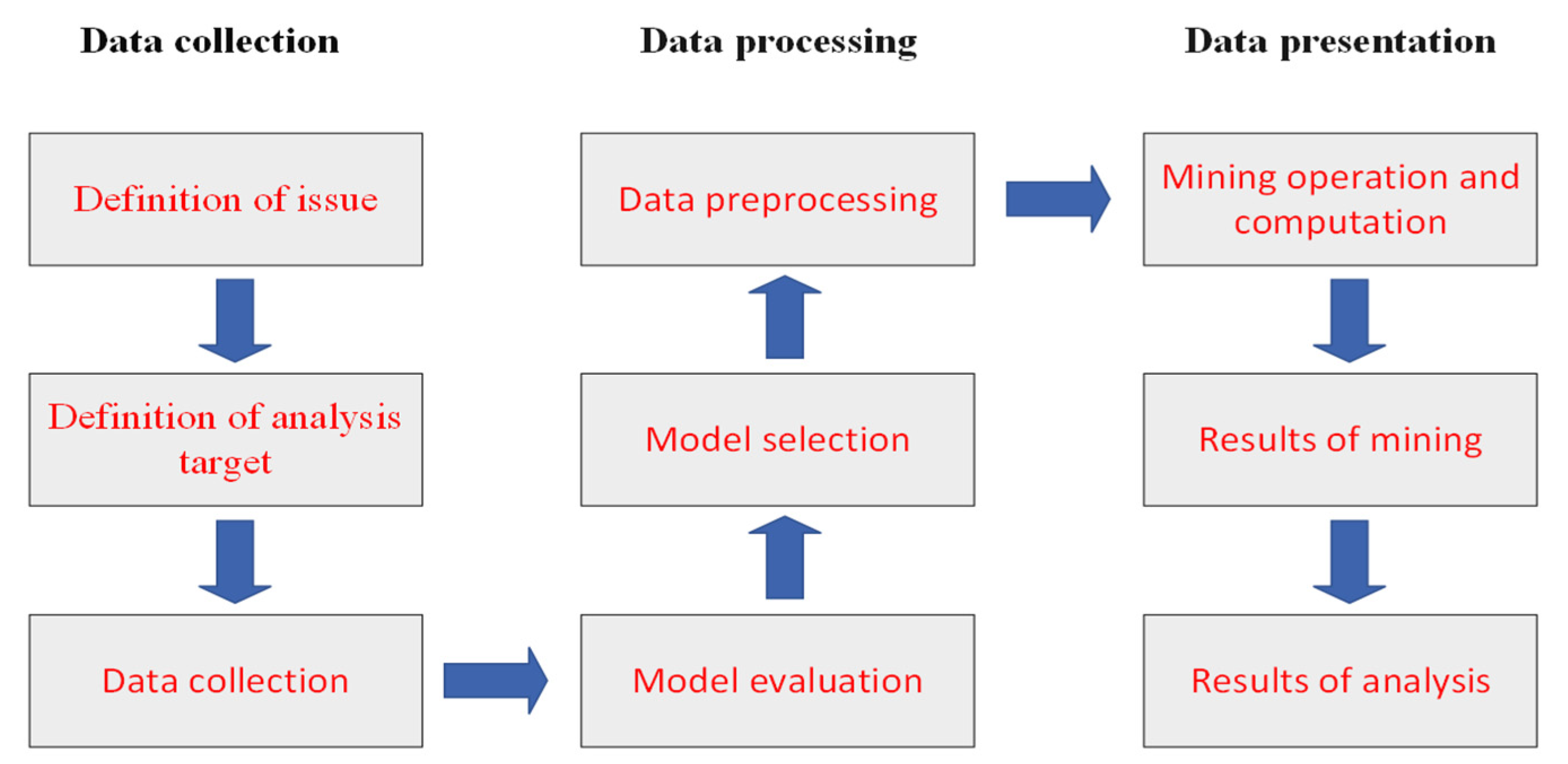
Data mining is an effective process that involves the functions of data collection, data warehousing, and computer processing to analyze a given large raw dataset from real-life problems faced in order to identify potential relationships, uncover trends or patterns, and extract valuable information and knowledge. Figure 4 presents the flowchart of the data mining method. From Figure 4, we can see that the data mining process for a real-time processing framework can be divided into three main stages: the ordering of data, data processing, and data presentation [18]. Furthermore, as to the many functions of data mining techniques, three brilliantly technical methods, including box-and-whisker analysis, association rule analysis, and decision tree classifier, have become the frameworks of professionally emerging models or technologies for challenges and alternatives in industry applications, and thus they are selected and emphasized in this study. The three stages are described in detail as follows, and the three techniques are introduced in the following three subsections, respectively.
(1)
Data collection: For industry application, first clarify the problem to be solved, analyze the definition and structure of the problem, know how to set the data analysis goals, and further collect relevant data from industries for facilitating the setting conditions of experiments to achieve the pre-established objectives like yields of production outputs.
(2)
Data processing: After collecting and organizing a large amount of industrial data, we accordingly employ appropriate tools and suitable models to further analyze the defined problem and dig out useful information about decisional features like association rule algorithms from the given huge amount of data.
(3)
Data presentation: Based on the information obtained from the results of data analysis, find out the insights of empirical results, and then apply visualization presentation or communication analysis to further formulate appropriate action plans to assist decision-making in industry for purposes of improvement.

2.2.1. Box-and-Whisker Analysis

The result of box-and-whisker analysis is a box plot as a visual tool and a very simple and easy-to-understand statistical method, which has a statistical graph showing the distribution of data with a combination of the maximum, minimum, median, first quartile, and third quartile. In particular, the difference between the first quartile and the third quartile is called the interquartile range (IQR), which is commonly used to assess the variability of statistical dispersion. Thus, when drawing a box-and-whisker plot, it is necessary to first determine the fence; the fence is the first quartile −1.5 × IQR and the third quartile +1.5 × IQR. Importantly, this kind of box plot can be learned and interpreted easily and clearly from the outcome of statistical charts; with the helpful benefit that box-and-whisker plots have a wide application field, such as the analysis of lung data in medicine [19] and the data analysis in stores [20].
By highlighting industry applications, this study thus selects it to judge and visualize the distribution features of the given data and benefit the outcome by resulting in a measurable improvement.

2.2.2. Association Rule Analysis

Association rule analysis refers to searching and analyzing events or records that occurred concurrently through some given real data, and the analyzed results can reveal some associated rules for a real-life problem. For example, in a practical purchase record of supermarket customers, it is found that if customer A bought beer, then this customer also bought diapers simultaneously; thus, the beer and diapers form a relevant link, which is called an association rule [21]. Even if a customer buys diapers, there is still a high chance that he or she will also buy beer at the same time; however, it can practically help supermarket decision-makers further formulate a set of cross-selling strategies in order to accelerate the promotion of related products by using the association rule constructed. That is, the operator can change the way that the store is displayed to make it easier for customers to purchase the related products and further increase the probability of sales. In addition, fuzzy association rules (FARs) are a variant of association rules, and they can be used for a variety of industry applications, such as using FARs to find out the power energy loss analysis to achieve the effect of energy savings [22] and using association rules to judge the cause of transformer faults and improve production efficiency for making the power transformer fault diagnosis [23]. In mining, the process of association rules includes two main phases, its key functions are described as follows:
(1)
In the first phase, all high-frequency project groups must be found from the original data collected to set the interval number of equal-frequency discretization in the default discretization, which can be slowly adjusted to a suitable demand value or can be selected to set equal-width discretization, and then complete the setting of individual attributes. The high frequency means that the frequency of a certain item group must reach a certain level relative to all records. The frequency at which an item group appears is called the support degree. To further define frequency, if we take two projects, A and B, we can obtain the support degree of the project group containing A and B. If the support degree is greater than or equal to the set minimum support threshold value, then A and B are called a high-frequency project group. A K-itemset that satisfies the minimum support is called a high-frequency K-item group, which is generally expressed as a large K or a frequent K. The algorithm generates a larger K + 1 from the large K item group, and the search will not stop until no high-frequency item groups can be found and generated.
(2)
Accordingly, the second phase is to generate association rules. First, set the appropriate parameters of high-frequency item groups, such as equal-frequency discretization and interval number, which are based on the previous step for high-frequency K-item groups used to generate rules. If the reliability calculated by a rule satisfies the minimum reliability, this rule is just an association rule.
More importantly, due to the complexity of the production process of optical filters, it is a nonlinear system, so this study uses the characteristics of association rules to formulate its relevant regulations in order to obtain good classification results.

2.2.3. Decision Tree Classifier

In machine learning fields, a decision tree is a good predictive model in a variety of applications; it is a mapping feature between object attributes and object values. Each node in the tree represents an object, and each branch path represents a certain attribute value. The node of each leaf corresponds to the value of the object represented by the path experienced from the node at the root of the tree to the leaf node. A decision tree can generate and learn a decision-making tree-based structure from given data. In particular, for its application, it has many benefits in industrial domains, such as analysis of distribution line fault causes [24], real-time migration of fault trees to decision trees for fault detection at the International Space Station (ISS) [25], misconfiguration detection usage analysis for addressing large-scale cloud data centers [26], etc.
For the illustrious classifier, it has some key algorithms with various advantages, such as classification and regression trees (CART), C4.5, and C5.0.
(1)
CART: The Gini coefficient (abbreviated as Gini in this study) [27] is a statistical measure of inequality on a scale between 0 and 1, indicating that the higher the value, the higher the inequality; thus, it can be used as the criterion for determining the branch variables. Each branch node is separated from the data, and a dichotomous tree structure of decision is established to find out the critical branch variables. Given the features of the binary branching CART algorithm, it can deal with classification problems by benefiting categorical variables and continuous variables. First, given a node t, the branch variable is divided into two elements by the Gini, assuming that the branch level of the attribute is s, t l e f t and t r i g h t are the left and right child nodes of the node t, respectively, and the purity before and after the branch is compared with their difference, G i n i s , t is an increment under the s , t of the Gini, which is formatted as in Equation (1):
Δ G i n i s , t = G i n i t [ G i n i t l e f t + G i n i t r i g h t ]
(2)
C4.5: In C4.5, the ratio of information gain [28] is used as the criterion for determining the branch variables with a multi-branch. In practice, the C4.5 algorithm is most commonly used to handle categorical data, but in the case of continuous data, it first needs to be converted into a category variable. Compared with these features of prediction accuracy, complexity degree, tree pruning, and training time for other classifiers or algorithms, the C4.5 decision tree algorithm provides better advantages in classification accuracy and data interpretation ability.
(3)
C5.0: Its core algorithm for C5.0 [29] is a modified version based on C4.5. C5.0 adopts the concept of pessimistically estimating the classification error rate and directly uses the results of training data to estimate the classification error rate. The confidence level (CL) is a measure of the mean of a certain variable and is formatted as Equation (2); where p represents the probability of misclassification of the leaf node, N is the number of data points in the node t, x represents the number of data that may be misclassified in the node, and E represents the maximum number of data in the node that is misclassified.
C L = x = 0 E C x N p x ( 1 p ) N x
Due to the strong industrial applicability of the decision tree classifier, specific advantages make the utilization rate in learning industrial applications much higher than other algorithms. Therefore, this study applies this classifier to identify practical classification problems with good research results in the real world, such as the problem of filter production processes.

2.3. PID Control Theory and Its Application

For a PID controller, P is proportional, I is integral, and D is differential. Its attributes can be adjusted by adjusting the three benefits of K P , K i , and K d [30], which is common in automatic controls. One of the control methods, such as multi-mecanum-wheeled mobile robot [31], wind power generation system [32], heat exchanger [33], vehicle active suspension based on road [34], water and fertilizer control system [35]. PID control is used for automatic control to improve stability. It is mainly divided into three key functions, described as follows:
(1)
The P controller is a very simple control method. The output of its controller is proportional to the input error signal, and the control amount of proportional control is proportional to the error. When the error is large, the control amount will be relatively large, and the response will rise quickly. Although proportional control can quickly reduce the error, the biggest problem is that when the control amount is less than a certain value, the goal cannot be achieved, and it will cause a steady-state error. This error will not be eliminated by proportional control over time, so it will be presented in the paragraph below. Its proportional control is formatted as Equation (3).
u t = K p e ( t )
(2)
The I controller is the output of the controller and is proportional to the integral of the input error signal. How can the steady-state error be eliminated? It will continue to accumulate the value of the error, so that the control amount will increase. As time increases, the integral term will become larger. If the error is small, the integral term will also increase with time, but if the value is large, the value will keep rising. Finally, under the action of this mechanism, the steady-state error is successfully eliminated, and the output of the controller is increased to further reduce the steady-state error until it is equal to zero and the target value can be reached. Therefore, the proportional + integral (i.e., PI) controller makes the system have no steady-state error after entering the steady state. The integral control is cumulative error and directly added to the control quantity for the integral error function, and its formation is defined as Equation (4).
u t = K p e t + 1 T 1 0 t e ( t ) d t
(3)
The D controller, also an output controller, is directly proportional to the differential of the input error signal; that is the rate of change of the error. Differential is the function of dealing with interference sources. If the machine equipment is affected by external forces and changes rapidly, the error will also increase rapidly. At this time, the differential control can show its unique ability. The differential controller calculates the rate of change of the errors. When the rate of change fluctuates rapidly, the amount of differential controller will increase with the increase in the rate of change of the errors, so that more force will be quickly returned to the target position, making it more stable. When the target is close, the error decreases rapidly, so the derivative of the error is negative. The item function for the differential controller will reduce the control amount, making the speed smaller to prevent exceeding the target value. In summary, the integral controller provides a certain inertia, but the differential controller provides a certain damping; this is the understanding of a simple and intuitive PID controller. The proportional + differential (i.e., PD) controller can suppress the control effect of the errors in advance to be equal to zero or even a negative value, thereby avoiding serious overshoots of the controlled quantity. The PD controller can improve the dynamic characteristics of the system during the adjustment process. The differential control, to calculate the rate of change of the current errors and add it to the control quantity, is defined as Equation (5).
u t = K p ( e t + 1 T T 0 t e t d t + T D d e t d t )
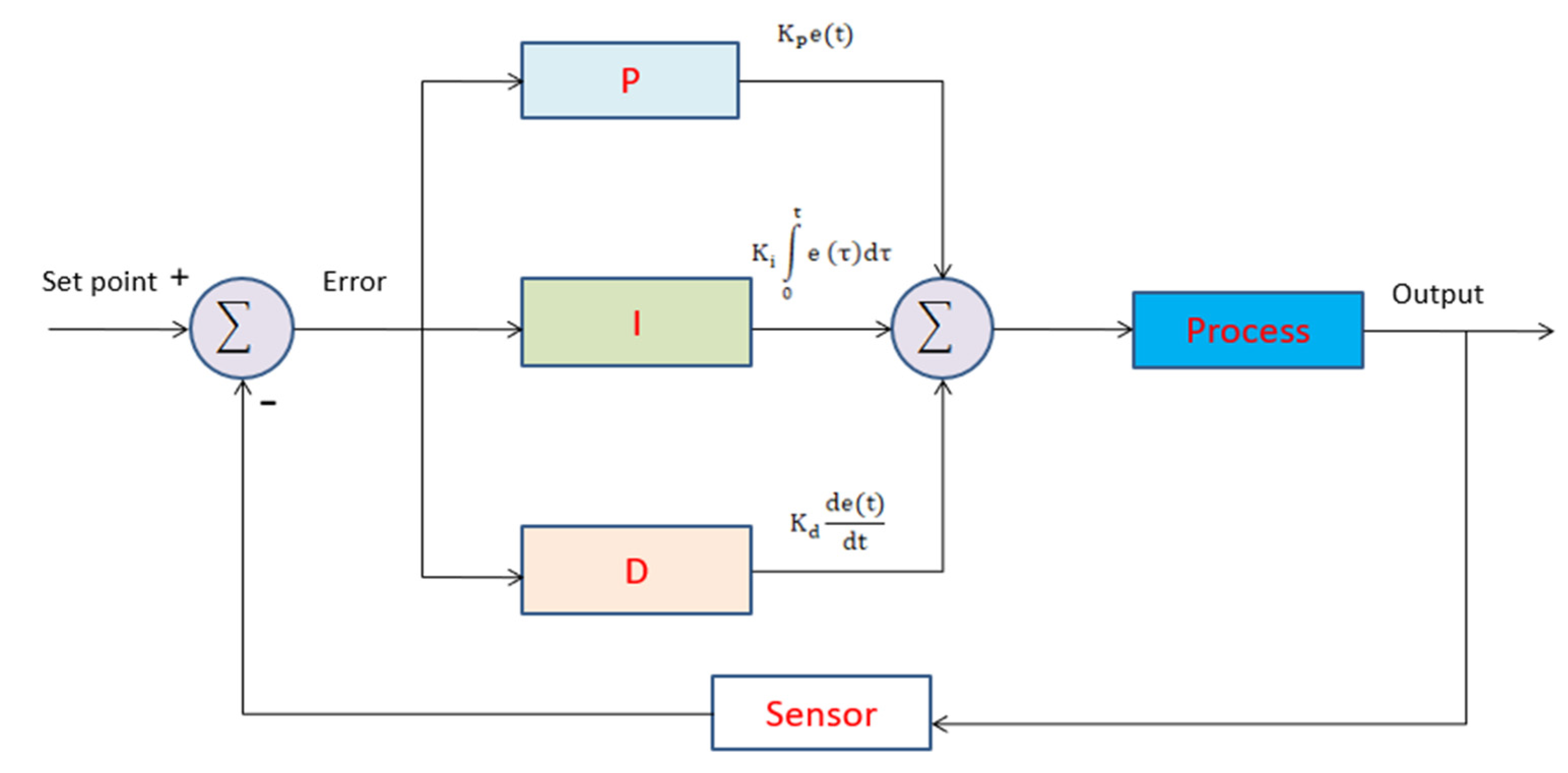
Figure 5 shows the output signal of the closed-loop control system for the PID thermostat. The output signal is fed back to the reference input signal through the sensor to adjust the proportional, integral, and differential values for the total value. After processing, it is inputted and returns to the setting after the input point to compare the error and correct the P, I, and D again until the temperature of the output value is close to the error value. The algorithm is formatted as Equation (6) below, and the steps are as follows: (1) The input signal is the heating current and the actual temperature; (2) the output has the three internal parameters, including P, I, and D, and can be adjusted up, but it is not adjusted down for the three regulation methods.
K p e + K i e d t + K d d e d t

2.4. Fuzzy Control Theory and Its Application

A fuzzy control system mainly has three data inputs, and after fuzzification, the adjustment of empirical rules is established by fuzzy rules, and after defuzzification, the results for output data come out. The basic structure of the fuzzy system has four functions, as follows:
(1)
Fuzzifier: Its function as a fuzzifier is to convert external input data into semantic fuzzy information that can be communicated in the fuzzy system. That is, convert the given “data” to useful “information”. The measurement value of the interface is used to carry out the quantification work, so that this value is transformed into the range of language variables and other pairs [36].
(2)
Fuzzy-rules base: The fuzzy-rules base is composed of a collection in the form of IF-THEN statements that store the human operator’s practical knowledge of the process. The rule base will be more flexible to calculate accurate prediction values. If the rules of the fuzzy-rules base are set well, the calculated results will be more accurate. This kind of fuzzy rule is used to describe the relationship between the input and output of the system; multiple inputs can be set according to the requirements, and a system with multiple outputs can be set according to the requirements.
(3)
Fuzzy inference engine: This engine is the core of the fuzzy system, which can simulate human thinking and decision-making to determine the value. By means of approximate inference or fuzzy inference, it can be used to solve real-life problems.
(4)
Defuzzifier: Defuzzification is the opposite activity of the function of the fuzzification process. Defuzzification must convert the inferred fuzzy output into a real and clear value to communicate with many external interfaces and facilities; that is to be able to find an unambiguous value suitable for representing fuzzy sets. (Note: the defuzzification in this study uses the approach of the center of gravity.

2.5. NN Theory and Its Application

The architecture diagram of basic backpropagation NN (BPNN) [37,38] is a good algorithm that simulates the nerves of organisms; it is composed of an input layer, a hidden layer, and an output layer. A connection in each layer represents a weight; when the weight reaches the threshold through the activation function output, the neuron is activated, and the data is passed to the next layer. The linear activation function can effectively deal with the problem of gradient disappearance. This form is the prototype of BPNN, and the meanings of each layer are described as follows: (1) Input layer X: It is an input set. (2) Output layer Y: It is an output set. (3) Hidden layer: It has a processing function F and the number of neurons; its constructional algorithm will determine the number of hidden layers, and it is dependent on the complexity of the problem faced, increasing from one layer to several layers. (4) Activation function: An input value is directly transmitted from the input layer to the hidden layer, and after the weight is accumulated, an output value can be converted through the activation function, and then it is passed back to the output layer.
In the learning process of the backpropagation (BP) algorithm, the data is composed of forward propagation and negative propagation, respectively, and the input can be obtained from the output through the weighting function (F). In the reverse transfer NN, the input value of the current calculation neuron is the output value of the previous neuron, and the output layer y j n of the NN can be calculated by Equation (7). In the Equation (8), n e t j n is expressed as the weight accumulation of the output value in the n − 1 layer of the network, and w j i n represents the jth neuron of the ith neuron in the n − 1 layer in the n-layer. In this study, the backward transfer neural architecture belongs to the supervised learning method, and the target value b is used as the purpose of learning so as to reduce the error between network input and target output.
y j n = f i w j i y i n 1 = f ( n e t j n )
n e t j n = i w j i n y i n 1 + b j n
In addition, after calculating the function of error (E), its purpose is to reduce the gap between the actual output and the target output, so that the network can correct the output network through E, and the process of making the minimizing E becomes the function of network. The learning process for the network is to process the minimizing the function of error E, and E can be represented by the following Equation (9). Among them, E can be regarded as the correction of the error function, d k is the target output value of the neuron at position k, and y k is the actual output value of the neuron network at position k. In the process of minimizing E, the network will adjust the size of the weight value each time the training data is input.
E = ( 1 2 ) K ( d k y k ) 2
In Equation (10), Δ w j i is the adjusted weight, and the degree of adjusted change is proportional to the weight connection value. η is the learning rate, usually set between 0.8 and 1.2.
Δ w j i = η E w j i
In reviewing many studies, such as optimizing fuzzy neural network (FNN) for tuning the use of orthogonal simulated annealing (OSA) algorithm for PID controller [39], a learning rule for simultaneous perturbation of recurrent neural network (RNN) and its implementation using a field-programmable gate array (FPGA) [40], using the NN structure for a dynamic system cycle to adaptive global sliding-mode control based on a double hidden layer RNN (DHLRNN) [41], all were found to achieve good results. Through continuous iterations of the NN, a robust approach for a supervised learning NN can be trained. Therefore, this study selects a NN model and applies it to effectively monitor the production process of optical filters.
From the literature reviews mentioned above, it is clear that focusing on the optical filter production process with a wide variety of useful benefits associated with practical industry applications is an interesting issue, particularly concerning the generation of high-speed 5G wireless networks.

3. Materials and Methods

This section primarily introduces the research methods used and the proposed mathematical model. The main aim is to describe the methods, including box-and-whisker diagram analysis, association rule analysis, and decision tree analysis, and the advantages of big data mining. After discovering the practical problem, we first use the fuzzy control method to adjust and find out the optimal parameters, then use the simulation software to simulate the result, and then use the NN to verify the effectiveness. The structure of the proposed hybrid model is described in Section 3 in detail, and it has four subsections, including Section 3.1 research process structure and data collection, Section 3.2 mathematical model and factory model establishment, Section 3.3 fuzzy control method and inference, and Section 3.4 NN simulation and verification.

3.1. Research Structure for the Proposed Model

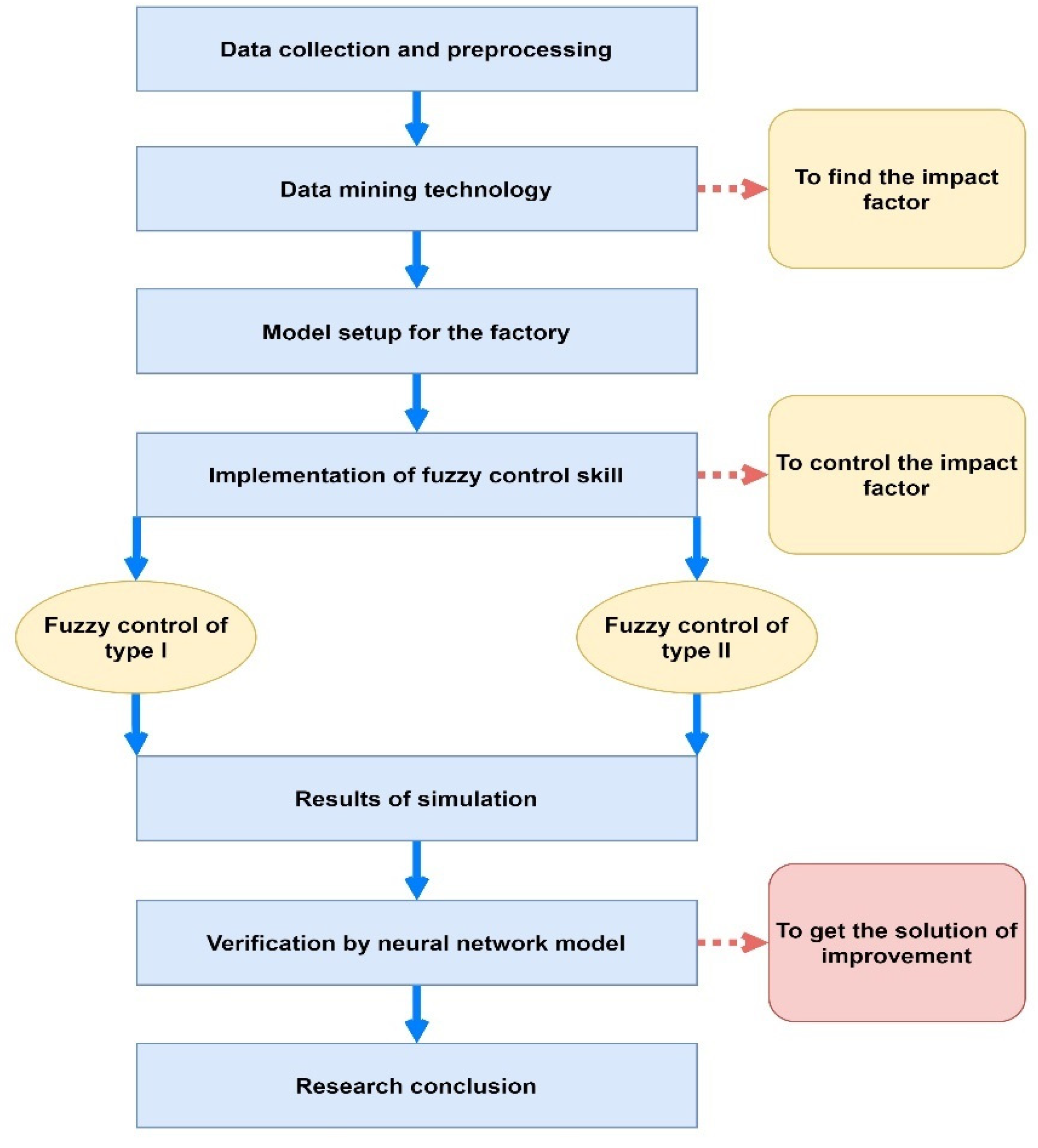
Regarding the proposed hybrid model, there are seven core steps addressed, including data collection and preprocessing, data mining technique, manufacturing model establishment, fuzzy control technology, effect comparison of simulation, effect verification of NN, and drawing conclusions. In detail, the first step of the proposed hybrid model is the data stage, including data collection and data preprocessing. Next, use data mining techniques to find out the important factors that affect the yield rate. The third step is to build a suitable model for the factory manufacturing process and use this mathematical model to apply radiant heat in a vacuum to imitate the structure of a physical factory. The following step accordingly uses the fuzzy control technique in order to control the found factors. With the comparison benefits, this study uses two types of fuzzy control methods and compares their experimental effects to see which structure is more ideal and suitable. The two types are presented as follows: (1) Type I: Uses fuzzy control to control PID in order to automatically adjust the three key parameters of Kp, Ki, and Kd to generate current (u) and to handle the controlled object to produce heat. (2) Type II: Uses the three key parameters of Kp, Ki, and Kd generated by the PID control in the previous method (1), and concurrently add the ΔKp, ΔKi, and ΔKd generated by the fuzzy control of the PID to produce current u; the mathematical equation for current is u = Kp + ΔKp + Ki + ΔKi + Kd + ΔKd. The electric current is generated by the thermal energy generated by the controlled body. Accordingly, the fifth step is to make the effect comparisons after implementing software simulation for the fuzzy control method. In the sixth step, we use the NN model to verify whether the effect of fuzzy control has reached the expected improvement goal. Finally, we confirm the empirical results with a meaningful conclusion. Figure 6 displays the flow chart for the seven steps in this research architecture. Importantly, algorithms of the proposed hybrid model in four stages are implemented stage-by-stage to show its detailed procedure in the following four sections, mainly including data preprocessing, modeling a mathematical model of a factory, modeling a fuzzy control model, and simulation verification. Initially, in the first stage, there are four main procedures (data collection, data classification, data exploration and calculation, and data analysis) described in the following four subsections.

3.1.1. Data Features and Data Collection from Factory with Its Equipment

This research is first aimed at the process of acquiring peripheral equipment for the coating machine from an optoelectronic company. The peripheral equipment process is presented in the following three key sub-processes: (1) After the ice water host is cooled, the ice water is stored in the water tower of this process, and then it is pumped into the filter by the ice water pump so that after the ice water is filtered, it can reenter the host for the cooling water cycle. (2) After cooling, the temperature is regulated by a plate heat exchanger, and then it is used for coating equipment, so that the cooling cycle continues repeatedly. (3) The main function of the cooling water tower is to prevent the host of ice water from overheating and causing a shutdown; in particular, the main function of the softening system of water is to control the water quality so as not to let the water quality deteriorate or let scale accumulate, causing the cooling water pipes to be blocked. Accordingly, the factory data is mainly focused on the three core features, including cooling water inlet pressure, cooling water return pressure, and cooling water temperature. However, in the processing system of a factory, the three features play an extremely important and interesting role. That is, if the pressure and temperature for the cooling water are insufficient, the components with heat sources in the equipment will be damaged due to overheating, and in severe cases, the equipment will be broken and the functions of evaporation will be stopped. Thus, the conditions for the three features must be given a high priority and be specifically considered. Moreover, the 12 attributes of the process equipment identified by professional experts include production month, job number, product type, equipment code, substrate size, yield rate, cause of failure, yield distribution, substrate temperature, cavity temperature, and the two spot positions of medicinal materials, SiO2 and Ta2O5. The data collection of the 12 attributes is conducted, and the instances collected from the 12 attributes of product lines can be used for further statistics and analysis purposes from the perspective of industrial data. Especially in this era of data explosion, it is important to quickly organize the data into usable information. When data is sorted and analyzed, it can become an important information asset, and after the evolution process, it can become key knowledge in the factory. Thus, we can benefit from the four knowledge forming processes of data collection → useful information → critical knowledge → higher wisdom.

3.1.2. Data Preprocessing for Further Automatic Classification

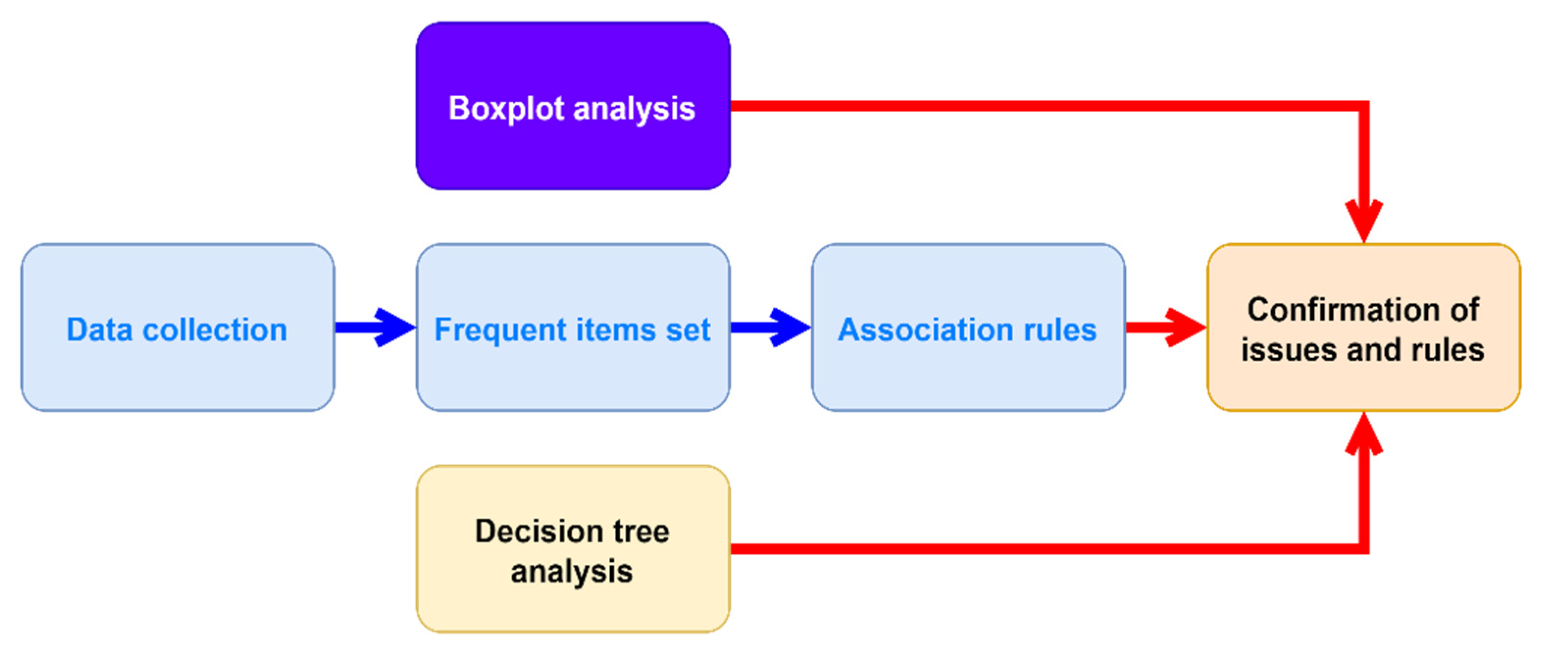
It is necessary that the data of products collected, including 50G, 100G, 800G, and CWDM, from the factory be first preprocessed and classified for further speeding the automatic classification in order to advantage the effective analysis of big data mining; thus, the decisional attributes of products are classified into the three classes of good, normal, and bad. Figure 7 shows the flow chart for well-used data mining techniques in this study. From Figure 7, it is seen that after collecting the industrial data, there are three effective analysis techniques: box-and-whisker analysis, association rule, and decision tree, for data mining functions in order to figure out and confirm the problem faced and the decisional rules generated from the decision tree. Specifically, we can accordingly create association rules after extracting frequent item sets.

3.2. Modeling a Mathematical Model

In order to make the simulation more realistic and practical based on the industrial data of the case study, this research will imitate a mathematical model similar to the on-site environment of a factory. For the detailed process, we first refer to the related literature for radiation heat transfer in a vacuum state, and we apply the equation of radiation heat transfer to establish a mathematical model of simulation for an evaporation factory. There are a lot of parameters used in the peripheral equipment of the factory; especially, five key elements, such as temperature, vacuum degree, electron gun, ion source, and cooling water, are identified as core factors for evaporation equipment. Among them, temperature is the most important factor, so we used temperature as the main consideration to establish a mathematical model of simulation and set up a set of effective fuzzy control methods to improve the yield rate of the factory production process. The mathematical model of simulation can be used as a future reference to increase the processes in factories. Next, five subsections are addressed for the proposed model with a variety of experiments, as follows:

3.2.1. Establish a Mathematical Model with Temperature Changes

When the testing object is placed in the heated test chamber with temperature T e (in a vacuum state at this time), its temperature T will gradually rise due to the absorption of radiant heat from the wall of the test chamber. According to the principle of energy conservation, the change of T in the heating process can be expressed and formatted as Equations (11) and (12) [42,43] as a differential equation:
M C d T = ε A σ T e 4 T 4 d t
or
q R = M C d T d t = ε A σ ( T e 4 T 4 )
where q R is the radiative heat transfer rate, and the rate of change of the temperature T of the test substrate with time t. The Y R is expressed and defined in an Equation (13) as follows:
Y R = d T d t = ε A σ M C ( T e 4 T 4 )
In the above equation, q is energy, and R is radiant heat. The reflected part is q R , σ is a proportional constant, also known as Stephen—Boltzmann constant, the true value is 5.67 × 10 8   W / m 2 K 4 , A is the thermal radiation on the surface area of the body, and T is the temperature of the heat radiator (in K), also known as “Boltzmann’s law of thermal radiation”.
To derive the above equations related to the experiments, the following parameters are used: (1) the mass of the testing object M = unit (in g), (2) the specific heat of the testing object C = degrees in unit (J/kg), (3) the surface area for the testing object A = unit cm2, (4) the emissivity ε of the surface for the testing object, (5) the temperature Te (K) of the heating test chamber, (6) the temperature T(K) of the testing object, and (7) the time t.

3.2.2. Building a Fuzzy Control Method

The substrate processing in the evaporation chamber is in a vacuum environment, which has two sets of heaters. One is the substrate heater; it is easy to control the temperature, and thus the temperature is relatively stable because the heater area is relatively small. The other is the cavity heater; it is relatively difficult to control the temperature stably because of its large area and the interference of two sets of high-temperature interference sources. Thus, this study uses the method of fuzzy control in order to effectively control the cavity heater, minimize the influence of interference sources, and adjust the temperature difference to be close to the substrate temperature so that the yield rate of production output can be effectively improved. Given the above reasons, there are three experiments addressing the substrate, chamber, and cavity wall for inducing dynamic equation derivation in the following descriptions of three subsections.

3.2.3. Dynamic Equation Derivation for Substrate Experiments

This study further analyzes the heat conduction system of vacuum coating. According to the theory of heat conduction, there are three types: conduction heat, convection heat, and radiation heat. In a vacuum environment, radiation heat transfer is the main method used. Therefore, this study focuses on the dynamic equation of thermal radiation and thermal conduction.
Furthermore, the effects of the cavity wall, the exchange of the two electron guns, and the radiation temperature of the cavity are considered based on the dynamic equation of the substrate temperature, as shown in Equations (14) and (15); where u is the substrate heating controller, with the mass M 1 , specific heat C1 of the substrate, surface area A 1 of the substrate, surface emissivity ε of the substrate, temperature T 1 of the substrate, and temperature T 2 of the cavity.
e = T 2 T 1
d T 1 d t = ε A 1 σ M 1 C 1 T W 4 T 1 4 + ε A 1 σ M 1 C 1 T e 1 4 T 1 4 + ε A 1 σ M 1 C 1 T e 2 4 T 1 4 + ε A 1 σ M 1 C 1 T 2 4 T 1 4 + u

3.2.4. Dynamic Equation Derivation for Chamber Experiments

Similar to the previous method, all the influences on some key substance materials, including the cavity wall, the two electron guns for the heater, and the radiation temperature of the substrate, are concurrently considered by the chamber dynamic equation, which is shown in Equation (16); where u 1 is the infrared (or IR) lamp heating controller, the mass of the cavity M 2 , specific heat C 2 of the cavity, surface area A 2 of the cavity, surface emissivity ε of the cavity, temperature T 2 of the cavity, and temperature T 1 of the substrate.
The dynamic equation for chamber temperature change is then formatted as follows:
d T 2 d t = ε A 2 σ M 2 C 2 T W 4 T 2 4 + ε A 2 σ M 2 C 2 T e 1 4 T 2 4 + ε A 2 σ M 2 C 2 T e 2 4 T 2 4 + ε A 2 σ M 2 C 2 T 1 4 T 2 4 + u 1

3.2.5. Dynamic Equation Derivation for Cavity Wall Experiments

Similarly, the temperature influence of the cavity and room temperature are also considered in the dynamic equation of the cavity wall, which is shown in Equation (17):
d T W d t = ε A 3 σ M 3 C 3 T 2 4 T W 4 ε A 4 σ M 4 C 4 T W T P
where M 3 is the mass of the cavity wall, the specific heat C 3 of the cavity wall, the surface area A 3 of the cavity wall, the surface emissivity ε of the cavity wall, the temperature T 2 of the cavity body, the temperature T W of the cavity wall, and the normal temperature T P of the indoor environment.

3.3. Research Method and Inference of Fuzzy Control PID

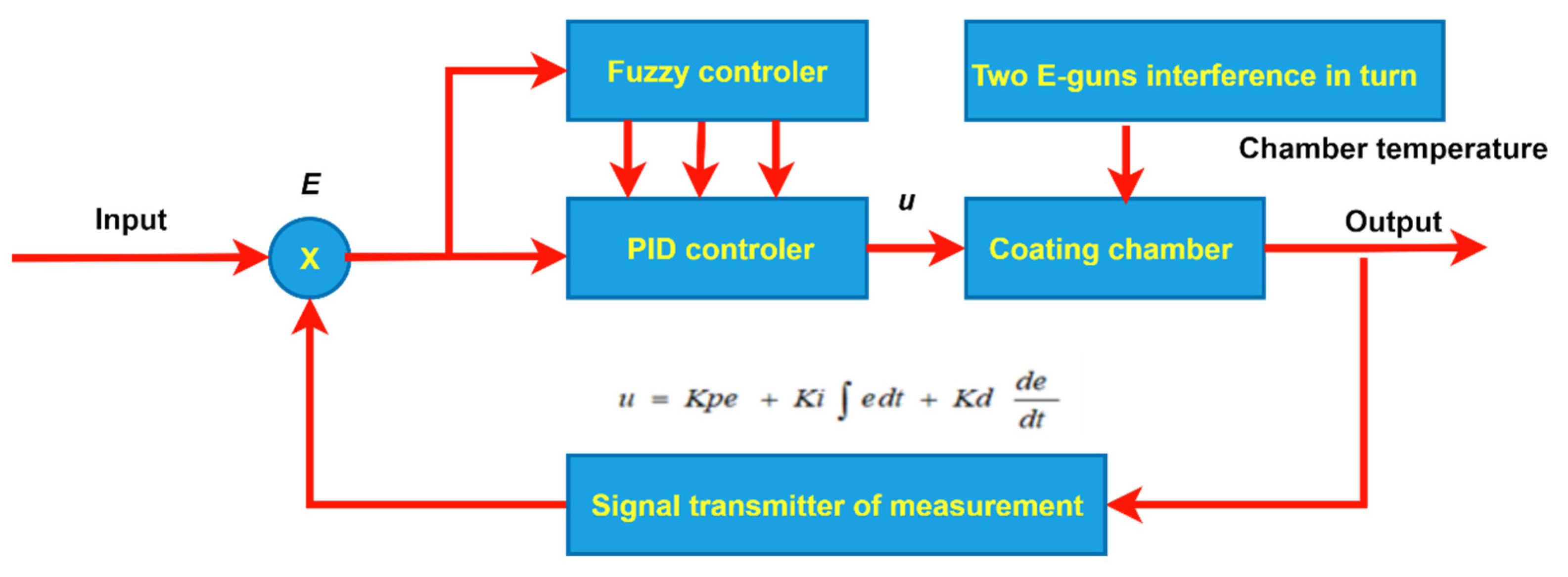
PID controllers are popular and advantageous in general factories. Importantly, a PID controller is needed when the water pressure or temperature need to be controlled at a fixed constant value. However, there are two serious flaws in the PID controller for controlling some conditions about temperature, as follows: (1) Internal interference determinants. The traditional PID controller is always used in the manufacturing factory, and its disadvantage is that the parametric conditions of the controller have not been corrected due to no use for too long. The parametric conditions may have some serious problems, such as the varying condition of the heating body, the aging of the temperature sensor, the declining of the power of the heater, and the varying space for the heating body. These problems lead to the parametric conditions being inaccurate, resulting in ineffective communication for the controller, and more seriously, damage and decrease the yield rate of the factory. Thus, these PID parameters must be adjusted appropriately and in a timely manner in order to control the temperature or other features accurately. (2) External interference sources: In addition, some external cases exist in the problem of an interference source, such as the different power outputs of two electron guns used to alternately interfere, or the heat interfering ion source, etc., which also results in inaccurate temperature control. Interestingly, using the fuzzy control method to continuously correct the parametric conditions of a PID controller is a novel industrial application that can solve these traditional problems. Based on this trigger, this study motivates the use of two types of different fuzzy control PIDs for the above issues faced by the optical filter industry and provides the rationale for proposing the hybrid model. Figure 8 first shows the processing environment for proposing Type I of fuzzy control PID. It is noted that the universal value’s intervals for the input and output variables of the fuzzy controller are obtained from industry experts’ recommendations for the two types (Type I for Simulation 1 and Type II for Simulation 2) used in this study.

3.3.1. Type I of Fuzzy Control PID with Its Research Simulation 1

In the Type I fuzzy control PID, it has a main processing flow in that it first adopts a fuzzy controller and receives the signal source of input e. After implementing the fuzzification with fuzzy rules and using fuzzy inference to make defuzzification, three kinds of output, Kp, Ki, and Kd [44], are produced, respectively. Figure 9 shows an architecture diagram of the fuzzy control PID [45]; it can be set for the input temperature starting at 25 degrees, and the maximum temperature is set at 175 degrees. Then, the fuzzy rules of fuzzy control are based on creating the three parameters Kp, Ki, and Kd and generating current u to the heater and heat the coating cavity; however, because of the high temperature of the two sets of electron guns, the output has the error of comparison on the cavity temperature feedback and is continuously adjusted to the set value of 175 degrees for finally reaching the effect of steady-state average temperature. Figure 10 shows the output and input diagram of the fuzzy control, which is the e (error value) of the set temperature for each input. After executing the fuzzy rules of fuzzy control, three adjusted parameters of Kp, Ki, and Kd are outputted and transmitted to u (current), and then continuously adjust the e value to the approximate value.
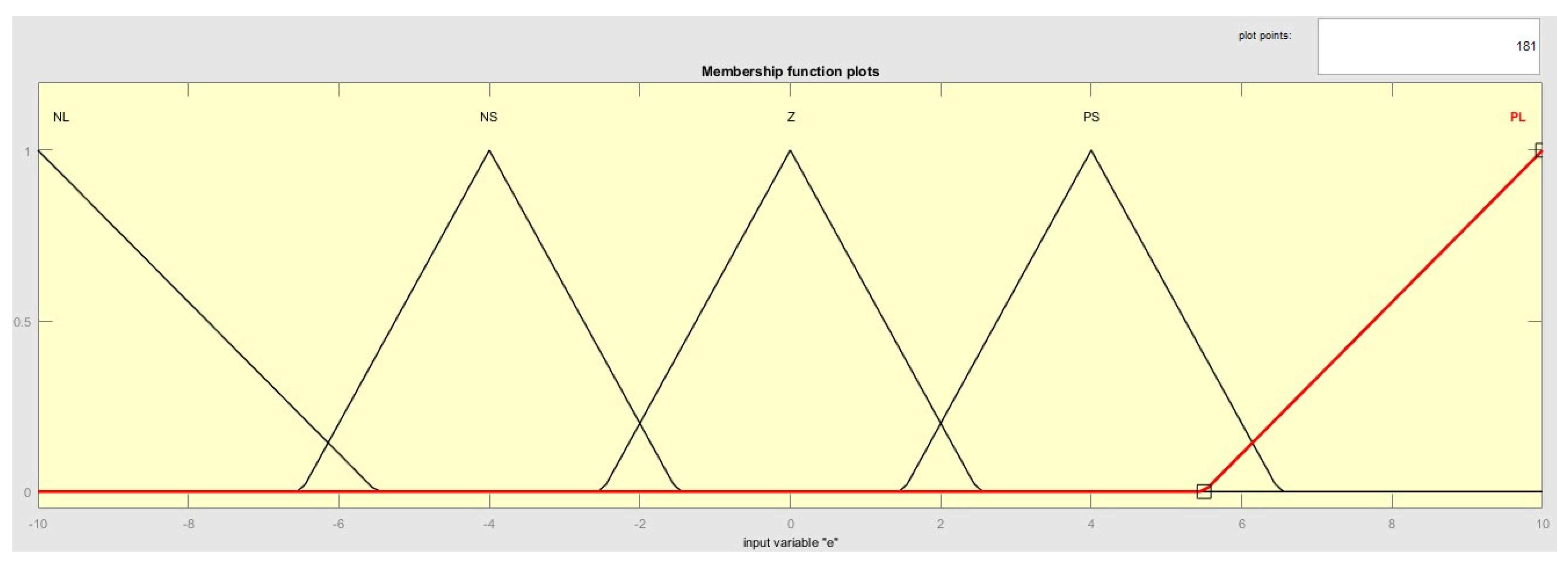
To further help understand the process of the Type I fuzzy control PID, there are four core directions addressed as follows: (1) Figure 11 presents the membership function for the input e of fuzzy control. From Figure 11, it is shown that the e value set for an input temperature and then its related membership functions have the following four situations: range of the NL (negative & large) is (−20~−5.5), range of the NS (negative & small) is (−6.5~−1.5), range of the ZE (zero) is (−2.5~2.5), range of the PS (positive & small) is (1.5~6.5), and range of the PL (positive & large) is (5.5~20.0). (2) Next, it is also shown that the input Kp value set for an output Kp is highlighted, and its related membership functions also have the following four situations: range of the NL is (−20.0~−5.0), range of the NS is (−7.0~−1.0), range of the ZE is (−2.0~2.0), range of the PS is (1.0~7.0), and range of the PL is (5.0~20.0). (3) In addition, for the input Ki of fuzzy control, there is a set output Ki highlighted, and its related membership functions also have the following four cases: range of the NL is (−15.0~−5.0), range of the NS is (−7.0~−1.0), range of the Z is (−2.0~2.0), range of the PS is (1.0~7.0), and range of the PL is (5.0~15.0). (4) Finally, the set input Kd of fuzzy control on an output Kd is highlighted, and its related membership functions are the same as the output Ki in the following four cases: range of the NL is also (−15.0~−5.0), range of the NS is also (−7.0~−1.0), range of the ZE is also (−2.0~2.0), range of the PS is also (1.0~7.0), and range of the PL is also (5.0~15.0).

3.3.2. Fuzzy Rules-Based System for PID

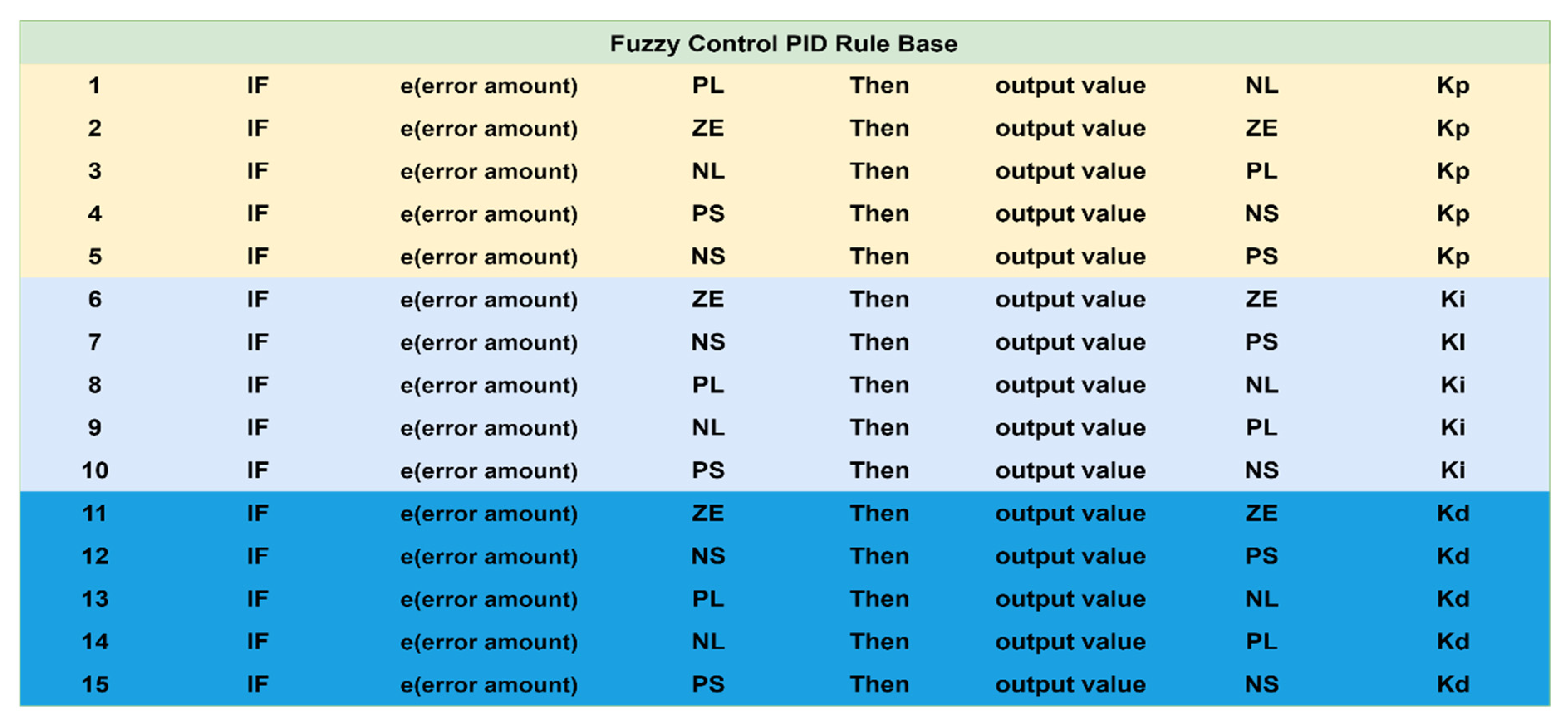
The rule base for processing the fuzzy control PID is addressed in a single input error value e. After implementing the fuzzy rules, a single output is generated: the three adjusted values of Kp, Ki, and Kd. First, the fuzzy rules base uses the input e value; that is, the e is entered into the rule base in order to adjust the PID parameters by matching the temperature set, and the current u generated accordingly flows into the cavity and then heats it. Next, the output value of temperature is compared with the value preset, and the temperature is constantly corrected and adjusted to make an approximate result of the temperature between the value preset and the output value achieved. Among them, the output value for the three parameters, Kp, Ki, and Kd, has been classified into meaningful semantic values of fuzzy; thus, there are three semantic situations productively determined by Simulink simulation results in this study. (1) The input e value has been identified as five kinds of semantic values of input, PL, ZE, NL, NS, and PS, for the Kp, which are used to generate the output Kp value by identifying the changing quantity for the five semantic values of output, NL, ZE, PL, NS, and PS. (2) The e value for the Ki value also has five variations of semantic values of input, ZE, NS, PL, NL, and PS, used to generate the changing quantity for the Ki value with five semantic values of output, ZE, PS, NL, PL, and NS. (3) The e value for the Kd value also has five variations of input, which are ZE, NS, PL, NL, and PS, used to generate the changing quantity for the Kd value with five semantic values of output, ZE, PS, NL, PL, and NS. Figure 12 shows the practical decision rules of the fuzzy-rules base; from Figure 12, we know that there are 15 rules in the fuzzy-rules base under the fuzzy control PID. In processing the implementation, when the set temperature e value is input, it first goes throughout the 15 fuzzy rules bases to adjust the values of the three output parameters Kp, Ki, and Kd, controls the output current u to feedback, and compares with e until it approaches the approximate value.
Next, we accordingly use Simulink simulation to design the four core control situations to implement the process of fuzzy control PID as follows:
(1)
For Equation (15): Uses the substrate of the PID control to derive the circuit diagram according to Equation (15) for the substrate experiment. In particular, the PID control allows the substrate to reach a stable temperature in a short time.
(2)
For Equation (16): Uses the chamber of PID control, and the circuit diagram is derived from Equation (16) for the chamber experiment; its temperature is set at 175 degrees plus 25 degrees at room temperature, two sets of interference sources of electron guns are added to switch alternately, and the cavity temperature is affected by the interference sources, making the temperature of PID control unsatisfactory. If we want to have a good control effect, constant adjustment of the current u of the output is needed to control the temperature by the PID.
(3)
For fuzzy-rules base: Uses the fuzzy control, according to Section 3.3.1, the concepts of fuzzy control and the fuzzy rules base in Figure 12, to adjust the three parameter variations of output to control the influence of the two sets of interference sources by the PID so that the temperature can be controlled close to ideal.
(4)
For Equation (17): Uses the circuit diagram derived from Equation (17) for the cavity wall experiment, and it will be affected by the evaporation coefficient at room temperature because the cavity wall is made of stainless steel which has the property of high thermal conductivity.

3.3.3. Type II of Fuzzy Control PID with Its Research Simulation 2

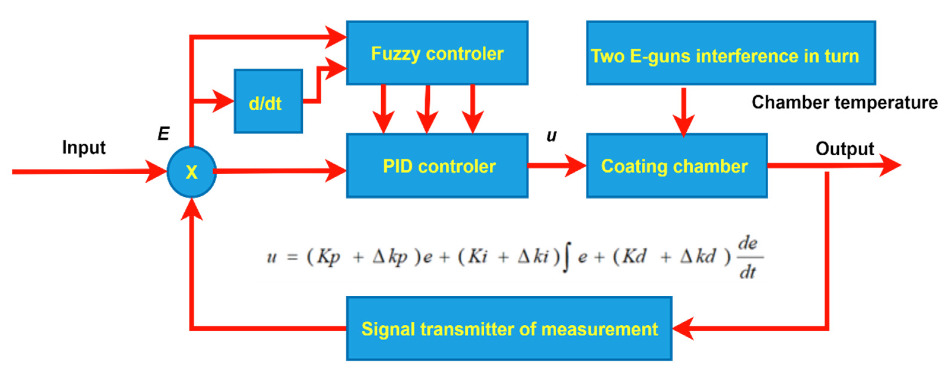
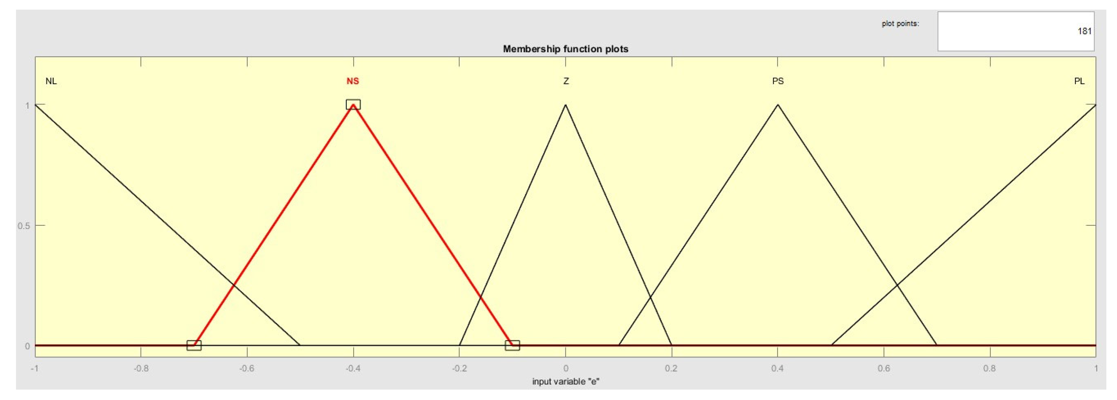
The second method of fuzzy control PID in this study is to mainly use the fuzzy controller to receive the input signal source of e (error) and d/dt (differentiator); after conducting the fuzzification and fuzzy-rules base and concurrently performing fuzzy inference to defuzzification, three kinds of output are obtained, including ΔKp, ΔKi, and ΔKd. Figure 13 shows the structure of the fuzzy PID algorithm [46,47], which is the result of fine-tuning ΔKp, ΔKi, and ΔKd for the fuzzy control after PID adjustment is applied. In implementing this Type II method, after tuning the PID controller, the variation of the temperature difference between the two sets of electron guns under high-temperature alternating interference has been greatly reduced. All the Kp, Ki, and Kd of PID plus the output ΔKp, ΔKi, and ΔKd of fuzzy control, respectively, are added to generate a current u transferring to the heater, which can provide feedback for error comparison of temperature between the heating cavity and the coating cavity after tuning continuous adjustment to measuring up the preset value of 175 degrees in order to achieve the effect of steady-state average temperature. Figure 14 presents the results for the input and output of the fuzzy control with the fine-tuning ΔKp, ΔKi, and ΔKd. From Figure 14, the input values of e and d/dt for the set temperature are determined, and the three outputs of ΔKp, ΔKi, and ΔKd are identified after tuning the fuzzy rules; afterwards, the three adjusted parameters are transmitted to u (current), and repeatedly, in this way, the e value is continuously adjusted to an approximate value. Similar to the previous method of Type I, there are five main directions for the e and d/dt addressed in the following explanations. (1) Figure 15 shows a membership function of fuzzy control for the input e of the set temperature. Based on the membership function of Figure 15, there are the following four situations: for the NL, its range is (−1.0~−0.5), its range is (−0.7~−0.1) for the NS, its range is (−0.2~0.2) for the ZE, its range is (0.1~0.7) for the PS, and its range is (0.5~1.0) for the PL. (2) Moreover, add the membership function of input d/dt and set the d/dt of the temperature for each input. Based on the membership function, there are also the following four situations: the range of the NL is (−1.0~−0.5), the range of the NS is (−0.7~−0.1), the range of the ZE is (−0.2~0.2), the range of the PS is (0.1~0.7), and the range of the PL is (0.5~1.0). (3) For the input ΔKp membership function and the setting ΔKp for each output, there are the following four situations: its range of the NL is (−2.0~−0.5), its range of the NS is (−0.7~−0.1), its range of the ZE is (−0.2~0.2), its range of the PS is (0.1~0.7), and its range of the PL is (0.5~2.0). (4) For the input ΔKi membership function and the setting ΔKi for each output, there are the following four situations: the range of the NL is (−1.5~−0.5), the range of the NS is (−0.7~−0.1), the range of the ZE is (−0.2~0.2), the range of the PS is (0.1~0.7), and the range of the PL is (0.5~1.5). (5) Finally, for the input ΔKd membership function and the setting ΔKd for each output, there are also the following four situations: the range of the NL is (−1.5~−0.5), the range of the NS is (−0.6~−0.01), the range of the ZE is (−0.05~0.05), the range of the PS is (0.01~0.6), and the range of the PL is (0.5~1.5).

3.3.4. PID + Kp, Ki, and Kd of Fuzzy-Rules Base

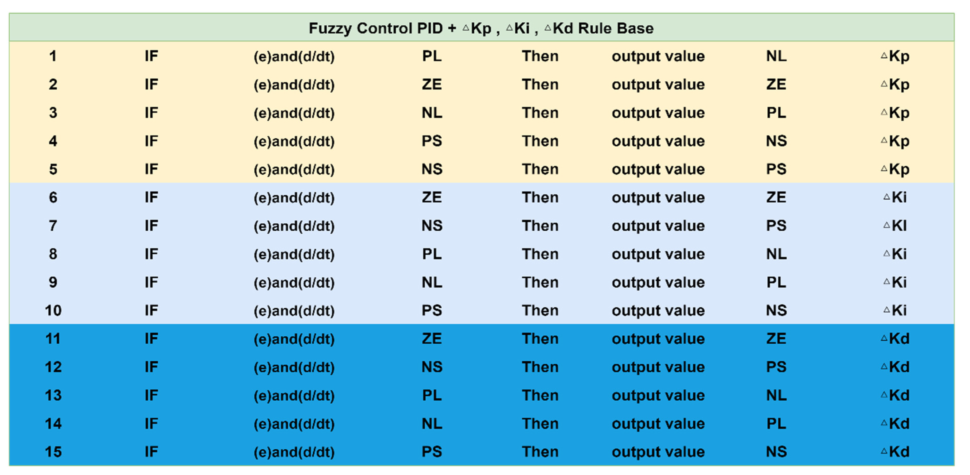
The rules used in this study in processing the fuzzy PID control have multiple input values, such as e value and d/dt (d/dt is an operational expression; d is not a differential but refers to a very small amount of change; d/dt differentiates with respect to t). After tuning the fuzzy rules, the single output is created and addressed in the adjustment values of three parameters, ΔKp, ΔKi, and ΔKd. After implementing the PID to control the temperature, add the ΔKp, ΔKi, and ΔKd of the fuzzy control PID, and then through the fuzzy-rules base, the input e value and d/dt enter the outputs, ΔKp, ΔKi, and ΔKd plus PID, of the fuzzy control for the set temperature; the generated current u is passed to the cavity for heating, and then the generated temperature is compared with the preset value. Accordingly, the temperature is continuously adjusted to produce a similar result for the difference between the set value and the output value obtained. Among them, the three output values, ΔKp, ΔKi, and ΔKd, have their fuzzy semantic values, respectively. The input of e value and d/dt for the ΔKp value has five kinds of semantic values, including PL, ZE, NL, PS, and NS, and it is used to generate the output value of the ΔKp with five fuzzy semantic values: NL, ZE, PL, ZE, and ZE. Likewise, the input e value and d/dt for the ΔKi value also have 5 kinds of fuzzy semantic values, ZE, NS, PL, NL, and PS, used to generate the output ΔKi for five semantic values of all zeros, i.e., ZE, ZE, ZE, ZE, and ZE. Similarly, the input e value and d/dt for the ΔKd value have five fuzzy semantic values, ZE, NS, PL, NL, and PS, used to generate the output value of ΔKd with five fuzzy semantic values, ZE, ZE, PS, NS, and ZE. Figure 16 shows the fuzzy rule base for the fuzzy control PID + ΔKp, ΔKi, and ΔKd. From Figure 16, there are 15 fuzzy decision rules defined. In implementing the process of Type II, it first goes through the 15 fuzzy rules after setting the temperature of input e and d/dt and then adjusts the output values of the three parameters, ΔKp, ΔKi, and ΔKd, to control the output current in the way of feedback until it reaches an approximate value in continuous adjustment for e. Afterwards, according to the fuzzy control and the fuzzy rules, we constantly adjust the output variations of parameters by the PID to effectively control the influence of the two sets of interference sources so that the temperature can be controlled close to the idealized effect.

3.4. Simulation Verification of an Intelligent NNs Model

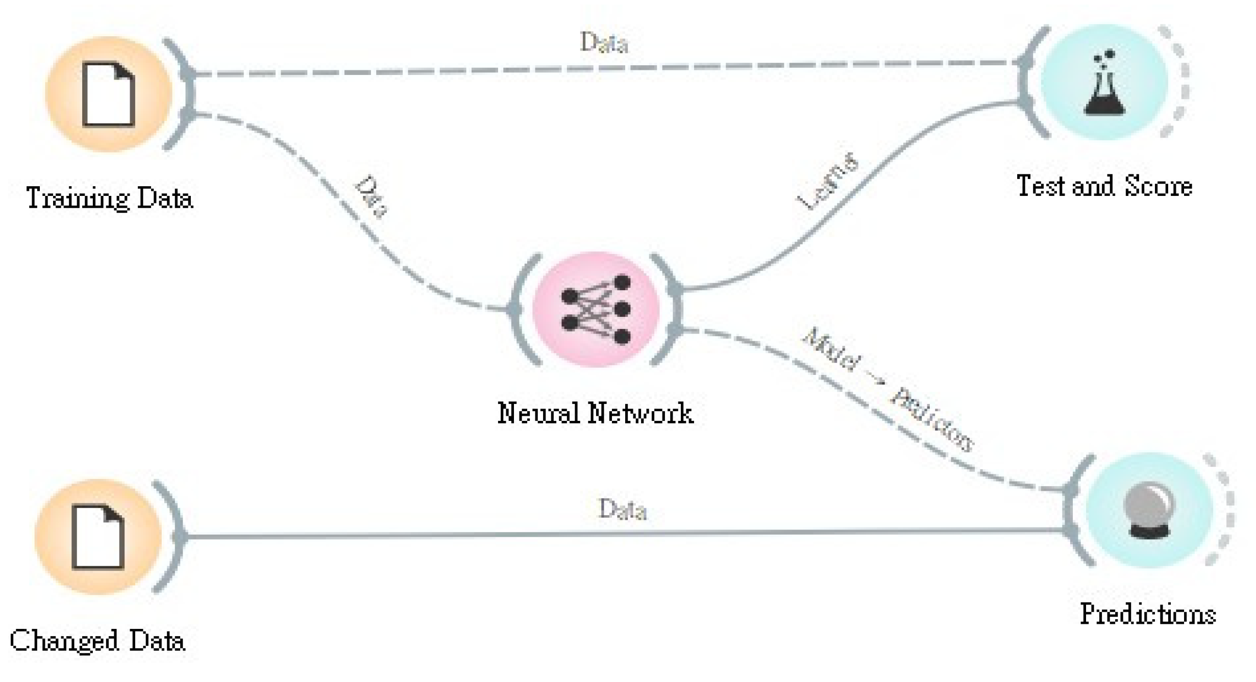
Figure 17 shows a structural diagram for processing a NN model. As shown in Figure 17, after collecting the industry data, the data are divided into two types: training and testing sets. The data contain the parameter values set and controlled by the peripheral control equipment and the evaporation machine equipment of the factory, respectively. We use the original conditions to establish a learning NN model through the training data. Then, we introduce the testing data into the learning process, set the neurons in the hidden layer of the NN, and choose Tanh(·) as the output activation function [48]; the Tanh function is also called the hyperbolic tangent function, which is proposed to solve the mean value problem on the basis of the Sigmoid function [49]. The range of values for the function is [−1, 1], and the corresponding average value of the output is 0. Tanh function will have a good effect when the characteristics are significantly different. The solver is set to use the stochastic gradient descent (SGD) method [50]; its advantage is that for large data sets, and the training speed is fast. A batch is randomly selected from the training set samples to calculate the gradient once, and the model parameters are updated once. The maximum number of iterations is selected to be 50 times. The testing results, testing scores, and predicted results can be obtained in a short period of time. It is one of the most useful and fast neural algorithms, designed to predict this kind of big data structure.
Applied to the practical cases of this study, the NN has two sets of input values, the training data and the testing data; after implementing the neural algorithm, two sets of corresponding output values for the testing score and prediction result can be obtained, respectively. Thus, the data obtained by the PID tester are used as the input layer to input X = { r 1 , r 2 , …, r N }. The sampling time will be every Δ t seconds, the impedance value of the ith measurement is r(it) = r i , the impedance value from the 1st to the Nth will be used as the input layers 1~N neurons, calculate the network weight value through Equation (6), and then guide the input weight value to the output layer through Equation (5). A set of input X and output Y data will be obtained. Not every training instance achieves the ideal network weight value immediately; thus, it is necessary to continuously correct the weight of each connection, and the weight value is connected to the neurons of the hidden layer and the output layer. Therefore, this study corrects the weight value in the way of supervised learning, supplemented by the form of BPNN, to correct the weight of the error function E in the form of Equation (7). Afterwards, we calculate in the hidden layer, and then calculate the calculated data with the Equation (8) and multiply the weight w j i n of the hidden layer and the output layer. Accordingly, the output layer summarizes the data, and the output layer compares the result with the target value (i.e., whether there exists a PID phenomenon). If the calculated output does not meet the expected target value, it will be returned to the input layer, and then recalculate the weight value of the connection weight value in Equation (7) with the hidden layer; repeat Equation (5) to calculate the output value of the hidden layer and the output layer until we get what we want: knowing whether there exists a PID phenomenon.
In addition, it is necessary to eliminate the data that may cause training errors in the input data and use other input data to supplement it. After finishing the supplement, re-enter the data into the input layer and calculate the output value for the input layer and hidden layer again. Finally, other validation data is fed into this modified and trained NN model [51]. Therefore, the construction of a NN model in this study is divided into three stages, namely training, verification, and testing, described separately. (1) Training: After the input data and structure size are determined in the training phase, the weights are adjusted; the training phase must provide enough data T R for the learning phase of the NN model. (2) Verification: Provide part of the data T V in the verification phase to verify whether the parameters and architecture of the training phase are appropriate, and select the most suitable model from them as the best architecture of the NN model used in the testing phase. (3) Testing: The testing phase mainly uses testing data T T to test whether the trained and verified NN model can meet the practical industry data application.

4. Data Analysis and Demonstration Results

After implementing the real-life case study, this section mainly describes the research results and evidence of effectiveness in three parts. First, we collect the practical data and, accordingly, use the analytical techniques. Second, we find out the relevance of the cause of the defect rate and use the fuzzy control PID to formulate fuzzy rules and make a comprehensive analysis [52]. Third, we use the Simulink simulation package to simulate the effect of fuzzy control with its experimental results. Thus, we have five sections to address the above processing scheme with results, including analysis results of data mining techniques, analysis results of Simulation 1 using fuzzy control, analysis results of Simulation 2 using fuzzy control, summary analysis of fuzzy control research, and verification results of NNs, respectively.

4.1. Analysis Results of Data Mining Techniques

We need to first define and describe the yield rate of the case study. Figure 18 shows the distribution of products for the yield rate in this case. From Figure 18, it is clear that we have defined three classes of products to distinguish the yield rate: 60% or more is good, 30%–60% is normal, and 0%–30% is bad. Interestingly, the bad rate is unacceptable.
Accordingly, based on actual features to analyze the industrial data from an optoelectronic company, Table 1 shows the partial data collected from factory affairs and equipment, and Table 2 shows the integrated partial data classified into three classes with sorting in decisional attribute (i.e., test result) for more convenient experimental operation and use. The three classes are good, normal, and bad. (Note the following abbreviations are defined for these terms: production month (P.M.), job number (J.N.), product code (P.C.), equipment code (E.C.), substrate size (S.S.), yield rate (Y.R.), cause of failure (C.F.), yield distribution (Y.D.), substrate temperature (S.T.), and cavity temperature (C.T.), cooling water temperature (C.W.T.), inlet water pressure (I.W.P.), return water pressure (R.W.P.), temperature difference between the cavity and the substrate (T.D.), good (G), normal (N), and bad (B)).

4.1.1. Analysis Results of Box-and-Whisker Plot

After performing the analysis of the box-and-whisker plot, Table 3 lists its summary for the analytical experiment. From Table 3, we can obtain characteristic results of seven items by the box-and-whisker plot, including substrate temperature, cavity temperature, cooling water temperature, inlet water pressure, Ta2O5 spot position, SiO2 spot position, and the temperature difference between the cavity and the substrate. It is clear that no significant difference exists in the first six items; conversely, the temperature difference in the seventh item has a significant difference. Thus, the temperature difference between the cavity and the substrate is a key determinant that influences the yield rate. From the perspective of temperature difference, there are three fuzzy levels identified. (1) In particular, the correlation outcome between the yield rate and the temperature difference within 2 °C to 3 °C is very good; (2) the correlation is normal when the temperature difference is within 3 °C to 9 °C; and (3) it is not a good correlation if the temperature difference is above 4 °C to 13.5 °C. Therefore, based on the above experimental results, we have found an important fact: the larger the temperature difference, the lower the yield rate. Based on the above interesting fact, this research is aimed at controlling the temperature difference to being as small as possible. It is most likely that the yield rate of the products can be improved by improving the temperature difference. Furthermore, it is also clear that there are obvious differences in the distribution from the evidence of the box-and-whisker plot for the conditional temperature difference of the product equipment. Regarding the box-and-whisker plot in Table 3, there are three categories, good, ordinary, and bad, for the yield rate, which is also proved and determined by the cavity and the substrate. (1) In terms of temperature difference, the average temperature difference is about 2.37 degrees when the yield rate is good, and its distribution range is relatively low and concentrated. (2) The average temperature difference is about 6.12 degrees when the yield rate is normal, and its distribution range is relatively large. (3) When the inspection outcome is not good, the average temperature difference is about 9.25 degrees, and its distribution range is relatively larger and less concentrated when compared to the other two cases. Furthermore, from a distribution analysis of the box-and-whisker plot for the cooling water pressure, it is also clear that there are three categories, very good, ordinary, and bad, addressed and identified for the yield rate. (1) From the perspective of cooling water pressure, the yield rate is good when the average water pressure is about 3.46 kg, the water pressure range is from 3.3 kg to 3.8 kg, and it is implied to need stronger water pressure for “cooling” temperature. (2) The yield rate is normal when the average water pressure is 3.32 kg, the water pressure range is from 2.8 kg to 3.8 kg, and the water pressure tends to be at a “weak cooling” temperature. (3) The yield rate is bad when the average water pressure is about 3.2 kg, the water pressure range is from 2.8 kg to 3.6 kg, and the water pressure is also identified as a biased “weak cooling” temperature. Therefore, focusing on the above experimental results, there also exists a significant difference in the cooling water pressure, and when the cooling water pressure is stronger, the yield rate has a better outcome.

4.1.2. Analysis Results of Association Rule

After implementing the association rule, Table 4 shows its analytical results for the seven conditional attributes mentioned above. From Table 4, the results of seven featured attributes for the correlation with the one decisional attribute (i.e., the yield rate) can be observed. There are also seven features in the previous subsection, and the seventh item, the temperature difference between the cavity and the substrate, has a significant difference. There are four key points to address in the analytical results. (1) If the average temperature difference is within 2.3 degrees, the yield rate is very good; the yield rate is normal if the average temperature difference is within 6.1 degrees, and the yield rate will be bad if the average temperature difference is within 9.25 degrees. (2) The above results are the same as the results of the box-and-whisker method. Interestingly, we also have an important research finding: the greater the average temperature difference, the worse the yield rate. Thus, this study also needs to mainly control the average temperature difference close to the ideal value in order to improve the yield rate of products. (3) Afterwards, with the discretization of numerical items, we can obtain the 5 frequent items of high-density products when the number of intervals of equal-frequency discretization is set to 2, the number of itemsets is 2 when the minimum support is set at 3%, the support achieves 3.67% when the temperature difference between the cavity and the substrate is less than or equal to 6.75, and thus, the yield rate is very good. (4) Moreover, according to the analytical results of association rules, two decision rules are generated if the minimum support is set at 37.0% and the minimum reliability is set at 74.0%. This implied two important industry rule findings. Rule 1: The cooling water temperature is greater than 20.75 degrees if the inlet water pressure is less than 3.25 kg. Rule 2: The yield rate is bad when the temperature difference between the cavity and the substrate is greater than 6.75 degrees.

4.1.3. Analysis Results of Decision Tree

Subsequently, Table 5 shows the analytical summary for the decision tree technique. From Table 5, similar to the results of the first two methods, a total of seven features are also defined, and the seventh item, the temperature difference between the cavity and the substrate, has a significant difference in the yield rate. We also have four directions for determining the analytical results. (1) The yield rate is very good if the temperature difference is within 2 degrees, but it accounts for only 3.7%; the yield rate is normal if the temperature difference is within 2 degrees to 8.59 degrees, and its ratio has 40.10%; the yield rate is bad if the temperature difference is above 8.5 degrees to 17 degrees, and its ratio has 56.20%; therefore, the larger the temperature difference, the worse the yield rate. From the analysis results of the decision tree, similar to the previous two methods, this research is still moving towards the goal of controlling the temperature difference to make it close to the ideal value to improve the yield rate. (2) There are three classes for bad, normal, and good yield rates, which are executed for decisional rules, respectively. The first is the results of the decision tree analysis of the bad yield rate. There are 1008 items; among them, 567 items have a temperature difference greater than 8.5 degrees to 17 degrees, and 56.2% of them indicate that if the temperature difference is too large, the yield rate is obviously bad. (3) The second is the result of the decision tree analysis with the normal yield rate. There are 404 items defined with a temperature difference between less than 2 degrees and 8.5 degrees; there are 40.1% of them. It can be identified that if the temperature difference is within this range, the yield rate is normal. (4) The last are the results of the decision tree analysis with a good yield rate. There are 37 items with a temperature difference of less than 2 degrees, accounting for a total of 3.7%. It can also be defined that the temperature difference falls within this range, and then the yield rate is very good. Productively, through the above analysis results from the decision tree technique, it is identified that we should be committed to adjusting and controlling the temperature difference between the substrate and the cavity. If it can be controlled within 2 degrees, it will greatly help produce better products in the production process.

4.1.4. Analysis Results of Fuzzy Control

Regarding the fuzzy control analysis, Table 6 shows the parameters of the mathematical model for the case factory after performing fuzzy control. From Table 6, it means that these parameters are approximate practice data from the factory site, and they are brought into the simulation system constructed. In order to make the experimental results more simulated and realistic, the three most important factors include the substrate, cavity, and cavity wall. The parameters are set according to the setting values of the actual field.

4.2. Analysis Results of the Fuzzy Control PID Simulation Method 1

Following the previous section on using data mining techniques, we accordingly perform the fuzzy control PID simulation method. First, we show the PID control of the cavity for the original job site. Next, it is known that there are two electron guns: one is an electron gun with a larger change and a higher power, and the other is an electron gun with a smaller change and a lower power. The two electron guns operate alternately; the highest temperature is about 190 degrees; when another electron gun with a lower power is replaced, the temperature drops to about 160 degrees, and their temperature difference is about 30 degrees. However, because the power of the two electron guns in some processes is different, the temperature difference may vary even more, and the difference may be between 20 and 30 degrees; it is a key to note that this difference may cause poor yield rates. Moreover, because the heater area of the substrate for the optical coating machine is relatively small, it is easier to control the temperature. While the cavity area is larger, the IR heaters surround the four sides of the cavity. In particular, there are two electron guns alternately melting the powder, and a large voltage and a low current are used for melting the powder at high temperatures; the temperature can reach up to 1000 degrees or more, and thus, it is very difficult to control the temperature because of the huge factors of temperature variation. Importantly, the temperature control of the cavity is mainly emphasized in this study, and the way of using the fuzzy control method is to majorly control the nonlinear temperature in the cavity so as to achieve the effect that the temperature difference between the substrate and the cavity can be closer. Given the above problem from the original job site, this study makes an adjustment and improvement with the electron gun after the fuzzy control; the improvement includes one electron gun with a higher power and the other with a lower power. In particular, after the fuzzy control of PID in this experimental method, the higher-power electron gun is set to about 176 degrees, and the lower-power electron gun is set to about 174 degrees. Their temperature difference has a significant low range of only about 2 degrees, and productively, this excellent result can significantly increase the yield rate for the products of the case study.

4.3. Analysis Results of the Fuzzy Control PID Simulation Method 2

For the comparison benefits, we make another simulation method of the fuzzy control PID. This study has analyzed results of fine-tuning ΔKp, ΔKi, and ΔKd by the fuzzy control after PID adjustment; the adjustment has the one with the higher power of the electron gun and the other with the lower power. Therefore, the two electron guns operate alternately; when the first electron gun operates, the temperature rises to about 178 degrees at the beginning, and after about 100 s after the fuzzy control adjustment, the temperature slowly drops to about 177 degrees. Consequently, after about 500 s, the temperature is set to fit the target value of 175 degrees, and then the steady-state situation is reached. However, when the second electron gun is turned on, the temperature drops to 172 degrees, and then it can reach 174 degrees because of the adjustment made by the fuzzy control PID. Finally, the minimum temperature difference is reduced to about 1 degree, and it is proven that this method can make the temperature difference less, smoother, and better, thereby benefiting the yield rate. Interestingly, this method 2 significantly improves the yield rate of the case study factory.

4.4. Research Summary for the Analysis Results of the Fuzzy Control

Subsequently, we make a comparable study for the above methods. In the original method for the case study factory, the following descriptions are for the current status of the manufacturing process site. When the high-power electron gun is turned on, the temperature is above 190 degrees, and it will be pulled back to 177 degrees after the PID control. However, when the high-power electron gun is turned off and the low-power electron gun is turned on, the temperature drops to 162 degrees, and we compensate the temperature to 173 degrees through the PID control. In order to solve the above problem of large temperature differences, we have the following two methods: (1) Experimental method 1 of the fuzzy control research: For the experimental result of the fuzzy control PID, when the electron gun interference source input is after fuzzy control, the temperature is quickly adjusted to 176 degrees, but when the second electron gun is turned on, the temperature first drops and then pulls back to 174 degrees, so the temperature difference is about 2 degrees. (2) Experimental method 2 of the fuzzy control research: For the result of fine-tuning ΔKp, ΔKi, and ΔKd using the fuzzy control after the PID control, when the first electron gun is turned on, the temperature is about 178 degrees; importantly, after tuning the fuzzy control adjustment for about 100 s, the temperature slowly drops to about 177 degrees. Accordingly, after about 500 s, the temperature reaches the target value of 175 degrees, and then it reaches a good steady-state status. However, when the second electron gun is turned on, the temperature drops to 172 degrees, and after tuning the fuzzy control adjustment again, it reaches 174 degrees, which has a temperature difference of one degree. It seems to have a good outcome for the yield rate.

4.5. Verification Results of the NN Model Simulation

Subsequently, Figure 19 shows a graph for the verification results of performing the NN model. From Figure 19, the X-axis is the temperature difference in degrees, and the Y-axis is the yield rate in terms of percent. Moreover, Table 7 lists the detailed verification outcomes of the NN model. It can be determined that the total number of records is 700 after using the NN algorithms. From Table 7, the verification results show the following facts: The temperature differences are identified from 0, 1, 2, 3, 4, 5, 6, 7, 8, 9, 10, … to 20 degrees, and concurrently, their yield rates are achieved, corresponding to 98.57%, 98.57%, 92.85%, 85.71%, 74.28%, 71.4%, 59.71%, 57.14%, 54.28%, 47.14%, 42.85%, 31.42%, 22.8%, … to 0%, respectively. Interestingly, based on the above results, an important research finding is unearthed: it is the best choice for positively influencing the yield rate to effectively control the temperature difference between the temperatures of substrate and cavity within one degree, and it is a key industrial contribution for benefiting the case study factory to proactively identify its manufacturing processing with the benefit of better-quality products and productivity. Productively, the smaller the temperature difference, the better the yield rate. The new production process can significantly improve the stability and operation performance of the products compared to the original processing.
The equipment cost and time cost of the physical manufacturing process are both very high, and the product defect rate is also high, which will affect the company’s profitability and competitiveness. Before carrying out the physical manufacturing process, this study used fuzzy control technology to improve the temperature difference based on empirical data provided by professionals and used neural networks to verify the effect. Finally, a method to improve the yield rate was derived to ensure that manufacturing costs can be reduced and product quality can improve in the physical process in the future.
The results of this study show that before the problem is solved, when the difference between the substrate temperature and the cavity temperature is too large, the yield is not good. The results after improvement through two fuzzy control technologies, Types I and Types II, are as follows: (1) After improvement of Type I, after fuzzy control simulation and online correction PID, the average temperature difference can be controlled to about 2 degrees, but the shortcoming is that it cannot reach the target value of 175 degrees. (2) After improvement of Type II, after PID control, fuzzy control is added to fine-tune Kp, Ki, and Kd. After correction by fuzzy control online, the average temperature difference can be controlled by about 1 degree, and the correction speed is slow.

5. Conclusions and Future Research

This section has mainly made a conclusive summary with a subsequent direction for the issue of the yield rate in the optical filter industry, including three concerns about conclusions with research findings and contributions, a summary of important achievements, and the future prospects of this study.

5.1. Conclusions with Research Findings and Contributions

The research object of this study is focused on processing the optical filter of optical communication components, and the processing is an advanced optical precision process. Due to the rapid development of information technology, the transmission of the network is getting faster and faster, from early 2G communication to current 5G communication with continuing development, and the progress has moved towards the era of future 6G. Therefore, in the manufacturing process of products related to optical communication, to maintain their advantage of a high yield rate, the related processes become extremely important. Based on alleviating this concern, the relevant techniques used in this study have been improving in the optical filter industry for industrial value. Thus, this study makes good use of data mining techniques to deal with various classification problems and dig out some consequential research findings, and we chose an appropriate method for addressing a good industrial data analysis. Thus, this study has proposed a hybrid model with an important technical contribution from the perspective of industrial application. In the detailed processing for the proposed hybrid model, there are five key points highlighted. (1) This study uses the statistical analysis of yield rate distribution, association rules, and decision tree classifiers in order to find out the potential reasons for the defect rate of the products on the production process line and then to improve it. (2) In the use of data mining techniques, it has been found that the main reason for the defect rate is that the temperature difference between the substrate and the cavity during the product manufacturing process is too large, which causes reduced output. (3) In order to overcome the problem of excessive temperature difference, this study uses the tool of fuzzy control PID to dominate the varied changes of the three temperature parameters, Kp, Ki, and Kd, and then further change its output current u. (4) We further used Simulink simulation software to completely simulate the experimental results. By analyzing the results to explore the real cause of the problem, this problem is reduced and solved, and the yield rate is improved; thus, we have industrial applicability value based on the application’s context. (5) Finally, it is expected that the yield rate can be further improved, and by rapidly driving the production speed of 5G for 100G optical filters, the manufacturing cost can be further reduced, and the technology of the future optical communication industry can be improved.
Furthermore, there are eight points that summarize this study and the implemented experiments:
(1)
Motivation of the study: In response to the strong demand for optical filters after the market upgrade from 4G to 5G, a serious problem has emerged. However, because of the long manufacturing process, high manufacturing cost, low yield rate, and many influencing factors, the market faces short supply and cannot keep up with demand. Thus, the study is motivated by this interesting issue and provides an effective hybrid model to identify and improve the yield rate of optical filters for the communication industry and increase its production quantity while maximizing efficiency in order to meet market demand. Therefore, this study offers valuable industry experience in this important domain of the optical communication industry.
(2)
Data mining analysis methods used: This study uses three data mining analysis techniques, including the box-and-whisker method, the association rule method, and the decision tree method. After analyzing the experimental results, it is found that temperature is the key determinant influencing the output of products, and the main results are as follows: (a) Among the 1008 cases where temperature differences between the cavity and the substrate occurred, 567 cases were between 8.5 °C and above 17 °C; that is, 56.2% of the yield rate of products was bad. (b) There are 404 cases between 2 °C and 8.5 °C, and 40.1% of the yield rate is normal. (c) Only 37 cases have a temperature of less than 2 °C, and only 3.7% of the yield rate is good.
(3)
Important research finding: From the analysis results of data mining techniques, there is an important research finding; that is, it is found that the correlation between the yield rate of the process and the interference source of temperature has a significant influence on affecting the output rate of products and easily causes a high defective rate in bad situations.
(4)
Another research finding: From the empirical results, it is also found that when the temperature difference between the substrate and the cavity is too large, it is one of the main reasons for poor yield rate. This research finding can be further explored in subsequent research.
(5)
Types I and II of two fuzzy control techniques: In order to better control the temperature variation, this study uses two types (I and II) of fuzzy control techniques, and the results obtained are as follows: (a) The result of the Type I method can make the temperature difference between the cavity and the substrate controlled within two degrees; (b) the result of the Type II method can first control the temperature difference within about six degrees at the beginning; however, after continuous fuzzy control correction, it can be controlled with one degree close to the approximate value and ideal value and achieve the best situation for the yield rate of the case study factory.
(6)
One significant verification result: The verification result of the alternative research method is to consider and use the simulation function on the NN model with the following three research highlights: (a) it is verified that if the temperature difference is less than two degrees, the yield rate is good; (b) if the temperature difference is less than eight degrees, the yield rate is normal; and (c) if the temperature difference is greater than 10 degrees, the yield rate has a bad effect on the bottom line.
(7)
Poor performance for identifying temperature difference: After the important analysis of industry data from benefiting the data mining techniques, this study finds that the yield rate has an obvious poor performance when the temperature difference between the substrate and the cavity is too large. It is defined that the larger the temperature difference, the poorer the performance.
(8)
Valuable contribution for industry application: This study has important industrial application contributions; that is, the use of the fuzzy control PID technique [53] to better control temperature can significantly improve the yield rate and reduce manufacturing costs, direct labor costs, direct material consumption, etc. Concurrently, it can mass-produce high-precision optical filters, thereby quickly driving the technology era of 5G with high-speed network products such as the Internet of Things (IoT), unmanned autonomous driving, and AI. They have made it more stable and mature, thereby adding a small step to the applicable contribution for industry data of the Internet generation with a major development.

5.2. Summary of Important Achievements

The research object of this study is optical filters for 5G and optical coating; it is the main component of future optical communication, but it has some disadvantages in the manufacturing process, such as production difficulty, long time, high cost, and low yield rate. In order to solve these plights, this study has some important achievements and advantages: (a) This study employs big data mining technology to find out the potential cause of the yield rate problem and employs the fuzzy control technique to control the PID thermostat [47], further facilitating model simulation; (b) it continuously adjusts the interference from the interference source to improve the temperature difference with some strengths, such as the improved yield rate of processing optical filters. The filters can be produced quickly, manpower is reduced, time is shortened, and cost loss is reduced.
The reason for using fuzzy control technology to simulate and improve the temperature difference is because the manufacturing cost of the process is high and the manufacturing time is long, so it is challenging to conduct real experiments. Fuzzy PID controller is a control algorithm based on fuzzy logic, which combines the advantages of fuzzy control and PID control. Compared with traditional PID controllers, fuzzy PID controllers can better adapt to complex nonlinear systems and show better performance in terms of control effect and stability. The fuzzy PID controller uses the control parameter adjustment principle derived from the practice of empirical rules to define a fuzzy rule table; the fuzzy controller is used to instantly correct the parameters of the PID controller; on the basis of the traditional PID, the parameters KP, KI, and KD are each increased by one amount of change. Fuzzy PID has better performance than PID. In the future, we will move towards using the researched fuzzy controller to use a combination of software and hardware to bring it into the actual process to verify its effect.

5.3. Future Directions

Although this study uses big data mining technology to see the reasons for the defect rate of the production line and efficiently uses fuzzy control technology to improve the difference degrees of temperature, and the actual research output has conclusively achieved remarkable results, there is still room for improvement in several key areas: (1) In the future, actual experiments can be performed instead of using simulation methods, and then the two experimental results can be practically compared. (2) For the Simulink simulation, many parameter values can be further adjusted continuously, hoping to achieve the desired absolute goal. (3) It is also expected that the academic research results can be fully disclosed to companies in order to achieve the combination of both academic theory and industrial practice, which can greatly improve the production yield and make production more efficient. Thus, the technological development of this industry can be rapidly improved.

Author Contributions

Conceptualization, J.-R.C. and Y.-S.C.; Methodology, J.-R.C. and Y.-S.C.; Software, C.-Y.C.; Visualization, C.-Y.C., Y.-H.H. and M.Y.-J.L.; Writing—original draft, C.-Y.C.; Writing—review and editing, Y.-H.H., Y.-S.C., C.-J.L. and M.Y.-J.L. All authors have read and agreed to the published version of the manuscript.

Funding

This research was partially supported by the National Science and Technology Council of Taiwan for grant number 111-2221-E-167-036-MY2.

Institutional Review Board Statement

Not applicable.

Informed Consent Statement

Not applicable.

Data Availability Statement

No new data were created or analyzed in this study. Data sharing is not applicable to this article.

Conflicts of Interest

The authors declare no conflicts of interest.

References

  1. Haddi, S.B.; Zugari, A.; Zakriti, A.; Achraou, S. 5G narrow-band band-pass filter using parallel coupled lines and L-shaped resonator. In Proceedings of the 2020 International Symposium on Advanced Electrical and Communication Technologies (ISAECT), Marrakech, Morocco, 25–27 November 2020; pp. 1–4. [Google Scholar] [CrossRef]
  2. Dzogovic, B.; Van Do, T.; Santos, B.; Feng, B.; Jacot, N. Thunderbolt-3 backbone for augmented 5G network slicing in cloud-radio access networks. In Proceedings of the 2019 IEEE 2nd 5G World Forum (5GWF), Dresden, Germany, 30 September–2 October 2019; pp. 415–420. [Google Scholar] [CrossRef]
  3. Gladju, J.; Kamalam, B.S.; Kanagaraj, A. Applications of data mining and machine learning framework in aquaculture and fisheries: A review. Smart Agric. Technol. 2022, 2, 100061. [Google Scholar] [CrossRef]
  4. Guo, Y.; Zhang, W.; Qin, Q.; Chen, K.; Wei, Y. Intelligent manufacturing management system based on data mining in artificial intelligence energy-saving resources. Soft Comput. 2023, 27, 4061–4076. [Google Scholar] [CrossRef]
  5. Du, Y.; Yang, C.; Zhao, B.; Hu, C.; Zhang, H.; Yu, Z.; Gao, J.; Zhao, W.; Wang, H. Optimal design of a supercritical carbon dioxide recompression cycle using deep neural network and data mining techniques. Energy 2023, 271, 127038. [Google Scholar] [CrossRef]
  6. Coşkun, G.; Şahin, Ö.; Delialioğlu, R.A.; Altay, Y.; Aytekin, İ. Diagnosis of lameness via data mining algorithm by using thermal camera and image processing method in Brown Swiss cows. Trop. Anim. Health Prod. 2023, 55, 50. [Google Scholar] [CrossRef]
  7. Clancy, R.; O’Sullivan, D.; Bruton, K. Data-driven quality improvement approach to reducing waste in manufacturing. TQM J. 2023, 35, 51–72. [Google Scholar] [CrossRef]
  8. Tu, M.; Xiong, S.; Lv, S.; Wu, X.; Hu, H.; Hu, R.; Fang, J.; Shao, X. Acupuncture for major depressive disorder: A data mining-based literature study. Neuropsychiatr. Dis. Treat. 2023, 19, 1069–1084. [Google Scholar] [CrossRef] [PubMed]
  9. Chien, C.F.; Chuang, S.C. A framework for root cause detection of sub-batch processing system for semiconductor manufacturing big data analytics. IEEE Trans. Semicond. Manuf. 2014, 27, 475–488. [Google Scholar] [CrossRef]
  10. Lyu, J.; Liang, C.W.; Chen, P.S. A data-driven approach for identifying possible manufacturing processes and production parameters that cause product defects: A thin-film filter company case study. IEEE Access 2020, 8, 49395–49411. [Google Scholar] [CrossRef]
  11. Pan, H.Y.; Chen, X.; Xia, X.L. A review on the evolvement of optical-frequency filtering in photonic devices in 2016–2021. Renew. Sust. Energy Rev. 2022, 161, 112361. [Google Scholar] [CrossRef]
  12. Chen, C.; Wang, Y.; Feng, J.; Wang, Z.; Chen, Y.; Lu, Y.; Zhang, Y.; Li, D.; Cui, Y.; Shao, J. Effect of ionic oxygen concentration on properties of SiO2 and Ta2O5 monolayers deposited by ion beam sputtering. Opt. Mater. 2023, 136, 113349. [Google Scholar] [CrossRef]
  13. Sakharov, Y.V. Structure and properties of nanoporous oxide dielectrics modified by carbon. Mater. Phys. Mech. 2020, 44, 110–115. [Google Scholar]
  14. Kol, S.; Oral, A.Y. Hf-Based High-κ Dielectrics: A Review. Acta Phys. Pol. 2019, 136, 873–881. [Google Scholar] [CrossRef]
  15. Huang, Y.; Wang, B.; Wang, X.; Li, J.; Zou, H.; Liu, L.; Yu, W.; Huang, J.; Yang, X.; Huang, L. A proposal for eliminating the zeroth order with polarization independence by mixing SiO2/Ta2O5 metamaterials. Optik 2022, 271, 170198. [Google Scholar] [CrossRef]
  16. Rischke, J.; Sossalla, P.; Itting, S.; Fitzek, F.H.; Reisslein, M. 5G campus networks: A first measurement study. IEEE Access 2021, 9, 121786–121803. [Google Scholar] [CrossRef]
  17. Huchard, M.; Weiss, M.; Pizzinat, A.; Meyer, S.; Guignard, P.; Charbonnier, B. Ultra-broadband wireless home network based on 60-GHz WPAN cells interconnected via RoF. J. Light. Technol. 2008, 26, 2364–2372. [Google Scholar] [CrossRef]
  18. Zheng, Z.; Wang, P.; Liu, J.; Sun, S. Real-time big data processing framework: Challenges and solutions. Appl. Math. Inf. Sci. 2015, 9, 3169–3190. [Google Scholar]
  19. Thirumalai, C.; Vignesh, M.; Balaji, R. Data analysis using Box and Whisker plot for Lung Cancer. In Proceedings of the 2017 Innovations in Power and Advanced Computing Technologies (i-PACT), Vellore, India, 21–22 April 2017; pp. 1–6. [Google Scholar] [CrossRef]
  20. Vignesh, V.; Pavithra, D.; Dinakaran, K.; Thirumalai, C. Data analysis using box and whisker plot for stationary shop analysis. In Proceedings of the 2017 International Conference on Trends in Electronics and Informatics (ICEI), Tirunelveli, India, 11–12 May 2017; pp. 1072–1076. [Google Scholar] [CrossRef]
  21. Parvez, M.R.; Hu, W.; Chen, T. An association rule mining approach to predict alarm events in industrial alarm floods. Control Eng. Pract. 2023, 138, 105617. [Google Scholar] [CrossRef]
  22. Li, J.Q.; Niu, C.L.; Gu, J.J.; Liu, J.Z. Energy loss analysis based on fuzzy association rule mining in power plant. In Proceedings of the 2008 International Symposium on Computational Intelligence and Design, Wuhan, China, 17–18 October 2008; pp. 186–189. [Google Scholar] [CrossRef]
  23. Zhou, M.; Wang, T. Fault diagnosis of power transformer based on association rules gained by rough set. In Proceedings of the 2nd International Conference on Computer and Automation Engineering (ICCAE), Singapore, 26–28 February 2010; pp. 123–126. [Google Scholar] [CrossRef]
  24. Li, Y.; Song, X.; Zhao, S.; Gao, F. A line-fault cause analysis method for distribution network based on decision-making tree and machine learning. In Proceedings of the 2020 5th Asia Conference on Power and Electrical Engineering (ACPEE), Chengdu, China, 4–7 June 2020; pp. 1–5. [Google Scholar] [CrossRef]
  25. Lee, C.; Alena, R.L.; Robinson, P. Migrating fault trees to decision trees for real time fault detection on international space station. In Proceedings of the 2005 IEEE aerospace conference, Big Sky, MT, USA, 5–12 March 2005; pp. 1–6. [Google Scholar] [CrossRef]
  26. Uchiumi, T.; Kikuchi, S.; Matsumoto, Y. Misconfiguration detection for cloud datacenters using decision tree analysis. In Proceedings of the 2012 14th Asia-Pacific Network Operations and Management Symposium (APNOMS), Seoul, Republic of Korea, 25–27 September 2012; pp. 1–4. [Google Scholar] [CrossRef]
  27. Han, Y.; Xu, K.; Qin, J. Based on the CART decision tree model of prediction and classification of ancient glass-related properties. Highl. Sci. Eng. Technol. 2023, 42, 18–27. [Google Scholar] [CrossRef]
  28. Sulistiyono, M.; Wirasakti, L.A.; Pristyanto, Y. The effect of adaptive synthetic and information gain on C4.5 and Naive Bayes in imbalance class dataset. Int. J. Adv. Sci. Comp. Eng. 2022, 4, 1–11. [Google Scholar] [CrossRef]
  29. Ariska, F.; Sihombing, V.; Irmayani, I. Student graduation predictions using comparison of C5.0 algorithm with linear regression. Sinkron Jurnal dan Penelitian Teknik Informatika 2022, 7, 256–266. [Google Scholar] [CrossRef]
  30. Ambroziak, A.; Chojecki, A. The PID controller optimisation module using Fuzzy Self-Tuning PSO for Air Handling Unit in continuous operation. Eng. Appl. Artif. Intell. 2023, 117, 105485. [Google Scholar] [CrossRef]
  31. Cao, G.; Zhao, X.; Ye, C.; Yu, S.; Li, B.; Jiang, C. Fuzzy adaptive PID control method for multi-mecanum-wheeled mobile robot. J. Mech. Sci. Technol. 2022, 36, 2019–2029. [Google Scholar] [CrossRef]
  32. Zhou, C.; Shen, Y. A PID Control Method Based on Internal Model Control to Suppress Vibration of the Transmission Chain of Wind Power Generation System. Energies 2022, 15, 5919. [Google Scholar] [CrossRef]
  33. Al-Dhaifallah, M. Fuzzy fractional-order PID control for heat exchanger. Alex. Eng. J. 2023, 63, 11–16. [Google Scholar] [CrossRef]
  34. Han, S.Y.; Dong, J.F.; Zhou, J.; Chen, Y.H. Adaptive fuzzy PID control strategy for vehicle active suspension based on road evaluation. Electronics 2022, 11, 921. [Google Scholar] [CrossRef]
  35. Huang, M.; Tian, M.; Liu, Y.; Zhang, Y.; Zhou, J. Parameter optimization of PID controller for water and fertilizer control system based on partial attraction adaptive firefly algorithm. Sci. Rep. 2022, 12, 12182. [Google Scholar] [CrossRef] [PubMed]
  36. Zhao, T.; Yu, Q.; Dian, S.; Guo, R.; Li, S. Non-singleton general type-2 fuzzy control for a two-wheeled self-balancing robot. Int. J. Fuzzy Syst. 2019, 21, 1724–1737. [Google Scholar] [CrossRef]
  37. Su, M.; Liu, J.; Kim, M.K.; Wu, X. Predicting moisture condensation risk on the radiant cooling floor of an office using integration of a genetic algorithm-back-propagation neural network with sensitivity analysis. Energy Built Environ. 2024, 5, 110–129. [Google Scholar] [CrossRef]
  38. Sun, B.; Xu, Z.D.; Zhou, H. A multiple back propagation neural network fusion algorithm for ceiling temperature prediction in tunnel fires. Eng. Struct. 2023, 280, 115601. [Google Scholar] [CrossRef]
  39. Ho, S.J.; Shu, L.S.; Ho, S.Y. Optimizing fuzzy neural networks for tuning PID controllers using an orthogonal simulated annealing algorithm OSA. IEEE Trans. Fuzzy Syst. 2006, 14, 421–434. [Google Scholar] [CrossRef]
  40. Maeda, Y.; Wakamura, M. Simultaneous perturbation learning rule for recurrent neural networks and its FPGA implementation. IEEE Trans. Neural Netw. 2005, 16, 1664–1672. [Google Scholar] [CrossRef]
  41. Chu, Y.; Fei, J.; Hou, S. Adaptive global sliding-mode control for dynamic systems using double hidden layer recurrent neural network structure. IEEE Trans. Neural Netw. Learn. Syst. 2019, 31, 1297–1309. [Google Scholar] [CrossRef]
  42. Yih, K.A. Radiation effect on natural convection over a vertical cylinder embedded in porous media. Int. Commun. Heat Mass Transf. 1999, 26, 259–267. [Google Scholar] [CrossRef]
  43. Kumar, K.G.; Archana, M.; Gireesha, B.J.; Krishanamurthy, M.R.; Rudraswamy, N.G. Cross diffusion effect on MHD mixed convection flow of nonlinear radiative heat and mass transfer of Casson fluid over a vertical plate. Results Phys. 2018, 8, 694–701. [Google Scholar] [CrossRef]
  44. Vasu, S. Fuzzy PID based adaptive control on industrial robot system. Mater. Today Proc. 2018, 5, 13055–13060. [Google Scholar]
  45. Wang, Y.; Zou, H.; Tao, J.; Zhang, R. Predictive fuzzy PID control for temperature model of a heating furnace. In Proceedings of the 2017 36th Chinese Control Conference (CCC), Dalian, China, 26–28 July 2017; pp. 4523–4527. [Google Scholar] [CrossRef]
  46. Xue, P.; Wang, H.; Hou, J.; Li, W. Based on the fuzzy PID brushless DC motor control system design. In Proceedings of the 2012 International Conference on Measurement, Information and Control, Harbin, China, 18–20 May 2012; pp. 703–706. [Google Scholar] [CrossRef]
  47. Liu, Y.; Fan, K.; Ouyang, Q. Intelligent traction control method based on model predictive fuzzy PID control and online optimization for permanent magnetic maglev trains. IEEE Access 2021, 9, 29032–29046. [Google Scholar] [CrossRef]
  48. Kovilpillai, J.J.A.; Jayanthy, S. A transfer learning approach for effective motor fault identification of industrial machines used in tile manufacturing. Natl. Acad. Sci. Lett. 2022, 45, 405–409. [Google Scholar] [CrossRef]
  49. Issa, A.H.; Mahmood, S.A.; Humod, A.T.; Ameen, N.M. Robustness enhancement study of augmented positive identification controller by a sigmoid function. IAES Int. J. Artif. Intell. 2023, 12, 686–695. [Google Scholar] [CrossRef]
  50. Zhu, W.; Chen, X.; Wu, W.B. Online covariance matrix estimation in stochastic gradient descent. J. Am. Stat. Assoc. 2023, 118, 393–404. [Google Scholar] [CrossRef]
  51. Chen, J.; Liu, Z.; Yin, Z.; Liu, X.; Li, X.; Yin, L.; Zheng, W. Predict the effect of meteorological factors on haze using BP neural network. Urban Clim. 2023, 51, 101630. [Google Scholar] [CrossRef]
  52. Wang, X.Y.; Liu, Z.W.; Jiang, Y.; Sun, L.H. A fuzzy-PID controller based on particle swarm algorithm. In Proceedings of the 2008 Fifth International Conference on Fuzzy Systems and Knowledge Discovery, Jinan, China, 18–20 October 2008; pp. 107–110. [Google Scholar] [CrossRef]
  53. Zhao, X.; Zheng, W. Generalized fuzzy PID algorithm and its application. In Proceedings of the 2009 Sixth International Conference on Fuzzy Systems and Knowledge Discovery, Tianjin, China, 14–16 August 2009; pp. 284–286. [Google Scholar] [CrossRef]
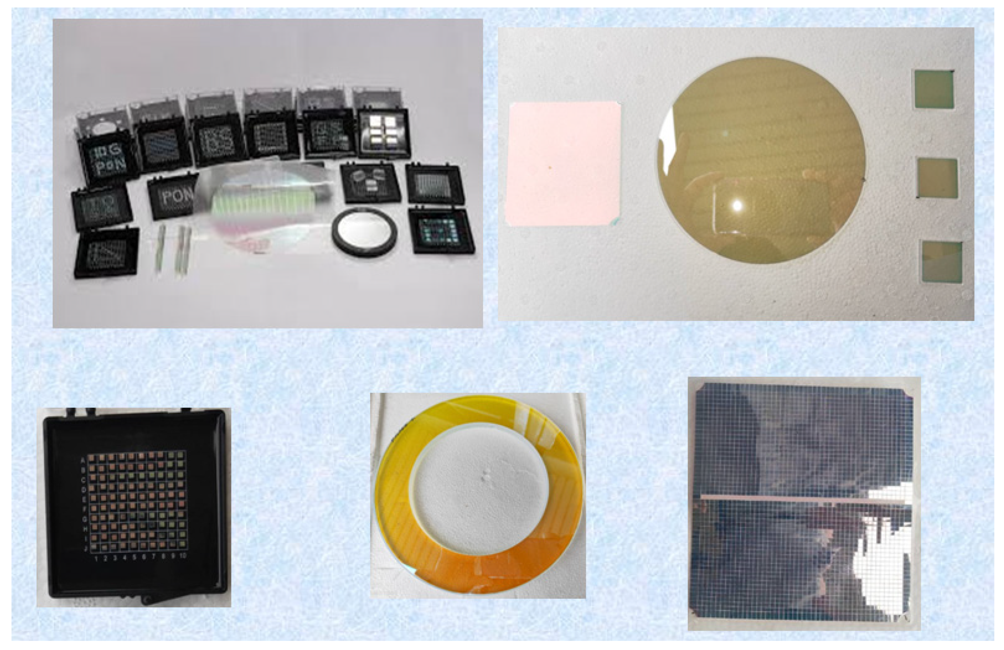
Figure 1. Related products in the optical filter industry.
Axioms 13 00054 g001
Figure 2. Research architecture of this study.
Axioms 13 00054 g002
Figure 3. The flowchart of processing optical filters.
Axioms 13 00054 g003
Figure 4. The flowchart of processing data mining functions.
Axioms 13 00054 g004
Figure 5. A diagram of PID temperature controller architecture.
Axioms 13 00054 g005
Figure 6. Research flow chart of this study.
Axioms 13 00054 g006
Figure 7. Flow chart of further data analysis for the hybrid proposed model.
Axioms 13 00054 g007
Figure 8. The processing environment diagram for Type I of the fuzzy control PID.
Axioms 13 00054 g008
Figure 9. The architecture diagram of the fuzzy control PID.
Axioms 13 00054 g009
Figure 10. The diagram of input and output values for the fuzzy control.
Axioms 13 00054 g010
Figure 11. Input e of membership function diagram for the fuzzy control.
Axioms 13 00054 g011
Figure 12. Fuzzy decision rule base for the fuzzy control PID.
Axioms 13 00054 g012
Figure 13. Processing flow of fine-tuning ΔKp, ΔKi, and ΔKd by fuzzy control after tuning PID adjustment.
Axioms 13 00054 g013
Figure 14. Results of the fine-tuning ΔKp, ΔKi, and ΔKd by the fuzzy control PID.
Axioms 13 00054 g014
Figure 15. Membership function of input e using the fuzzy control.
Axioms 13 00054 g015
Figure 16. Decision rules of fuzzy-rules based of the fuzzy control PID + ΔKp, ΔKi, and ΔKd.
Axioms 13 00054 g016
Figure 17. Architecture of a NN model.
Axioms 13 00054 g017
Figure 18. Distribution status of the yield rate for the case study.
Axioms 13 00054 g018
Figure 19. Verification results for line chart of NN model.
Axioms 13 00054 g019
Table 1. Original partial data collected from an optoelectronic company.
P.M.J.N.P.C.E.C.S.S.Y.R.C.F.Y.D.S.T.C.T.C.W.T.I.W.P.R.W.P.Ta2O5SiO2Result
JanuaryG2101001100GK011951.16131951842040.6−1−1.5B
JanuaryG2101002MBSB00215020.1 2195185202.40.600.5B
JanuaryG2101003100GC0039538.5 2178179212.80.630.5N
JanuaryG2101004800GA00115036.6 217518020.53.30.80−0.5N
JanuaryG2101005MBBD0049534.28 6178193212.50.820N
JanuaryG2101006100GF0069535.47 6201185202.80.621N
JanuaryG2101007100GJ0109501818820823.53.60.20−0.5B
JanuaryG2101008100GI0099520.42102177183193.80.9−21.5B
JanuaryG2101009CWDME00515082.76 6176175212.80.800G
JanuaryG2101010800GG00715038.20 621518020.52.80.9−20N
JanuaryG2101011MWBH0081507.082317618519.53.60.103.5B
JanuaryG2101012100GK0119515.99 31841842040.6−1−4.5B
JanuaryG2101013800GA00115065.53 617618020.53.30.80−0.5G
JanuaryG2101014MBSB00215090.21 6195185202.40.61−1G
JanuaryG2101015100GC0039531.53 2180178212.80.630.5N
JanuaryG2101016100GF0069537.30 420018720.52.70.441.5N
JanuaryG2101017MBBD0049544.92 2178193212.50.801N
JanuaryG2101018100GJ0109518.81 318821123.53.60.20−1.5B
JanuaryG2101019CWDME00515053.99 6176178212.80.80−0.5N
JanuaryG2101020100GI0099539.01 217817818.53.81.000.5N
JanuaryG2101021800GG00715030.62 2212181202.80.6−20N
JanuaryG2101022800GA00115087.77 6176179203.30.800G
JanuaryG2101023MWBH00815028.63 217618819.53.60.100.5B
JanuaryG2101024100GK0119514.51 4185185204.00.60−0.5B
JanuaryG2101025100GC0039533.16 218117921.52.80.520N
JanuaryG2101026MBSB00215090.21 6196185212.40.601.5G
JanuaryG2101027100GJ0109528.08 218719024.33.60.100.5B
JanuaryG2101028MBBD00495028178193212.50.800B
JanuaryG2101029CWDME0051506.2881180170212.80.600B
JanuaryG2101030800GG00715043.34 6210175202.80.6−30N
JanuaryG2101031100GI0099532.25 217718618.53.80.8−10.5N
JanuaryG2101032100GF006955.7322199188212.80.541.5B
JanuaryG2101033800GA00115060.49 6175176203.20.800G
JanuaryG2101034MBBD00495028178193212.50.800B
Table 2. Partial data after performing classification process of decision attribute.
P.M.J.N.P.C.E.C.S.S.Y.R.C.F.Y.D.S.T.C.T.C.W.T.I.W.P.R.W.P.Ta2O5SiO2T.D.Result
JanuaryG2101003100GC0039538.5 2178179212.80.630.51N
JanuaryG2101006100GF0069535.47 6201185202.80.621−10N
JanuaryG2101015100GC0039531.53 2180178212.80.630.5−2N
JanuaryG2101016100GF0069537.30 420018720.52.70.441.5−13N
JanuaryG2101020100GI0099539.01 217817818.53.81.000.50N
JanuaryG2101025100GC0039533.16 218117921.52.80.520−2N
JanuaryG2101031100GI0099532.25 217718618.53.80.8−10.59N
JanuaryG2101037100GC0039540.91 2180178212.80.640−2N
JanuaryG2101042100GF0069532.92 3202195212.80.631−7N
JanuaryG2101054100GK0119540.97 318619219.53.80.7−20.56N
JanuaryG2101064100GK0119538.34 318818919.54.00.600.51N
JanuaryG2101068100GC0039532.47 2176182212.80.620.56N
JanuaryG2101072100GF0069544.21 318518820.50.80.640.53N
JanuaryG2101075100GK0119533.47 318818819.54.00.600.50N
JanuaryG2101083100GC0039553.61 4170175212.80.620.55N
JanuaryG2101087100GK0119537.26 418818719.54.00.6−30.5−1N
JanuaryG2101088100GF0069545.15 4199189202.80.620.5−10N
JanuaryG2101093100GC0039551.06 6172178212.80.6006N
JanuaryG2101096100GK0119538.34 318418919.53.20.6005N
JanuaryG2101099100GF0069533.19 419219520.52.80.6313N
JanuaryG2101106100GK0119540.85 218618719.53.80.6−20.51N
JanuaryG2101107100GF0069533.32 4192186212.60.450.5−6N
JanuaryG2101109100GJ0109541.15 318619523.53.80.201.59N
JanuaryG2101113100GC0039535.47 2169175212.80.63−0.56N
JanuaryG2101117100GF0069555.38 4198187212.70.420.5−11N
JanuaryG2101128100GF0069539.64 4192182202.80.620.5−10N
JanuaryG2101133100GC0039546.50 2170176212.80.42−0.56N
JanuaryG2101139100GF0069539.64 2189182202.80.640.5−7N
JanuaryG2101143100GC0039533.23 2170176212.80.42−0.56N
JanuaryG2101148100GF0069551.91 4185182202.80.640.5−3N
JanuaryG2101150100GK0119549.58 6185.5186.519.53.90.6−20.51N
JanuaryG2101160100GK0119533.21 218619419.53.90.600.58N
JanuaryG2101168100GD0049555.27 617818921.52.70.8−3011N
JanuaryG2101171100GK0119547.30 618619319.53.90.600.57N
Table 3. Summary of box-and-whisker method after analytical experiments.
Item No.FeatureGoodNormalBadGood A.Normal A.Bad A.S.D.
1Substrate T.180–188 °C178–189.5 °C175–190 °C183.8 °C185.3 °C184.1 °CNo
2Cavity T.181–191 °C181–192 °C180–191 °C185.5 °C187.1 °C186.4 °CNo
3Cooling water T.19–21 °C19.5–21.5 °C19.5–21.5 °C20.33 °C20.86 °C21.16 °CNo
4Cooling water inlet P.3.3–3.8 kgs2.8–3.8 kgs2.8–3.6 kgs3.45 kgs3.32 kgs3.22 kgsNo
5Ta2o5 spot position 0~−10~−10~−1−0.54−0.14−0.16No
6Sio2 spot position0.5~−0.50.5~−0.50.5~−0.5−0.180.060.15No
7T. D. between the cavity and the substrate2~3 °C3~9 °C4~13.5 °C2.3 °C6.1 °C9.25 °CYes
Note: A. refers to average, S. refers to significant, T. refers to temperature, P. refers to pressure, and D. refers to difference.
Table 4. Summary of feature correlation from performing the association rule method.
Item No.FeatureGoodNormalBadGood A.Normal A.Bad A.S.D.
1Substrate T.175–186 °C176–188 °C175–188 °C182.1 °C183.5 °C183.4 °CNo
2Cavity T.179–190 °C180–190 °C179–190 °C185.3 °C185.2 °C184.6 °CNo
3Cooling water T.20–21 °C19.5–21.5 °C19.5–21.5 °C20.6 °C20.9 °C20.9 °CNo
4Cooling water inlet P.2.4–3.1 kgs2.8–3.6 kgs2.8–3.6 kgs2.84 kgs3.15 kgs3.16 kgsNo
5Ta2o5 spot position 0~−10~−10~−1−0.32−0.27−0.30No
6Sio2 spot position0.5~−0.50.5~−0.50.5~−0.50.050.1480.159No
7T. D. between the cavity and the substrate2~3 °C3~9 °C4~13.5 °C2.3 °C6.1 °C9.25 °CYes
Note: A. refers to average, S. refers to significant, T. refers to temperature, P. refers to pressure, and D. refers to difference.
Table 5. Summary of analysis results from the decision tree technique.
Item No.FeatureGoodNormalBadS.D.
1Substrate T.167–195.5 °C167–195.5 °C167–195.5 °CNo
2Cavity T.184.5–198 °C184.5–198 °C184.5–198 °CNo
3Cooling water T.18–22 °C18–22 °C18–22 °CNo
4Cooling water inlet P.2.1–3.4 kgs2.1–3.4 kgs2.1–3.4 kgsNo
5Ta2O5 spot position 0~+20~+20~+2No
6SiO2 spot position0~−4.50~−4.50~−4.5No
7T. D. between the cavity and the substrate≤ 2 °C2~8.59 °C8.5~17 °CYes
Yield rate %3.7%40.10%56.20%-
Note: S. refers to significant, T. refers to temperature, P. refers to pressure, and D. refers to difference.
Table 6. Parameter list of the mathematical model from the case factory.
ObjectMassSpecific HeatSurface AreaEmissivitySubstrate T.Cavity T.Cavity Wall T.Constant of P.T. SettingNormal T.
MCAεT1T2TwσTsT
g°Ccm2°C°C°C W / m 2 K 4 °C°C
Substrate25070017,66211.751751751755.67 × 10−817525
Cavity20,00050035,0000.95173–177173–177173–1775.67 × 10−817525
Cavity wall10,00050022,0000.45173–177173–177173–1775.67 × 10−817525
Note: T. refers to temperature and P. refers to proportionality.
Table 7. Verification results for the NNs model.
Temperature difference (°C)0123456
Yield rate (%)98.5798.5792.8585.7174.2871.4059.71
Temperature difference (°C)78910111213
Yield rate (%)58.5757.1454.2847.1442.8531.4222.80
Temperature difference (°C)14151617181920
Yield rate (%)15.718.575.715.714.281.420
Disclaimer/Publisher’s Note: The statements, opinions and data contained in all publications are solely those of the individual author(s) and contributor(s) and not of MDPI and/or the editor(s). MDPI and/or the editor(s) disclaim responsibility for any injury to people or property resulting from any ideas, methods, instructions or products referred to in the content.