Multi-Player Non-Cooperative Game Strategy of a Nonlinear Stochastic System with Time-Varying Parameters

Abstract

This paper discusses the multi-player non-cooperative game of nonlinear stochastic time-varying systems described by Itô-type differential equations in a finite time interval. Multi-player non-cooperative game problems are represented by multi-objective Pareto (MOP) control problems to describe the fact that each player has their own goals. By applying Hamilton–Jacobi inequalities (HJIs), the criterion of upper bounds of the MOP boundary is obtained for nonlinear stochastic systems, and the corresponding strategies are designed for such games, so the MOP problem is transformed into a HJI-constrained MOP problem. In order to overcome the difficulty of solving HJIs, a global linearization method is proposed to approximate the nonlinear systems. By the proposed global linearization method, multi-player non-cooperative game problems are transformed into Riccati equation-constrained MOP problems, and the approximate solutions of HJI-constrained MOP problems are obtained. Finally, a practical example is given to illustrate the effectiveness of the proposed method.

1. Introduction

Non-cooperative games are widely applied in various fields of natural and social sciences, such as economics, finance, and engineering technology [1,2,3]. Compared to cooperative games, the behavior and decision making of participants in non-cooperative games are independent of each other. Under proper conditions, there exists a Nash equilibrium point in the non-cooperative games [4]. To resolve the problem of multiple Nash equilibria for non-cooperative games, the concept of Pareto undominated Nash equilibrium is raised and is studied by many researchers. For example, by combining the subset of non-cooperative players with that of aggregate ones, Goldman and Shier proposed weaker conditions to solve the equilibrium-point solutions of the game and given the approximate versions to obtain the equilibrium points [5]. Using a modified fixed point theorem, Zhao, Hong and Li achieved an existence theorem of extended Nash equilibria of the nonmonetized noncooperative game [6]. Ye and Hu employed an extremum-seeking method to non-cooperative games and offered a non-model-based seeking scheme to achieve the time-varying Nash equilibrium [7]. Using the Hamilton–Jacobi–Bellman equations, Aduba and Won proposed the necessary and sufficient conditions for the Nash equilibrium solution of nonzero-sum dynamic statistical Nash games with N-player m-th cost cumulant optimization [8]. Bressan and Nguyen studied a kind of non-cooperative game in the case of infinite time horizon with exponentially discounted quadratic costs [9]. Dianetti and Ferrari established the existence of Nash equilibria for a class of N-player stochastic games with a monotone-follower type, in which the Markovian setting is not necessary and the approximation of the equilibrium values is also provided [10]. Furthermore, theories of non-cooperative or cooperative games such as vector-valued games [11], a Pareto undominated mixed-strategy [2], Nash–Stackelberg–Nash games [12] and multio-bjective games [13] have also been developed, and many excellent results have been obtained.

In practice, many economic, financial, biological or engineering systems can be described by ordinary differential equations [14,15,16,17,18] and stochastic differential equations [19,20,21,22,23,24,25] in continuous time and by difference equations [26,27,28] in a discrete-time case. For example, in order to demonstrate the interplay among interest rate, investment demand and price, the following ordinary different equation are proposed:

$$\left\{\begin{array}{c}\dot{\xi }\left(t\right)=\zeta \left(t\right)+(\eta \left(t\right)-a)\xi \left(t\right)\hfill \\ \dot{\eta }\left(t\right)=1-b\eta \left(t\right)-{\xi }^2\left(t\right)\hfill \\ \dot{\zeta }\left(t\right)=-\xi \left(t\right)-c\zeta \left(t\right)\hfill \end{array}\right.,$$

(1)

where $\xi \left(t\right)$ is the interest rate of the financial market, $\eta \left(t\right)$ is the investment demand of market participants, and $\zeta \left(t\right)$ is the reasonable market price. By solving the following equation,

$$\left\{\begin{array}{c}\zeta +(\eta -a)\xi =0\hfill \\ 1-b\eta -{\xi }^2=0\hfill \\ -\xi -c\zeta =0\hfill \end{array}\right.,$$

(2)

it’s easy to find that one of the equilibria of System (1) is

$$[{\xi }_{eq},{\eta }_{eq},{\zeta }_{eq}]=[\pm \sqrt{1-\frac{b}{c}-ab},\frac{1}{c}+a,\mp \frac{1}{c}\sqrt{1-\frac{b}{c}-ab}].$$

In the real word, the equilibrium points of an economic systems or financial systems are changing at different times, which implies that parameters $a,b$ and c in System (1) change over time. Moreover, taking into account inherent stochastic fluctuations and external disturbances, the following stochastic dynamic system is constructed in reference [23]:

$$\left\{\begin{array}{c}d\xi \left(t\right)=[\zeta \left(t\right)+(\eta \left(t\right)-a)\xi \left(t\right)+u_1\left(t\right)+b_{12}{u}_2\left(t\right)+b_{31}{u}_3\left(t\right)\hfill \\ +v_1\left(t\right)]dt+\xi \left(t\right)]dW\left(t\right)\hfill \\ d\eta \left(t\right)=[1-b\eta \left(t\right)-{\xi }^2\left(t\right)+b_{21}{u}_1\left(t\right)+u_2\left(t\right)+b_{23}{u}_3\left(t\right)\hfill \\ +v_2\left(t\right)]dt+\eta \left(t\right)dW\left(t\right)\hfill \\ d\zeta \left(t\right)=[-\xi \left(t\right)-c\zeta \left(t\right)+b_{31}{u}_1\left(t\right)+b_{32}{u}_2\left(t\right)+u_3\left(t\right)\hfill \\ +v_3\left(t\right)]dt+\zeta \left(t\right)dW\left(t\right)\hfill \end{array}\right.,$$

(3)

where $u_i\left(t\right)$ denotes strategies ($i=1,2,3$), $v\left(t\right)={[v_1\left(t\right),v_2\left(t\right),v_3\left(t\right)]}^T$ is the exogenous disturbance, $W\left(t\right)$ is the one-dimensional standard Brownian motion. In this model, the influence of government control strategy, investment strategy of bank consortium and investment strategy of the public on the stability of the financial system are considered to obtain the non-cooperative investment strategies for financial markets. According to the global linearization technique [20,29], the multi-objective problem (MOP) with the Hamilton–Jacobi inequality (HJI) constraint is transformed into MOP with an equivalent Linear matrix inequality (LMI) constraint to solve the non-cooperative game problems discussed in [23] in which the financial systems are described by time-invariant stochastic differential equations. These results are based on the help of Riccati equations or Riccati inequalities for linear systems [30,31].

Against the above -mentioned background, the time-varying systems are used to describe such systems as follows:

$$\left\{\begin{array}{c}d\xi \left(t\right)=[\zeta \left(t\right)+(\eta \left(t\right)-a\left(t\right))\xi \left(t\right)+u_1\left(t\right)+b_{12}{u}_2\left(t\right)+b_{13}{u}_3\left(t\right)\hfill \\ +v_1\left(t\right)]dt+\xi \left(t\right)]dW\left(t\right)\hfill \\ d\eta \left(t\right)=[1-b\left(t\right)\eta \left(t\right)-{\xi }^2\left(t\right)+b_{21}{u}_1\left(t\right)+u_2\left(t\right)+b_3{u}_3\left(t\right)\hfill \\ +v_2\left(t\right)]dt+\eta \left(t\right)dW\left(t\right)\hfill \\ d\zeta \left(t\right)=[-\xi \left(t\right)-c\left(t\right)\zeta \left(t\right)+b_{31}{u}_1\left(t\right)+b_{32}{u}_2\left(t\right)+u_3\left(t\right)\hfill \\ +v_3\left(t\right)]dt+\zeta \left(t\right)dW\left(t\right)\hfill \end{array}\right..$$

(4)

So conditions such as Hamilton–Jacobi equations or inequalities and Riccati equations for corresponding non-cooperative games of time-varying systems are also different from those of the time-invariant ones, which needs further study. This paper follows the line of [23] to discuss the non-cooperative games for nonlinear stochastic time-varying systems, and, in comparison to [23], this paper has the following novelty and innovation: (1) The systems discussed in this paper have more general forms which consider the time-varying case. (2) Because the Riccati equations, the Hamilton-Jacobi equations and matrices used in this paper are in the time-varying form, the global linear methods are more complex than the methods given by [23]. This paper is organized as follows: In Section 2, some theories of stochastic differential equations are reviewed, and the non-cooperative games for stochastic time-varying systems are described. In Section 3, the multi-party non-cooperative investment strategies for nonlinear time-varying stochastic financial systems are designed with the help of solving Hamilton–Jacobi inequalities for nonlinear systems and Riccati equations for linear systems. In Section 4, a global linearization method for a nonlinear stochastic financial system with time-varying parameters is proposed, which transforms an HJI-constrained MOP to an LMI-constrained MOP. In Section 5, a practical financial example is illustrated to verify the effectiveness of the proposed method.

Notations: $\mathbb{T}$: finite time interval $[0,T]$, $0<T<\infty$; $n_v$: dimension of vector v; $A^T$ or $x^T$: transport of matrix A or vector x; $|x|$: Euclidean norm of vector x; $\mathbb{E}\left[X\right]$: expectation of random variable X; $A>0(A\ge 0)$: symmetric real matrix A is a (semi-) positive definite matrix.

2. Preliminary

Suppose $(\mathsf{\Omega },\mathcal{F},\mathbb{P})$ is a complete probability space. An economic or financial system with m-person decision makers can be described by the following time-varying stochastic differential equations:

$$\left\{\begin{array}{c}d\xi \left(t\right)=[f(t,\xi \left(t\right))+{\displaystyle \sum _{i=1}^m}{g}_i(t,\xi \left(t\right))u_i\left(t\right)+h(t,\xi \left(t\right))v\left(t\right)]dt\hfill \\ +[l(t,\xi \left(t\right))+h_1(t,\xi \left(t\right))v\left(t\right)]dW\left(t\right)\hfill \\ \xi \left(0\right)={\xi }_0\in {\mathbb{R}}^n,t\in \mathbb{T}=[0,T],0<T<\infty \hfill \end{array}\right.,$$

(5)

where $f:(\mathbb{T},{\mathbb{R}}^n)\to {\mathbb{R}}^n$, $g_i:(\mathbb{T},{\mathbb{R}}^n)\to {\mathbb{R}}^{m\times n_{u_i}}$, $h:(\mathbb{T},{\mathbb{R}}^n)\to {\mathbb{R}}^{n\times n_v}$, $l:(\mathbb{T},{\mathbb{R}}^n)\to {\mathbb{R}}^n$, $h_1:(\mathbb{T},{\mathbb{R}}^n)\to {\mathbb{R}}^{n\times n_v}$$x={[{\xi }_1\left(t\right),\cdots ,{\xi }_i\left(t\right)\cdots ,{\xi }_n\left(t\right)]}^T$ denotes the state vector of economic or financial system, $u_i\left(t\right)$ denotes the ith agent’s strategies or policies, $v\left(t\right)$ is the external disturbance, $W\left(t\right)$ is a one-dimensional normal Brownian motion.

The goal of the ith agent is to maximize their profit returns or to minimize their return risk. The ith agent’s game strategy $u_i$ is decided under the background of the strategies of other $m-1$ agents with $u_1\left(t\right),\cdots ,u_{i-1}\left(t\right),u_{i+1}\left(t\right)\cdots ,u_m\left(t\right)$ which are unknown to the ith agent. Since external disturbance $v\left(t\right)$ also plays an important role and is not available to every participant including the ith agent, its impact on the financial system must be considered from the worst case. Each agent tends to minimize the worst-case effects of external distractions.

In a non-cooperative financial system, for the ith agent, it is difficult to obtain all other strategies and external distractions. Thus, each game strategy $u_i\left(t\right)$ of an ith player tries to minimize the worst case effects of both a combination of competitive strategies and external distractions to achieve the desired target, ${\xi }_{di}$. So the goals of the ith agent can be modeled by

$$\begin{array}{ccc}\hfill & & r_i^{*}=\underset{u_i\left(t\right)}{min}\underset{u_{-i}\left(t\right)}{max}\frac{\mathbb{E}{\int }_0^T[{(\xi \left(t\right)-{\xi }_{di})}^T{Q}_i(\xi \left(t\right)-{\xi }_{di})+u_i^T\left(t\right)R_i{u}_i\left(t\right)]dt}{\mathbb{E}{(\xi \left(0\right)-{\xi }_{di})}^T(\xi \left(0\right)-{\xi }_{di})+\mathbb{E}{\int }_0^T|u_{-i}{|}^2\left(t\right)dt+\mathbb{E}{\int }_0^T{|v\left(t\right)|}^{2}dt}\hfill \\ & & i=1,2,\cdots ,m,\hfill \end{array}$$

(6)

where $u_{-i}\left(t\right)={[u_1^T\left(t\right),\cdots ,u_{i-1}^T\left(t\right),u_{i+1}^T\left(t\right),\cdots ,u_m^T\left(t\right)]}^T$, $Q_i>0$ and $R_i>0$ are weight matrices.

Denote ${\widehat{\xi }}_i\left(t\right)={\xi }_i\left(t\right)-{\xi }_{di}$ and $\widehat{\xi }\left(t\right)=\xi \left(t\right)-{\xi }_{di}$, then the goals of (6) can be simplified as

$$\begin{array}{ccc}\hfill & & r_i^{*}=\underset{u_i\left(t\right)}{min}\underset{u_{-i}\left(t\right)}{max}\frac{\mathbb{E}{\int }_0^T[\widehat{\xi }{\left(t\right)}^T{Q}_i\widehat{\xi }\left(t\right)+u_i^T\left(t\right)R_i{u}_i\left(t\right)]dt}{\mathbb{E}[|\widehat{\xi }{\left(0\right)|}^2]+\mathbb{E}{\int }_0^T|u_{-i}{|}^2\left(t\right)dt+\mathbb{E}{\int }_0^T{|v\left(t\right)|}^{2}dt}\hfill \\ & & i=1,2,\cdots ,m.\hfill \end{array}$$

(7)

under constraint

$$\left\{\begin{array}{c}d\widehat{\xi }\left(t\right)=[\widehat{f}(t,\widehat{\xi }\left(t\right))+{\displaystyle \sum _{i=1}^m}{\widehat{g}}_i(t,\widehat{\xi }\left(t\right))u_i\left(t\right)+\widehat{h}(t,\widehat{\xi }\left(t\right))v\left(t\right)]dt\hfill \\ +[\widehat{l}(t,\widehat{\xi }\left(t\right))+{\widehat{h}}_1(t,\widehat{\xi }\left(t\right))v\left(t\right)]dW\left(t\right)\hfill \\ \widehat{\xi }\left(0\right)={\xi }_0-{\xi }_{di}\in {\mathbb{R}}^n,t\in \mathbb{T}=[0,T],0<T<\infty \hfill \end{array}\right.,$$

(8)

where $\widehat{\phi }(t,\widehat{\xi })=\phi (t,\widehat{\xi }+{\xi }_{di})$, $\phi =f,g,h,l,h_1$.

So the m-agent noncooperative game strategy $(u_1^{*},u_2^{*},\cdots ,u_m^{*})$ of multi-objective Pareto problems (5)–(6) or (7)–(8) can be seen as a Nash equilibrium if and only if [4]

$$\left\{\begin{array}{cc}\hfill (r_1^{*},r_2^{*},\cdots ,r_m^{*})& \le (r_1,r_2^{*},\cdots ,r_m^{*})\hfill \\ \hfill & \cdots \hfill \\ \hfill (r_1^{*},\cdots ,r_i^{*},\cdots ,r_m^{*})& \le (r_1^{*},\cdots ,r_{i-1}^{*},r_i,r_{i+1}^{*},\cdots ,r_m^{*})\hfill \\ \hfill & \cdots \hfill \\ \hfill (r_1^{*},r_2^{*},\cdots ,{\rho }_{m-1}^{*},r_m^{*})& \le (r_1^{*},r_2^{*},\cdots ,{\rho }_{m-1}^{*},r_m)\hfill \end{array}\right.,$$

(9)

where $(r_1^{*},r_2^{*},\cdots ,r_m^{*})$ is the Pareto boundary of multi-objective problems (MOPs) (5) and (6), i.e.,

$$\begin{array}{c}\hfill \begin{array}{c}\hfill (r_1^{*},\cdots ,r_i^{*},\cdots ,r_m^{*})=\underset{u}{min}(r_1,\cdots ,r_i,\cdots ,r_m)\end{array}.\end{array}$$

(10)

Because stochastic Systems (5) and (8) are presented by Itô-type differential equations, the existence and uniqueness of solutions of such systems can be obtained by the following Lemma 1.

Lemma 1.

Suppose the Itô-type stochastic differential equations (SDEs) driven by a one-dimensional Brownian motion are given by

$$\left\{\begin{array}{c}d\xi \left(t\right)=b(t,\xi (t\left)\right)dt+\sigma (t,\xi (t\left)\right)dW\left(t\right)\hfill \\ \xi \left(0\right)={\xi }_0\in {\mathbb{R}}^n,t\in [0,T]\hfill \end{array}\right..$$

(11)

Coefficients $b(t,\xi )$ and $\sigma (t,\xi )$ satisfy Lipschitzian conditions

$$|b(t,{\xi }_1)-b(t,{\xi }_1)|+|\sigma (t,{\xi }_1)-\sigma (t,{\xi }_2)|\le C_1|{\xi }_1-{\xi }_2|,\forall {\xi }_1,{\xi }_2\in {\mathbb{R}}^n,$$

and

$$|b(t,\xi )|+|\sigma (t,\xi )|\le C_2|\xi |,\forall \xi \in {\mathbb{R}}^n,$$

  for some constant  $C_1$  and  $C_2$. Then, SDE (11) exists as a unique solution.

The following Itô formula of SDEs will be used in the proofs of our main results.

Lemma 2.

Suppose $V(t,\xi )\in C^{1,2}([0,T],{\mathbb{R}}^n)$ and $\left\{\xi \right(t),t\in [0,T\left]\right\}$ is the solution of SDE (11), then the following Itô formula is obtained:

$$\begin{array}{c}\hfill dV(t,\xi \left(t\right))=[V_t(t,\xi \left(t\right))+V_{\xi }^T(t,\xi \left(t\right))f(t,\xi \left(t\right))+\frac{1}{2}{\sigma }^T(t,\xi \left(t\right))V_{xx}\sigma (t,\xi \left(t\right))]dt\\ \hfill +V_{\xi }^T(t,\xi \left(t\right))\sigma (t,x)dW\left(t\right),\end{array}$$

(12)

where $V_t$ and $V_{\xi }$ are first-order partial derivatives w.r.t. t and x, respectively, with

$$V_{\xi }={\left[\frac{\partial V}{\partial {\xi }_1},\frac{\partial V}{\partial {\xi }_2},\cdots ,\frac{\partial V}{\partial {\xi }_n}\right]}^T,$$

and $V_{xx}$ is the second-order partial derivatives w.r.t. x defined as

$$V_{xx}=\left[\begin{array}{cccc}\frac{{\partial }^{2}V}{\partial {\xi }_1^2}& \frac{{\partial }^{2}V}{\partial {\xi }_1\partial {\xi }_2}& \cdots & \frac{{\partial }^{2}V}{\partial {\xi }_1\partial {\xi }_n}\\ \frac{{\partial }^{2}V}{\partial {\xi }_2{\xi }_1}& \frac{{\partial }^{2}V}{\partial {\xi }_2^2}& \cdots & \frac{{\partial }^{2}V}{\partial {\xi }_2\partial {\xi }_n}\\ ⋮& ⋮& & ⋮\\ \frac{{\partial }^{2}V}{\partial {\xi }_n{\xi }_1}& \frac{{\partial }^{2}V}{\partial {\xi }_n{\xi }_2}& \cdots & \frac{{\partial }^{2}V}{\partial {\xi }_n^2}\end{array}\right].$$

3. Multi-Party Non-Cooperative Investment Strategies for Time-Varying Stochastic Financial Systems

To simplify the calculation, we let the desired target ${\xi }_{di}=0,i=1,2,\cdots ,m$. So the solutions of (5) of (8) are equivalent, i.e., ${\widehat{\xi }}_i\left(t\right)=\xi \left(t\right)$. The MOP problems of (5)–(6) and (7)–(8) convert to the following multi-objective problem:

$$\begin{array}{ccc}\hfill & & r_i^{*}=\underset{u_i\left(t\right)}{min}\underset{u_{-i}\left(t\right)}{max}\frac{\mathbb{E}{\int }_0^T[\xi {\left(t\right)}^T{Q}_i\xi \left(t\right)+u_i^T\left(t\right)R_i{u}_i\left(t\right)]dt}{\mathbb{E}\xi {\left(0\right)}^T\xi \left(0\right)+\mathbb{E}{\int }_0^T|u_{-i}{|}^2\left(t\right)dt+\mathbb{E}{\int }_0^T{|v\left(t\right)|}^{2}dt},\hfill \\ & & i=1,2,\cdots ,m.\hfill \end{array}$$

(13)

subject to

$$\left\{\begin{array}{c}d\xi \left(t\right)=[f(t,\xi \left(t\right))+{\displaystyle \sum _{i=1}^m}{g}_i(t,\xi \left(t\right))u_i\left(t\right)+h(t,\xi \left(t\right))v\left(t\right)]dt\hfill \\ +[l(t,\xi \left(t\right))+h_1(t,\xi \left(t\right))v\left(t\right)]dW\left(t\right)\hfill \\ \xi \left(0\right)={\xi }_0\in {\mathbb{R}}^n,f(t,0)\equiv 0,l(t,0)\equiv 0,t\in [0,T],0<T<\infty \hfill \end{array}\right..$$

(14)

In System (14), $x=0$ is the equilibrium point. Namely, only the stabilization issue is considered in traditional non-cooperative game strategies. In order to obtain the MOP solution $(r_1^{*},r_2^{*},\cdots ,r_m^{*})$ and strategies $(u_1^{*},u_2^{*},\cdots ,u_m^{*})$, for every i, we first offer $r_i>0$ as the upper bound of $r_i^{*}$, i.e., $r_i^{*}\le r_i$ with $u_i=u_i^{*}$. So the following inequality can be obtained when $u_i=u_i^{*}$:

$$\begin{array}{ccc}& & \underset{u_{-i}\left(t\right)}{max}\frac{\mathbb{E}{\int }_0^T[\xi {\left(t\right)}^T{Q}_i\xi \left(t\right)+u_i^T\left(t\right)R_i{u}_i\left(t\right)]dt}{\mathbb{E}\xi {\left(0\right)}^T\xi \left(0\right)+\mathbb{E}{\int }_0^T|u_{-i}{|}^2\left(t\right)dt+\mathbb{E}{\int }_0^T{|v\left(t\right)|}^{2}dt}\le r_i.\hfill \end{array}$$

So, for every $u_{-i}\left(t\right)$ and $v\left(t\right)$, there exists

$$\begin{array}{ccc}& & \frac{\mathbb{E}{\int }_0^T[\xi {\left(t\right)}^T{Q}_i\xi \left(t\right)+u_i^T\left(t\right)R_i{u}_i\left(t\right)]dt}{\mathbb{E}\xi {\left(0\right)}^T\xi \left(0\right)+\mathbb{E}{\int }_0^T|u_{-i}{|}^2\left(t\right)dt+\mathbb{E}{\int }_0^T{|v\left(t\right)|}^{2}dt}\le r_i\hfill \end{array}$$

which equals to

$$\begin{array}{c}\hfill \mathbb{E}{\int }_0^T[\xi {\left(t\right)}^T{Q}_i\xi \left(t\right)+u_i^T\left(t\right)R_i{u}_i\left(t\right)]dt\le r_i\mathbb{E}\left[{|\xi \left(0\right)|}^2+{\int }_0^T|u_{-i}{|}^2\left(t\right)dt+{\int }_0^T{|v\left(t\right)|}^{2}dt\right].\end{array}$$

Let

$$\begin{array}{c}\hfill J_i(u,v)=\mathbb{E}\left\{{\int }_0^T{[\xi \left(t\right)}^T{Q}_i\xi \left(t\right)+u_i^T\left(t\right)R_i{u}_i\left(t\right)-r_i|u_{-i}{\left(t\right)|}^2-r_i{\int }_0^T{|v\left(t\right)|}^2]dt-r_i{|\xi \left(0\right)|}^2\right\}.\end{array}$$

(15)

Then, $r_i$ is the upper bound of $r_i^{*}$ with $u_i=u_i^{*}$ if and only if, for every $u_{-i}$ and v, there exists

$$J_i(u_i^{*},u_{-i},v)\le 0.$$

Theorem 1.

For a given $r_i>0$, if there exists $V(t,x)\in C^{1,2}([0,T],{\mathbb{R}}^n)$, it satisfies the following Hamilton–Jacobi inequality (HJI):

$$\left\{\begin{array}{c}\mathcal{H}\left(V\right)(t,x):=V_t+V_x^{T}f(t,x)+\frac{1}{2}{l}^T(t,x)V_{xx}l(t,x)+x^T{Q}_{i}x\hfill \\ -\frac{1}{4}{V}_x^T{g}_i(t,x)R_i^{-1}{g}_i^T(t,x)V_{\xi }+\frac{1}{4r_i}{V}_x^T{g}_{-i}(t,x)g_{-i}^T(t,x)V_{\xi }\hfill \\ +\frac{1}{4}(V_x^{T}h(t,x)+l^T(t,x)V_{xx}{h}_1(t,x))\hfill \\ \times {\left(r_{i}I-\frac{1}{2}{h}_1^T(t,x)V_{xx}{h}_1(t,x)\right)}^{-1}\hfill \\ \times (h^T(t,x)V_x^T+h_1^T(t,x)V_{xx}l(t,x))\le 0,\hfill \\ r_{i}I-\frac{1}{2}{h}_1^T(t,x)V_{xx}{h}_1(t,x)>0,\forall (t,x)\in [0,T]\times {\mathbb{R}}^n,\hfill \\ V(T,x)\equiv 0,V(0,x)\le r_i{|x|}^2\forall x\in {\mathbb{R}}^n,\hfill \end{array}\right.$$

(16)

then $r_i$ is a upper bound of ${\rho }^{*}$ of MOP problems (13) and (14) with

$$u_i^{*}\left(t\right)=-\frac{1}{2}{R}_i^{-1}{g}_i^T(t,\xi \left(t\right))V_{\xi }(t,\xi \left(t\right)).$$

(17)

Proof. 

Applying the Itô formula to $V(t,\xi (t\left)\right)$, we obtain

$$\begin{array}{c}\hfill dV(t,\xi \left(t\right))=[V_t(t,\xi \left(t\right))+V_x^T(t,\xi \left(t\right))(f(t,\xi \left(t\right))+\sum _{i=1}^m{g}_i(t,\xi \left(t\right))u_i\left(t\right)+h(t,\xi \left(t\right))v\left(t\right))\\ \hfill +\frac{1}{2}(v^T\left(t\right)h_1^T(t,\xi \left(t\right))+l^T(t,\xi \left(t\right)))V_{xx}(t,\xi \left(t\right))(l(t,\xi \left(t\right))+h_1(t,\xi \left(t\right))v\left(t\right))]dt\\ \hfill +V_x^T(t,\xi \left(t\right))(l(t,\xi \left(t\right))+h_1(t,\xi \left(t\right))v\left(t\right))dW\left(t\right).\end{array}$$

Integrating on $[0,T]$, then taking expectation on both sides, we obtain

$$\begin{array}{ccc}& & \mathbb{E}\left[V(T,\xi \left(t\right))\right]-\mathbb{E}\left[V(0,\xi \left(0\right))\right]=\mathbb{E}{\int }_0^T[V_t(t,\xi \left(t\right))+V_x^T(t,\xi \left(t\right))(f(t,\xi \left(t\right))\hfill \\ & & +\sum _{i=1}^m{g}_i(t,\xi \left(t\right))u_i\left(t\right)+h(t,\xi \left(t\right))v\left(t\right))+\frac{1}{2}(v^T\left(t\right)h_1^T(t,\xi \left(t\right))+l^T(t,\xi \left(t\right)))\hfill \\ & & \times V_{xx}(t,\xi \left(t\right))(l(t,\xi \left(t\right))+h_1(t,\xi \left(t\right))v\left(t\right))]dt.\hfill \end{array}$$

Since $V(T,x)\equiv 0$, we have

$$\begin{array}{ccc}& & 0=\mathbb{E}{\int }_0^T[V_t(t,\xi \left(t\right))+V_x^T(t,\xi \left(t\right))(f(t,\xi \left(t\right))+\sum _{i=1}^m{g}_i(t,\xi \left(t\right))u_i\left(t\right)\hfill \\ & & +h(t,\xi \left(t\right))v\left(t\right))+\frac{1}{2}(v^T\left(t\right)h_1^T(t,\xi \left(t\right))+l^T(t,\xi \left(t\right)))V_{xx}(t,\xi \left(t\right))\hfill \\ & & \times (l(t,\xi \left(t\right))+h_1(t,\xi \left(t\right))v\left(t\right))]dt-\mathbb{E}\left[V(0,\xi \left(0\right))\right].\hfill \end{array}$$

So

$$\begin{array}{ccc}& & J_i(u,v)=\mathbb{E}\left\{{\int }_0^T[V_t(t,\xi \left(t\right))+V_x^T(t,\xi \left(t\right))(f(t,\xi \left(t\right))+\frac{1}{2}{l}^T(t,\xi \left(t\right))V_{xx}(t,\xi \left(t\right))l(t,\xi \left(t\right))\right.\hfill \\ & & +x^T\left(t\right)Q_i\xi \left(t\right)+V_x^T(t,\xi \left(t\right))g_i(t,\xi \left(t\right))u_i\left(t\right)+u_i^T\left(t\right)R_i{u}_i\left(t\right)\hfill \\ & & +V_x^T(t,\xi \left(t\right))\sum _{j\ne i}^m{g}_j(t,\xi \left(t\right))u_j\left(t\right)-r_i{|u_{-i}|}^2\hfill \\ & & +V_x^T(t,\xi \left(t\right))h(t,\xi \left(t\right))v\left(t\right)+\frac{1}{2}{v}^T\left(t\right)h_1^T(t,\xi \left(t\right))V_{xx}(t,\xi \left(t\right))h_1(t,\xi \left(t\right))v\left(t\right)\hfill \\ & & \left.+l^T(t,\xi \left(t\right))V_{xx}(t,\xi \left(t\right))h_1(t,\xi \left(t\right))v\left(t\right)-r_i{|v\left(t\right)|}^2]dt-\mathbb{E}\left[V(0,\xi \left(0\right))\right]\right\}.\hfill \end{array}$$

Completing the square w.r.t. $u_i\left(t\right)$, $u_{-i}\left(t\right)$ and $v\left(t\right)$, respectively, on the integral part of the right side, we have

$$\begin{array}{ccc}& & J_i(u_i^{*},u_{-i},v)=\mathbb{E}{\int }_0^T[\mathcal{H}\left(V\right)(t,\xi \left(t\right))+{\parallel u_i+\frac{1}{2}{R}_i^{-1}{g}_i^T(t,\xi \left(t\right))V_{\xi }(t,\xi \left(t\right))\parallel }_{R_i}^2\hfill \\ & & -\parallel u_{-i}-\frac{1}{2r_i}{g}_{-i}^T(t,\xi \left(t\right))V_{\xi }{(t,\xi \left(t\right))\parallel }_{r_i}^2\hfill \\ & & -\parallel v-\frac{1}{2}{(r_{i}I-\frac{1}{2}{h}_1^T(t,\xi \left(t\right))V_{xx}(t,\xi \left(t\right))h_1^T(t,\xi \left(t\right)))}^{-1}\left(h^T(t,\xi \left(t\right))\right){\parallel }_H^2]dt,\hfill \end{array}$$

where notation ${\parallel y\parallel }_A^2:=y^{T}Ay$ with $A>0$ and $H=r_{i}I-\frac{1}{2}{h}_1^T(t,\xi \left(t\right))V_{xx}(t,\xi \left(t\right))h_1^T(t,\xi \left(t\right))$. Keeping Hamilton–Jacobi inequality (16), when $u\left(t\right)=u^{*}\left(t\right)$, for every $u_{-i}$ and v, we obtain

$$J_i(u_i^{*},u_{-i},v)\le 0.$$

So $r_i$ is an upper bound of ${\rho }^{*}$ of MOP problems (13)–(14). □

We let

$$\mathcal{V}=\left\{(V,r_i)|V(t,x)\in C^{1,2}([0,T],{\mathbb{R}}^n),V \mathrm{a}\mathrm{n}\mathrm{d} r_i>0 \mathrm{s}\mathrm{a}\mathrm{t}\mathrm{i}\mathrm{s}\mathrm{f}\mathrm{i}\mathrm{e}\mathrm{s}\mathrm{ }\mathrm{H}\mathrm{J}\mathrm{I}\left(16\right)\right\};$$

(18)

then, the Pareto boundary $r_i^{*}$ of MOP (13) and (14) can be obtained by following form:

$$r_i^{*}=\underset{(V,r_i)\in \mathcal{V}}{min}{r}_i.$$

So the MOP problems of (13) for nonlinear System (14) can be transformed to an HJI-constraint MOP,

$$\begin{array}{c}\hfill \begin{array}{c}\hfill (r_1^{*},\cdots ,r_i^{*},\cdots ,r_m^{*})=\underset{(V,r_i)\in \mathcal{V}}{min}(r_1,\cdots ,r_i,\cdots ,r_m).\end{array}\end{array}$$

(19)

Now, a linear stochastic system is considered, which is given as the following:

$$\left\{\begin{array}{c}d\xi \left(t\right)=[A\left(t\right)\xi \left(t\right)+{\displaystyle \sum _{i=1}^m}{B}_i\left(t\right)u\left(t\right)+C\left(t\right)v\left(t\right)]+[A_1\left(t\right)\xi \left(t\right)+C_1\left(t\right)v\left(t\right)]dW\left(t\right)\hfill \\ \xi \left(0\right)={\xi }_0\in {\mathbb{R}}^n\hfill \end{array}\right.,$$

(20)

with multi-objective Problem (13); then, the results of Theorem 1 described by the Hamilton equation can be obtained as the following proposition with a Riccati equation form.

Proposition 1.

For a given $r_i>0$, if there exists symmetric matrix $P_t$, it satisfies the following Riccati equation:

$$\begin{array}{c}\hfill \left\{\begin{array}{c}-{\dot{P}}_t=P_{t}A\left(t\right)+A^T\left(t\right)P_t+A_1^T\left(t\right)P_t{A}_1\left(t\right)+Q_i-P_t{B}_i\left(t\right)R_i^{-1}{B}_i^T\left(t\right)P_t\hfill \\ +\frac{1}{r_i}{P}_t{B}_{-i}\left(t\right)B_{-i}^T\left(t\right)P_t+Q_i-P_t{B}_i\left(t\right)R_i^{-1}{B}_i^T\left(t\right)P_t+\frac{1}{r_i}{P}_t{B}_{-i}\left(t\right)B_{-i}^T\left(t\right)P_t\hfill \\ +\left(P_{t}C\left(t\right)+A_1^T\left(t\right)P_t{C}_1\left(t\right)\right){\left(r_{i}I-C_1^T\left(t\right)P_t{C}_1\left(t\right)\right)}^{-1}\left(C^T\left(t\right)P_t+C_1^T\left(t\right)P_t{A}_1\left(t\right)\right)\hfill \\ r_{i}I-C_1^T\left(t\right)P_t{C}_1\left(t\right)>0,r_{i}I-P_0\ge 0\hfill \end{array}\right.;\end{array}$$

(21)

then, $r_i$ is an upper bound of $r_i^{*}$ of MOP problems (13) and (20) with

$$u_i^{*}\left(t\right)=-R_i^{-1}{B}_i^T(t,\xi \left(t\right))P_t\xi \left(t\right).$$

(22)

Proof. 

We let $V(t,x)=x^T{P}_{t}x$. We note the following facts:

$$V_t(t,x)=x^T{\dot{P}}_{t}x,V_{\xi }(t,x)=2P_{t}x,V_{xx}(t,x)=2P_t,$$

and the coefficients of nonlinear System (14) are specialized by

$$f(t,x)=A\left(t\right)x,g_i(t,x)=B_i\left(t\right),h(t,x)=C\left(t\right),l(t,x)=A_1\left(t\right)x,h_1(t,x)=C_1\left(t\right).$$

It’s easy to show that $V(t,x)=x^T{P}_{t}x$ satisfies HJIs (16). By Theorem 1, $r_i$ is an upper bound of $r_i^{*}$ and the optimal controller $u_i^{*}\left(t\right)$ given by (22). □

Remark 1.

Compared to Hamilton–Jacobi inequalities and Riccati equations applied in [23], the Hamilton–Jacobi inequalities (16) and Riccati equations (21) are all time-varying forms.

4. The Global Linearization Method for a Nonlinear Stochastic Financial System with Time-Varying Parameters

Generally, it is difficult to solve HJIs (16). In this section, a global linearization method is proposed to obtain an approximate solution of multi-objective Problem (14) with the constrain of nonlinear stochastic financial System (14). We suppose the global linearized systems of a nonlinear stochastic financial system in (14) are bounded by a polytope given as follows:

$$\left[\begin{array}{c}\frac{\partial f(t,x)}{\partial x}\\ \frac{\partial g_i(t,x)}{\partial x}\\ \frac{\partial h(t,x)}{\partial x}\\ \frac{\partial h_1(t,x)}{\partial x}\end{array}\right]\in C_0\left[\begin{array}{c}\left[\begin{array}{c}{A}_1\left(t\right)\\ B_{i1}\left(t\right)\\ C_1\left(t\right)\\ A_1^{\left(1\right)}\left(t\right)\\ C_1^{\left(1\right)}\left(t\right)\end{array}\right],\left[\begin{array}{c}{A}_2\left(t\right)\\ B_{i2}\left(t\right)\\ C_2\left(t\right)\\ A_2^{\left(1\right)}\left(t\right)\\ C_2^{\left(1\right)}\left(t\right)\end{array}\right],\cdots ,\left[\begin{array}{c}{A}_J\left(t\right)\\ B_{iJ}\left(t\right)\\ C_J\left(t\right)\\ A_j^{\left(1\right)}\left(t\right)\\ C_J^{\left(1\right)}\left(t\right)\end{array}\right]\end{array}\right],t\in [0,T].$$

(23)

The state trajectory of a nonlinear financial system of (14) can be represented by the combination of state trajectories of the following local linearized systems derived from the vertices of the polytope in (23):

$$\begin{array}{c}\left\{\begin{array}{c}d{\xi }_j\left(t\right)=[A_j\left(t\right){\xi }_j\left(t\right)+{\displaystyle \sum _{i=1}^m}{B}_{ij}\left(t\right)u_i\left(t\right)+C_j\left(t\right)v\left(t\right)]dt\hfill \\ +[A_j^{\left(1\right)}\left(t\right){\xi }_i\left(t\right)+C_j^{\left(1\right)}v\left(t\right)]dW\left(t\right),\hfill \\ {\xi }_j\left(0\right)={\xi }_0\in {\mathbb{R}}^n,j=1,2,\cdots ,J\hfill \end{array}\right.\hfill \end{array}.$$

(24)

According to the global linearization theory [29], the trajectory of the shifted financial system in (14) can be represented by a convex combination of the trajectories of these local linearized financial systems in (24) as follows:

$$\begin{array}{c}\left\{\begin{array}{c}d\xi \left(t\right)={\displaystyle \sum _{j=1}^J}{\alpha }_j(t,\xi \left(t\right))[A_j\left(t\right)\xi \left(t\right)+{\displaystyle \sum _{i=1}^m}{B}_{ij}\left(t\right)u_i\left(t\right)+C_j\left(t\right)v\left(t\right)]dt\hfill \\ +{\displaystyle \sum _{j=1}^J}{\alpha }_j(t,{\xi }_j\left(t\right))[A_j^{\left(1\right)}\left(t\right){\xi }_i\left(t\right)+C_j^{\left(1\right)}v\left(t\right)]dW\left(t\right),\hfill \\ {\xi }_j\left(0\right)={\xi }_0\in {\mathbb{R}}^n,j=1,2,\cdots ,J\hfill \end{array}\right.\hfill \end{array},$$

(25)

where ${\alpha }_j(t,\xi \left(t\right))$ denotes the interpolation functions defined as

$${\alpha }_j(t,{\xi }_t)=\left\{\begin{array}{cc}\frac{1/|\xi \left(t\right)-{\xi }_j{\left(t\right)|}^2}{{\displaystyle \sum _{j=1}^J}(1/|\xi \left(t\right)-{\xi }_j\left(t\right){|}^2)},\hfill & \xi \left(t\right)\ne {\xi }_j\left(t\right)\hfill \\ 1,\hfill & \xi \left(t\right)={\xi }_j\left(t\right)\hfill \end{array}\right..$$

In practice, we can replace the trajectory of the nonlinear stochastic financial system in (14) by the trajectory of the interpolated financial system in (25).

Proposition 2.

For a given $r_i>0$, if there exists symmetric matrix $P_t$ that satisfies the following Riccati equations,

$$\begin{array}{c}\hfill \left\{\begin{array}{c}-{\dot{P}}_t=P_t{A}_j\left(t\right)+A_j^T\left(t\right)P_t+A_{1j}^T\left(t\right)P_t{A}_{1j}\left(t\right)+Q_i-P_t{B}_{ij}\left(t\right)R_i^{-1}{B}_{ij}^T\left(t\right)P_t\hfill \\ +\frac{1}{r_i}{P}_t{B}_{-ij}\left(t\right)B_{-ij}^T\left(t\right)P_t+Q_i-P_t{B}_{ij}\left(t\right)R_i^{-1}{B}_{ij}^T\left(t\right)P_t+\frac{1}{r_i}{P}_t{B}_{-ij}\left(t\right)B_{-ij}^T\left(t\right)P_t\hfill \\ +\left(P_t{C}_j\left(t\right)+A_{1j}^T\left(t\right)P_t{C}_{j1}\left(t\right)\right){\left(r_{i}I-C_{1j}^T\left(t\right)P_t{C}_{1j}\left(t\right)\right)}^{-1}\hfill \\ \times \left(C_j^T\left(t\right)P_t+C_{1j}^T\left(t\right)P_t{A}_{1j}\left(t\right)\right)\hfill \\ r_{i}I-C_{1j}^T\left(t\right)P_t{C}_{1j}\left(t\right)>0,r_{i}I-P_0\ge 0.\hfill \end{array}\right.,\end{array}$$

(26)

then $r_i$ is a upper bound of ${\rho }^{*}$ of MOP problems (13) and (25) with

$$u_i^{*}\left(t\right)=-\sum _{j=1}^J{\alpha }_j(t,\xi \left(t\right))R_i^{-1}{B}_i^T(t,\xi \left(t\right))P_t\xi \left(t\right).$$

(27)

Remark 2.

Compared to the Riccati equations constructed in [23], the Riccati equations (26) appllied in Proposition 2 are all given by ordinary differential equations with time-varying forms other than algebra equations proposed in [23].

We let

$$\mathcal{P}=\left\{(P_t,r_i)|\mathrm{s}\mathrm{y}\mathrm{m}\mathrm{m}\mathrm{e}\mathrm{t}\mathrm{r}\mathrm{i}\mathrm{c} P_t \mathrm{a}\mathrm{n}\mathrm{d} r_i>0 \mathrm{s}\mathrm{a}\mathrm{t}\mathrm{i}\mathrm{s}\mathrm{f}\mathrm{i}\mathrm{e}\mathrm{s} \mathrm{R}\mathrm{i}\mathrm{c}\mathrm{c}\mathrm{a}\mathrm{t}\mathrm{i} \mathrm{e}\mathrm{q}\mathrm{u}\mathrm{a}\mathrm{t}\mathrm{i}\mathrm{o}\mathrm{n}\left(26\right)\right\};$$

(28)

then, the Pareto boundary $r_i^{*}$ of MOP (13) and (25) can be obtained by following form:

$$r_i^{*}=\underset{(P_t,r_i)\in \mathcal{P}}{min}{r}_i.$$

(29)

Using J local linear financial systems in (24) to interpolate nonlinear stochastic financial System (14), the HJI-constraint MOP of a time-varying nonlinear financial system in (16) is transformed into the following Riccati equation-constraint MOP:

$$\begin{array}{c}\hfill \begin{array}{c}\hfill (r_1^{*},\cdots ,r_i^{*},\cdots ,r_m^{*})=\underset{(P_t,r_i)\in \mathcal{P}}{min}(r_1,\cdots ,r_i,\cdots ,r_m)\end{array}.\end{array}$$

(30)

Remark 3.

The following steps can help us to obtain the values of $r_i^{*}$:

Step 1: Take a positive $r_i^{\left(0\right)}>0$ as an initial value.

Step 2: For a given $r_i^{\left(0\right)}$, solve Riccati equations (26).

Step 3: If Riccati equations (26) have a solution for $r_i^{\left(0\right)}$, take another positive $r_i^{\left(1\right)}$ smaller than $r_i^{\left(0\right)}$, i.e., $r_i^{\left(1\right)}<r_i^{\left(0\right)}$; else, take $r_i^{\left(1\right)}$ larger than $r_i^{\left(0\right)}$, i.e., $r_i^{\left(1\right)}>r_i^{\left(0\right)}$.

Step 4: Update value $r_i^{\left(0\right)}$ by $r_i^{\left(1\right)}$; repeat Steps 1 to 4.

Step 5: Continue until for $r_i^{\left(0\right)}$, the Riccati equations of (26) have solutions but the ones of $r_i^{\left(1\right)}$ do not, and the error between $r_i^{\left(0\right)}$ and $r_i^{\left(1\right)}$ is lesser than the given accuracy $\delta >0$, i.e., $|r_i^{\left(0\right)}-r_i^{\left(1\right)}|<\delta$. Take ${\rho }_i^{\left(0\right)}$ as the approximation of Pareto boundary $r_i^{*}$.

5. Examples and Simulations

Inherent random fluctuations and external disturbances of actual environmental conditions and investors’ investment strategies play a very important role in the financial system in real life. In this example, let Wiener process $W\left(t\right)$ represent the inherent random fluctuations, let $v\left(t\right)$ represent external disturbance. The financial model is described by the following Itô-type stochastic differential equations:

$$\left\{\begin{array}{c}d\xi \left(t\right)=[\zeta \left(t\right)+(\eta \left(t\right)-a\left(t\right))\xi \left(t\right)+u_1\left(t\right)+0.1v\left(t\right)]dt\hfill \\ +[\zeta \left(t\right)+(\eta \left(t\right)-a\left(t\right))\xi \left(t\right)+0.2v_1\left(t\right)]dW\left(t\right)\hfill \\ d\eta \left(t\right)=[1-b\left(t\right)\eta \left(t\right)-x^2\left(t\right)+0.1v\left(t\right)]dt+u_2\left(t\right)+0.1v\left(t\right)]dt\hfill \\ +[1-b\left(t\right)\eta \left(t\right)-x^2\left(t\right)+0.3v_2\left(t\right)]dW\left(t\right)\hfill \\ d\zeta \left(t\right)=[-\xi \left(t\right)-c\left(t\right)\zeta \left(t\right)+u_3\left(t\right)+0.1v\left(t\right)]dt\hfill \\ -\xi \left(t\right)+c\left(t\right)\zeta \left(t\right)+0.2v_3\left(t\right)]dW\left(t\right)\hfill \end{array}\right.,$$

(31)

where $W\left(t\right)$ is the Wiener process, $v\left(t\right)$ represents the corresponding external interference, $u_1\left(t\right)$,$u_2\left(t\right)$ and $u_3\left(t\right)$ denote the investment strategies of government, bank consortium and public, respectively.

The goal of the multi-objective problem for System (31) is given by the following:

$$\begin{array}{ccc}\hfill & & r_i^{*}=\underset{u_i\left(t\right)}{min}\underset{u_{-i}\left(t\right)}{max}\frac{\mathbb{E}{\int }_0^T{[|\xi \left(t\right)|}^2+{|\eta \left(t\right)|}^2+{|\zeta \left(t\right)|}^2+|u_i\left(t\right){|}^2]dt}{\mathbb{E}{\int }_0^T|u_{-i}{|}^2\left(t\right)dt+\mathbb{E}{\int }_0^T{|v\left(t\right)|}^{2}dt}.\hfill \\ & & i=1,2,\cdots ,m.\hfill \end{array}$$

(32)

Take the coefficients in global linearization System (25) corresponding to nonlinear System (31) with the following forms:

$$\begin{array}{c}\hfill A_j\left(t\right)=\left[\begin{array}{ccc}{\mathsf{\Xi }}_1^{\left(j\right)}\left(t\right)& 0& 1\\ -{\mathsf{\Xi }}_2^{\left(j\right)}\left(t\right)& -b\left(t\right)& 0\\ -1& 0& -c\left(t\right)\end{array}\right],B_{1j}\left(t\right)=\left[\begin{array}{c}1\\ 0\\ 0\end{array}\right],B_{2j}\left(t\right)=\left[\begin{array}{c}0\\ 1\\ 0\end{array}\right],\\ \hfill B_{3j}\left(t\right)=\left[\begin{array}{c}0\\ 0\\ 1\end{array}\right],C_j\left(t\right)=\left[\begin{array}{c}1\\ 1\\ 1\end{array}\right],Q_i=\left[\begin{array}{ccc}1& 0& 0\\ 0& 1& 0\\ 0& 0& 1\end{array}\right],R_i=1,\end{array}$$

where ${\mathsf{\Xi }}_1^{\left(j\right)}\left(t\right)=\eta \left(t\right)+1/b\left(t\right)-a\left(t\right)$, ${\mathsf{\Xi }}_2^{\left(j\right)}\left(t\right)=\xi \left(t\right)$, and $A_1^{\left(j\right)}\left(t\right)=\sigma A_j\left(t\right),C_1^{\left(j\right)}\left(t\right)=C_j\left(t\right),\sigma =0.4$. $Q_i$ and $R_i$ are the weighted matrices of ${[\xi \left(t\right),\eta \left(t\right),\zeta \left(t\right)]}^T$ and $u_i$, respectively.

Figure 1a illustrates the performance of points $(r_1,r_2,r_3)$, where $r_1,r_2$ and $r_3$ are the upper bounds of $r_1^{*},r_2^{*}$ and $r_3^{*}$, respectively. In order to display the upper bound and the Pareto boundary more clearly, Figure 1b–d show the pairwise relationships between $r_1,r_2$ and $r_3$ with their Pareto boundaries $r_1^{*},r_2^{*}$ and $r_3^{*}$.

$$\begin{array}{c}\hfill (r_1^{*},r_2^{*},r_3^{*})=\underset{(P_t,r_i)\in \mathcal{P}}{min}(r_1,r_2,r_3).\end{array}$$

(33)

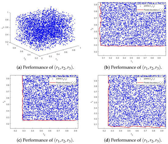
Figure 1. Performance of $(r_1,r_2,r_3)$ and Pareto boundary of $(r_1^{*},r_2^{*})$, $(r_2^{*},r_3^{*})$, $(r_3^{*},r_1^{*})$.

Figure 2 shows the surface of the Pareto boundary, which verifies the relationships between $(r_1^{*},r_2^{*},r_3^{*})$ and $(r_1,r_2,r_3)$ described by (33).

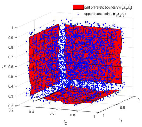
Figure 2. Performance of Pareto boundary $(r_1^{*},r_2^{*},r_3^{*})$.

Figure 3 shows the profile of Brownian motion $W\left(t\right)$, and Figure 4 illustrates the trajectories of $\xi \left(t\right)$, $\eta \left(t\right)$ and $\zeta \left(t\right)$ in System (31) driven by a Brownian motion. Figure 5 illustrates trajectories of $u_1\left(t\right)$, $u_2\left(t\right)$ and $u_3\left(t\right)$, and they represent the investment strategies of government, bank consortium and public, respectively.

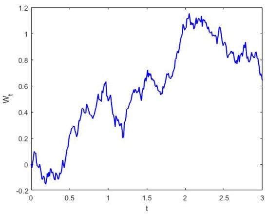
Figure 3. Profiles of Brownian motion.

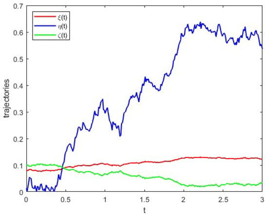
Figure 4. Trajectories of $\xi \left(t\right)$, $\eta \left(t\right)$ and $\zeta \left(t\right)$.

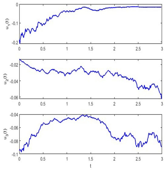
Figure 5. Trajectories of controllers $u_1\left(t\right)$, $u_2\left(t\right)$ and $u_3\left(t\right)$.

6. Conclusions

The non-cooperative game strategy for a nonlinear stochastic time-varying parameter financial system is studied. The proposed non-cooperative game is robust enough to achieve the desired goal of each player. Different from the traditional iterative method, it can be solved by all participants at the same time, and can realize the Nash equilibrium solution. When the value of a parameter in the system changes with time, the entire property changes with time. Finally, a practical example of investment and international capital flow is given to verify the performance of the proposed non-cooperative game strategy design for nonlinear stochastic time-varying parameter systems with continuous fluctuations.

References

- Reny, P.J. Nash equilibrium in discontinuous games. Annu. Rev. Econ. 2020, 12, 439–470. [Google Scholar] [CrossRef]
- Fu, H.F. On the existence of Pareto undominated mixed-strategy Nash equilibrium in normal-form games with infinite actions. Econ. Lett. 2021, 201, 109771. [Google Scholar] [CrossRef]
- Poveda, J.I.; Krstic, M.; Basar, T. Fixed-time Nash equilibrium seeking in time-varying networks. IEEE Trans. Autom. Control 2023, 68, 1954–1969. [Google Scholar] [CrossRef]
- Nash, J. Non-cooperative games. Ann. Math. 1951, 54, 286–295. [Google Scholar] [CrossRef]
- Goldman, A.J.; Shier, D.R. Player aggregation in noncooperative games. J. Res. Natl. Bur. Stand. 1980, 86, 391–396. [Google Scholar] [CrossRef] [PubMed]
- Zhao, C.X.; Hong, S.H.; Li, C.H. Existence of extended Nash equilibriums of nonmonetized noncooperative games. Fixed Point Theory Appl. 2015, 2015, 65. [Google Scholar] [CrossRef]
- Ye, M.J.; Hu, G.Q. Distributed seeking of time-varying Nash equilibrium for non-cooperative games. IEEE Trans. Autom. Control 2015, 60, 3000–3005. [Google Scholar] [CrossRef]
- Aduba, C.; Won, C.H. N-player statistical Nash game control: m-th cost cumulant optimization. IEEE Trans. Autom. Control 2016, 61, 2688–2694. [Google Scholar] [CrossRef]
- Bressan, A.; Nguyen, K.T. Stability of feedback solutions for infinite horizon noncooperative differential games. Dyn. Games Appl. 2018, 8, 42–78. [Google Scholar] [CrossRef]
- Dianetti, J.; Ferrari, G. Nonzero-sum submodular monotone-follower games: Existence and approximation of Nash equilibria. SIAM J. Control Optim. 2020, 58, 1257–1288. [Google Scholar] [CrossRef]
- Zhang, Y.; Chang, S.S.; Chen, T. Existence and generic stability of strong noncooperative equilibria of vector-valued games. Mathematics 2022, 9, 3158. [Google Scholar] [CrossRef]
- Zhang, Y.F.; Liu, F.; Wang, Z.J.; Chen, Y.; Feng, S.L.; Wu, Q.W.; Hou, Y.H. On Nash-Stackelberg-Nash games under decision-dependent uncertainties: Model and equilibrium. Automatica 2022, 142, 110401. [Google Scholar] [CrossRef]
- Setiawan, R.; Salmah; Endrayanto, I.; Indarsih. Analysis of the n-person noncooperative supermodular multiobjective games. Oper. Res. Lett. 2023, 51, 278–284. [Google Scholar] [CrossRef]
- Ma, J.H.; Chen, Y.S. Study for the bifurcation topological structureand the global complicated character of a kind of nonlinear financesystem. Appl. Math. Mech. 2001, 22, 1240–1251. [Google Scholar] [CrossRef]
- Cont, R.; Tankov, P. Financial Modelling with Jump Processes; CRC Press: Boca Raton, FL, USA, 2004. [Google Scholar]
- Wang, L. Dynamic model of stock prices based on technical tradingrules—Part I: The models. IEEE Trans. Fuzzy Syst. 2015, 23, 787–801. [Google Scholar] [CrossRef]
- Wang, L. Dynamical model of stock prices based on technical trading rules—Part II: Analysis of the model. IEEE Trans. Fuzzy Syst. 2015, 23, 1127–1141. [Google Scholar] [CrossRef]
- Wang, L. Dynamic model of stock prices based on technical tradingrules—Part III: Application to Hong Kong stocks. IEEE Trans. Fuzzy Syst. 2015, 23, 1680–1697. [Google Scholar] [CrossRef]
- Stoyanov, J. Stochastic financial models. J. Roy. Stat. Soc. A (Stat. Soc.) 2001, 174, 510–511. [Google Scholar] [CrossRef]
- Chen, B.S.; Chen, W.H.; Wu, H.L. Robust H2/H∞ global linearization filter design for nonlinear stochastic systems. IEEE Trans. Circuits Syst. 2009, 56, 1441–1454. [Google Scholar] [CrossRef]
- Wu, C.F.; Chen, B.S.; Zhang, W. Multiobjective investment policy for a nonlinear stochastic financial system: A fuzzy approach. IEEE Trans. Fuzzy Syst. 2017, 25, 460–474. [Google Scholar] [CrossRef]
- Chen, B.S.; Yeh, C.H. Stochastic noncooperative and cooperative evolutionary game strategies of a population of biological network under natural selection. Bio. Syst. 2017, 162, 90–118. [Google Scholar] [CrossRef] [PubMed]
- Chen, B.S.; Chen, W.Y.; Young, C.T.; Yan, Z. Noncooperative game strategy in cyber-financial systems with Wiener and Poisson random fluctuations: LMIs-constrained MOEA approach. IEEE Trans. Cybern. 2018, 48, 3323–3336. [Google Scholar] [CrossRef] [PubMed]
- Chen, B.S.; Lee, M.Y. Noncooperative and cooperative strategy designs for nonlinear stochastic jump diffusion systems with external disturbance: T-S fuzzy approach. IEEE Trans. Fuzzy Syst. 2020, 28, 2437–2451. [Google Scholar] [CrossRef]
- Tan, C.; Zhang, S.; Wong, W.; Zhang, Z. Feedback stabilization of uncertain networked control systems over delayed and fading channels. IEEE Trans. Control Netw. Syst. 2021, 8, 260–268. [Google Scholar] [CrossRef]
- Tan, C.; Yang, L.; Zhang, F.; Zhang, Z.; Wong, W. Stabilization of discrete time stochastic system with input delay and control dependent noise. Syst. Control Lett. 2019, 123, 62–68. [Google Scholar] [CrossRef]
- Zhang, T.; Deng, F.; Sun, Y.; Shi, P. Fault estimation and fault-tolerant control for linear discrete time-varying stochastic systems. Sci. China Inf. Sci. 2021, 64, 200201. [Google Scholar] [CrossRef]
- Jiang, X.; Zhao, D. Event-triggered fault detection for nonlinear discrete-time switched stochastic systems: A convex function method. Sci. China Inf. Sci. 2021, 64, 200204. [Google Scholar] [CrossRef]
- Boyd, S.; El Ghaoui, L.; Feron, E.; Balakrishnan, V. Linear Matrix Inequalities in System and Control Theory; SIAM: Philadelphia, PA, USA, 1994. [Google Scholar]
- Tan, C.; Yang, L.; Wong, W. Learning based control policy and regret analysis for online quadratic optimization with asymmetric information structure. IEEE Trans. Cybern. 2022, 52, 4797–4810. [Google Scholar] [CrossRef]
- Tan, C.; Zhang, H.; Wong, W. Delay-dependent algebraic Riccati equation to stabilization of networked control systems: Continuous-time case. IEEE Trans. Cybern. 2018, 48, 2783–2794. [Google Scholar] [CrossRef]
Disclaimer/Publisher’s Note: The statements, opinions and data contained in all publications are solely those of the individual author(s) and contributor(s) and not of MDPI and/or the editor(s). MDPI and/or the editor(s) disclaim responsibility for any injury to people or property resulting from any ideas, methods, instructions or products referred to in the content. |
© 2023 by the authors. Licensee MDPI, Basel, Switzerland. This article is an open access article distributed under the terms and conditions of the Creative Commons Attribution (CC BY) license (https://creativecommons.org/licenses/by/4.0/).