Abstract
The a priori procedure was designed as a pre-data procedure whereby researchers could find the sample sizes necessary to ensure that sample statistics to be obtained are within particular distances of corresponding population parameters with known probabilities. Researchers specify desired precisions (distances of sample statistics from corresponding population parameters) and desired confidences (probabilities of being within desired distances), and this procedure provides necessary sample sizes to meet precision and confidence specifications. Although the a priori procedure has been devised for a variety of experimental paradigms, these have all been simple. The present article constitutes its extension to analysis of variance models. A fortunate side effect of the equations to be proposed is an improvement in efficiency even for a paradigm that fits a previously published article.
Keywords:
the a priori procedure; required sample size; contrasts; analysis of variance model; confidence; precision MSC:
62F10; 62J05
1. Extending the A Priori Procedure to One-Way Analysis of Variance under Normality
Previously, Trafimow and colleagues have proposed the a priori procedure (APP; e.g., [1,2,3]), which invokes a substantial philosophical change from previous inferential statistical procedures. Instead of collecting data and then performing inferential work post-data, the APP features pre-data calculations. The researcher specifies a desired level of precision and a desired level of confidence, and an APP equation (or program) returns the sample size needed to meet both specifications. Consider a simple example from [1] involving a single group, under the usual assumption of a normally distributed population from which the sample was drawn, where the researcher intends to compute the sample mean and use it as an estimate of the population mean. Suppose that the researcher wishes to have 95% confidence (a 95% probability) of obtaining a sample mean within one-tenth of a standard deviation from the population mean. Trafimow in [1] provides the equation under the simplifying assumption that the population variance is known:
where n is the sample size needed to meet specifications for precision and confidence, f is the desired level of precision in terms of a fraction of a standard deviation (e.g., one-tenth of a standard deviation or 0.10), c is the given confidence level (e.g., ), and is the z-score that corresponds to a desired level of confidence (e.g., the z-score of 1.96 corresponds to 95% confidence). Continuing with the example, the sample size needed to meet specifications, using Equation (1), is . Thus, the researcher needs to collect 385 participants to have a 95% probability of obtaining a sample mean within 0.10 of a standard deviation of the population mean.
It is important not to confuse the APP with power analysis as these two procedures are associated with different goals. In power analysis, the goal is to find out how many participants are needed to have a particular probability of obtaining a statistically significant finding, given a specified effect size. For example, a researcher might wish to have 80% power to detect a “medium” effect size of 0.50. Using power analysis with this example, the researcher would conclude that it is necessary to have a sample size of 31 to meet specifications for power and effect size. There are two crucial points of difference between power analysis and the APP. First, power analysis is influenced by the assumed effect size, whereas the APP is not. Second, the APP is influenced by the desired degree of precision, whereas power analysis is not. To dramatize the effects of these two points of difference, contrast the power analysis recommendation of 31 participants and the APP recommendation of 385 participants. Alternatively, the power analysis recommendation of 31 participants results in a precision level of only 0.35, which Trafimow (2017) [2] termed “poor” precision. Whatever dissimilarities the reader prefers to emphasize, the conclusion remains that the APP is different from power analysis.
This paper is organized as follows. In Section 2, a previous APP to handle any number of k means was introduced. The main result, minimum sample size required for estimating the mean vector in ANOVA models, is derived in Section 3. For an illustration of the main results, an online calculator and some results in tables and figures are given in Section 4. A simulation study and real data examples are given in Section 5 and the conclusion and discussion are listed in Section 6.
2. Previous APP Advances
Trafimow and MacDonald [2] expanded the APP to handle any number of means (k means):
where symbolizes the cumulative distribution function of the standard normal distribution, f is the specified precision, and
More recently, Trafimow et al. [3] expanded the APP to render possible for researchers to find the sample sizes needed to meet specifications for precision and confidence pertaining to differences in means in matched or independent samples. In both cases, making a more realistic assumption than in Equation (1), that the population variance is not known, the APP uses inequalities, rather than equations. Consequently, the researcher must perform an iterative process to find the lowest value for n where the inequalities remain true. In the case of matched samples, the same participants are in both groups and so the total sample size remains at n, as Inequality (3) shows:
where is the critical t-score with degrees of freedom, analogous to the use of the z-score from Equation (1).
Alternatively, if there are independent samples, there is no guarantee that the sample sizes will be equal. Trafimow et al. (2020) [3] designate that there are n participants in the smaller group and m participants in the larger group, where . Using ℓ, Inequality (4) follows (see Trafimow et al. 2020 [3] for derivation).
where is the critical t-score that corresponds to the level of confidence level and degrees of freedom in which is rounded to the nearest upper integer. If the researcher has equal sample sizes, Equation (4) reduces to Equation (5):
3. Expansion to Multiple Contrasts
Although Inequalities (3)–(5) are undeniably useful extensions of the APP, they are limited in the sense that many researchers perform more complex designs and are concerned with multiple contrasts. For example, a social psychologist might perform a design with participants randomly assigned to each of the four cells of the design. In this case, there are many possible contrasts, including six possible contrasts between sets of two means. Or researchers sometimes use yet more complex designs. It would be a useful APP expansion to derive a procedure whereby researchers could determine the sample size needed to meet specifications for precision and confidence covering all possible contrasts regardless of the complexity of the design. Our goal is to derive this APP expansion.
3.1. Estimation of Parameters in the One-Way ANOVA Model
In statistics, one-way analysis of variance (abbreviated one-way ANOVA) is a technique that can be used to compare means of two or more samples, see Rencher and Schaalje (2008) [4], Bogartz (1994) [5], Lindman (2012) [6], Scheffe (1999) [7], and MuCulloco (2001) [8]. The one-way ANOVA (effects) model can be expressed as follows:
with the mean effect model
where k is the number of treatment groups, is the jth observed value for the ith treatment group, is the number of observations in the ith treatment group, is the mean for the ith treatment group, is the grand mean and is the ith treatment group effect, a deviation from the grand mean. If , then the model in Equations (6) or (7) is called the balanced model. Assumptions for ANOVA models are that random errors ’s are independent and identically distributed normal random variables with mean 0 and constant variance . The unknown parameters of the models are , ’s and .
Note that the ANOVA model in Equation (6) can be written as a linear model of the form
where and is the identity matrix of order n, is the column vector of all n observations, X is the design matrix of order and is column vector of parameters , , …, . The least square estimators (also the best unbiased estimators) of parameters, with constraint , are
respectively, where is the sample mean for the ith treatment group and is the grand sample mean.
3.2. A Priori Procedures Applied for One-Way ANOVA Models
For estimation of k means , …, , the F-distribution with numerator degrees of freedom k and denominator degrees of freedom is applied. See Appendix A for details. Let and, for , be the critical point such that . Note that for . We have
which is equivalent to
Therefore, without loss of generality, our APP is applied to finding the minimum m based on Equation (10). Specifically, for a given precision level f and a confidence level c, the required treatment group size m can be obtained by solving
where is the inverse of the distribution function of the F-distribution with degrees of freedom k and . Details are given in Table 1.

Table 1.
Required group sizes m needed for each of k means, for given confidence level , and precision when there exist groups. Here is the number of observations for each group given in [2].
For testing hypothesis or , the F-distribution with numerator degrees of freedom and denominator degrees of freedom is applied and the required m can be obtained similarly. Note that this testing hypothesis is equivalent to the estimation of ’s with the constraint or ’s with the constraint . The details are given in Table 2.

Table 2.
Required sample sizes n, for each of k means (ANOVA models), for given confidence level , and precision when there exist groups.
Remark 1.
- (i)
- Since F test is used in two-way or multi-way ANOVA models for testing the main effects and their interactions, we can use the similar method as in Equations (10) and (11) by adjusting degrees of freedoms k and . Therefore, the required sample size n can be obtained from our online calculator given in next section.
- (ii)
- For our ANOVA model in Equation (8), we focus only on the estimation of parameters with the minimum required sample size. To study the robustness of estimators or the shrinkage estimation of in high-dimensional generalized linear models, we suggest Roozbeh et al. (2023) [9], Yüzbaşı et al. (2020) [10], and Yüzbaşı et al. (2021) [11] for interested readers.
- (iii)
- For ANOVA models with skew normal random errors, our APP procedure can be applied using non-central skew F distributions, which are extensions of the standard F distribution used in this paper; see Azzalini (2013) [12], Ye et al. (2023) [13], and Ye et al. (2023) [14] for more details.
4. Implications
The foregoing mathematics suggest implications. These include implications pertaining to the issue of having all the sample means for all groups fall within specifications for precision and confidence and contrasts. The subsequent subsections address these.
4.1. Having Means for All Groups Fall within Specifications
Table 1 and Figure 1 and Figure 2 provide direct implications, and Figure 3 compares the present technique against that provided by Trafimow and MacDonald (2017) [2]. To compute the required sample size n for ANOVA models, we provide an online calculator at https://apprealization.shinyapps.io/Anova/ (accessed on 26 December 2023).

Figure 1.
The sample size per group ranges along the vertical axis as a function of the desired degree of precision along the horizontal axis and whether the desired confidence is at the 95% level (top curve) or 90% level (bottom curve).

Figure 2.
The sample size per group ranges along the vertical axis as a function of the number of groups along the horizontal axis (3 to 10) and whether the desired confidence is at the 95% level (top curve) or 90% level (bottom curve).

Figure 3.
The sample size per group ranges along the vertical axis as a function of the desired degree of precision along the horizontal axis based on the Trafimow and MacDonald (2017) [2] procedure (top curve) or new procedure (bottom curve).
We consider the implications of each figure below. Figure 1 presents two panels, featuring where there are three groups or four groups. In both panels, the required sample size per group ranges along the vertical axis as a function of precision along the horizontal axis and with separate curves representing a researcher who desires 95% confidence (top curve) or 90% confidence (bottom curve). Commencing with the panel featuring three groups, more confidence implies a larger sample size. In addition, as precision becomes less stringent, the sample size necessary to meet the criterion decreases. There is an important interaction between precision and confidence in that the effect of precision is more dramatic at 95% confidence than at 90% confidence. The panel featuring four groups suggests similar implications but with a potentially misleading aspect. Specifically, sample sizes in this panel tend to be smaller than corresponding sample sizes in the panel featuring three groups, which may seem to imply that more groups are better than fewer groups. At the within group level, this implication is true. But at the total group level, where the total sample size is a function of all groups, the implication is not true as the total sample size is larger when there are more groups than when there are fewer groups.
In Figure 2, the required sample size per group ranges along the vertical axis as a function of the number of groups along the horizontal axis. Again, there are two curves in each panel, with each curve representing a different level of confidence. Although the same lessons illustrated in Figure 1 come across in Figure 2 as well, Figure 2 does a better job than Figure 1 of illustrating the effect of the number of groups. When the precision criterion is stringent, at 0.10 in the first panel, the number of groups has what might be considered to be an important effect on necessary sample sizes, though as groups continue to be added, this effect diminishes. But when the precision criterion is set at the less stringent value of 0.20 in the second panel, varying the number of groups has less of an influence and necessary sample sizes are generally lower. However, remember that the effects illustrated in Figure 2, as in Figure 1, are on the sample size per group. As the number of groups increases, the total sample size, across all groups, increases too.
In contrast to Figure 1 and Figure 2, which were designed to facilitate understanding the sample size implications of the new technique, Figure 3 was designed to answer what otherwise would be an inconvenient question. Specifically, given that Trafimow and MacDonald (2017) [2] already have established a technique for finding the sample sizes needed to meet various specifications for precision and confidence pertaining to all means, why do we need another technique? There are two answers. One answer is that the present mathematics increase important capabilities, as the subsequent subsections explain. The second answer, to be addressed now, is that the present technique is more efficient than the old one proposed by Trafimow and MacDonald (2017) [2].
In Figure 3, like Figure 1, required sample size per group again ranges along the vertical axis as a function of precision along the horizontal axis. But this time the top curve represents the old technique Trafimow and MacDonald (2017) [2], whereas the bottom curve represents the new technique advocated here, based on the mathematics presented in the foregoing section. One panel assumes the researcher desires 95% confidence, whereas the other panel assumes the researcher desires 90% confidence. Starting with the 95% confidence panel, we see the typical effect of decreasing sample sizes as precision becomes less stringent. It is important, however, not only that the new technique provides an obvious sample size savings relative to the old method but also that the extent of the savings is magnified under stringent precision. The 90% confidence panel illustrates similar lessons but to a lesser extent than the 95% panel.
There is one additional point of comparison between the old and new techniques. In the old technique, as there are more groups, the required total sample size increases, as is true with the new technique too. However, if we consider the required sample size per group, as a function of the number of groups, there is an important change. Under the old technique, more groups imply a larger required sample size per group, but under the new technique, more groups imply a smaller sample size per group.
4.2. Contrasts between Means
One limitation of the technique provided by Trafimow and MacDonald (2017) [2] is that there is no way to find necessary sample sizes to meet specifications for precision and confidence pertaining to differences in means in different conditions. For example, suppose it is important for the researcher to obtain a good estimate of the difference in population means based on samples in Group 1 versus Group 4. The new technique renders possible the determination of the necessary sample sizes.
Table 2 and Figure 4 illustrate the implications. Like Figure 1, the sample size per group ranges along the vertical axis as a function of precision ranging along the horizontal axis, with curves representing 95% confidence or 90% confidence. Also, like Figure 1, there are panels for studies involving three groups and four groups. Further, the lessons are similar to the lessons illustrated by Figure 1 that need not be reiterated here. But there is an additional issue that results from comparing Figure 4 to Figure 1. Specifically, the sample size requirements are slightly larger in Figure 4 than in Figure 1. For example, under precision of 0.10 and 95% confidence, when there are three groups, the sample size requirement per group is 263 in Figure 1, but it is 301 in Figure 4, for a difference of 38. This difference diminishes with less stringent precision or less stringent confidence. If precision is set at the more liberal level of 0.2, the sample size requirement is 67 in Figure 1 and 76 in Figure 2, for a difference of only 9. Or, if we keep precision at 0.10 but drop the confidence specification to 90%, the sample size requirement is 210 in Figure 1, but it is 232 in Figure 2, for a difference of 22—still less than the difference of 38 at 95% confidence.

Figure 4.
The sample size (ANOVA models) ranges along the vertical axis as a function of the desired degree of precision along the horizontal axis and whether the desired confidence is at the 95% level (top curve) or 90% level(bottom curve).
To gain an idea of the importance, or lack of importance, of the number of groups, consider Figure 5. In Figure 5, the sample size per group ranges along the vertical axis as a function of the number of groups along the horizontal axis, with curves for 95% confidence (top curve) or 90% confidence (bottom curve). Like Figure 2, the two panels indicate more stringent precision (0.10) or less stringent precision (0.20). The lessons illustrated by Figure 5 echo the lessons illustrated by Figure 2 but with the additional demonstration that larger sample sizes are needed in Figure 5 than in Figure 2.

Figure 5.
The sample size (ANOVA models) ranges along the vertical axis as a function of the number of groups along the horizontal axis (2 to 10) and whether the desired confidence is at the 95% level (top curve) or 90% level (bottom curve).
5. Simulation and Real-Data Example
In this section, we perform a simulation study and also give a real-data example to evaluate the performance of the proposed APP. To compute the required minimum sample size n for estimating the mean vector , we can use the online calculator provided in above section for given f, c and k.
Simulation: Using the Monte Carlo methods, we provide the coverage rate (cr) corresponding to each sample size based on M = 10,000 runs (samples) in Table 3. The coverage rate (cr) is the percentage of the population mean falling into the confidence region of the specified confidence level among these 10,000 samples.

Table 3.
For and , the required sample size and coverage rate (cr).
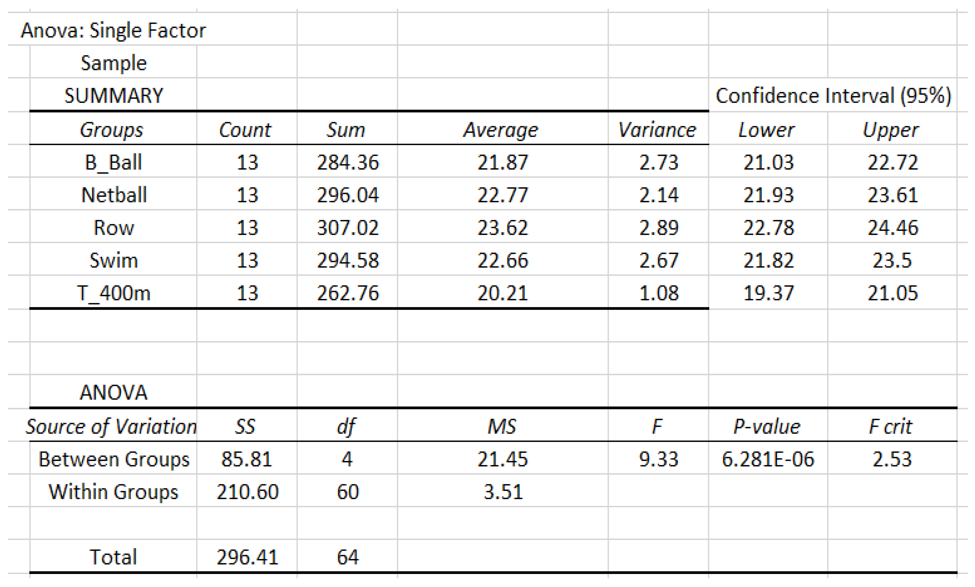
Real-data examples: The data set was obtained from R package named DAAG. The following page explains the details and reference of the data: https://pmagunia.com/dataset/r-dataset-package-daag-ais (accessed on 26 December 2023).
These data, called BMI data, were collected in a study of how data for various characteristics of the blood varied with sport body size and sex of the athlete. We will use the body mass index (BMI) data of athletes in five sports (B_Ball, Netball, Row, Swim, and T_400m) to set up our ANOVA model.
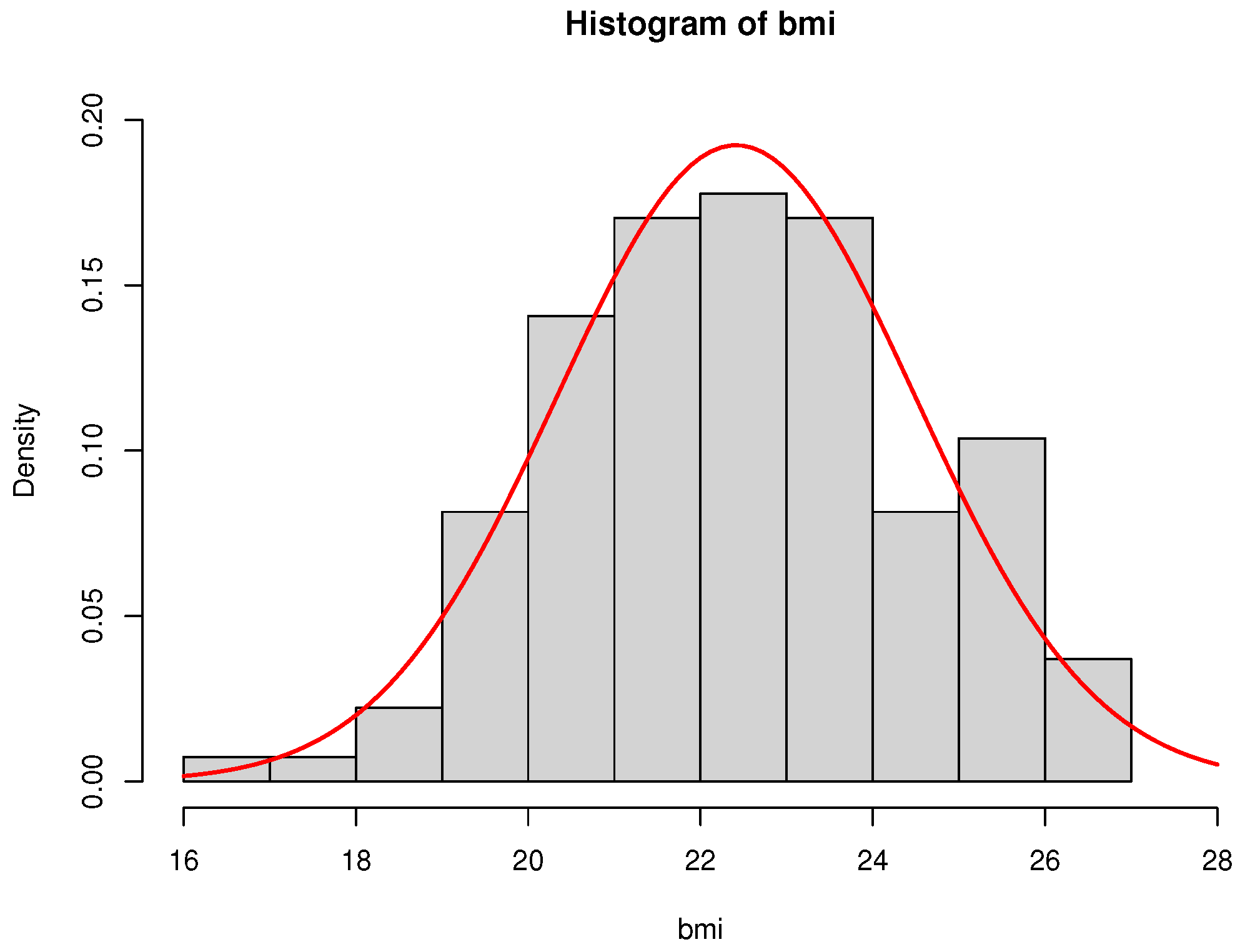
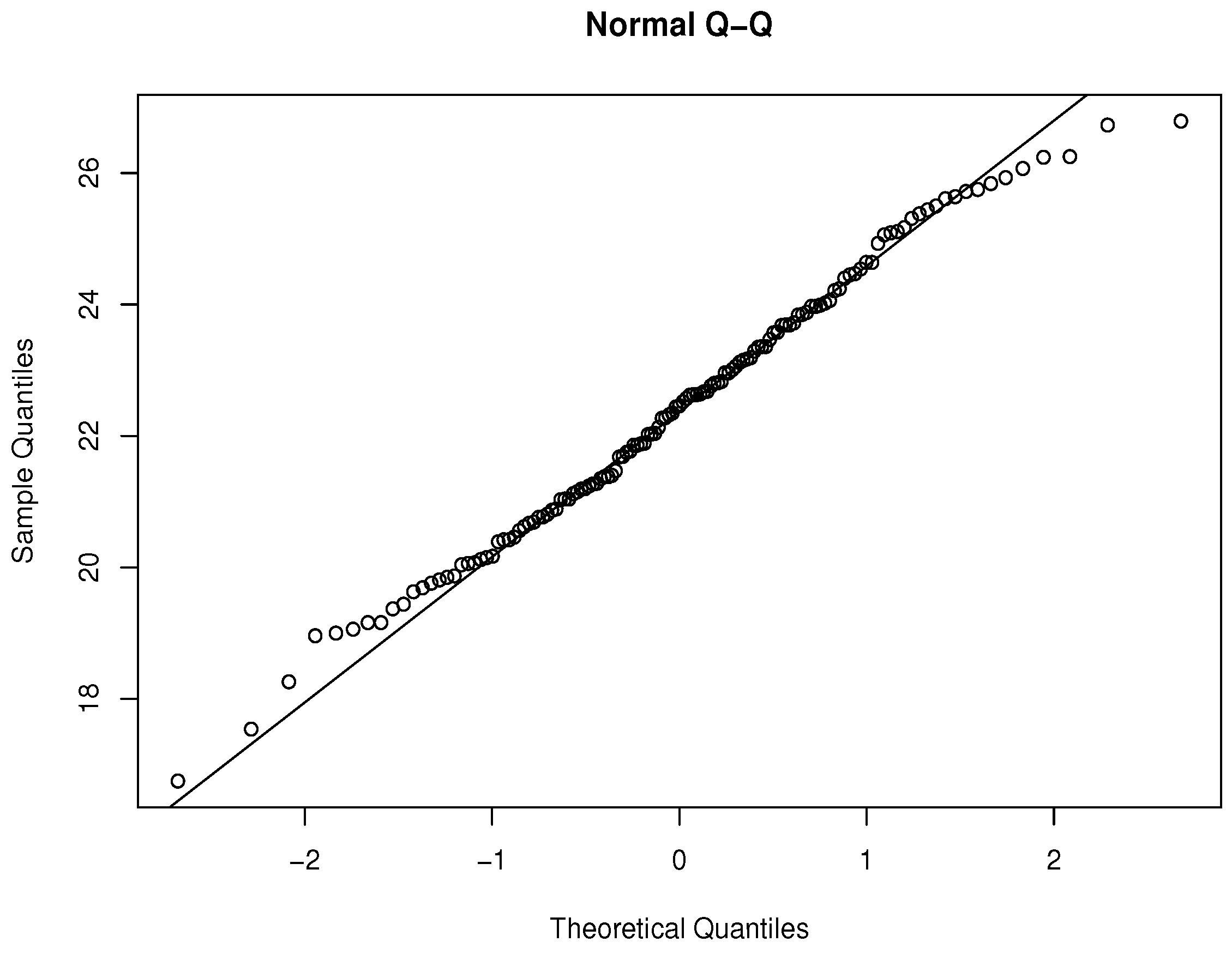
First, we need to check the normality assumptions of the data set which are given in Figure 6 (histogram) and Figure 7 (the QQ plot), respectively.
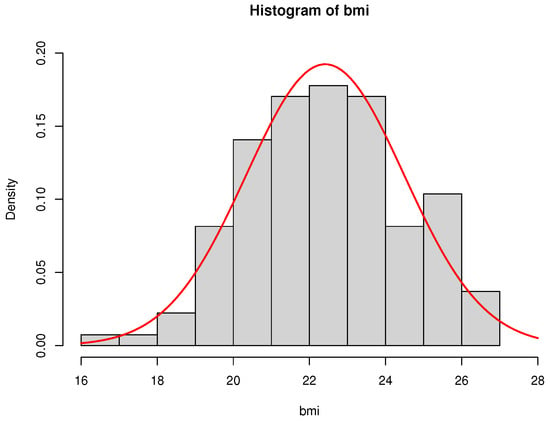
Figure 6.
Histogram and its fitted normal density curve of BMI data.
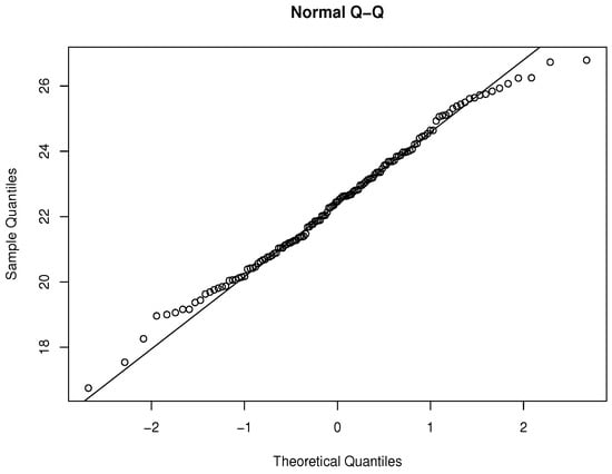
Figure 7.
Q-Q plot of BMI data.
It is easy to say that the normality assumptions are valid, which are also supported by goodness of fit tests (e.g., Shapiro–Wilk Test).
Example 1.

The BMI data are based on the classification of gender (female and male). The details of the analysis are given in Figure 8.

Figure 8.
Data analysis of population based on the classification of gender.
Now, we apply our APP method with , and . The total required sample size is . Then we draw two samples of size from the population (35 from female BMI data and another 35 from male BMI data). The summaries of samples are given in Figure 9.

Figure 9.
Data analysis of sample based on the classification of gender.
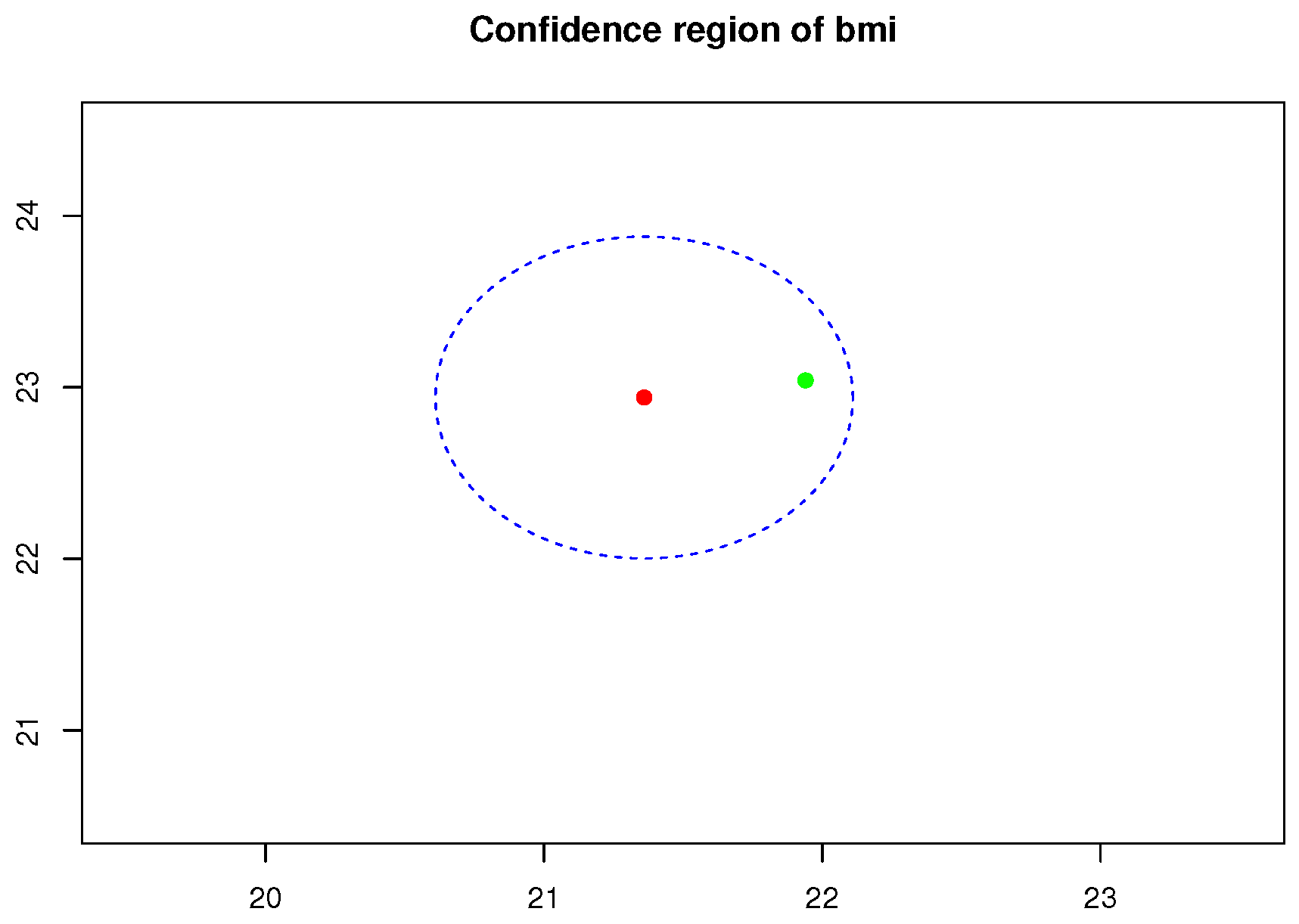
The confidence region of BMI data, using Equation (A7), of population mean vector for given is given in Figure 10.
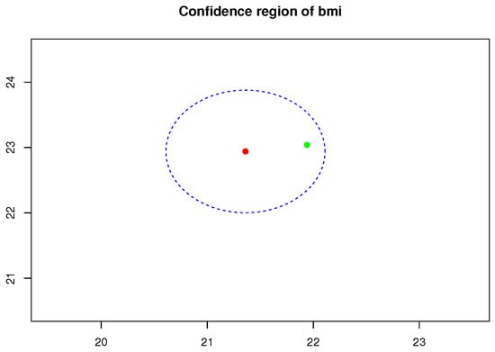
Figure 10.
Confidence region of population mean vector (green point) enclosed by blue dashed circle for given and and the corresponding point estimator (red point).
Example 2.
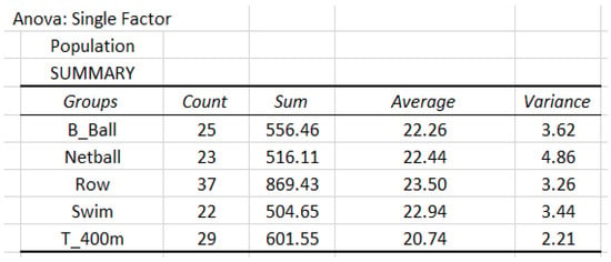
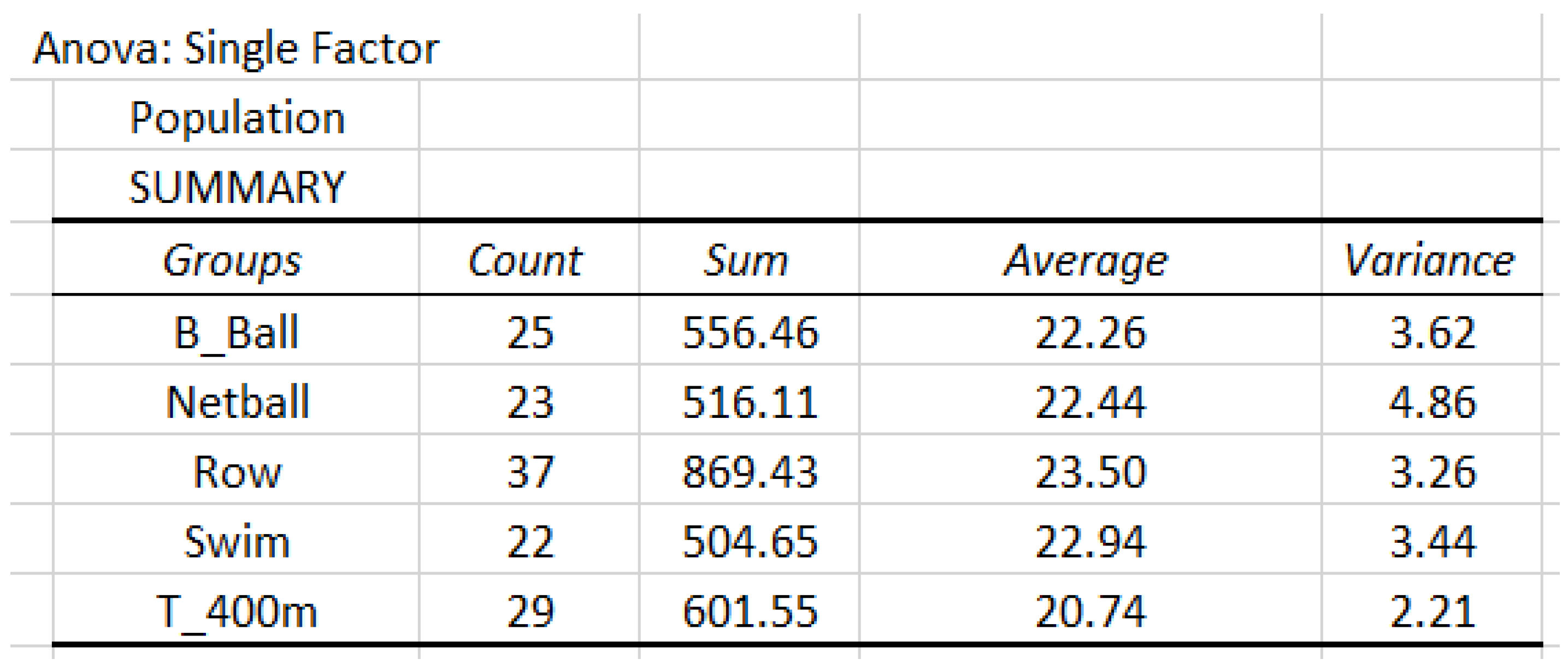
The BMI data are based on the classification of five sports (B_Ball, Netball, Row, Swim, and T_400m). The details are give in Figure 11.

Figure 11.
Data analysis of population based on the classification of sports.
Now, we apply our APP method with , and . The total required sample size is . Then we draw samples of size of BMI data in each sport from the population. The details of analysis are given in Figure 12.
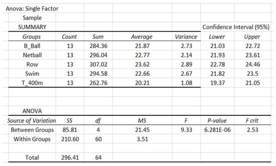
Figure 12.
Data analysis of sample based on the classification of sports.
6. Conclusions and Discussion
The present work expands the APP to a new domain: ANOVA paradigms. Even if the goal is merely to determine the sample sizes needed for obtaining k means within specifications for precision and confidence, the present procedure is more efficient than the previous procedure by Trafimow and MacDonald (2017) [2]. And the extra efficiency is particularly evident under stringent criteria for precision (e.g., ) and confidence (e.g., 95%). We hope and expect that the present work will aid researchers in obtaining sample means and contrasts that they can trust will be good estimates of population ones.
Before collecting data, it is desirable for researchers to have a way to estimate the necessary sample size needed to meet specifications for precision and confidence. The APP provides that, and we have already discussed some APP advances. One such advance is the application to multiple group or ANOVA designs, as opposed to being restricted to two-group designs. Although Trafimow and MacDonald (2017) [2] had previously suggested a way to handle such designs, it is possible to improve on that method. The present proposal adds to the literature for two reasons. The current method is considerably more efficient than the previous one, especially when precision criteria are stringent. Secondly, we provide a link to an online calculator so even mathematically unsophisticated researchers can perform the calculations.
Even though our present proposal was designed for one-way ANOVA designs, sometimes researchers have two-way designs, three-way designs and so on, so they can assess main effects and interactions. However, because our concern is pre-data, with estimating necessary sample sizes to meet specifications for precision and confidence, the present procedure is agnostic about how researchers plan to analyze the data after collecting it.
Since F tests are also used in two-way or multi-way ANOVA models for testing the main effects and their interactions, we can use the similar method as in Equations (10) and (11) by adjusting degrees of freedom k and . Thus, any multidimensional design can be converted into a one-way ANOVA by simple multiplication. For example, suppose a researcher has a design with and , the two-way ANOVA model with interaction. From the point of view of the present proposal, this is equivalent to a one-way design using F distribution with fixed-numerator degrees of freedom and denominator degree of freedom . Thus, to use the link to the calculator, one could simply specify the number of groups in the numerator degrees of freedom to find the total requires sample size , where m is the number of replicates in the treatment with level i of the first factor and level j of the second factor, and . If we use and , the total required sample size is so that . Currently, we are applying our APP methods to multidimensional ANOVA models with real-data applications; see Zhu et al. (2018) [15], Zhu et al. (2021) [16], and Zhu et al. (2022) [17] to name a few. More generally, the present proposal can be generalized to a design with any number of dimensions to find the necessary sample size to meet specifications for precision and confidence.
Author Contributions
Conceptualization, T.W. and D.T.; methodology, L.H. and T.W.; software, L.H.; validation, L.H., T.W., D.T. and S.T.B.C.; formal analysis, L.H.; investigation, L.H., T.W., D.T. and S.T.B.C.; resources, L.H., T.W., D.T. and S.T.B.C.; data curation, L.H.; writing—original draft preparation, L.H. and T.W.; writing—review and editing, L.H., T.W., D.T. and S.T.B.C.; visualization, L.H., T.W., D.T. and S.T.B.C.; supervision, T.W., D.T. and S.T.B.C.; project administration, T.W. and D.T. All authors have read and agreed to the published version of the manuscript.
Funding
This research received no external funding.
Data Availability Statement
The data in our examples are from published online data: https://pmagunia.com/dataset/r-dataset-package-daag-ais (accessed on 26 December 2023).
Acknowledgments
The authors would like to thank all anonymous reviewers for their valuable suggestions and comments, which improved the quality of the manuscript.
Conflicts of Interest
The authors declare no conflict of interest.
Appendix A
We will use the linear model of the form given in Equation (8) to illustrate our A Priori Procedure:
where . For example, if and , then X is a matrix, and so that the model is shown as follows:
Note that for any estimable function with full column rank p of A, the best unbiased estimator of is where is given in Equation (8). The properties of are listed as below:
- (i)
- , the p-dimensional normal distribution with mean , and covariance , where is a generalized inverse of .
- (ii)
- is invariant to the choice of so that we can select the easiest
We can construct a confidence region for with confidence level c and precision f. The confidence region is given by
Now, we will consider the following two special cases of A discussed in the paper under the section “A Priori Procedures Applied for One-Way ANOVA Models”.
- (i)
- For estimation of k means , we choose , an matrix with rank . It is easy to check that so that the required m can be obtained from Equation (A6).
- (ii)
- For the estimation of ’s with constraint , we choose the
References
- Trafimow, D. Using the coefficient of confidence to make the philosophical switch from a posteriori to a priori inferential statistics. Educ. Psychol. Meas. 2017, 77, 831–854. [Google Scholar] [CrossRef] [PubMed]
- Trafimow, D.; MacDonald, J.A. Performing inferential statistics prior to data collection. Educ. Psychol. Meas. 2017, 77, 204–219. [Google Scholar] [CrossRef] [PubMed]
- Trafimow, D.; Wang, C.; Wang, T. Making the a priori procedure (APP) work for differences between means. Educ. Psychol. Meas. 2020, 80, 186–198. [Google Scholar] [CrossRef] [PubMed]
- Rencher, A.C.; Schaalje, G.B. Linear Models in Statistics; John Wiley & Sons: Hoboken, NJ, USA, 2008. [Google Scholar]
- Bogartz, R.S. An Introduction to the Analysis of Variance; Praeger Publishers/Greenwood Publishing Group: New York, NY, USA, 1994. [Google Scholar]
- Lindman, H.R. Analysis of Variance in Experimental Design; Springer Science & Business Media: New York, NY, USA, 2012. [Google Scholar]
- Scheffe, H. The Analysis of Variance; John Wiley & Sons: New York, NY, USA, 1999. [Google Scholar]
- McCulloch, C.E.; Searle, R. Generalized, Linear, and Mixed Models; John Wiley & Sons: New York, NY, USA, 2001. [Google Scholar]
- Roozbeh, M.; Maanavi, M.; Mohamed, N.A. A robust counterpart approach for the ridge estimator to tackle outlier effect in restricted multicollinear regression models. J. Stat. Comput. Simul. 2023, 1–18. [Google Scholar] [CrossRef]
- Yüzbaşı, B.; Arashi, M.; Ejaz, A.S. Shrinkage Estimation Strategies in Generalised Ridge Regression Models: Low/High-Dimension Regime. Int. Stat. Rev. 2020, 88, 229–251. [Google Scholar] [CrossRef]
- Yüzbaşı, B.; Arashi, M.; Akdeniz, F. Penalized regression via the restricted bridge estimator. Soft Comput. 2021, 25, 8401–8416. [Google Scholar] [CrossRef]
- Azzalini, A. The Skew-Normal and Related Families; Cambridge University Press: Cambridge, UK, 2013. [Google Scholar]
- Ye, R.; Du, W.; Lu, Y. Bootstrap inference for skew-normal unbalanced heteroscedastic one-way classification random effects model. J. Stat. Comput. Simul. 2023, 93, 2672–2702. [Google Scholar] [CrossRef]
- Ye, R.; Du, W.; Lu, Y. Bootstrap inference for unbalanced one-way classification model with skew-normal random effects. Commun. Stat.-Simul. Comput. 2023, 1–22. [Google Scholar] [CrossRef]
- Zhu, Y.; Phillip, L.; Srijana, D.; Robert, S.; Tom, W.; Zhang, J. Evaluation of commercial Upland (Gossypium hirsutum) and Pima (G. barbadense) cotton cultivars, advanced breeding lines and glandless cotton for resistance to Alternaria leaf spot (Alternaria alternata) under field conditions. Euphytica 2018, 214, 147. [Google Scholar] [CrossRef]
- Zhu, Y.; Abdelraheem, A.; Wheeler, T.A.; Dever, J.K.; Wedegaertner, T.; Hake, K.D.; Zhang, J. Interactions between cotton genotypes and Fusarium wilt race 4 isolates from Texas and resistance evaluation in cotton. Crop Sci. 2021, 61, 1809–1825. [Google Scholar] [CrossRef]
- Zhu, Y.; Heather, E.; Terry, A.B.; Jane, D.; Derek, W.; Kater, H.; Tom, W.; Zhang, J. Effect of growth stage, cultivar, and root wounding on disease development in cotton caused by Fusarium wilt race 4 (Fusarium oxysporum f. sp. vasinfectum). Crop Sci. 2022, 63, 101–114. [Google Scholar] [CrossRef]
Disclaimer/Publisher’s Note: The statements, opinions and data contained in all publications are solely those of the individual author(s) and contributor(s) and not of MDPI and/or the editor(s). MDPI and/or the editor(s) disclaim responsibility for any injury to people or property resulting from any ideas, methods, instructions or products referred to in the content. |
© 2023 by the authors. Licensee MDPI, Basel, Switzerland. This article is an open access article distributed under the terms and conditions of the Creative Commons Attribution (CC BY) license (https://creativecommons.org/licenses/by/4.0/).


