Dynamics of a Prey–Predator Model with Group Defense for Prey, Cooperative Hunting for Predator, and Lévy Jump

Abstract

A stochastic predator–prey system with group cooperative behavior, white noise, and Lévy noise is considered. In group cooperation, we introduce the Holling IV interaction term to reflect group defense of prey, and cooperative hunting to reflect group attack of predator. Firstly, it is proved that the system has a globally unique positive solution. Secondly, we obtain the conditions of persistence and extinction of the system in the sense of time average. Under the condition that the environment does not change dramatically, the intensity of cooperative hunting and group defense needs to meet certain conditions to make both predators and preys persist. In addition, considering the system without Lévy jump, it is proved that the system has a stationary distribution. Finally, the validity of the theoretical results is verified by numerical simulation.

1. Introduction

The predator–prey model is one of the most interesting and important topics in mathematical ecology, and has attracted many mathematicians and ecologists to study it. In the mid-20th century, Leslie and Gower [1,2] proposed a Leslie–Gower-type predator–prey model, which is characterized by the decrease in the number of predators being inversely proportional to its per capita preference for food availability. Considering that the number of predators was limited by the most important food, AzizAlaoui and Okiye [3] proposed the modified Leslie–Gower-type model. As far as we know, there are many articles on the Leslie–Gower model, most of which are deterministic equations. There are not many studies on Leslie–Gower with white noise and Lévy noise, and almost no research on the Leslie–Gower model with cooperative hunting and group defense functions.

In the predator–prey model, the predation rate intuitively reflects the relationship between the two populations. Scholars have proposed a series of functional responses to describe the predation rate [4,5,6,7,8]. Ali et al. [9] numerically studied the effects of nonlinear reaction–diffusion equations on the dynamics of prey–predator interactions. In nature, cooperation between species of the same species is common, and many scholars have introduced cooperation items into the modeling of functional responses for predation rates. Among them, there is cooperative hunting, such as lions hunting faster animals [10,11] and wolves hunting collectively against animals larger than themselves [12], and many scholars have studied the significance of hunting cooperation [13,14]. Chow and Jang [15] studied a predator–prey system with $\frac{ay}{1+ay}$ as the cooperative hunting term, where a is the coefficient related to cooperation strength. The results show that large-scale cooperative hunting may promote the persistence of predators. If there is no cooperation, predators will become extinct. Of course, species at the bottom of the food chain usually carry out group defense through mass reproduction. Andrews [16] proposed the so-called Monod–Haldane function and used it to model the inhibitory effect at high concentrations. Then, Sokol and Howell [17] proposed a simplified Monod–Haldane function of the form $\frac{K_{1}S}{K_2+S^2}$. After that, Shen [18] used a simple Holling IV to describe the group defense of prey for research. Bai [19] studied the global dynamics of a predator–prey system with cooperative hunting, and found that cooperative hunting is beneficial to the coexistence of prey and predator. Du [20] considered the cooperative hunting and group defense of the system without random perturbations, and the effect of predator cooperative hunting and predation aggregation on the stability of coexistence and system dynamics. Recently, many scholars have studied the models with group defense [21,22,23,24].

Inspired by the above articles, we add the Holling IV type function and cooperative hunting term into the Leslie–Gower model to show the cooperation of prey and predator.

$$\left\{\begin{array}{cc}\hfill \mathrm{d}x\left(t\right)=& x\left(t\right)\left[a-bx\left(t\right)-\frac{q{y}^2\left(t\right)}{\left(m+y\left(t\right)\right)\left(c+x^2\left(t\right)\right)}\right]\mathrm{d}t,\hfill \\ \hfill \mathrm{d}y\left(t\right)=& y\left(t\right)\left[\delta -\frac{hy\left(t\right)}{l+x\left(t\right)}\right]\mathrm{d}t,\hfill \end{array}\right.$$

(1)

with initial values $x\left(0\right)=x_0$ and $y\left(0\right)=y_0$. $x\left(t\right)$ and $y\left(t\right)$ denote the number of prey and predators at time t. It should be noted that $a,\delta ,b,q,m,c,h$, and l are all positive numbers. The parameters a and $\delta$ are the growth rate of the prey and the predator, respectively. b represents the intensity of competition between individuals of the prey. l describes the degree of protection provided by the environment to the predator. h denotes the maximum per capita reduction rate of the prey. $\frac{x\left(t\right)}{c+x^2\left(t\right)}$ is the simplified Holling IV functional response function, where c describes the degree of group defense. $\frac{qy\left(t\right)}{m+y\left(t\right)}$ is the cooperative hunting term, where q and m are cooperative coefficients, reflecting the intensity of cooperative hunting between predators.

What we know is that there are endless noise disturbances in nature. In the past, random biological models [25,26,27,28] have been a hot topic for biologists. In the study of stochastic interference, there are both white noise [29,30] and Lévy jump [31,32] considering sudden environmental disturbance. Random perturbations described by Brownian motion describe continuous effects, and Lévy jumps are considered to describe sudden and violent environmental changes well. Therefore, considering both white noise and Lévy noise is more realistic, so we obtain the following stochastic model:

$$\left\{\begin{array}{cc}\hfill \mathrm{d}x\left(t\right)=& x\left(t\right)\left[a-bx\left(t\right)-\frac{q{y}^2\left(t\right)}{(m+y\left(t\right))(c+x^2\left(t\right))}\right]\mathrm{d}t\hfill \\ \hfill & +{\sigma }_{1}x\left(t\right)\mathrm{d}{B}_1\left(t\right)+{\int }_{\mathsf{\Gamma }}x\left(t^{-}\right){\gamma }_1\left(u\right)\tilde{\mathrm{N}}(\mathrm{d}u,\mathrm{d}t),\hfill \\ \hfill \mathrm{d}y\left(t\right)=& y\left(t\right)\left[\delta -\frac{hy\left(t\right)}{l+x\left(t\right)}\right]\mathrm{d}t+{\sigma }_{2}y\left(t\right)\mathrm{d}{B}_2\left(t\right)\hfill \\ \hfill & +{\int }_{\mathsf{\Gamma }}y\left(t^{-}\right){\gamma }_2\left(u\right)\tilde{\mathrm{N}}(\mathrm{d}u,\mathrm{d}t),\hfill \end{array}\right.$$

(2)

where $B_1\left(t\right)$ and $B_2\left(t\right)$ are mutually independent standard Brownian motions, and $x\left(t^{-}\right),$$y\left(t^{-}\right)$ denote the left limits of $x\left(t\right)$ and $y\left(t\right)$. $\mathrm{N}(\mathrm{d}u,\mathrm{d}t)$ is a Poisson counting measure defined on $\lambda \left(\mathrm{d}u\right)$. The characteristic measure $\lambda$ on the measure subset $\mathsf{\Gamma }$ of $[0,+\infty ]$ is such that $\lambda \left(\mathsf{\Gamma }\right)<\infty$. $\mathrm{N}(\mathrm{d}u,\mathrm{d}t)$ is defined on ${\mathit{R}}_{+}\times (\mathit{R}-\left\{0\right\})$. $\tilde{N}(\mathrm{d}t,\mathrm{d}u)=N(\mathrm{d}t,\mathrm{d}u)-\lambda \left(\mathrm{d}u\right)\mathrm{d}t$ is the corresponding martingale measure. In addition, ${\gamma }_i\left(u\right)({\gamma }_i\left(u\right)>-1,\forall u\in \mathsf{\Gamma })$ represents the intensity of Lévy noise changing the prey and predator populations.

Throughout this paper, we give an Assumption 1 that there is a positive constant $P>0$ such that

Assumption 1.

$$\begin{array}{c}\hfill {\int }_{\mathsf{\Gamma }}{[ln(1+{\gamma }_i\left(u\right))]}^2\lambda \left(\mathrm{d}u\right)<P,{\int }_{\mathsf{\Gamma }}{\gamma }_i{\left(u\right)}^2\lambda \left(\mathrm{d}u\right)<P,i=1,2.\end{array}$$

(3)

We will frequently use the following inequality:

$$k-1-lnk\ge 0,k>0.$$

The rest of the paper is organized as follows. In Section 2, we prove that system 2 has a unique global positive solution. In Section 3, we give the conditions for the extinction and persistence of the prey and predator in the sense of time average. In Section 4, we prove that a systemwithout Lévy noise has ergodic stationary distribution. In Section 5, we give appropriate parameters for numerical simulation to verify the correctness of our theorem. In the end, we summarize this article.

2. Existence and Uniqueness of a Global Positive Solution

The existence and uniqueness of global positive solutions is the basis for studying the dynamic properties of stochastic differential systems. In this section, we will first prove the existence and uniqueness of the local positive solution; then, we prove the global existence and uniqueness of the positive solution of the system.

Lemma 1

([33]). Denote by $\mathsf{\Sigma }\left(t\right)$ a local martingale vanishing at $t=0$. Define

$$\overline{\mathsf{\Sigma }}\left(t\right)={\int }_0^t\frac{d⟨\mathsf{\Sigma }⟩\left(s\right)}{{(1+s)}^2},t\ge 0,$$

where $⟨\mathsf{\Sigma }⟩\left(t\right)=⟨\mathsf{\Sigma },\mathsf{\Sigma }⟩\left(t\right)$ stands for the Meyer’s angle bracket process. If $\underset{t\to +\infty }{lim\; sup}\overline{\mathsf{\Sigma }}<+\infty$, then $\underset{t\to +\infty }{lim}{t}^{-1}\mathsf{\Sigma }\left(t\right)=0$, a.s.

Lemma 2.

For $t\in [0,{\tau }_e)$(${\tau }_e$ is the explosion time), model (2) has a unique solution for any initial value $\left(x_0,y_0\right)\in {\mathit{R}}_{+}^2$.

Proof. 

Consider the following equation:

$$\left\{\begin{array}{cc}\hfill \mathrm{d}M\left(t\right)=dlnx\left(t\right)=& [a-b{e}^{M\left(t\right)}-\frac{q{e}^{2N\left(t\right)}}{(m+e^{N\left(t\right)})(c+e^{2M\left(t\right)})}-\frac{1}{2}{\sigma }_1^2\hfill \\ \hfill & +{\int }_{\mathsf{\Gamma }}\left[ln(1+{\gamma }_1\left(u\right))-{\gamma }_1\left(u\right)\right]\lambda \left(\mathrm{d}u\right)]\mathrm{d}t+{\sigma }_1\mathrm{d}{B}_1\left(t\right)+{\int }_{\mathsf{\Gamma }}ln(1+{\gamma }_1\left(u\right))\tilde{\mathrm{N}}(\mathrm{d}t,\mathrm{d}u),\hfill \\ \hfill \mathrm{d}N\left(t\right)=dlny\left(t\right)=& \left[\delta -\frac{h{e}^{N\left(t\right)}}{l+e^{M\left(t\right)}}-\frac{1}{2}{\sigma }_2^2+{\int }_{\mathsf{\Gamma }}\left[ln(1+{\gamma }_2\left(u\right))-{\gamma }_2\left(u\right)\right]\lambda \left(\mathrm{d}u\right)\right]\mathrm{d}t\hfill \\ \hfill & +{\sigma }_2\mathrm{d}{B}_2\left(t\right)+{\int }_{\mathsf{\Gamma }}ln(1+{\gamma }_2\left(u\right))\tilde{\mathrm{N}}(\mathrm{d}t,\mathrm{d}u),\hfill \end{array}\right.$$

(4)

with initial values $M\left(0\right)=ln{x}_0$, $N\left(0\right)=ln{y}_0$. Obviously, (4) satisfies the local Lipschitz condition. Therefore, for $t\in [0,{\tau }_e)$, there is a local solution $(lnx(t),lny(t\left)\right)$ to (4) with the initial value $(ln{x}_0,ln{y}_0)$. It can be known from $It\widehat{o}’s$ formula that $\left(x\right(t),y(t\left)\right)$ is the unique local positive solution of (2) with initial value $(x_0,y_0)$. □

Theorem 1.

For $\forall t\in [0,+\infty )$, model (2) has a unique global positive solution for any initial value $\left(x_0,y_0\right)\in {\mathit{R}}_{+}^2$.

Proof. 

From Lemma 2, we can prove that ${\tau }_e=\infty$$a.s.$ to prove that the solution is global. If $k_0>0$ is sufficiently large such that $x_0,y_0\in [\frac{1}{k_0},k_0]$, the following stopping time sequence is defined for each integer $k>k_0$.

$${\tau }_k=inf\left\{t\in [0,{\tau }_e):min\{x\left(t\right),y\left(t\right)\}\le \frac{1}{k}ormax\{x\left(t\right),y\left(t\right)\}\ge k\right\}.$$

Denote ${\tau }_{\infty }=\underset{k\to \infty }{lim}{\tau }_k$. Then, we can obtain ${\tau }_{\infty }\le {\tau }_e$, a.s. We can obtain ${\tau }_e=\infty$ a.s. by proving ${\tau }_{\infty }=\infty$ a.s. If ${\tau }_{\infty }\ne \infty$, there are constants $T\ge 0$ and $\epsilon \in (0,1)$ such that $P({\tau }_e\le T)>\epsilon$. Then, $\exists k_1\ge k_0$ such that the following holds:

$$P({\tau }_e\le T)\ge \epsilon \mathrm{for}\mathrm{all}k>k_1.$$

Define a $C^2$-function $V:{\mathit{R}}_{+}^2\to {\mathit{R}}_{+}$

$$V(x,y)=(x-1-lnx)+(y-1-lny).$$

Since $s-1-lns\ge 0$, for all $s>0$, $V(x,y)$, is nonnegative. Applying $It{\widehat{o}}^{\prime }s$ formula to $V(x,y)$, we can obtain

$$\begin{array}{cc}\hfill \mathrm{d}V(x,y)=& \mathcal{L}V(x,y)\mathrm{d}t+{\sigma }_1(x-1)\mathrm{d}{B}_1\left(t\right)+{\sigma }_2(y-1)\mathrm{d}{B}_2\left(t\right)\hfill \\ \hfill & +{\int }_{\mathsf{\Gamma }}[x\left(t^{-}\right){\gamma }_1\left(u\right)-ln(1+{\gamma }_1\left(u\right))]\tilde{N}(\mathrm{d}t,\mathrm{d}u)\hfill \\ \hfill & +{\int }_{\mathsf{\Gamma }}[y\left(t^{-}\right){\gamma }_2\left(u\right)-ln(1+{\gamma }_2\left(u\right))]\tilde{N}(\mathrm{d}t,\mathrm{d}u),\hfill \end{array}$$

(5)

where

$$\begin{array}{cc}\hfill \mathcal{L}V(x,y)=& (x-1)\left(a-bx\left(t\right)-\frac{q{y}^2\left(t\right)}{(m+y\left(t\right))(c+x^2\left(t\right))}\right)+(y-1)\left(\delta -\frac{hy\left(t\right)}{l+x\left(t\right)}\right)\hfill \\ \hfill & +\frac{1}{2}{\sigma }_1^2+\frac{1}{2}{\sigma }_2^2+{\int }_{\mathsf{\Gamma }}\left[{\gamma }_1\left(u\right)-ln(1+{\gamma }_1\left(u\right))\right]\lambda \left(\mathrm{d}u\right)\hfill \\ \hfill & +{\int }_{\mathsf{\Gamma }}\left[{\gamma }_2\left(u\right)-ln(1+{\gamma }_2\left(u\right))\right]\lambda \left(\mathrm{d}u\right).\hfill \end{array}$$

Applying Assumption 1, we obtain

$$\begin{array}{cc}\hfill \mathcal{L}V(x,y)=& ax-b{x}^2-\frac{q{y}^2}{(m+y)(c+x^2)}-(a-bx-\frac{q{y}^2}{(m+y)(c+x^2)})+\hfill \\ \hfill & \delta y-\frac{h{y}^2}{l+x}-(\delta -\frac{hy}{l+x})+{\int }_{\mathsf{\Gamma }}\left[{\gamma }_1\left(u\right)-ln(1+{\gamma }_1\left(u\right))\right]\lambda \left(\mathrm{d}u\right)\hfill \\ \hfill & +{\int }_{\mathsf{\Gamma }}\left[{\gamma }_2\left(u\right)-ln(1+{\gamma }_2\left(u\right))\right]\lambda \left(\mathrm{d}u\right)\hfill \\ \hfill \le & -b{x}^2+(a+b)x+\frac{hy}{l}+(\frac{q}{c}+\delta )y+\frac{1}{2}{\sigma }_1^2+\frac{1}{2}{\sigma }_2^2-a-\delta \hfill \\ \hfill & +{\int }_{\mathsf{\Gamma }}\left[{\gamma }_1\left(u\right)-ln(1+{\gamma }_1\left(u\right))\right]\lambda \left(\mathrm{d}u\right)+{\int }_{\mathsf{\Gamma }}\left[{\gamma }_2\left(u\right)-ln(1+{\gamma }_2\left(u\right))\right]\lambda \left(\mathrm{d}u\right)\hfill \\ \hfill =& M_1+M_{2}y,\hfill \end{array}$$

where

$$\begin{array}{cc}\hfill M_1=& \underset{x\ge 0}{max}\{-b{x}^2+(a+b)x+\frac{hy}{l}+(\frac{q}{c}+\delta )y+\frac{1}{2}{\sigma }_1^2\hfill \\ \hfill & +\frac{1}{2}{\sigma }_2^2-a-\delta +{\int }_{\mathsf{\Gamma }}\left[{\gamma }_1\left(u\right)-ln(1+{\gamma }_1\left(u\right))\right]\lambda \left(\mathrm{d}u\right)\hfill \\ \hfill & +{\int }_{\mathsf{\Gamma }}\left[{\gamma }_2\left(u\right)-ln(1+{\gamma }_2\left(u\right))\right]\lambda \left(\mathrm{d}u\right)\},\hfill \end{array}$$

$$\begin{array}{c}\hfill M_2=\frac{a}{c}+\delta +\frac{h}{l},\end{array}$$

are positive constants. And because $y\le 2(y-1-lny)+2ln2\le 2V(x,y)+2ln2$, the following equation is true:

$$\begin{array}{cc}\hfill \mathcal{L}V(x,y)& \le M_1+M_2(2V(x,y)+2ln2)\hfill \\ \hfill & =M_1+2ln2+2M_{2}V(x,y)\hfill \\ \hfill & \le M(1+V(x,y\left)\right),\hfill \end{array}$$

(6)

where $M=max\{M_1+2M_{2}ln2,2M_2\}$. Combining (5) and (6), we can obtain that

$$\begin{array}{cc}\hfill \mathrm{d}V(x,y)\le & M(1+V(x,y))\mathrm{d}t+{\sigma }_1(x-1)\mathrm{d}{B}_1\left(t\right)+{\sigma }_2(y-1)\mathrm{d}{B}_2\left(t\right)\hfill \\ \hfill & +{\int }_{\mathsf{\Gamma }}[x\left(t^{-}\right){\gamma }_1\left(u\right)-ln(1+{\gamma }_1\left(u\right))]\tilde{N}(\mathrm{d}t,\mathrm{d}u)\hfill \\ \hfill & +{\int }_{\mathsf{\Gamma }}[y\left(t^{-}\right){\gamma }_2\left(u\right)-ln(1+{\gamma }_2\left(u\right))]\tilde{N}(\mathrm{d}t,\mathrm{d}u).\hfill \end{array}$$

(7)

Integrating the two sides of (7) from 0 to ${\tau }_k\wedge T$, and then taking the expectation, we can obtain

$$\begin{array}{cc}\hfill EV(x({\tau }_k\wedge T),y({\tau }_k\wedge T))& \le V(x_0,y_0)+ME{\int }_0^{{\tau }_k\wedge T}(1+V(x,y))\mathrm{d}t\hfill \\ \hfill & \le V(x_0,y_0)+MT+ME{\int }_0^{{\tau }_k\wedge T}V(x,y)\mathrm{d}t.\hfill \end{array}$$

Applying the Gronwall’s inequality to the above equation, we obtain

$$\begin{array}{c}\hfill EV(x({\tau }_k\wedge T),y({\tau }_k\wedge T))\le (V(x_0,y_0)+MT)e^{M}T.\end{array}$$

Let ${\mathsf{\Omega }}_k={\tau }_k\le T$; we have $P\left({\mathsf{\Omega }}_k\right)\ge \epsilon$. Therefore, for $\forall \omega \in {\mathsf{\Omega }}_k$, there is at least one value equal to k or $\frac{1}{k}$ in $x({\tau }_k,\mathsf{\Omega })$ or $y({\tau }_k,\mathsf{\Omega })$. Note that $V(x\left({\tau }_k\right),y\left({\tau }_k\right))\ge (k-1-lnm)\wedge (\frac{1}{k}-1-ln\frac{1}{k})$. Consequently,

$$\begin{array}{cc}\hfill (V(x_0,y_0)+MT)e^{MT}& \ge E(I_{{\mathsf{\Omega }}_k\left(\omega \right)},V(x\left({\tau }_k\right),y\left({\tau }_k\right)))\hfill \\ \hfill & \ge \epsilon (k-1-lnm)\wedge (\frac{1}{k}-1-ln\frac{1}{k}),\hfill \end{array}$$

where $I_{{\mathsf{\Omega }}_k\left(\omega \right)}$ is the characteristic function of ${\omega }_k$. When $k\to \infty$, we infer that

$$\begin{array}{c}\hfill \epsilon (k-1-lnk)\wedge (\frac{1}{k}-1-ln\frac{1}{k})\to +\infty .\end{array}$$

We derive the contradiction, so we can obtain ${\tau }_{\infty }=\infty$, and the theorem is proved. □

3. Existence and Demise of Biological Populations

In this section, we derive the conditions for the extinction and persistence of prey and predators.

Theorem 2.

Suppose that $\left(x\right(t),y(t\left)\right)$ is a positive solution of (2) with initial value $(x_0,y_0)$. If Assumption 1 is satisfied and

$$a>\frac{1}{2}{\sigma }_1^2-{\int }_{\mathsf{\Gamma }}[ln(1+{\gamma }_1\left(u\right))-{\gamma }_1\left(u\right)]\lambda \left(\mathrm{d}u\right),$$

$$\delta <\frac{1}{2}{\sigma }_2^2-{\int }_{\mathsf{\Gamma }}[ln(1+{\gamma }_2\left(u\right))-{\gamma }_2\left(u\right)]\lambda \left(\mathrm{d}u\right),$$

then the prey population x persists in the sense of time average, and the predator population y is extinct, i.e.,

$$\underset{t\to +\infty }{lim\; inf}{t}^{-1}{\int }_0^{t}x\left(s\right)\mathrm{d}s>0,\underset{t\to +\infty }{lim}y\left(t\right)=0.$$

Proof. 

Using $It{\widehat{o}}^{\prime }s$ formula in (2) gives

$$\begin{array}{cc}\hfill \mathrm{d}lnx\left(t\right)=& [a-bx\left(t\right)-\frac{q{y}^2\left(t\right)}{(m+y\left(t\right))(c+x^2\left(t\right))}-\frac{1}{2}{\sigma }_1^2\hfill \\ \hfill & +{\int }_{\mathsf{\Gamma }}\left[ln(1+{\gamma }_1\left(u\right))-{\gamma }_1\left(u\right)\right]\lambda \left(\mathrm{d}u\right)]\mathrm{d}t\hfill \\ \hfill & +{\sigma }_1\mathrm{d}{B}_1\left(t\right)+{\int }_{\mathsf{\Gamma }}ln(1+{\gamma }_1\left(u\right))\tilde{\mathrm{N}}(\mathrm{d}t,\mathrm{d}u),\hfill \end{array}$$

(8)

$$\begin{array}{cc}\hfill \mathrm{d}lny\left(t\right)=& \left[\delta -\frac{hy\left(t\right)}{l+x\left(t\right)}-\frac{1}{2}{\sigma }_2^2+{\int }_{\mathsf{\Gamma }}\left[ln(1+{\gamma }_2\left(u\right))-{\gamma }_2\left(u\right)\right]\lambda \left(\mathrm{d}u\right)\right]\mathrm{d}t\hfill \\ \hfill & +{\sigma }_2\mathrm{d}{B}_2\left(t\right)+{\int }_{\mathsf{\Gamma }}ln(1+{\gamma }_2\left(u\right))\tilde{\mathrm{N}}(\mathrm{d}s,\mathrm{d}u).\hfill \end{array}$$

(9)

It follows from (9) that

$$\begin{array}{cc}\hfill \mathrm{d}lny\left(t\right)\le & \left[\delta -\frac{1}{2}{\sigma }_2^2+{\int }_{\mathsf{\Gamma }}\left[ln(1+{\gamma }_2\left(u\right))-{\gamma }_2\left(u\right)\right]\lambda \left(\mathrm{d}u\right)\right]\mathrm{d}t+{\sigma }_2\mathrm{d}{B}_2\left(t\right)\hfill \\ & +{\int }_{\mathsf{\Gamma }}ln(1+{\gamma }_2\left(u\right))\tilde{\mathrm{N}}(\mathrm{d}s,\mathrm{d}u).\hfill \end{array}$$

(10)

We take the integral of 0 to t on both sides of (10), and the following holds:

$$\begin{array}{cc}\hfill lny\left(t\right)\le & ln{y}_0+{\int }_0^t\left[\delta -\frac{1}{2}{\sigma }_2^2+{\int }_{\mathsf{\Gamma }}\left[ln(1+{\gamma }_2\left(u\right))-{\gamma }_2\left(u\right)\right]\lambda \left(\mathrm{d}u\right)\right]\mathrm{d}t+{\sigma }_{2}B\left(t\right)\hfill \\ \hfill & +{\int }_0^t{\int }_{\mathsf{\Gamma }}ln(1+{\gamma }_2\left(u\right))\tilde{\mathrm{N}}(\mathrm{d}s,\mathrm{d}u).\hfill \end{array}$$

Then, we obtain

$$\begin{array}{cc}\hfill \frac{lny\left(t\right)}{t}\le & \left[\delta -\frac{1}{2}{\sigma }_2^2+{\int }_{\mathsf{\Gamma }}\left[ln(1+{\gamma }_2\left(u\right))-{\gamma }_2\left(u\right)\right]\lambda \left(\mathrm{d}u\right)\right]+\frac{{\sigma }_{2}B\left(t\right)}{t}\hfill \\ \hfill & +\frac{{\mathsf{\Sigma }}_1\left(t\right)}{t}+\frac{ln{y}_0}{t}.\hfill \end{array}$$

where ${\mathsf{\Sigma }}_1\left(t\right)={\int }_0^t{\int }_{\mathsf{\Gamma }}ln(1+{\gamma }_2\left(u\right))\tilde{\mathrm{N}}(\mathrm{d}s,\mathrm{d}u)$, according to Lemma 1.

$$⟨{\mathsf{\Sigma }}_1,{\mathsf{\Sigma }}_1⟩\left(t\right)=t{\int }_{\mathsf{\Gamma }}{[ln(1+{\gamma }_i\left(u\right))]}^2\lambda \left(\mathrm{d}u\right)<Kti=1,2.$$

In view of Lemma 1, we obtain

$$\underset{t\to +\infty }{lim}\frac{{\mathsf{\Sigma }}_1\left(t\right)}{t}=0.$$

In other words, we have shown that

$$\begin{array}{c}\hfill \underset{t\to +\infty }{lim}{t}^{-1}lny\left(t\right)\le \delta -\frac{1}{2}{\sigma }_2^2+{\int }_{\mathsf{\Gamma }}\left[ln(1+{\gamma }_2\left(u\right))-{\gamma }_2\left(u\right)\right]\lambda \left(\mathrm{d}u\right)<0.\end{array}$$

According to the conclusion of the third section in [34], we can obtain

$$\underset{t\to +\infty }{lim}y\left(t\right)=0.$$

Therefore, for $\forall \epsilon >0$, there exist $t_0$ and ${\mathsf{\Omega }}_{\epsilon }$ such that $P\left({\mathsf{\Omega }}_{\epsilon }\right)\ge 1-\epsilon$, $\frac{q{y}^2\left(t\right)}{(m+y)(c+x^2\left(t\right))}\ge \epsilon$ when $t>t_0$ and $\omega \in {\mathsf{\Omega }}_{\epsilon }$; thus,

$$\begin{array}{cc}\hfill & x\left(t\right)(a-bx\left(t\right)-\epsilon )\mathrm{d}t+{\sigma }_{1}x\left(t\right)\mathrm{d}{B}_1\left(t\right)+{\int }_{\mathsf{\Gamma }}x\left(t^{-}\right){\gamma }_1\left(u\right)\tilde{\mathrm{N}}(\mathrm{d}u,\mathrm{d}t)\le \mathrm{d}\left(x\right)\hfill \\ \hfill & \le x\left(t\right)(a-bx\left(t\right))\mathrm{d}t+{\sigma }_{1}x\left(t\right)\mathrm{d}{B}_1\left(t\right)+{\int }_{\mathsf{\Gamma }}x\left(t^{-}\right){\gamma }_1\left(u\right)\tilde{\mathrm{N}}(\mathrm{d}u,\mathrm{d}t).\hfill \end{array}$$

By using the comparison theorem, we can obtain

$$\begin{array}{cc}\hfill & \underset{t\to \infty }{lim\; inf}{t}^{-1}{\int }_0^{t}x\left(s\right)\mathrm{d}s\ge \frac{a-\epsilon -\frac{1}{2}{\sigma }_1^2+{\int }_{\mathsf{\Gamma }}\left[ln(1+{\gamma }_1\left(u\right))-{\gamma }_1\left(u\right)\right]\lambda \left(\mathrm{d}u\right)}{b},\hfill \\ \hfill & \underset{t\to \infty }{lim\; sup}{t}^{-1}{\int }_0^{t}x\left(s\right)\mathrm{d}s\le \frac{a-\frac{1}{2}{\sigma }_1^2+{\int }_{\mathsf{\Gamma }}\left[ln(1+{\gamma }_1\left(u\right))-{\gamma }_1\left(u\right)\right]\lambda \left(\mathrm{d}u\right)}{b}.\hfill \end{array}$$

By the arbitrariness of $\epsilon$,

$$\underset{t\to \infty }{lim}{t}^{-1}{\int }_0^{t}x\left(s\right)\mathrm{d}s=\frac{a-\frac{1}{2}{\sigma }_1^2+{\int }_{\mathsf{\Gamma }}\left[ln(1+{\gamma }_1\left(u\right))-{\gamma }_1\left(u\right)\right]\lambda \left(\mathrm{d}u\right)}{b}>0.$$

□

Theorem 3.

Suppose that $\left(x\right(t),y(t\left)\right)$ is a positive solution of (2) with initial value $(x_0,y_0)$. If Assumption 1 is satisfied and

$$a<\frac{1}{2}{\sigma }_1^2-{\int }_{\mathsf{\Gamma }}\left[ln(1+{\gamma }_1\left(u\right))-{\gamma }_1\left(u\right)\right]\lambda \left(\mathrm{d}u\right),$$

$$\delta >\frac{1}{2}{\sigma }_2^2-{\int }_{\mathsf{\Gamma }}[ln(1+{\gamma }_2\left(u\right))-{\gamma }_2\left(u\right)]\lambda \left(\mathrm{d}u\right),$$

then x is extinct, and y persists in the sense of time average, i.e.,

$$\underset{t\to +\infty }{lim}x\left(t\right)=0,\underset{t\to +\infty }{lim\; inf}{t}^{-1}{\int }_0^{t}y\left(s\right)\mathrm{d}s>0.$$

Proof. 

Similar to the proof of Theorem 2, we can obtain

$$\begin{array}{c}\hfill \underset{t\to +\infty }{lim}{t}^{-1}lnx\left(t\right)\le a-\frac{1}{2}{\sigma }_1^2+{\int }_{\mathsf{\Gamma }}\left[ln(1+{\gamma }_1\left(u\right))-{\gamma }_1\left(u\right)\right]\lambda \left(\mathrm{d}u\right)<0.\end{array}$$

Then, we have

$$\underset{t\to +\infty }{lim}x\left(t\right)=0.$$

Therefore, for $\forall \epsilon >0$, there exist $t_0$ and ${\mathsf{\Omega }}_{\epsilon }$ such that $P\left({\mathsf{\Omega }}_{\epsilon }\right)\ge 1-\epsilon$, $x\left(t\right)\le \epsilon$ when $t>t_0$ and $\omega \in {\mathsf{\Omega }}_{\epsilon }$; thus,

$$\begin{array}{cc}\hfill & y\left(t\right)\left[\delta -\frac{hy\left(t\right)}{l}\right]\mathrm{d}t+{\sigma }_{2}y\left(t\right)\mathrm{d}{B}_2\left(t\right)+{\int }_{\mathsf{\Gamma }}y\left(t^{-}\right){\gamma }_2\left(u\right)\tilde{\mathrm{N}}(\mathrm{d}u,\mathrm{d}t)\le \mathrm{d}y\left(t\right)\hfill \\ \hfill & \le y\left(t\right)\left[\delta -\frac{hy\left(t\right)}{l+\epsilon }\right]\mathrm{d}t+{\sigma }_{2}y\left(t\right)\mathrm{d}{B}_2\left(t\right)+{\int }_{\mathsf{\Gamma }}y\left(t^{-}\right){\gamma }_2\left(u\right)\tilde{\mathrm{N}}(\mathrm{d}u,\mathrm{d}t).\hfill \end{array}$$

(11)

Using the comparison theorem, we obtain

$$\begin{array}{cc}\hfill & \underset{t\to \infty }{lim\; inf}{t}^{-1}{\int }_0^{t}y\left(s\right)\mathrm{d}s\ge \frac{l(\delta -\frac{1}{2}{\sigma }_2^2+{\int }_{\mathsf{\Gamma }}\left[ln(1+{\gamma }_2\left(u\right))-{\gamma }_2\left(u\right)\right]\lambda \left(\mathrm{d}u\right))}{h},\hfill \\ \hfill & \underset{t\to \infty }{lim\; sup}{t}^{-1}{\int }_0^{t}y\left(s\right)\mathrm{d}s\le \frac{l(\delta -\epsilon -\frac{1}{2}{\sigma }_2^2+{\int }_{\mathsf{\Gamma }}\left[ln(1+{\gamma }_2\left(u\right))-{\gamma }_2\left(u\right)\right]\lambda \left(\mathrm{d}u\right))}{h}.\hfill \end{array}$$

From the arbitrariness of $\epsilon$, the following equation can be given:

$$\underset{t\to \infty }{lim}{t}^{-1}{\int }_0^{t}y\left(s\right)\mathrm{d}s=\frac{l}{h}\{\delta -\frac{1}{2}{\sigma }_2^2+{\int }_{\mathsf{\Gamma }}\left[ln(1+{\gamma }_2\left(u\right))-{\gamma }_2\left(u\right)\right]\lambda \left(\mathrm{d}u\right)\}>0.$$

□

Theorem 4.

Suppose that $\left(x\right(t),y(t\left)\right)$ is a positive solution of (2) with initial value $(x_0,y_0)$. If Assumption 1 is satisfied and

$$a<\frac{1}{2}{\sigma }_1^2-{\int }_{\mathsf{\Gamma }}[ln(1+{\gamma }_1\left(u\right))-{\gamma }_1\left(u\right)]\lambda \left(\mathrm{d}u\right),$$

$$\delta <\frac{1}{2}{\sigma }_2^2-{\int }_{\mathsf{\Gamma }}[ln(1+{\gamma }_2\left(u\right))-{\gamma }_2\left(u\right)]\lambda \left(\mathrm{d}u\right),$$

then x and y are all extinct, i.e.,

$$\underset{t\to +\infty }{lim}x\left(t\right)=0,\underset{t\to +\infty }{lim}y\left(t\right)=0.$$

Proof. 

By the proof of Theorems 2–3, this is obviously true. □

Theorem 5.

Suppose that$\left(x\right(t),y(t\left)\right)$ is a positive solution of (2) with initial value $(x_0,y_0)$. If Assumption 1 is satisfied and

$$\delta >\frac{1}{2}{\sigma }_2^2-{\int }_{\mathsf{\Gamma }}[ln(1+{\gamma }_2\left(u\right))-{\gamma }_2\left(u\right)]\lambda \left(\mathrm{d}u\right),q^2-4(c-ql)\le 0,$$

$$h\left[a-\frac{1}{2}{\sigma }_1^2+{\int }_{\mathsf{\Gamma }}[ln(1+{\gamma }_1\left(u\right))-{\gamma }_1\left(u\right)]\lambda \left(\mathrm{d}u\right)\right]>\left[\delta -\frac{1}{2}{\sigma }_2^2+{\int }_{\mathsf{\Gamma }}[ln(1+{\gamma }_2\left(u\right))-{\gamma }_2\left(u\right)]\lambda \left(\mathrm{d}u\right)\right],$$

then x and y both persist in the sense of time average, i.e.,

$$\underset{t\to +\infty }{lim\; inf}{t}^{-1}{\int }_0^{t}x\left(s\right)\mathrm{d}s>0,\underset{t\to +\infty }{lim\; inf}{t}^{-1}{\int }_0^{t}y\left(s\right)\mathrm{d}s>0.$$

Proof. 

Integrating both sides of (9), we obtain

$$\begin{array}{cc}\hfill lny\left(t\right)=& ln{y}_0+\left[\delta -\frac{1}{2}{\sigma }_2^2+{\int }_{\mathsf{\Gamma }}\left[ln(1+{\gamma }_2\left(u\right))-{\gamma }_2\left(u\right)\right]\lambda \left(\mathrm{d}u\right)\right]t+{\sigma }_{2}B\left(t\right)\hfill \\ \hfill & -{\int }_0^t\frac{hy\left(s\right)}{l+x\left(s\right)}\mathrm{d}s+{\int }_0^t{\int }_{\mathsf{\Gamma }}ln(1+{\gamma }_2\left(u\right))\tilde{\mathrm{N}}(\mathrm{d}s,\mathrm{d}u),\hfill \end{array}$$

(12)

and

$$\begin{array}{cc}\hfill lny\left(t\right)\ge & ln{y}_0+\left[\delta -\frac{1}{2}{\sigma }_2^2+{\int }_{\mathsf{\Gamma }}\left[ln(1+{\gamma }_2\left(u\right))-{\gamma }_2\left(u\right)\right]\lambda \left(\mathrm{d}u\right)\right]t+{\sigma }_{2}B\left(t\right)\hfill \\ \hfill & -{\int }_0^t\frac{hy\left(s\right)}{l}\mathrm{d}s+{\int }_0^t{\int }_{\mathsf{\Gamma }}ln(1+{\gamma }_2\left(u\right))\tilde{\mathrm{N}}(\mathrm{d}s,\mathrm{d}u).\hfill \end{array}$$

(13)

Define $\tilde{y}\left(t\right)$ as the solution of the following equation:

$$\left\{\begin{array}{cc}\hfill & \mathrm{d}\tilde{y}\left(t\right)=\tilde{y}\left(t\right)\left[\delta -\frac{h\tilde{y}\left(t\right)}{l}\right]\mathrm{d}t+{\sigma }_2\tilde{y}\left(t\right)\mathrm{d}{B}_2\left(t\right)+{\int }_{\mathsf{\Gamma }}\tilde{y}\left(t^{-}\right){\gamma }_2\left(u\right)\tilde{\mathrm{N}}(\mathrm{d}u,\mathrm{d}t),\hfill \\ \hfill & \tilde{y}\left(0\right)=y_0.\hfill \end{array}\right.$$

Then, we can obtain

$$\begin{array}{c}\hfill \underset{t\to \infty }{lim}{t}^{-1}{\int }_0^t\tilde{y}\left(s\right)\mathrm{d}s=\frac{l(\delta -\frac{1}{2}{\sigma }_2^2+{\int }_{\mathsf{\Gamma }}\left[ln(1+{\gamma }_2\left(u\right))-{\gamma }_2\left(u\right)\right]\lambda \left(\mathrm{d}u\right))}{h}>0.\end{array}$$

Using comparison theorem in (11), we obtain $y\left(t\right)\ge \tilde{y}\left(t\right)$. Then, there is

$$\begin{array}{c}\hfill \underset{t\to \infty }{lim}{t}^{-1}lny\left(t\right)\ge \underset{t\to \infty }{lim}{t}^{-1}ln\tilde{y}\left(t\right)=0.\end{array}$$

(14)

Divide t on both sides of (12) and take the inferior limit, yielding

$$\begin{array}{cc}\hfill \underset{t\to \infty }{lim\; inf}{t}^{-1}lny\left(t\right)=& \delta -\frac{1}{2}{\sigma }_2^2+{\int }_{\mathsf{\Gamma }}\left[ln(1+{\gamma }_2\left(u\right))-{\gamma }_2\left(u\right)\right]\lambda \left(\mathrm{d}u\right)\hfill \\ \hfill & -\underset{t\to \infty }{lim\; inf}{t}^{-1}{\int }_0^t\frac{hy\left(s\right)}{l+x\left(s\right)}\mathrm{d}s.\hfill \end{array}$$

Bringing (14) into the above formula, we observe that

$$\begin{array}{c}\hfill \underset{t\to \infty }{lim\; inf}{t}^{-1}{\int }_0^t\frac{y\left(s\right)}{l+x\left(s\right)}\mathrm{d}s\le \frac{\delta -\frac{1}{2}{\sigma }_2^2+{\int }_{\mathsf{\Gamma }}\left[ln(1+{\gamma }_2\left(u\right))-{\gamma }_2\left(u\right)\right]\lambda \left(\mathrm{d}u\right)}{h}.\end{array}$$

(15)

Similarly, for (13) we can obtain

$$\begin{array}{c}\hfill \underset{t\to \infty }{lim\; inf}{t}^{-1}{\int }_0^{t}y\left(s\right)\mathrm{d}s\ge \frac{l(\delta -\frac{1}{2}{\sigma }_2^2+{\int }_{\mathsf{\Gamma }}\left[ln(1+{\gamma }_2\left(u\right))-{\gamma }_2\left(u\right)\right]\lambda \left(\mathrm{d}u\right))}{h}.\end{array}$$

(16)

Because $q^2-4(c-ql)\le 0$, we can deduce that

$$\begin{array}{c}\hfill \frac{q{y}^2}{(m+y\left(t\right))(c+x^2\left(t\right))}\le \frac{qy\left(t\right)}{c+x^2\left(t\right)}\le \frac{y\left(t\right)}{l+x\left(t\right)}.\end{array}$$

(17)

Integrating both sides of (8) and using (17), then we can obtain

$$\begin{array}{cc}\hfill lnx\left(t\right)\ge & ln{x}_0+\left[a-\frac{1}{2}{\sigma }_1^2+{\int }_{\mathsf{\Gamma }}\left[ln(1+{\gamma }_1\left(u\right))-{\gamma }_1\left(u\right)\right]\lambda \left(\mathrm{d}u\right)\right]t+{\sigma }_1{B}_1\left(t\right)\hfill \\ \hfill & -{\int }_0^t\frac{y\left(s\right)}{l+x\left(s\right)}\mathrm{d}s-b{\int }_0^{t}x\left(s\right)\mathrm{d}s+{\int }_0^t{\int }_{\mathsf{\Gamma }}ln(1+{\gamma }_1\left(u\right))\tilde{\mathrm{N}}(\mathrm{d}s,\mathrm{d}u).\hfill \end{array}$$

(18)

From (15), we can obtain

$$\begin{array}{c}\hfill t^{-1}{\int }_0^t\frac{y\left(s\right)}{l+x\left(s\right)}\mathrm{d}s\le \frac{\delta -\frac{1}{2}{\sigma }_2^2+{\int }_{\mathsf{\Gamma }}\left[ln(1+{\gamma }_2\left(u\right))-{\gamma }_2\left(u\right)\right]\lambda \left(\mathrm{d}u\right)}{h}+\epsilon ,\end{array}$$

(19)

where $\epsilon$ is an any small positive real number. Similar to the proof of inequality (14), we can obtain

$$\begin{array}{c}\hfill \underset{t\to \infty }{lim}{t}^{-1}lnx\left(t\right)\le 0.\end{array}$$

Then divide t on both sides of inequality (18); then, from (19), we have

$$\begin{array}{cc}\hfill \frac{lnx\left(t\right)}{t}\ge & \frac{ln{x}_0}{t}+\left[a-\frac{1}{2}{\sigma }_1^2+{\int }_{\mathsf{\Gamma }}\left[ln(1+{\gamma }_1\left(u\right))-{\gamma }_1\left(u\right)\right]\lambda \left(\mathrm{d}u\right)\right]+\frac{{\sigma }_1{B}_1\left(t\right)}{t}\hfill \\ \hfill & -\frac{\delta -\frac{1}{2}{\sigma }_2^2+{\int }_{\mathsf{\Gamma }}\left[ln(1+{\gamma }_2\left(u\right))-{\gamma }_2\left(u\right)\right]\lambda \left(\mathrm{d}u\right)}{h}-\epsilon -\frac{b}{t}{\int }_0^{t}x\left(s\right)\mathrm{d}s\hfill \\ \hfill & +\frac{1}{t}{\int }_0^t{\int }_{\mathsf{\Gamma }}ln(1+{\gamma }_1\left(u\right))\tilde{\mathrm{N}}(\mathrm{d}s,\mathrm{d}u).\hfill \end{array}$$

(20)

Take the inferior limit on both sides of (19) at the same time, then using the arbitrariness of $\epsilon$ results in

$$\begin{array}{cc}\hfill \underset{t\to \infty }{lim}{t}^{-1}{\int }_0^{t}x\left(s\right)\mathrm{d}s\ge & \frac{1}{b}\left[a-\frac{1}{2}{\sigma }_1^2+{\int }_{\mathsf{\Gamma }}\left[ln(1+{\gamma }_1\left(u\right))-{\gamma }_1\left(u\right)\right]\lambda \left(\mathrm{d}u\right)\right]\hfill \\ \hfill & -\frac{1}{bh}\left[\delta -\frac{1}{2}{\sigma }_2^2+{\int }_{\mathsf{\Gamma }}\left[ln(1+{\gamma }_2\left(u\right))-{\gamma }_2\left(u\right)\right]\lambda \left(\mathrm{d}u\right)\right]>0.\hfill \end{array}$$

□

4. Stationary Distribution without Lévy Noise

Furthermore, when ${\gamma }_i\left(u\right)=0(i=1,2)$, this means excluding drastic environmental changes. System (2) becomes the following system:

$$\left\{\begin{array}{cc}\hfill \mathrm{d}x\left(t\right)=& x\left(t\right)\left[a-bx\left(t\right)-\frac{q{y}^2\left(t\right)}{\left(m+y\left(t\right)\right)\left(c+x^2\left(t\right)\right)}\right]\mathrm{d}t+{\sigma }_{1}x\left(t\right)\mathrm{d}{B}_1\left(t\right),\hfill \\ \hfill \mathrm{d}y\left(t\right)=& y\left(t\right)\left[\delta -\frac{hy\left(t\right)}{l+x\left(t\right)}\right]\mathrm{d}t+{\sigma }_{2}y\left(t\right)\mathrm{d}{B}_2\left(t\right).\hfill \end{array}\right.$$

(21)

We consider the stationary distribution and ergodicity of this system. Let $X\left(t\right)$ be a homogeneous Markov process in $E_k$ ($E_k$ denotes the k-dimensional Euclidean space), which can be described by the following stochastic process:

$$\mathrm{d}X\left(t\right)=h\left(X\right)\mathrm{d}t+\sum _{\eta =1}^m{\sigma }_{\eta }d{B}_{\eta }\left(t\right).$$

Its diffusion matrix is as follows:

$$\mathsf{\Psi }\left(x\right)=\left(a_{ij}\left(x\right)\right),a_{ij}\left(x\right)=\sum _{\eta =1}^m{\sigma }_{\eta }^i{\sigma }_{\eta }^j.$$

Assume that there exists a bounded domain $U\subset E_k$ with regular boundary; then, according to the conclusion in the second section of [35], we can prove that there exists a neighborhood U and a nonnegative function $g(x,y)$ such that $\mathcal{L}g$ is negative for any $E_h/U$, which can be used as a sufficient condition to prove that the system has a stationary distribution.

Theorem 6.

For any initial value $(x_0,y_0)$, if the following conditions hold, then System (21) has an ergodic stationary distribution.

$$\delta -\frac{(\phi +1){\sigma }_2^2}{2}>0,a+\delta -\frac{1}{2}{\sigma }_1^2-\frac{1}{2}{\sigma }_2^2\ne 0.$$

Proof. 

We define a $C^2-$ function $g(x,y)$ as follows:

$$g(x,y)=x-\mathbb{F}lnx+y-\mathbb{F}lny+y^{-\phi }-G(x^{*},y^{*}),0<\phi <1,$$

where $G(x,y)=x-\mathbb{F}lnx+y-\mathbb{F}lny+y^{-\phi }$, and $G(x^{*},y^{*})$ is the minimum value of $G(x,y)$. $\mathbb{F}$ is a undetermined constant; we will determine its value in the proof process. According to $It\widehat{o}’s$ formula,

$$\begin{array}{cc}\hfill \mathcal{L}g(x,y)=& x\left[a-bx-\frac{q{y}^2}{\left(m+y\right)\left(c+x^2\right)}\right]-\mathbb{F}\left[a-bx-\frac{q{y}^2}{\left(m+y\right)\left(c+x^2\right)}\right]\hfill \\ \hfill & +y(\delta -\frac{hy}{m+x})-\mathbb{F}(\delta -\frac{hy}{m+x})-\phi y^{-\phi -1}·y(\delta -\frac{hy}{m+x})\hfill \\ \hfill & +\frac{\mathbb{F}}{2}{\sigma }_1^2+\frac{\mathbb{F}}{2}{\sigma }_2^2+\frac{\phi (\phi +1)}{2}{\sigma }_2^2{y}^{-\phi }\hfill \\ \hfill =& -b{x}^2+(a+\mathbb{F}b)x+\frac{q\mathbb{F}{y}^2}{(m+y)(c+x^2)}-\frac{qx{y}^2}{(m+y)(c+x^2)}\hfill \\ \hfill & +\delta y-\mathbb{F}a-\mathbb{F}\delta +\frac{-h{y}^2+\mathbb{F}hy+\phi h{y}^{-\phi +1}}{m+x}+\frac{\mathbb{F}}{2}{\sigma }_1^2+\frac{\mathbb{F}}{2}{\sigma }_2^2\hfill \\ \hfill -& \phi (\delta -\frac{(\phi +1){\sigma }_2^2}{2})y^{-\phi }.\hfill \end{array}$$

Consider the following bounded regions:

$$U=\left\{(x,y)\in {\mathit{R}}_{+}^2|\epsilon <x<\frac{1}{\epsilon },\epsilon <y<\frac{1}{\epsilon }\right\}.$$

We have ${\mathbb{R}}_{+}^2/U=U_1\cup U_2\cup U_3\cup U_4$, where

$$\begin{array}{ccc}\hfill & U_1=\left\{(x,y)\in {\mathit{R}}_{+}^2,x>\frac{1}{\epsilon }\right\},\hfill & U_2=\left\{(x,y)\in {\mathit{R}}_{+}^2,\epsilon >x>0\right\},\hfill \\ \hfill & U_3=\left\{(x,y)\in {\mathit{R}}_{+}^2,x>\epsilon ,y>\frac{1}{\epsilon }\right\},\hfill & U_4=\left\{(x,y)\in {\mathit{R}}_{+}^2,\epsilon >y>0\right\}.\hfill \end{array}$$

And $\epsilon$ is a small positive number satisfying the following conditions:

$$\begin{array}{cc}\hfill & -\frac{b}{2{\epsilon }^2}+{▵}_1+\frac{{▵}_2}{m}<-1,\hfill \\ \hfill & -\frac{|{▵}_2|}{m}+(a+\mathbb{F})\epsilon <-1,\hfill \\ \hfill & {▵}_1+\frac{{▵}_2}{m}-\frac{h}{2m{\epsilon }^2}<-1,\hfill \\ \hfill & {▵}_1+\frac{{▵}_2}{m}-\phi (\delta -\frac{(\phi +1){\sigma }_2^2}{2})\frac{1}{{\epsilon }^{\phi }}<-1.\hfill \end{array}$$

where

$${▵}_1=\underset{x\in (0,+\infty )}{sup}\left\{-\frac{b}{2}{x}^2+(a+\mathbb{F}b)x\right\}-\mathbb{F}a-\mathbb{F}\delta +\frac{\mathbb{F}}{2}{\sigma }_1^2+\frac{\mathbb{F}}{2}{\sigma }_2^2<\infty ,$$

$${▵}_2=\underset{y\in (0,+\infty )}{sup}\left\{\frac{-h{y}^2}{2}+\mathbb{F}hy+m\delta y+\frac{qm\mathbb{F}y}{c}+\phi h{y}^{-\phi +1}\right\}<\infty .$$

It is easy to prove that ${▵}_2$ is greater than zero. Next, we will discuss it in four parts.

(1)

When $(x,y)\in U_1$, we have

$$\begin{array}{cc}\hfill \mathcal{L}g(x,y)=& -b{x}^2+(a+\mathbb{F}b)x+\frac{q\mathbb{F}{y}^2}{(m+y)(c+x^2)}-\frac{qx{y}^2}{(m+y)(c+x^2)}\hfill \\ \hfill & +\delta y-\mathbb{F}a-\mathbb{F}\delta +\frac{-h{y}^2+\mathbb{F}hy+\phi h{y}^{-\phi +1}}{m+x}+\frac{\mathbb{F}}{2}{\sigma }_1^2+\frac{\mathbb{F}}{2}{\sigma }_2^2\hfill \\ \hfill & -\phi (\delta -\frac{(\phi +1){\sigma }_2^2}{2})y^{-\phi }\hfill \\ \hfill =& -\frac{b}{2}{x}^2-\frac{b}{2}{x}^2+(a+\mathbb{F}b)x-\mathbb{F}a-\mathbb{F}\delta +\frac{\mathbb{F}}{2}{\sigma }_1^2+\frac{\mathbb{F}}{2}{\sigma }_2^2\hfill \\ \hfill & -\frac{qx{y}^2}{(m+y)(c+x^2)}+\frac{q\mathbb{F}{y}^2}{(m+y)(c+x^2)}+\delta y\hfill \\ \hfill & +\frac{\frac{-h{y}^2}{2}+\mathbb{F}hy+\phi h{y}^{-\phi +1}}{m+x}-\frac{h{y}^2}{2(m+x)}-\phi (\delta -\frac{(\phi +1){\sigma }_2^2}{2})y^{-\phi }\hfill \\ \hfill \le & -\frac{b}{2}{x}^2+{▵}_1+\frac{{▵}_2}{m}\hfill \\ \hfill <& -\frac{b}{2{\epsilon }^2}+{▵}_1+\frac{{▵}_2}{m}\hfill \\ \hfill <& -1.\hfill \end{array}$$

(2)

When $(x,y)\in U_2$, we have

$$\begin{array}{cc}\hfill \mathcal{L}g(x,y)\le & \frac{{▵}_2}{m}+(a+\mathbb{F})x-\mathbb{F}(a+\delta -\frac{1}{2}{\sigma }_1^2+\frac{1}{2}{\sigma }_2^2).\hfill \end{array}$$

Choose

$$\mathbb{F}=\frac{2{▵}_2}{m(a+\delta -\frac{1}{2}{\sigma }_1^2-\frac{1}{2}{\sigma }_2^2)}.$$

Therefore, we have

$$\begin{array}{c}\hfill \mathcal{L}g(x,y)<-\frac{{▵}_2}{m}+(a+\mathbb{F})\epsilon <-1.\end{array}$$

(3)

When $(x,y)\in U_3$, we have

$$\begin{array}{cc}\hfill \mathcal{L}g(x,y)\le & {▵}_1+\frac{{▵}_2}{m}-\frac{h}{2m}{y}^2\hfill \\ \hfill <& {▵}_1+\frac{{▵}_2}{m}-\frac{h}{2m{\epsilon }^2}\hfill \\ \hfill <& -1.\hfill \end{array}$$

(4)

When $(x,y)\in U_4$, we have

$$\begin{array}{cc}\hfill \mathcal{L}g(x,y)\le & {▵}_1+\frac{{▵}_2}{m}-\phi (\delta -\frac{(\phi +1){\sigma }_2^2}{2})y^{-\phi }\hfill \\ \hfill <& {▵}_1+\frac{{▵}_2}{m}-\phi (\delta -\frac{(\phi +1){\sigma }_2^2}{2})\frac{1}{{\epsilon }^{\phi }}\hfill \\ \hfill <& -1.\hfill \end{array}$$

In summary, for $\forall (x,y)\in {\mathit{R}}_{+}^2/U$, we have $\mathcal{L}g<-1$. Moreover, we can also find a constant $M=\underset{(x,y)\in U\subset {\mathit{R}}_2^{+}}{min}\{{\sigma }_1^2{x}^2,{\sigma }_2^2{y}^2\}$ that satisfies

$${\sigma }_1^2{x}^2{\zeta }_1^2+{\sigma }_2^2{y}^2{\zeta }_2^2\ge M\left|{\zeta }^2\right|,\mathrm{for}\mathrm{all}(x,y)\in U,\zeta =({\zeta }_1,{\zeta }_2)\in {\mathit{R}}^2.$$

At this point, we prove the sufficient condition for the existence of stationary distribution, and then System (21) has a unique stationary distribution. □

5. Numerical Simulations

In this section, we choose the parameters that satisfy the conditions of the theorem to carry out numerical simulation to verify the correctness of the theorem. We take the determined initial values $(x_0,y_0)=(2.9,1.4)$ and let ${\sigma }_1={\sigma }_2=0.6$, ${\gamma }_1={\gamma }_2=0.06$.

Example 1.

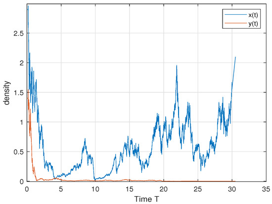
In order to verify Theorem 2, we choose $a=4,b=2,q=5,m=2,c=5,\delta =0.1,$ $h=9,l=1$; then, we have $4-\frac{{0.6}^2}{2}+{\int }_{\mathsf{\Gamma }}[ln(1+0.06)-0.06]\approx 3.81>0$ and $0.1-\frac{{0.6}^2}{2}+{\int }_{\mathsf{\Gamma }}[ln(1+0.06)-0.06]\approx -0.08<0$. Therefore, by Theorem 2, the predator dies out and the prey persists in the sense of time average. This is consistent with Figure 1.

Figure 1. We select the following parameter values: $a=4,b=2,q=5,m=2,c=5,\delta =0.1,$ $h=9,l=1$. The predator y dies out and the prey x persists in the sense of time average.

In order to verify Theorem 3, we choose $a=0.1,b=3,q=6,m=5,c=10,$ $\delta =5,h=5,l=1$; then, we have $0.1-\frac{{0.6}^2}{2}+{\int }_{\mathsf{\Gamma }}[ln(1+0.06)-0.06]\approx -0.08<0$ and $5-\frac{{0.6}^2}{2}+{\int }_{\mathsf{\Gamma }}[ln(1+0.06)-0.06]\approx 4.81>0$. Therefore, by Theorem 3, the predator persists in the sense of time average and the prey dies out. This is consistent with Figure 2.

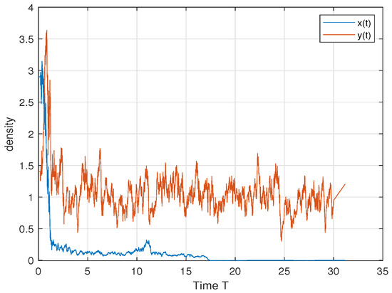
Figure 2. $a=0.1,b=3,q=6,m=5,c=10,\delta =5,h=5,l=1$. The predator y persists in the sense of time average and the prey x dies out.

In order to verify Theorem 4, we choose $a=0.1,b=2,q=5,m=2,c=5,\delta =0.1,$ $h=9,l=1$; then, we have $0.1-\frac{{0.6}^2}{2}+{\int }_{\mathsf{\Gamma }}[ln(1+0.06)-0.06]\approx -0.08<0$ and $0.1-\frac{{0.6}^2}{2}+{\int }_{\mathsf{\Gamma }}[ln(1+0.06)-0.06]\approx -0.08<0$. Therefore, by Theorem 4, both the predator and the prey die out. This is consistent with Figure 3.

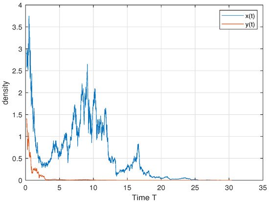
Figure 3. $a=0.1,b=2,q=5,m=2,c=5,\delta =0.1,h=9,l=1$. Then, both the predator y and the prey x die out.

In order to verify Theorem 5, we choose $a=30,b=3,q=6,m=5,c=20,\delta =5,$ $h=5,l=1$; then, we have $5-\frac{{0.6}^2}{2}+{\int }_{\mathsf{\Gamma }}[ln(1+0.06)-0.06]\approx 4.81>0$, $6^2-4(20-6\times 1)=-20<0$ and $5(30-\frac{{0.6}^2}{2}+{\int }_{\mathsf{\Gamma }}[ln(1+0.06)-0.06])-(5-\frac{{0.6}^2}{2}+{\int }_{\mathsf{\Gamma }}[ln(1+0.06)-0.06])\approx 144.24>0$. Therefore, by Theorem 5, both the predator and the prey persist in the sense of time average. This is consistent with Figure 4. In order to further explore the influence of cooperative hunting and group defense on existence, we only change q and c in the above parameters. Only changing q = 6 to q = 15 makes the cooperative hunting intensity increase and does not meet the theorem conditions; Figure 5 shows that the prey perishes. Only changing c = 30 to c = 50 reduces the population defense strength and does not satisfy the theorem condition; Figure 6 shows that the prey perishes. This tells us that when the intensity of cooperative hunting is too large, or the intensity of group defense is too low, it will lead to the demise of the prey, which is also in line with our common sense.

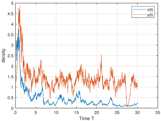
Figure 4. We select the following parameter values: $a=30,b=3,q=6,m=5,c=50,\delta =5,$ $h=5,l=1$. Then, both the predator y and the prey x persist in the sense of time average.

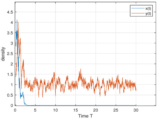
Figure 5. $a=30,b=3,q=6,m=5,c=20,\delta =5,h=5,l=1$. When letting c decrease so that the group defense becomes larger, the predator perishes.

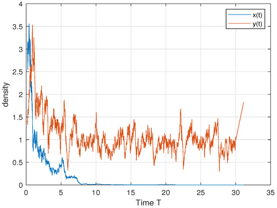
Figure 6. $a=30,b=3,q=15,m=5,c=50,\delta =5,h=5,l=1$. Increasing q makes the cooperative hunting intensity increase, and the prey perishes.

To verify the condition that System (2) without Lévy jump has an ergodic stationary distribution, we assume that $(x_0,y_0)=(0.31,1.725)$, and we choose the following parameter values: ${\sigma }_1={\sigma }_2=0.1,a=2,b=0.7,q=0.6,m=0.12,c=0.1,\delta =2.5,h=0.75,l=0.21$. Then, we have $\delta -\frac{(\phi +1){\sigma }_2^2}{2}>2.5-0.01>0$ and $a+\delta -\frac{1}{2}{\sigma }_1^2-\frac{1}{2}{\sigma }_2^2=0.31+1.725-0.01\ne 0$. As shown in Figure 7, the sample paths are concentrated in the elliptical region, indicating that the system is stochastically stable.

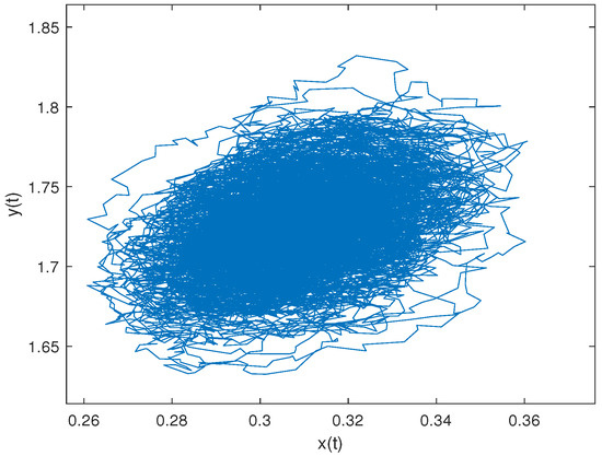
Figure 7. ${\sigma }_1={\sigma }_2=0.1,a=2,b=0.7,q=0.6,m=0.12,c=0.1,\delta =2.5,h=0.75,l=0.21$. The distribution of the sample path in the phase space.

6. Conclusions

This paper discusses the dynamic properties of a predator–prey model with cooperative hunting, group defense, and Lévy noise. First, we prove the uniqueness of the global positive solution of System (2) by constructing a suitable equation. Then, we obtain the theorem that the intensity of white noise and Lévy noise more than a certain extent may lead to the extinction of the population; when the intensity of white noise and Lévy noise is small, if the intensity of cooperative hunting and group defense satisfies an inequality, the two populations can continue to coexist. Furthermore, if the intensity of cooperative hunting is too large or the intensity of group defense is too small, the prey will become extinct. Finally, we conclude that the system has a stationary distribution when there is no Lévy noise.

References

- Leslie, P. Some further notes on the use of matrices in population mathematic. Biometrica 1948, 35, 213–245. [Google Scholar] [CrossRef]
- Leslie, P.; Gower, J.C. The properties of a stochastic model for the predator-prey type of interaction between two species. Biometrika 1960, 47, 219–234. [Google Scholar] [CrossRef]
- Aziz-Alaoui, M.; Okiye, M. Boundedness and global stability for a predator-prey model with modified Leslie-Gower and Holling-type II schemes. Appl. Math. Lett. 2003, 16, 1069–1075. [Google Scholar] [CrossRef]
- Ble, G.; Castellanos, V. Stable limit cycles in an intraguild predation model with general functional responses. Math. Methods Appl. Sci. 2021, 45, 2219–2233. [Google Scholar] [CrossRef]
- Islam, Y.; Shah, F. Functional Response of Harmonia axyridis to the Larvae of Spodoptera litura: The Combined Effect of Temperatures and Prey Instars. Front. Plant Sci. 2022, 13, 849574. [Google Scholar] [CrossRef]
- Ble, G.; Guzman-Arellano, C. Coexistence in a four-species food web model with general functional responses. Chaos Solitons Fractals 2021, 153, 111555. [Google Scholar] [CrossRef]
- Fu, C.; Xu, T.; Wen, S.; Zhang, S.; Liu, F.; Du, C.H.; Zhang, L. Predation Behaviors and Functional Responses of Picromerus lewisi to the Larvae of Ostrinia furnacalis. Chin. J. Biol. Control 2022, 37, 956–962. [Google Scholar]
- Nisal, A.; Diwekar, U.; Hanumante, N.; Shastri, Y.; Cabezas, H. Integrated model for food-energy-water (FEW) nexus to study global sustainability: The main generalized global sustainability model (GGSM). PLoS ONE 2022, 17, e0267403. [Google Scholar] [CrossRef]
- Ali, I.; Rasool, G.; Alrashed, S. Numerical simulations of reaction–diffusion equations modeling prey–predator interaction with delay. Int. J. Biomath. 2018, 11, 1850054. [Google Scholar] [CrossRef]
- Scheel, D.; Packer, C. Group hunting behaviour of lions: A search for cooperation. Anim. Behav. 1991, 41, 697–709. [Google Scholar] [CrossRef]
- Heinsohn, R.; Packer, C. Complex cooperative strategies in group-territorial African lions. Science 1995, 269, 1260–1262. [Google Scholar] [CrossRef]
- Schmidt, P.; Mech, L. Wolf pack size and food acquisition. Am. Nat. 1997, 269, 513–517. [Google Scholar] [CrossRef]
- Bowman, R. Apparent cooperative hunting in Florida Scrub-Jays. Wilson Bull. 2003, 115, 197–199. [Google Scholar] [CrossRef]
- Hannah, K.C. An apparent case of cooperative hunting in immature Northern Shrikes. Wilson Bull. 2005, 117, 407–409. [Google Scholar] [CrossRef]
- Chow, Y.; Jang, S. Cooperative hunting in a discrete predator-prey system. J. Biol. Dyn. 2019, 13, 247–264. [Google Scholar] [CrossRef]
- Andrews, J. A mathematical model for the continuous culture of microorganisms utilizing inhibitory substrates. Biotechnol. Bioeng. 1968, 10, 707–723. [Google Scholar] [CrossRef]
- Sokol, W.; Howell, J. Kinetics of phenol oxidation by washed cells. Biotechnol. Bioeng. 1980, 23, 2039–2049. [Google Scholar] [CrossRef]
- Shen, C. Permanence and global attractivity of the food-chain system with Holling IV type functional response. Appl. Math. Comput. 2007, 194, 179–185. [Google Scholar] [CrossRef]
- Bai, D.; Tang, J. Global Dynamics of a Predator–Prey System with Cooperative Hunting. Appl. Sci. 2023, 13, 8178. [Google Scholar] [CrossRef]
- Du, Y.; Niu, B.; Wei, J. A predator-prey model with cooperative hunting in the predator and group defense in the prey. Am. Inst. Math. Sci. 2022, 27, 5845–5881. [Google Scholar] [CrossRef]
- Yao, W.; Li, X. Complicate bifurcation behaviors of a discrete predator–prey model with group defense and nonlinear harvesting in prey. Appl. Anal. 2022, 102, 2567–2582. [Google Scholar] [CrossRef]
- Fu, S.; Zhang, H. Effect of hunting cooperation on the dynamic behavior for a diffusive Holling type II predator-prey model. Commun. Nonlinear Sci. Numer. Simul. 2021, 99, 105807. [Google Scholar] [CrossRef]
- Pal, S.; Pal, N.; Samanta, S. Chattopadhyay, J. Fear effect in prey and hunting cooperation among predators in a Leslie-Gower model. Ecol. Complex. 2019, 16, 5146–5179. [Google Scholar]
- Qi, H.; Meng, X.; Hayat, T.; Hobiny, A. Stationary distribution of a stochastic predator-prey model with hunting cooperation. Appl. Math. Lett. 2022, 124, 107662. [Google Scholar] [CrossRef]
- Liu, M.; Du, C.; Deng, M. Persistence and extinction of a modified Leslie–Gower Holling-type II stochastic predator–prey model with impulsive toxicant input in polluted environments. Nonlinear Anal. Hybrid Syst. 2018, 27, 177–190. [Google Scholar] [CrossRef]
- Lin, Y.; Jiang, D. Long-time behavior of a stochastic predator-prey model with modified Leslie-Gower and Holling-type II schemes. J. Math. 2016, 9, 121–138. [Google Scholar] [CrossRef]
- Yu, M.; Lo, W. Dynamics of microorganism cultivation with delay and stochastic perturbation. Nonlinear Dyn. 2020, 101, 501–519. [Google Scholar]
- Higham, D. An algorithmic introduction to numerical simulation of stochastic differential equations. SIAM Rev. 2001, 433, 525–546. [Google Scholar] [CrossRef]
- Slimani, S.; de Fitte, P. Dynamics of a prey-predator system with modified Leslie-Gower and holling type II schemes incorporating a prey refuge. Discret. Contin. Dyn. Syst.-Ser. B 2019, 24, 5003–5039. [Google Scholar]
- Han, B.; Jiang, D. Stationary distribution, extinction and density function of a stochastic prey-predator system with general anti-predator behavior and fear effect. Chaos Solitons Fractals 2022, 162, 112458. [Google Scholar] [CrossRef]
- Qiao, M.; Yuan, S. Analysis of a stochastic predator-prey model with prey subject to disease and Lévy noise. Stochastics Dyn. 2019, 19, 1950038. [Google Scholar] [CrossRef]
- He, X.; Liu, M.; Xu, X. Analysis of stochastic disease including predator-prey model with fear factor and Lévy jump. Math. Biosci. Eng. 2023, 20, 1750–1773. [Google Scholar] [CrossRef] [PubMed]
- Lipster, R. A strong law of large numbers for local martingales. Stochastics 1980, 3, 217–228. [Google Scholar]
- Khasminskii, R.; Klebaner, F. Long term behavior of solutions of the Lotka-Volterra system under small random perturbations. Ann. Appl. Probab. 2001, 11, 952–963. [Google Scholar] [CrossRef]
- Khasminskii, R. Stochastic Stability of Differential Equations. In Stochastic Modeling and Applied Probability; Springer: Berlin/Heidelberg, Germany, 2012; pp. 99–136. [Google Scholar]
Disclaimer/Publisher’s Note: The statements, opinions and data contained in all publications are solely those of the individual author(s) and contributor(s) and not of MDPI and/or the editor(s). MDPI and/or the editor(s) disclaim responsibility for any injury to people or property resulting from any ideas, methods, instructions or products referred to in the content. |
© 2023 by the authors. Licensee MDPI, Basel, Switzerland. This article is an open access article distributed under the terms and conditions of the Creative Commons Attribution (CC BY) license (https://creativecommons.org/licenses/by/4.0/).