Appendix A. The Space of Bicircular Quartics
Here, we give further details regarding the stratification defined by the elliptic discriminant , and prove Proposition 2.
First, for
K as in Equation (
3), we read off the tangents to
K at
I from the lowest-order terms in the affine view
:
Unless
or
,
I is indeed a node, with distinct tangents
Here,
are the two
singular foci of
K. These are usually not foci (as noted in
Section 2); exceptions will be discussed shortly. For future reference, we observe that
are the roots of
, the leading coefficient of
(Equation (
4))—so
has at most one root.
In particular, when
,
K has nodes at
I and
J. In fact, there are no other singularities. It is useful to verify this directly by showing that the system
has no solution with
. We scale coefficients so that
:
For these all to vanish, either: ; ; ; or . In each case, a factor of vanishes. To conclude, K is an elliptic curve.
Conversely, by considering the factors of , we find that implies that K is non-elliptic. In particular, the 2-dimensional strata —defined by exactly one distinct factor of vanishing—consist of rational or reducible curves satisfying one of the following descriptions (here, we normalize by , except when ):
Trinodal: : nodes .
Conics: .
Concentric circles: , center O.
Circle pairs: .
Circle pairs: .
For the last two, the “centers” (singular foci) represent points on either the x-axis or the y-axis as symmetry requires. Of the five non-elliptic cases, we refer to the last three as circular, and to the first two as rational-non-circular.
Curves in the 1 and 0-strata (two or three factors vanish) play a special role. In case
,
correspond to the four
mirrors of reflection symmetry (
Appendix E); in case
,
are the four mirrors (however, the first two require the imaginary coefficients
).
Before turning to the proof of Proposition A1, we make a few additional observations. First, a curve K which is a product of circles/lines has no foci. Second, is never a focus of any ( consists of the “two points at J”, when J is a node, and the two ideal points of a conic otherwise). A finite node never gives a focus ; in particular, in the trinodal case is not a focus. In fact, is never a focus of any . The remaining issues addressed in the proof of the following result have mostly to do with singular foci and Cassinians.
Proposition A1. Let k be a quartic in rectilinear position (Equation (4)), with focal discriminant (Equation (5)) and elliptic discriminant (Equation (6)): (a) is a focus of k if and only if it is a simple root of ;
(b) k is an elliptic curve ;
(c) k is a rational non-circular ;
(d) k is circular or degenerate .
Proof. We already noted the first equivalence in (b). The second follows from Equation (
1), and likewise for (c) and (d). For (a), there are two possibilities to consider:
, and
.
Case First, assume is a focus. Then, ; otherwise, has a simple root , so cannot be a branch point of . Thus, k is in fact quadratic in v. Since k cannot have two distinct roots, it must have a double root, so .
To see that
must be a
simple root of
, we consider the different possibilities for
K. All roots are simple in the elliptic case
. Likewise, in the conic case
, both roots are simple (see Equation (
5)). For the trinodal case
, the only non-simple root is
(again, see Equation (
5)), but
. Finally, the circular cases have no foci so need not be considered.
Conversely, let be a simple root of . Then, has a double root . Consider the corresponding finite point . We know that cannot be the node of a trinodal curve, which yields a double root of . It cannot be a double point for one of the circular cases; in these cases, is a “square” (e.g., when , ). The only possibility is that is a regular point of K, but a ramification point of isotropic projection —that is, a point of isotropic tangency. So is a focus.
Case We already dealt with (which only arises in cases or ), so we need only consider the case . When , this is just the case of a rectangular hyperbola, and there is nothing new to consider.
When , K is a Bernoulli lemniscate. In this case, has simple roots . Note that , i.e., is a singular focus. In fact, , , and is a non-zero constant. (Geometrically, the isotropic line meets Kfour times at I, a biflecnode, and is a triple focus.) Thus, is a branch point of , that is, a focus of K.
Finally, when and , K is a Cassinian. In this case, there are two triple foci and two ordinary foci—all of which are foci and simple roots of . The two types of foci correspond to the following two subcases: (i) , which gives rise to the singular foci (as for the lemniscate); (ii) , which gives the ordinary foci satisfying , i.e., . □
Appendix B. Concyclic Confocal Families
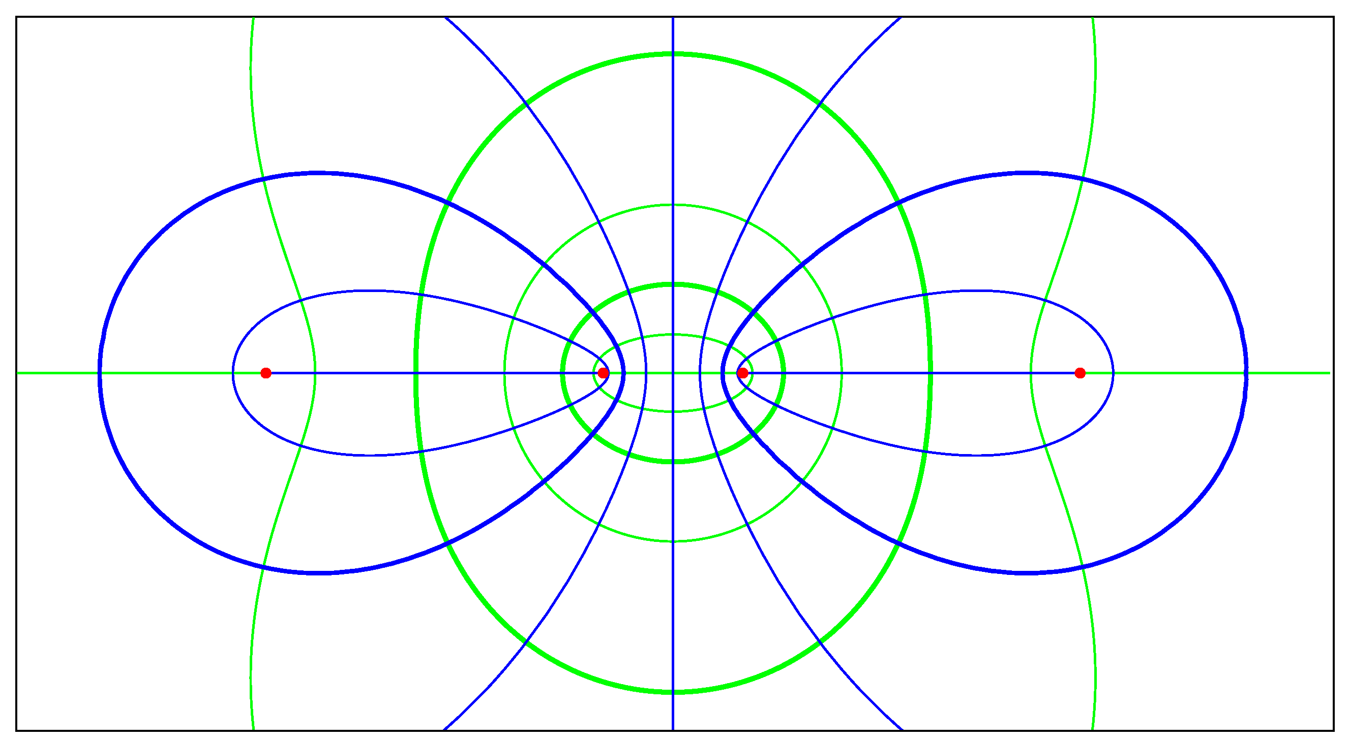
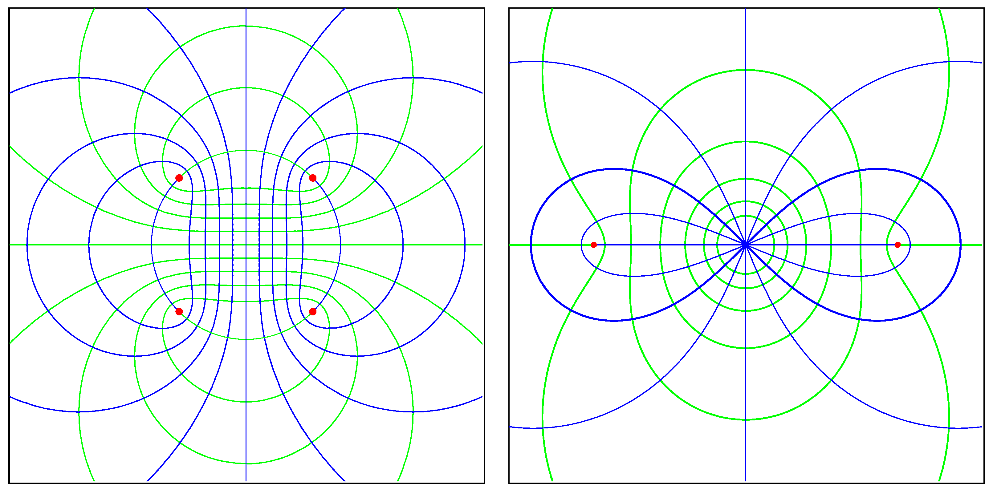
Figure A1 shows the orthogonal pair of foliations
in case
(for the particular choice
). The mirrors are the
x and
y axes and the
real/imaginary circles
(
Appendix E). Each quartic is two-circuited; in one foliation (blue), the two circuits of a curve are swapped by reflection in the
y-axis; in the other foliation (green), the two circuits are swapped by inversion in
.
Figure A1.
Confocal family of type (); the foci are the four red points. Each irreducible quartic in is two-circuited—e.g., see bold blue/green curves (the bold blue one is the unique Cassinian in ).
Figure A1.
Confocal family of type (); the foci are the four red points. Each irreducible quartic in is two-circuited—e.g., see bold blue/green curves (the bold blue one is the unique Cassinian in ).
In this example, all foci are on the
x-axis. But this is not the only possibility for a confocal family with
. To determine all subcases, consider the normalized focal discriminant
(Equation (
8)) and corresponding “normalized” elliptic discriminant:
The curve k is elliptic unless , i.e., or .
Thus, in the present case
,
k is elliptic for
; that is, unless
k belongs to one of the circular cases
or
In fact, the circular locus
(where
or
∞) divides the
-plane into the following three reduced elliptic strata
indicated in
Figure A2:
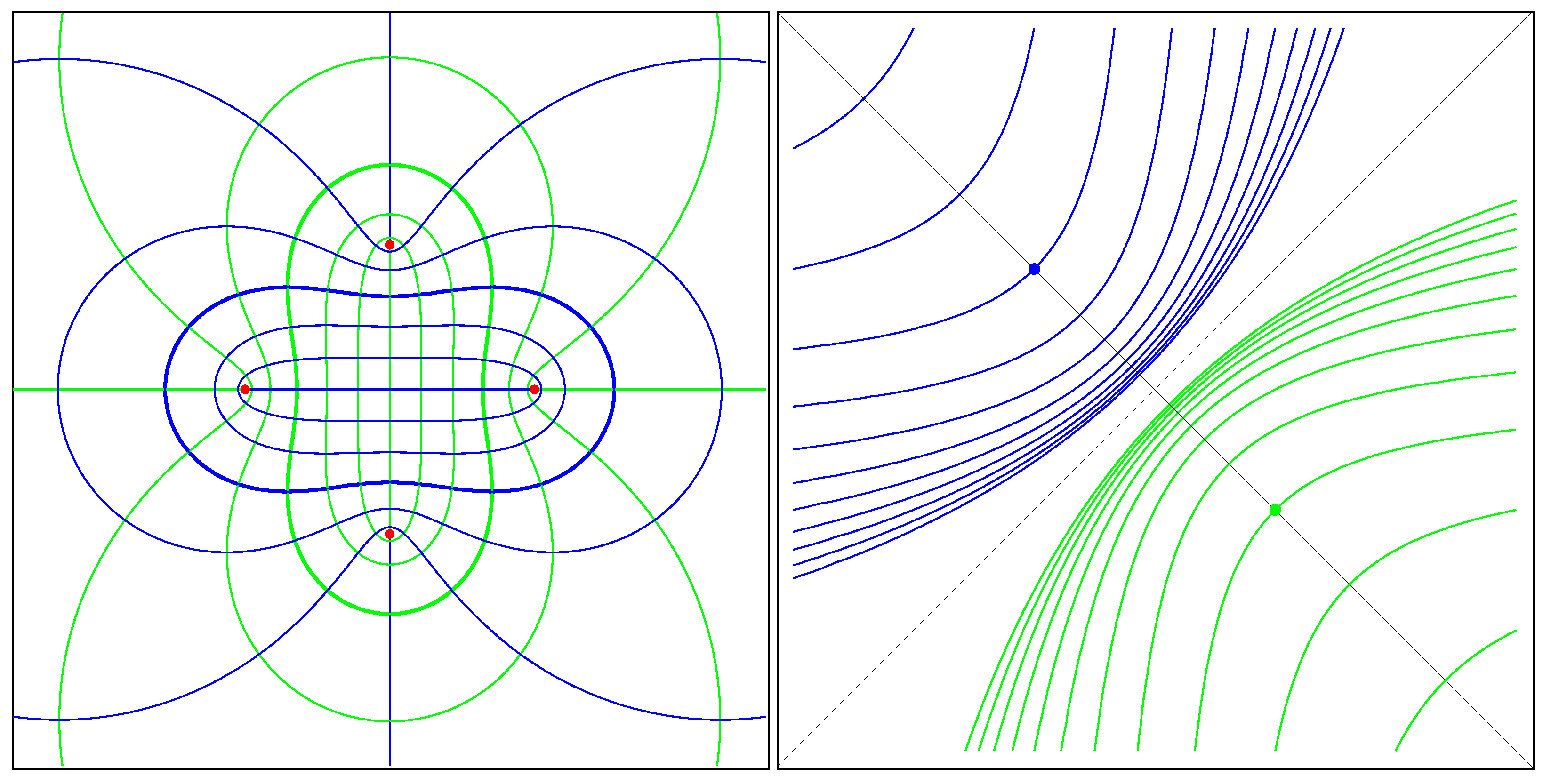
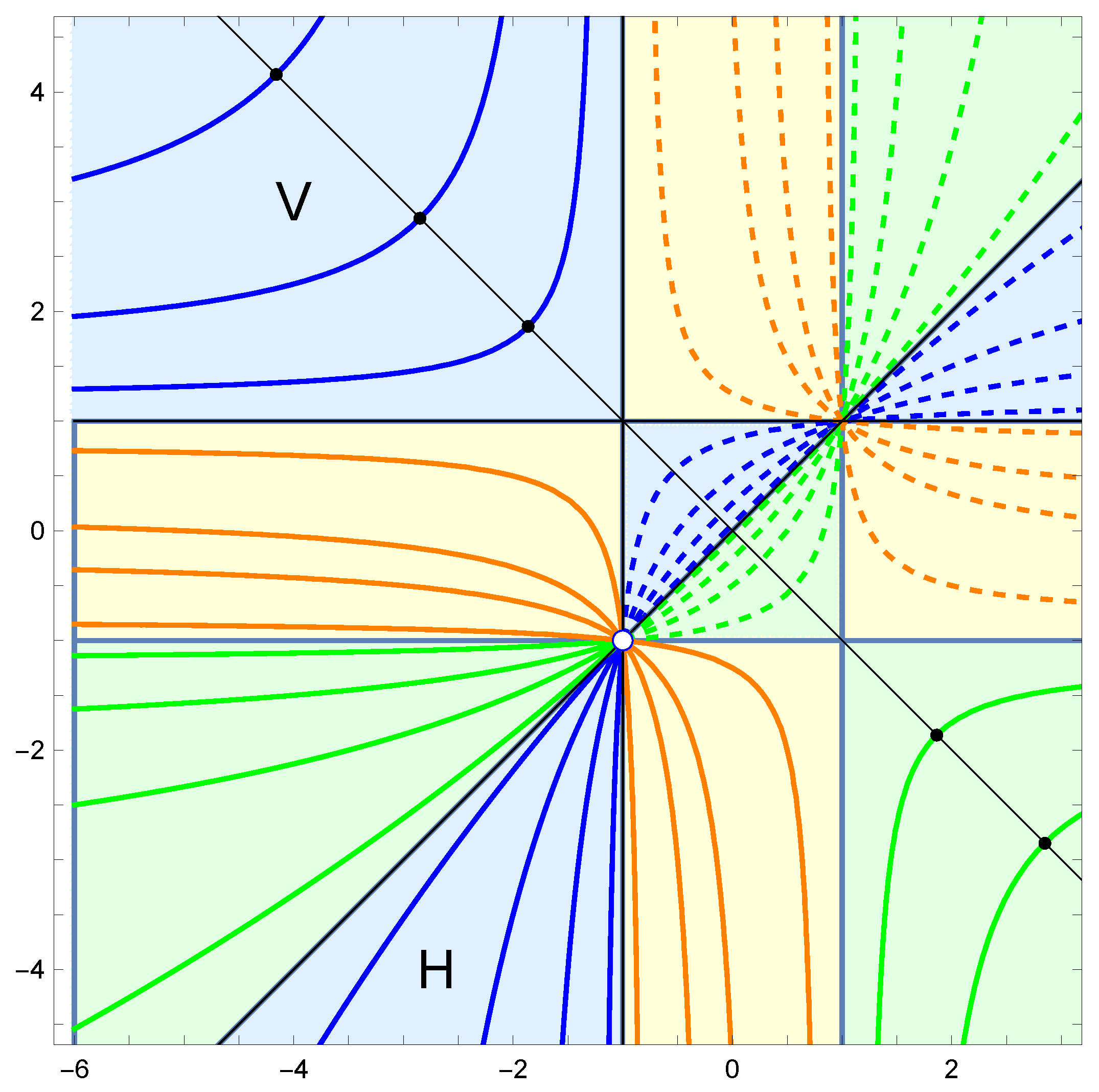
Figure A2.
The -plane is foliated by hyperbolas: represents a confocal family with concyclic foci on the x-axis (blue), y-axis (green), or unit circle (orange). H/V denote (blue) regions whose points represent horizontal/vertical trajectories. Dashed curves are explained in Remark A2.
Figure A2.
The -plane is foliated by hyperbolas: represents a confocal family with concyclic foci on the x-axis (blue), y-axis (green), or unit circle (orange). H/V denote (blue) regions whose points represent horizontal/vertical trajectories. Dashed curves are explained in Remark A2.
We note that the three cases correspond to the four roots
of
being
real (
),
imaginary (
), or of
unit modulus (
)—see
Figure A3, left. In particular, the foci are always concyclic; in fact, the three subcases are all inversively equivalent.
Remark A1. We expand on the last comment. The two subcases and are related by -rotation of the -plane. The subcase is related to the first via the Cayley map (or the corresponding transformation on the -plane). We note that is an order three map which cyclically permutes the real mirrors in case .
Although this relationship implies that there is no essential difference from the other subcases, our descriptions have to be modified somewhat. For instance, note that the anti-diagonal does not intersect any of the corresponding hyperbolas—shown in orange in Figure A2. In other words, there are no Cassinians in such -concyclic confocal families. There are, however, curves which play essentially the same role. These curves—which are represented by points along the line (i.e., )—are obtained from Cassinians via the Cayley map, so we call these curves Cayley Cassinians.
Figure A3.
(Left): The confocal family ; green/blue curves are horizontal/vertical trajectories of . (Right): Confocal family of type . The blue curves are Booth lemniscates; the bold one is the Bernoulli lemniscate (the unique Cassinian in the family). Green curves are -inverted ellipses.
Figure A3.
(Left): The confocal family ; green/blue curves are horizontal/vertical trajectories of . (Right): Confocal family of type . The blue curves are Booth lemniscates; the bold one is the Bernoulli lemniscate (the unique Cassinian in the family). Green curves are -inverted ellipses.
Returning to the subcase
, the anti-diagonal meets both branches of each hyperbola
—yet only one Cassinian appears in
Figure A1. The apparent contradiction is resolved by the following remark, which explains one of the main differences between the two cases
, and between confocal vs. orthogonal families.
Remark A2. Though a confocal family is understood here to consist of real curves, a given curve in the family may have an empty real locus in case . Note that when . In all other cases, f has a minimum either or . Thus, f has no real points whenever . In Figure A2, solid portions of hyperbolas indicate curves in the foliation on . In the blue region (where ), every point on an upper branch represents a curve in the orthogonal family (in fact, a vertical trajectory of ). On the other hand, the dashed portions of certain hyperbola branches indicate “empty” curves, e.g., on the lower branch of a hyperbola in the blue region (where ), only the points up to (indicated by a white dot) represent (horizontal) trajectories in the foliation . Finally, ◯ itself represents the “squared circle” in , which has no foci, and does not belong to the confocal family , as strictly defined. But as Figure A1 illustrates, the unit circle (like all real mirrors) clearly belongs to the orthogonal family . For convenient reference, we list the types of confocal families (and their figures):
(
Figure A1;
Figure A3, left)) The four roots
of
are always concyclic. In each subcase
,
K is an elliptic curve forming two smooth closed curves in
. In fact, the three subcases are inversively equivalent.
(
Figure 2) For
,
takes all real values. The four roots
of
are
rhombic (non-concyclic, except when
, i.e.,
). The bicircular quartic
k is an elliptic curve whose real locus consists of one smooth closed curve in
.
(
Figure A3, right)
k is a trinodal quartic with a (real or imaginary) pair of foci
. If
, the double point at the origin is a node and
k is a
Booth lemniscate. When
, it is an acnode, and the rest of
k appears as an
oval in
. The case
may be regarded as the transitional case between
and
.
k is a conic () with a (real or imaginary) pair of foci; the ellipses () and hyperbolas () are related to the curves of type by inversion in the unit circle.
Appendix C. Remarks on the Classical Notion of Focus
Aside from providing geometrical intuition, our foray into the classical heuristics of foci is meant to point out how confusions arise, and how they are resolved by Definition 1.
Focal properties of conics have been known since antiquity, but it was Kepler who introduced the Latin word
focus. Poncelet interpreted a conic’s foci as points of intersection of the isotropic tangent lines through
I with those through
J. Plücker then used the latter to
define (real and complex) foci for curves of higher degree (see [
16], p.160).
Here, we are mostly concerned with real foci (-foci), a term which distinguishes such real points from the general -foci of Plücker’s definition, and from the foci of Definition 1.
In the case of an ellipse or hyperbola, we note that there are two isotropic tangents from each point . The tangents from I are paired with those from J via complex conjugation (as is the case for any real curve); consequently, two of the four -foci are real foci.
More generally, the number m of tangent lines to a curve F from a general point P is the class of F—which can be shown to be independent of P, and is in fact the degree of the dual curve . For a curve with nodes and cusps (and no more complicated singularities), one of Plücker’s equations is .
Letting , one accordingly expects -foci and m -foci. Indeed, this is usually the case for non-circular curves. Thus, for example, an ellipse or hyperbola, which has class , has two real foci. (A parabola would appear to be an exception, but according to Definition 1, it has a second focus at .)
Now consider a circle that has a regular point at I. If P is a nearby point, there are two tangents from P since . If P is allowed to approach I, these will merge into one tangent at I (which may be viewed as contributing two to the class m). This would presumably explain why the circle has just one real focus, namely, its center.
But a circle’s center is a singular focus—the classical term for a focus resulting from a tangent at I—often viewed as quite different from an ordinary (or simple) real focus. (According to Definition 1, a circle has no foci; on the unit circle , e.g., is evidently 1-1.)
Next, consider a bicircular quartic with a pair of nodes at the circular points. With , , Plücker’s equation gives . Of course, such curves do not have so many real foci. In fact, there can only be six distinct tangents through I, given that each of the two tangents at the node I counts (at least) twice. Thus, if we discard the resulting pair of singular foci, we would generally expect to obtain four real foci, as in Proposition 1.
But simply
discarding the singular foci is not quite correct. This can be seen by considering the special bicircular quartics known as
Cassinians (or
ovals of Cassini, after the astronomer who proposed such curves as candidates for planetary orbits [
1]). Cassinians belong again to the binodal case (
or 3), but happen to be
biflecnodal [
18,
34]; that is, each of the two tangents at
I meets its branch
three times. Such a tangent also meets the other branch once, thus accounting for all
four intersections of the tangent with the curve. Whereas the tangent to a circle at
I results in a
double focus (classical term), the two singular foci of Cassinians are
triple foci. Further, in view of the fact that a Cassinian has class
, such a curve accordingly has only two ordinary real foci. (A similar anomaly arises for
Cartesians, which are bicircular quartics with
; these have triple foci by virtue of their cusps at
I, along with three ordinary foci.)
Yet Cassinians are plainly seen to occur in confocal families of bicircular quartics sharing four foci. Thus, in contrast with Proposition 1, the classical enumeration of foci would appear to be full of caveats: A bicircular quartic K has four foci, provided the two singular foci are discarded—except when K is a Cassinian (or Cartesian), in which case the singular foci should not be discarded!
In other words, triple foci count, even though double foci do not. But from the standpoint of Definition 1, this is easily explained: What ties the triple and ordinary foci of Cassinians together—and sets both apart from the double foci—is that they are branch points of isotropic projection. (In fact, they are both simple branch points.) Likewise, quadruple foci, etc., are foci (though such higher order branch points of do not occur in our examples).
Appendix D. Siebeck’s (Other) Theorem
Note that the identity of Siebeck appears to be a bit uncertain. He is likely the author of the Ph.D. thesis listed as F. H. Siebeck, Universität Breslau 1845, “On conic surfaces for any circumscribed surface”. In the important reference [
35], the author of [
36] is listed as J. Siebeck—mistakenly, we believe. Regardless, Siebeck seems to be mostly known for
Siebeck’s theorem [
36], which characterizes the zeros of
as the foci of a related conic (see [
37] for the hyperbolic case). But his result on quartics and elliptic functions also deserves to be well known—hence, this brief appendix on his paper [
3].
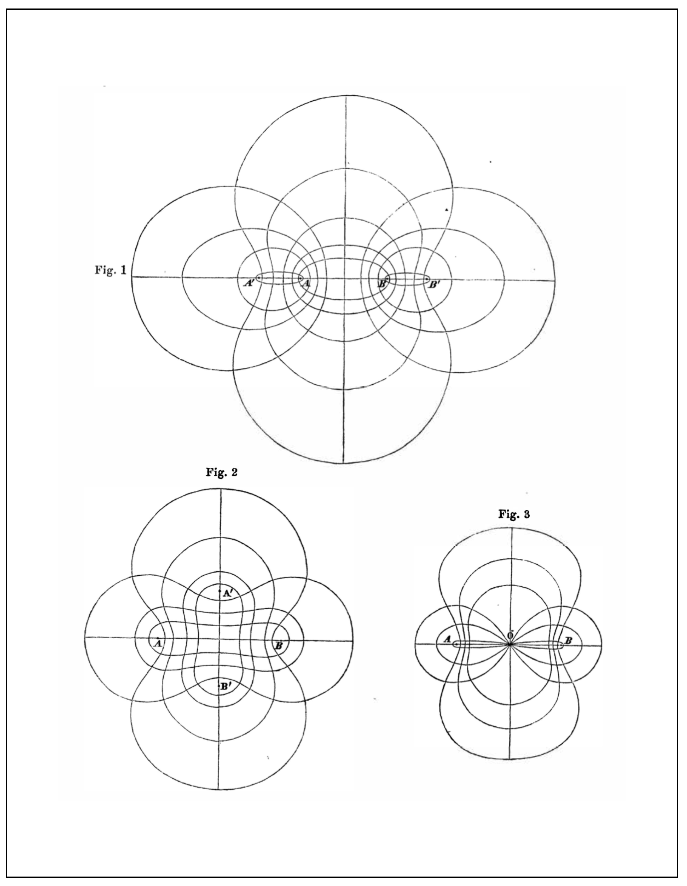
Figure 1 itself delivers on the promise of an earlier paper [
38], “On the graphical representation of imaginary functions”. For this reason, and because of the satisfying parallel to
and confocal conics, it is the kind of thing one might expect to see browsing textbooks “at random”. But so far, we have found just [
39], which shows Siebeck’s first graphic.
In fact, it is hard to tell from the literature how much attention Siebeck’s paper received at the time. What does seem clear is that Siebeck’s work should not be viewed as an isolated contribution, and the general theme (B) would have seemed much more mainstream over one hundred years ago than it is today.
Darboux studied the confocal systems of Cartesians and
cycliques (or bicircular quartics) [
28,
40,
41,
42,
43,
44], in the context of the theory of projective algebraic plane curves, triply orthogonal systems of surfaces and spherical conics. (Note: though the connection between bicircular quartics and spherical conics was made in Siebeck’s time, the intrinsic hyperbolic setting for conics seems to have received much less attention—see, however, [
4,
45,
46,
47].) Darboux and others investigating such topics were building on the geometric contributions of Poncelet, Plücker [
17], Chasles [
48], and Kummer [
49], to name a few. Over several decades, a number of authors [
27,
50,
51,
52,
53,
54,
55,
56,
57] also explored the intimate connections between such curves and parallel developments in complex function theory—the Jacobi and Weierstrass elliptic functions, their double periodicity and addition theorems. (See [
58] for historical background and many additional references.)
Returning to the Siebeck paper itself, we note that direct verifications of the curve parameterizations (along the lines discussed in
Section 1) involve elliptic function identities; the computations are much more complicated than in the case of Euclidean conics. In the course of developing a manageable approach to such computations, it seems that Siebeck also discovered several of the main properties of such curves. He did so prior to the closely related work of other authors—e.g., Darboux (on
cycliques) and Casey (on
bicircular quartics)—and without the benefit of somewhat more systematic treatments of foci, including his own [
36].
Although Plücker’s general notion of foci was well established by 1860, Siebeck’s provisional treatment of foci for the curves in question probably reflected the state of understanding at the time. Siebeck considers three different features of his confocal families to establish the connection with accepted notions of foci in projective geometry. Namely, he finds analogues of the string and reflection properties of conics, and also the orthogonal pair of foliations with singularities at the presumed foci.
Although the first paper [
38] suggests that Siebeck’s starting point was the parameterization by elliptic functions
and
, he begins [
3] with an analogue of the string property to define the class of curves as follows. Fix a pair of points
, and let a general point
P on a curve satisfy an equation of the form
where
and
denote the sum and difference of distances from
P to
A and
B, and
m and
n are real numbers.
By purely algebraic means, Siebeck discovers the underlying geometric symmetries of Equation (
A2) to show that there are actually
eight special points with respect to which similar equations for the same curves may be written down. (Thus, he locates half of the
sixteen complex foci of his curve families.) He then determines that exactly
four of the latter points are real, and finds two qualitatively distinct
types of such curve families, depending on the pattern of the quadruple of points. Ultimately, the two cases turn out to correspond to the ramification points of the elliptic functions
and
.
Figure 1 illustrates the main qualitative difference between the orthogonal systems parameterized by
and
. In the case of
(upper curves in the figure), the four foci
are
concyclic (in fact, collinear). For the elliptic cosine
(shown on the lower left), the foci are
non-concyclic (and lie symmetrically on an orthogonal pair of axes). Finally, there is an intermediate case (lower right), in which the elliptic function becomes elementary as a pair of foci in either of the previous two cases collide.
Next, Siebeck shows that the family of curves breaks up into two orthogonal subfamilies, concluding: “The points are therefore foci in the usual sense”. He does not elaborate on “the usual sense”, but it seems likely that he was familiar with Kummer’s theorem.
The striking heuristic argument of Kummer, based on Plücker’s definition of foci, goes as follows. Assume a family of curves
such that exactly two such curves
meet orthogonally at a given general point
. The latter condition seems evident in
Figure 1, and is exactly what Siebeck verifies algebraically (seemingly for real planar points
). The orthogonality condition may be written
. Kummer apparently assumes analytic dependence on
a, so the latter equation holds also at complex points—which must therefore include the “invisible" points of intersection of arbitrarily nearby curves in the planar foliations by
. Therefore, in the limit where a pair of such curves coincide,
and the earlier equation becomes
. This may be thought of as the condition of “self-orthogonality” of the vector
with respect to the complex-linear extension of the Euclidean metric on the plane. In other words,
is an
isotropic (or
null) vector, i.e., it has an
imaginary slope . This occurs because the family
has an
envelope belonging to a set of isotropic lines. These are in fact isotropic tangents to each curve in the family
, which is therefore confocal.
The third focal property which Siebeck establishes for
is a generalization of the focal property of conics. Given a point
P on one of the curves
, let
be its angular coordinate, and let
be the angular coordinates formed by the vectors from each of the four foci to
P. Examining each of the two types of systems
, Siebeck verifies that in both cases, the following relationship holds among the five angles:
In other words, up to the addition of , the equation holds. Further, Siebeck argues, as two of the four foci tend to infinity, that f tends to a conic, and the latter equation becomes —which is a way of expressing the familiar reflection property of the ellipse.
We remark that the analogy to the classical reflection property becomes much closer when Siebeck’s quartic curves are interpreted as non-Euclidean conics [
4,
59]. We note also that Equation (
A3) can be immediately read off from the quadratic differential
defining the family of curves as trajectories (
Section 5).
Appendix E. Circles of Inversion for Circular Cubics
In this appendix, we prove Theorem 1 on the existence of four orthogonal mirrors. A mirror
C is given by an equation:
For
, we may consider the center
c and squared radius
,
If the coefficients are real, then C may be real (real center and real radius), or imaginary (real center and imaginary radius). Otherwise, C is complex, in which case there is a complex conjugate mirror . Point circles are excluded.
For a mirror with a center at the origin and squared radius , inversion is given by —essentially, the quadratic transformation in . For , inversion is obtained by conjugating such by translation. The meaning of orthogonal for non-real mirrors is discussed below.
We first show that a bicircular quartic can be put in rectilinear position; for this, it suffices to find an orthogonal pair of real circles of inversion since these become perpendicular axes after inversion about one of the two finite points of intersection. Further, since the inverse of a bicircular quartic with respect to a general point on the curve is a circular cubic, the problem reduces to finding such a pair of circles for a given circular cubic. We now describe the elementary construction for this purpose, outlined in [
19]; see
Figure A4.
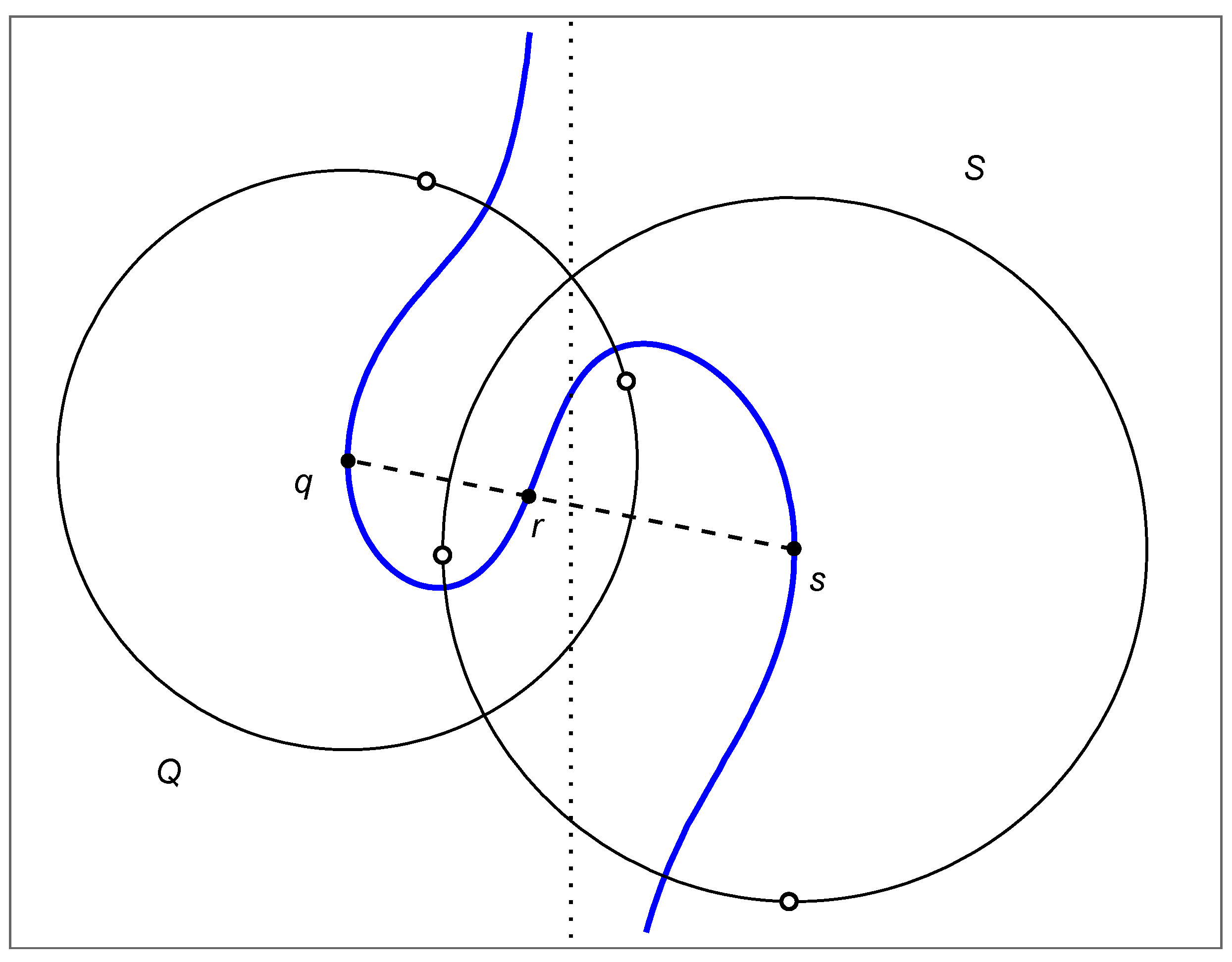
Figure A4.
A one-circuited circular cubic and its two real circles of inversion (centers ); real foci ∘ (two on each circle); asymptote; collinear points .
Figure A4.
A one-circuited circular cubic and its two real circles of inversion (centers ); real foci ∘ (two on each circle); asymptote; collinear points .
Let be a circular cubic, assumed to be real and nonsingular. We may also assume that the unique real ideal point p is not a flex (which will be the case, e.g., if a bicircular quartic is inverted about a generic point). By rotation, we may assume that f has cubic term , so . There are four tangents to f from p (aside from the tangent at p itself), namely, the vertical lines , where is one of the four roots of the discriminant . (f being of class six, four tangents from p, was expected.) When the point of tangency is translated to the origin, the cubic has the form . Then, one easily verifies that f is symmetric with respect to inversion in the circle . Here, the “radius” is non-zero since f is nonsingular. To be precise, f is preserved by the inversion in the sense that (the extra linear components being “superfluous”).
Translating the center of the circle back to the point of tangency of the original curve gives the corresponding mirror . One can do the same for each of the four roots to obtain four mirrors .
We want to find real mirrors; for this, it suffices to show that at least two of the points are real. We recall that all nonsingular real cubics may be divided into two classes: those whose real locus consists of the odd circuit alone, and those which also have an even circuit (a simple closed curve in ). The key is to examine the mirrors with centers on the odd circuit (unbounded real connected component) of f.
Figure A4 shows a cubic of the former type, together with the vertical asymptote
(the tangent line to
f at
p); the argument works just the same for two-circuited cubics.
Since p is not a flex, meets in a finite real point and extends to the left and right of this line. In fact, has a left-most point q and a right-most point s, which are points of vertical tangency. Thus, q and s are real centers of inversion as constructed above. But we still need to verify that the corresponding mirrors have real radii , and that they meet orthogonally.
We denote these two mirrors and . Let be the line joining their centers, and let r be the point on obtained as the third intersection of L with f. (L cannot intersect since it would have to meet it twice.) Viewing as a topological circle containing p, the four points have cyclic order on . Regarding , by restriction, as a homeomorphism of the circle , note that swaps p with q and swaps r with s. Thus, has real fixed points “between” each pair. But the fixed points of belong to Q, which must therefore be real. Likewise, swaps points according to , and S is real.
For heuristics, it is expedient at this point to identify the composition of circle inversions with a Möbius transformation of . In this sense, T must be elliptic—with a pair of real fixed points —otherwise, T would have infinite order. In fact, , so . In other words, inversions and commute, which can only happen if Q and S meet perpendicularly. Thus, a circular cubic has an orthogonal pair of mirrors as required for the rectilinear position.
Some additional remarks may be in order. Suppose C is any mirror of a circular cubic f and ℓ is one of the four isotropic tangents through the circular point I. If K is the finite intersection point of C with ℓ, then inverts to the isotropic line . This line must also be a tangent since takes f to itself. Thus, K is among the sixteen (complex) foci of f, four of which must lie on C. The same argument applies to each mirror; thus, we established the last part of the classical result.
Next, we comment on the remaining mirrors . In the one-circuited case, these are a complex conjugate pair of mirrors determined by the two non-real centers on . In the two-circuited case, the centers of are real, these being the left- and right-most points on ; it turns out that one mirror T is real and the other U is imaginary. Evidently, T is orthogonal to Q and S, and consequently all four mirrors are mutually self-inverse.
When a non-real mirror is involved, the notion of
orthogonality requires a definition. First, let
be real circles, with centers
and squared radius
. If
and
C meet perpendicularly in
, the Pythagorean theorem gives
. Let
C, as in Equation (
A4), be represented by the vector
, and likewise for
. One finds, using Equation (
A5), that perpendicularity is equivalent to orthogonality with respect to the bilinear form
We note the relation to
Möbius circle geometry [
60]. If a plane
and sphere
in
intersect in a circle
A, there corresponds a planar circle/line
C as above via stereographic projection
. It’s coefficients are:
. Then a short computation yields the Minkowski inner product on vectors
representing spherical circles:
. In particular, note that
for real circles, which explains why there can be at most three mutual orthogonal real mirrors.
Proceeding to the general case, orthogonality may be defined by the same equation
by complex bilinear extension. We note some formal consequences of this definition. First, no orthogonal pair can be imaginary. For if
C and
are two such circles, we can assume
, for simplicity, and obtain
This leaves three possibilities for a set of mutually orthogonal mirrors:
(1) Three real mirrors and one imaginary mirror.
(2) Two real mirrors and two complex conjugate mirrors.
(3) Two pairs of two complex conjugate mirrors.
However, the third type cannot exist. Suppose is the vector representation of a complex circle, where v and w are circles with real coefficients. The condition that C be orthogonal to is . Note that this implies one of v and w is a real circle and the other is imaginary.
Now assume there are two pairs of complex mirrors
that are mutually orthogonal. Taking the inner product of
with
, we have
Comparing this with the equation
we conclude that the real and imaginary part of each is orthogonal to both the real and the imaginary part of the other. But either
or
is an imaginary circle, and imaginary circles cannot be orthogonal to each other.
To conclude this section, we list the mirrors and complex foci of bicircular quartics F in standard position. First, the x and y axes are a pair of real mirrors. Further, one easily verifies that the circles are mirrors using with . (All mirrors can also be “derived” from the elliptic discriminant; each is found by setting three factors of equal to zero.) Thus, in case , there is a real circle and an imaginary circle . In case , there is a pair of complex conjugate mirrors with squared radius . The apparent departure from the cubic case is rather striking: the two circular mirrors are “concentric”, with center not on the curve. But there is no contradiction to any of the above general claims about systems of mirrors; circle centers, being double foci, do not respect inversive symmetry.
We list the sixteen complex foci for case
:
Likewise, the sixteen complex foci for
are


