Abstract
This brief discusses the use of quantized control with actuator saturation to achieve the local synchronization of master–slave fractional-order neural networks (FONNs). A refined sector condition (RSC) is proposed that addresses the issue of the simultaneous quantizer effects and actuator constraints. The RSC is used in the theoretical analysis of local synchronization in drive-response systems. The analysis employs inequality techniques on the Mittag–Leffler function and fractional-order Lyapunov theory. Additionally, this paper presents two convex optimization algorithms that aim to minimize the actuator’s costs and expand the admissible initial area (AIA). Finally, this paper employs a three-neuron FONN to demonstrate the efficacy of the proposed methods.
Keywords:
fractional-order neural networks; FONNs; quantized control; actuator saturation; refined sector condition; RSC; local synchronization MSC:
03F03
1. Introduction
Synchronization is a significant dynamic behavior of coupled systems that has garnered considerable attention due to its successful applications in various fields such as information sciences [1], secure communication [2], and combinatorial optimization [3]. In secure communication, chaotic drive and response systems are employed to generate pseudorandom numbers that serve as encryption and decryption keys, respectively. It is important to note that even a minor error between the decryption and encryption keys can result in decryption failure due to the sensitivity of the keys. Recently, there has been growing interest in using fractional calculus to model and analyze various systems, including neural networks. The benefit of fractional calculus lies in its ability to describe the fundamental characteristics and retention of the system model more precisely than conventional integer-order calculus [4,5,6,7,8,9]. One of the main advantages of using fractional-order derivatives is that they possess infinite memory, which is particularly important in neural network models. Conventional integer-order neural networks have constraints in representing the enduring memory of neuron synapses, which is a crucial feature of biological neural networks [10,11,12]. To address this limitation, the development of fractional-order neural networks (FONNs) based on fractional-order differential equations is crucial. This is because the electroconductibility of the plasma membrane exhibits fractional-order properties, and real capacitors have been shown to be “fractional” in practical applications [12,13]. Therefore, adding fractional capacitors to the large-scale integrated circuits of FONNs can improve the efficiency of information manipulation and the precision of the model [10]. As a result, FONNs have received substantial attention, and remarkable outcomes such as synchronization have been achieved [14,15,16,17].
With the growth of information and communication technology, networked control methods, such as event-triggered control [18], sampled-data control [19,20], intermittent control [17,21], and quantized control [15,22,23,24], have become increasingly popular in engineering applications. These methods share the common feature of using digital and isolated control intelligence. In contrast to conventional regulation approaches [14,16,25,26], networked control schemes can decrease control costs and network-introduced loads within a restricted and crowded communication capacity. When implementing extensive FONNs, where factors such as computing power, storage capacity, and communication resources are limited, alleviating these constraints has become a top priority. The quantizer used in quantized controllers can act as an information coder that converts continuous signals into piecewise constant ones, transmitting incomplete data sent to the CPU, thus saving energy and releasing congested I/O ports. However, most relevant results have primarily focused on integer-order systems, as classical Lyapunov techniques and inequality analysis methods cannot be applied to fractional-order systems. Therefore, the primary objective of this brief is to examine the stabilization of FONNs when subjected to quantized control.
It is important to note that all the aforementioned results assume that there are no constraints on the control input [14,15,16,25,26,27,28]. However, in practical applications, actuators often experience saturation owing to the constrained amplification ability of operational amplifiers in the physical configuration, resulting in control input with an amplitude constraint. This saturation phenomenon can degrade system performance or cause the instability of closed-loop systems. The sector condition is commonly used to address the saturation nonlinearity issue [21,29,30,31]. For instance, the problem of analyzing the -gain and exponential synchronization of delayed chaotic neural networks has been investigated through the utilization of saturated intermittent control with the sector condition [31]. Furthermore, the study of exponential synchronization in dynamical networks has been conducted through the application of saturated intermittent control with the sector condition that depends on the delay, as described in [21]. However, the previous sector conditions and analysis methods cannot handle the coexistence of quantizer and actuator saturation due to the inability to obtain practical stability criteria. Thus, addressing this issue is a crucial aspect. To the best of our knowledge, the scarcity of outcomes is attributable to the challenges associated with handling quantized information that is saturated, especially in the case of fractional-order systems. These factors lead to intriguing questions, such as how to construct a stability criterion capable of managing the impact of actuator saturation and quantization? How do the parameters of the quantizer affect the actuator’s costs and AIA? And how to use Lyapunov theory and inequality methods to address this problem. This constitutes the secondary incentive behind this brief.
To address the difficulties discussed earlier, new analysis techniques are required, as solving these problems is not straightforward. This brief focuses on achieving local synchronization of FONNs under quantized control with actuator saturation. The key contributions can be summarized as follows: (a) An RSC is developed to tackle the challenge of dealing with both the quantizer effect and control actuator saturation simultaneously; (b) By utilizing Lyapunov stability theory, the RSC, and some inequality methods on the Mittag–Leffler function, a novel local synchronization criterion is derived for drive-response systems; and (c) Two optimization strategies are proposed, which aim to increase the AIA and minimize the actuator’s costs, respectively. Additionally, a qualitative relation between the quantizer parameter and the actuator’s costs is uncovered. Simulation results demonstrate the effectiveness of the proposed approach.
The structure of this brief is as follows. Section 2 introduces the necessary background information, including the RSC and the system model. Section 3 presents the main synchronization results and two optimization algorithms. A three-neuron FONN is used to demonstrate the effectiveness of the proposed method in Section 4. Finally, Section 5 provides a summary of the findings and the conclusions.
Notation 1.
, , and represent the sets of non-negative integers not exceeding m, real matrices, and positive definite and symmetric matrices, respectively. denotes the jth row of matrix U. is a block diagonal matrix. indicates that U is symmetric and positive definite. represents the transpose (inverse) of matrix U. represents the maximum eigenvalue of matrix U. represents the Gamma function, which is defined as . , represents the p-norm. represents the Laplace transform.
2. Preliminaries
Firstly, we utilize the Caputo fractional derivative to examine the stabilization of a specific group of FONNs through the use of quantized control and actuator saturation:
where denotes the state vector of the drive system. and denote the connection weight matrices. denotes the activation function.
By considering (1) as the drive system, the response system can be represented as follows:
where denotes the state vector of the drive system, and is the control input to be designed later.
Denote , then the error system can be written as
where , is the quantized state vector. denotes the saturation function with , . represents the gain matrix. is the saturation level that is already known.
In addition, are assumed to have Lipschitz constants present in (), such that
for . The number of quantization levels is
where and represent the initial quantization and the quantizer density, respectively. The logarithmic quantizer is defined as
where stands for the quantization parameter with . According to , the quantizer has the characteristic
Then, for a diagonal matrix , one has
where .
We define a dead-zone nonlinear function [30] as
According to the dead-zone nonlinear function, we can rewrite System (1) as:
In the following, an RSC is introduced.
Lemma 1.
(RSC [32]) Given matrices , a matrix , and a positive definite diagonal matrix , an ellipsoidal set is defined as , and a polyhedral set is given as
Suppose that and the following matrix inequality is satisfied
where , . Then, we have , and furthermore, an RSC can be derived as
The subsequent definitions and lemmas are provided prior to introducing the main results.
Assumption A1.
The closed-loop systems (6) are assumed to be controllable.
Definition 1
([32]). The definition of the Caputo fractional derivative of a function with order is given as follows:
where and .
Definition 2
([32]). The Laplace transform of the Mittag–Leffler function with two parameters for is expressed as follows:
Lemma 2
([25]). Provided that is a differentiable function that returns a vector in , and Q is a positive definite matrix, the subsequent inequality is valid
Lemma 3
([32]). If we have a real number and a complex number β, with and , then it follows that
in which , , , , , . The complex plane can be split into two parts, namely and , by the line . As grows large, the following condition holds:
Therefore, when is sufficiently large, we can obtain the following approximation:
with . For , , one has with . Thus, the integral along the contour on the right side is converging.
Lemma 4
([30]). Suppose that and let . If the subsequent inequality is satisfied:
it follows that , where Y is a nonsingular matrix.
3. Local Synchronization Results
Next, we focus on investigating the issue of achieving local synchronization for FONNs with actuator saturation under quantized control. Firstly, a sufficient criterion is established for the closed-loop drive-response FONNs using the RSC. Subsequently, two optimization algorithms are developed to increase the AIA and reduce the actuator’s costs. Finally, some additional remarks are included to emphasize the contributions and challenges of this study.
3.1. Main Theorem
Theorem 1.
If a non-negative scalar ϑ and matrices G and W are given, and if there exist positive diagonal matrices , Λ, , and , satisfying the LMIs (7) and
are satisfied, where , , , . Thus, for any initial conditions within the set , the trajectories of the closed-loop system (6) will converge asymptotically to zero.
Proof.
Construct the subsequent auxiliary function.
According to Lemma 2, we obtain
Considering the characteristics of and a positive diagonal matrix , we have that
One can deduce from Condition (9) stated in Theorem 1 that
Therefore, a non-negative function exists such that
Next, by applying the inverse Laplace transform, we obtain
Here, ∗ denotes the convolution operator. It should be noted that is non-negative for [33,34], which implies that we can obtain
Consequently, we can conclude that
Denote . Using Lemma 3 as a basis, we obtain
Here, M is the constant defined in Lemma 3.
Moreover, we have
When , it holds that , and then, we have
Namely, it yields
Thus, for any initial conditions within the set , the trajectories of the closed-loop system (6) will converge asymptotically to zero.
It is worth noting that if the quantization parameter is equal to zero, will simplify to . Consequently, (6) and (8) can be expressed as follows:
□
Corollary 1 can be obtained for System (13) based on Theorem 1.
Corollary 1.
If there are matrices G and W, as well as scalar , and diagonal matrices Λ and that are positive, then the LMIs hold:
are satisfied, where , . Then, the closed-loop system (13) has asymptotic convergence to the origin for all initial conditions within the ellipsoidal set .
Proof.
In a similar fashion, the following function is constructed:
By applying Condition (16) from Corollary 1, we obtain:
The remaining part of the proof follows the same procedure as in Theorem 1. Hence, we can conclude that the proof is complete. □
Remark 1.
The main technical challenge in this work is to establish an RSC that enables the derivation of feasible LMI-based conditions. To investigate systems under actuator saturation [30,31], the traditional sector condition (14) is derived. However, this traditional sector condition is not useful in dealing with the problem presented herein when considering the effects of quantized control. This is because the quantized state, i.e., , does not belong to the open-loop system state because of the existence of the quantizer. As a result, the feedback signal is rather than . In order to address this issue, the set is refined as Combined with , this yields Inequality (5) and the RSC (8), which allows one to derive feasible stability criteria.
3.2. Optimization Algorithms
In order to account for actuator saturation and actuator costs, two optimization algorithms are presented. The first scheme aims to enlarge the AIA, whereas the second scheme aims to minimize the actuator’s costs.
Algorithm 1.
When dealing with systems with actuator saturation, it becomes necessary to increase the AIA. Given matricesGandW, and scalars and , our objective is to estimate the largest AIA. It is worth noting that maximizing the minimal axis of is equivalent to minimizing . According to Lemma 4, this can be achieved by utilizing the following optimization algorithm:
which ensures that , and .
Algorithm 2.
Given the AIA , a matrix , and a scalar , our primary objective is to obtain the gain G while minimizing the actuator’s costs. This cost can typically be weighed using saturation levels , where . We denote and . The following optimization scheme is considered:
Here, the positive weights in the construction of the cost function are denoted by .
Remark 2.
The local synchronization problem of Systems (1) and (2) under actuator saturation and quantized control is challenging to investigate using traditional Lyapunov–Krasovskii stability theory [18,20] and matrix measure techniques due to the presence of fractional-order dynamics. Furthermore, the previous sector condition [30,31] is not available in this case either due to the effects of saturation nonlinearity and quantization. To tackle these difficulties, we propose the use of a fractional-order function, an RSC, and many inequality methods to derive a local synchronization criterion for the drive-response FONNs under saturated quantized control. Additionally, we develop two optimization algorithms to, respectively, maximize the AIA and minimize the actuator’s costs.
Remark 3.
It is worth noting that the results derived in this paper are independent of the fractional order γ. In addition, the MATLAB toolbox and LMI-based stabilization conditions make it easy to handle the computational burden and optimization algorithms.
4. Numerical Simulations
4.1. Simulation Based on Algorithm 1
Example 1.
As described in [14], a three-neuron FONN is defined by , , and ,
thus, one can obtain . Choose and . Then, the trajectories of the drive system and the response system can be depicted, as shown in Figure 1. It can be seen that this example is controllable.
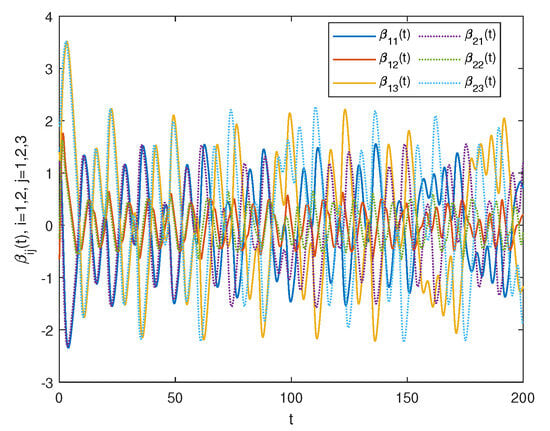
Figure 1.
Response of Example 1 when .
Set , , , , and
and
Then, it yields ,
and the AIA
Figure 2a shows the set of the AIA utilizing Algorithm 1. Since , Figure 2b indicates that System (6) can be locally stabilized via the quantized control with actuator saturation. That is, the local synchronization of Systems (1)–(2) can be successfully achieved.
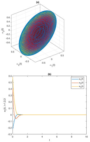
Figure 2.
(a) Set of the AIA based on Algorithm 1. (b) Trajectories of when .
4.2. Simulation Based on Algorithm 2
Example 2.
A chaotic three-neuron FONN is proposed with , , , and
thus, it can be calculated as . Take in the simulation. Then, the chaotic behavior of the drive system can be depicted, as shown in in Figure 3a,b.
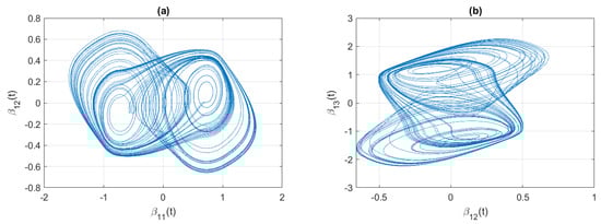
Figure 3.
Chaotic behaviors of the drive system on (a) , and (b) when .
Choose , , , , , where AIA represents the set . Through simulation, we can obtain , , , ,
and the feedback control gain
and
In the simulation, we choose to be , such that . Theorem 1 guarantees local stability for closed-loop FONNs, as shown in Figure 4. We denote the interval parameters as , , and , respectively. Table 1 presents the related minimal actuator size with the above . It is observed that as increases, also increases. However, a larger can help save energy resources by minimizing the amount of quantitative data transmitted to the controller. Therefore, a compromise can be achieved by selecting appropriate parameters that satisfy the desired requirements in engineering applications.
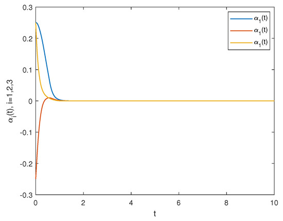
Figure 4.
Responses of when .

Table 1.
Minimum size of for different .
5. Conclusions
In this paper, we have investigated the local synchronization problem of FONNs with actuator saturation within the framework of quantized control. An RSC was established based on the features of quantizers and actuator saturation. Using fractional-order theory, we developed a sufficient condition for addressing the local synchronization issue. Two optimization algorithms were presented to maximize the AIA and minimize the actuator’s costs, respectively. Finally, we provided a demonstration of the proposed control scheme using a three-neuron FONN. The results show the validity and effectiveness of the proposed approach.
In the future, we will focus on the semi-global synchronization issue of FONNs under quantized control with actuator saturation. This is a challenging problem that will require further investigation in our future research.
Author Contributions
Writing—original draft preparation, S.F.; writing—review and editing, M.L. All authors have read and agreed to the published version of the manuscript.
Funding
This research received no external funding.
Institutional Review Board Statement
Not applicable.
Informed Consent Statement
Not applicable.
Data Availability Statement
Data sharing is not applicable to this article as no datasets were generated or analyzed during the current study.
Acknowledgments
We would like to express our great appreciation to the editors and reviewers.
Conflicts of Interest
The authors declare no conflict of interest.
References
- He, W.; Luo, T.; Tang, Y.; Du, W.; Tian, Y.; Qian, F. Secure communication based on quantized synchronization of chaotic neural networks under an event-triggered strategy. IEEE Trans. Neural Netw. Learn. Syst. 2020, 31, 3334–3345. [Google Scholar] [CrossRef] [PubMed]
- Wang, L.; Jiang, S.; Ge, M.; Hu, C.; Hu, J. Finite-/fixed-time synchronization of memristor chaotic systems and image encryptio application. IEEE Trans. Circuits Syst. I Reg. Pap. 2021, 68, 4957–4969. [Google Scholar] [CrossRef]
- Chen, H.; Liang, J. Local synchronization of interconnected Boolean networks with stochastic disturbances. IEEE Trans. Neural Netw. Learn. Syst. 2020, 31, 452–463. [Google Scholar] [CrossRef]
- Kaslik, E.; Sivasundaram, S. Nonlinear dynamics and chaos in fractional-order neural networks. Neural Net. 2012, 32, 245–256. [Google Scholar] [CrossRef]
- Sajid, M.; Chaudhary, H.; Kaushik, S. Chaos controllability in non-identical complex fractional order chaotic systems via active complex synchronization technique. Axioms 2023, 12, 530. [Google Scholar] [CrossRef]
- Tural-Polat, S.N. Solution method for systems of nonlinear fractional differential equations using third kind chebyshev wavelets. Axioms 2023, 12, 546. [Google Scholar] [CrossRef]
- Huang, C.; Nie, X.; Zhao, X. Novel bifurcation results for a delayed fractional-order quaternion-valued neural network. Neural Net. 2019, 117, 67–93. [Google Scholar] [CrossRef]
- Chen, L.; Yin, H.; Wu, X. Robust dissipativity and dissipation of a class of fractional-order uncertain linear systems. IET Control Theory Appl. 2019, 13, 1454–1465. [Google Scholar] [CrossRef]
- Li, Y.; Chen, Y.; Podlubny, I. Mittag-Leffler stability of fractional order nonlinear dynamic systems. Automatica 2009, 45, 1965–1969. [Google Scholar] [CrossRef]
- Westerlund, S.; Ekstam, L. Capacitor theory. IEEE Trans. Dielect. Electron. Insul. 1994, 1, 826–839. [Google Scholar] [CrossRef]
- Agarwal, R.P.; Hristova, S.; O’Regan, D. Mittag-Leffler-type stability of BAM neural networks modeled by the generalized proportional Riemann-Liouville fractional derivative. Axioms 2023, 12, 588. [Google Scholar] [CrossRef]
- Abdelouahab, M.; Lozi, R.; Chua, L. Memfractance: A mathematical paradigm for circuit elements with memory. Int. J. Bifurc. Chaos 2014, 24, 1430023. [Google Scholar] [CrossRef]
- Lundstrom, B.; Higgs, M.; Spain, W. Fractional differentiation by neocortical pyramidal neurons. Nat. Neurosci. 2008, 11, 1335–1342. [Google Scholar] [CrossRef] [PubMed]
- Yu, J.; Hu, C.; Jiang, H.; Fan, X. Projective synchronization for fractional neural networks. Neural Net. 2014, 49, 87–95. [Google Scholar] [CrossRef] [PubMed]
- Bao, H.; Park, J.; Cao, J.D. Adaptive synchronization of fractional-order output-coupling neural networks via quantized output control. IEEE Trans. Neural Netw. Learn. Syst. 2021, 32, 3230–3239. [Google Scholar] [CrossRef]
- Ding, Z.; Zeng, Z.; Wang, L. Robust finite-time stabilization of fractional-order neural networks with discontinuous and continuous activation functions under uncertainty. IEEE Trans. Neural Netw. Learn. Syst. 2018, 29, 1477–1490. [Google Scholar] [CrossRef]
- Yang, Y.; He, Y.; Wu, M. Intermittent control strategy for synchronization of fractional-order neural networks via piecewise Lyapunov function method. J. Franklin Inst. 2019, 356, 4648–4676. [Google Scholar] [CrossRef]
- Song, X.; Man, J.; Song, S. Event-triggered synchronisation of Markovian reaction-diffusion inertial neural networks and its application in image encryption. IET Control Theory Appl. 2020, 14, 2726–2740. [Google Scholar] [CrossRef]
- Zhai, Z.; Yan, H.; Chen, S.; Zhan, X.; Zeng, H. Further results on dissipativity analysis for TS fuzzy systems based on sampled-data control. IEEE Trans. Fuzzy Syst. 2023, 31, 660–668. [Google Scholar] [CrossRef]
- Kim, H.; Park, J.; Joo, Y. Decentralized H∞ sampled-data fuzzy filter for nonlinear interconnected oscillating systems with uncertain interconnections. IEEE Trans. Fuzzy Syst. 2020, 28, 487–498. [Google Scholar] [CrossRef]
- Chen, Y.; Wang, Z.; Shen, B. Exponential dynchronization for delayed dynamical networks via intermittent control: Dealing with actuator saturations. IEEE Trans. Neural Netw. Learn. Syst. 2019, 30, 1000–1012. [Google Scholar] [CrossRef]
- Zhou, H.; Tong, S. Adaptive neural network event-triggered output-feedback containment control for nonlinear MASs with input quantization. IEEE Trans. Cybern. 2023. [Google Scholar] [CrossRef] [PubMed]
- Aravind, R.; Balasubramaniam, P. Membership-function-dependent design of quantized fuzzy sampled-data controller for Semi-Markovian jump systems with actuator faults. IEEE Trans. Fuzzy Syst. 2023, 31, 40–52. [Google Scholar] [CrossRef]
- Fu, M.; Xie, L. The sector bound approach to quantized feedback control. IEEE Trans. Autom. Control 2005, 50, 106–111. [Google Scholar]
- Zhang, S.; Yu, Y.; Yu, J. LMI conditions for global stability of fractional-order neural networks. IEEE Trans. Neural Netw. Learn. Syst. 2017, 28, 2423–2433. [Google Scholar] [CrossRef]
- Yang, Z.; Zhang, J. Global stabilization of fractional-order bidirectional associative memory neural networks with mixed time delays via adaptive feedback control. Int. J. Comput. Math. 2020, 97, 2074–2090. [Google Scholar] [CrossRef]
- Rajchakit, G.; Pratap, A.; Raja, R. Hybrid control scheme for projective lag synchronization of Riemann-Liouville sense fractional order memristive BAM neural networks with mixed delays. Mathematics 2019, 7, 759. [Google Scholar] [CrossRef]
- Rajchakit, G.; Chanthorn, P.; Kaewmesri, P. Global Mittag-Leffler stability and stabilization analysis of fractional-order quaternion-valued memristive neural networks. Mathematics 2020, 8, 42. [Google Scholar] [CrossRef]
- Gomes da Silva, M.; Tarbouriech, S. Anti-windup design with guaranteed region of stability: An LMI-based approach. IEEE Trans. Autom. Control 2005, 50, 1698–1711. [Google Scholar]
- Seuret, A.; Gomes da Silva, M. Taking into account period variations and actuator saturation in sampled-data systems. Syst. Control Lett. 2012, 61, 1286–1293. [Google Scholar] [CrossRef]
- Sang, H.; Zhao, J. Exponential synchronization and L2-gain analysis of delayed chaotic neural networks via intermittent control with actuator saturation. IEEE Trans. Neural Netw. Learn. Syst. 2019, 30, 3722–3734. [Google Scholar] [CrossRef] [PubMed]
- Podlubny, I. Fractional Differential Equations; Academic Press: Cambridge, MA, USA, 1998. [Google Scholar]
- Phat, V.N.; Thanh, N.T. New criteria for finite-time stability of nonlinear fractional-order delay systems: A Gronwall inequality approach. Appl. Math. Lett. 2018, 83, 169–175. [Google Scholar] [CrossRef]
- Lazarevic, M.; Spasic, A. Finite-time stability analysis of fractional order time-delay systems: Gronwall approach. Math. Comput. Model. 2009, 49, 475–481. [Google Scholar] [CrossRef]
Disclaimer/Publisher’s Note: The statements, opinions and data contained in all publications are solely those of the individual author(s) and contributor(s) and not of MDPI and/or the editor(s). MDPI and/or the editor(s) disclaim responsibility for any injury to people or property resulting from any ideas, methods, instructions or products referred to in the content. |
© 2023 by the authors. Licensee MDPI, Basel, Switzerland. This article is an open access article distributed under the terms and conditions of the Creative Commons Attribution (CC BY) license (https://creativecommons.org/licenses/by/4.0/).