Green Matrices, Minors and Hadamard Products

Abstract

Green matrices are interpreted as discrete version of Green functions and are used when working with inhomogeneous linear system of differential equations. This paper discusses accurate algebraic computations using a recent procedure to achieve an important factorization of these matrices with high relative accuracy and using alternative accurate methods. An algorithm to compute any minor of a Green matrix with high relative accuracy is also presented. The bidiagonal decomposition of the Hadamard product of Green matrices is obtained. Illustrative numerical examples are included.

1. Introduction

A real value $x\ne 0$ is said to be computed to HRA whenever the obtained $\hat{x}$ satisfies

$$\frac{\parallel x-\hat{x}\parallel }{\parallel x\parallel }<Cu,$$

where u is the unit round-off and C is a constant, which does not depend on either the conditioning of the corresponding problem or arithmetic precision. An algorithm can be computed to high relative accuracy (HRA) when it only uses multiplications, divisions and sums of numbers with the same sign or subtractions of initial data (cf. [1]). In other words, the only operation that breaks HRA is the sum of numbers with opposite signs. In fact, this computation keeps HRA for initial and exact data if the floating-point arithmetic is well-implemented. The problem of obtaining an adequate parameterization of the considered classes of matrices is the cornerstone to devise HRA algorithms. A matrix is said to be totally positive (TP) if all its minors are greater than or equal to zero and it is said to be strictly totally positive (STP) if they are greater than zero (see [2,3,4]). In the literature some authors have also called TP and STP matrices as totally nonnegative and totally positive matrices, respectively (see [5]). TP matrices emerge in many applications in Approximation Theory, Statistics, Combinatory, Differential Equations or Economy (cf. [2,3,4,5,6]) and, in particular, in connection with optimal bases in Computer Aided Geometric Design (cf. [7,8]). HRA algorithms have been developed for some classes of matrices. Among them, first we mention here some few subclasses of nonsingular TP matrices and matrices related with them. For instance, for Generalized Vandermonde matrices [9], for Bernstein-Vandermonde matrices [10,11,12], for Said-Ball-Vandermonde matrices [13], for Cauchy-Vandermonde matrices [14], for Schoenmakers-Coffey matrices [15], for h-Bernstein-Vandermonde matrices [16] or for tridiagonal Toeplitz matrices [17], and much more subclasses of TP matrices. HRA algorithms for some algebraic problems related with other class of matrices have also been developed. For example, in [18] an HRA algorithm for the computation of the singular values was devised for a class of negative matrices. In [19] the authors develop a method to solve linear systems associated with a wide class of rank-structured matrices with HRA. These matrices contain the well-known Vandermonde and Cauchy matrices.

If the bidiagonal decomposition, $\mathcal{BD}\left(A\right)$, of a nonsingular TP matrix A is known to HRA, then many algebraic computations can be carried out with HRA by using the functions in the software library [20]. For instance, computing its eigenvalues, its singular values, its inverse and the solution of linear systems $Ax=b$, where b has alternating signs. In [21] a method to get bidiagonal factorizations of Green matrices to HRA with $\mathcal{O}\left(n\right)$ elementary operations was introduced. Now we shall deepen on this method and its consequences as well as we shall show alternative accurate methods for Green matrices and provide further properties of these matrices. Green matrices (see [2,3,22]) are usually interpreted as discrete version of Green functions (see p. 237 of [22]) and are used when working with inhomogeneous systems of of differential equations. Green functions emerge in the Sturm-Liouville boundary-value problem. They have important applications in many scientific fields, such as Mechanics (see [22]) or Econometrics (see [23]).

Schoenmakers-Coffey matrices form a subclass of Green matrices with important financial applications (see [24,25,26,27,28,29]). In [15] Schoenmakers-Coffey matrices were characterized by a parametrization containing n parameters. The parametrization was used in [15] to perform HRA algebraic computations. In [21], a parametrization of $2n$ parameters leading to HRA computations for nonsingular TP Green matrices was presented. In Section 2, devoted to basic notations and auxiliary results, we recall this parametrization and, in the general case of nonsingular Green matrices, we also use it in Section 3 (in Theorem 4) to obtain alternative methods to compute the determinant and the inverse with HRA. In Section 4 we provide a method to compute all minors of a Green matrix with HRA. In Section 5, the bidiagonal factorization of the Hadamard product of Green matrices is obtained. In contrast to the Hadamard product of nonsingular Green matrices, we also prove that the the Hadamard product of nonsingular TP Green matrices is also a nonsingular TP Green matrix. Section 6 includes a family of numerical experiments confirming the advantages of using the HRA methods. Finally, Section 7 summarizes the conclusions of the paper.

2. Basic Notations and Auxilliary Results

A desirable goal in the construction of numerical algorithms is the high relative accuracy (cf. [30,31]). This goal has only been achieved for a few classes of matrices. We say that an algorithm for the solution of an algebraic problem is performed to high relative accuracy in floating point arithmetic if the relative errors in the computations have the order of the unit round-off (or machine precision), without being affected by the dimension or the conventional conditionings of the problem (see [31]). It is well known that algorithms to high relative accuracy are those avoiding subtractive cancellations, that is, only requiring the following arithmetics operations: products, quotients, and additions of numbers of the same sign (see p. 52 in [1]). Moreover, if the floating-point arithmetic is well-implemented, the subtraction of initial data can also be done without loosing high relative accuracy (see p. 53 in [1]).

As mentioned in the Introduction, computations to high relative accuracy with totally positive matrices can be achieved by means of a proper representation of the matrices in terms of bidiagonal factorizations, which is in turn closely related to their Neville elimination (cf. [32,33]). Roughly speaking, Neville elimination is a procedure to make zeros in a column of a given matrix $A\in {\mathbb{R}}^{n\times n}$ by adding to each row an appropriate multiple of the previous one.

Given $A\in {\mathbb{R}}^{n\times n}$, Neville elimination consists of $n-1$ major steps

$$A=:A^{\left(1\right)}\to {\tilde{A}}^{\left(1\right)}\to A^{\left(2\right)}\to {\tilde{A}}^{\left(2\right)}\to \cdots \to A^{\left(n\right)}=:U,$$

where U is an upper triangular matrix. Every major step in turn consists of two steps. In the first of these two steps, the Neville elimination obtains ${\tilde{A}}^{\left(k\right)}$ from the matrix $A^{\left(k\right)}$ by moving to the bottom the rows with a zero entry in column k below the main diagonal, if necessary. Then, in the second step the matrix $A^{(k+1)}$ is obtained from ${\tilde{A}}^{\left(k\right)}$ according to the following formula

$$a_{i,j}^{(k+1)}:=\left\{\begin{array}{cc}{\tilde{a}}_{i,j}^{\left(k\right)},\hfill & \mathrm{if}1\le i\le k,\hfill \\ {\tilde{a}}_{i,j}^{\left(k\right)}-\frac{{\tilde{a}}_{i,k}^{\left(k\right)}}{{\tilde{a}}_{i-1,k}^{\left(k\right)}}{\tilde{a}}_{i-1,j}^{\left(k\right)},\hfill & \mathrm{if}k+1\le i,j\le n, \mathrm{and} {\tilde{a}}_{i-1,j}^{\left(k\right)}\ne 0,\hfill \\ {\tilde{a}}_{i,j}^{\left(k\right)},\hfill & \mathrm{if}k+1\le i\le n, \mathrm{and} {\tilde{a}}_{i-1,k}^{\left(k\right)}=0.\hfill \end{array}\right.$$

(1)

The process finishes when $U:=A^{\left(n\right)}$ is an upper triangular matrix. The entry

$$p_{i,j}:=a_{i,j}^{\left(j\right)},1\le j\le i\le n,$$

(2)

is the $(i,j)$ pivot and $p_{i,i}$ is called the i-th diagonal pivot of the Neville elimination of A. The Neville elimination of A can be performed without row exchanges if all the pivots are nonzero. Then the value

$$m_{i,j}:=a_{i,j}^{\left(j\right)}/a_{i-1,j}^{\left(j\right)}=p_{i,j}/p_{i-1,j},1\le j<i\le n,$$

(3)

is called the $(i,j)$ multiplier. The complete Neville elimination of A consists of performing the Neville elimination to obtain the upper triangular matrix $U=A^{\left(n\right)}$ and next, the Neville elimination of the lower triangular matrix $U^T$.

Neville elimination is an important tool to analyze if a given matrix is STP, as shown in this characterization derived from Theorem 4.1 and Corollary 5.5 of [32], and the arguments of p. 116 of [34].

Theorem 1. 

Let A be a nonsingular matrix. A is STP (resp., TP) if and only if the Neville elimination of A and $A^T$ can be performed without row exchanges, all the multipliers of the Neville elimination of A and $A^T$ are positive (resp., nonnegative), and the diagonal pivots of the Neville elimination of A are all positive.

In [34], it is shown that a nonsingular totally positive matrix $A\in {\mathbb{R}}^{n\times n}$ can be decomposed as follows,  

$$A=F_{n-1}{F}_{n-2}\cdots F_{1}D{G}_1{G}_2\cdots G_{n-1},$$

(4)

where $F_i\in {\mathbb{R}}^{n\times n}$ (respectively, $G_i\in {\mathbb{R}}^{n\times n}$) is the TP, lower (respectively, upper) triangular bidiagonal matrix given by

$$F_i=\left(\begin{array}{c}1\\ & \ddots \\ & & 1\\ & & m_{i+1,1}& 1\\ & & & \ddots & \ddots \\ & & & & m_{n,n-i}& 1\end{array}\right),$$

(5)

$$G_i^T=\left(\begin{array}{c}1\\ & \ddots \\ & & 1\\ & & {\tilde{m}}_{i+1,1}& 1\\ & & & \ddots & \ddots \\ & & & & {\tilde{m}}_{n,n-i}& 1\end{array}\right)$$

(6)

and D is a diagonal matrix whose diagonal entries are $p_{i,i}>0$, $i=1,\dots ,n$. The diagonal elements $p_{i,i}$ are the diagonal pivots of the Neville elimination of A. Moreover, the elements $m_{i,j}$ and ${\tilde{m}}_{i,j}$ are the multipliers of the Neville elimination of A and $A^T$, respectively. The bidiagonal factorization of (4) is usually compacted in matrix form $\mathcal{BD}\left(A\right)$ as follows

$${\left(\mathcal{BD}\left(A\right)\right)}_{ij}=\left\{\begin{array}{cc}{m}_{i,j},\hfill & \mathrm{for}1\le j<i\le n,\hfill \\ {\tilde{m}}_{j,i},\hfill & \mathrm{for}1\le i<j\le n,\hfill \\ p_{i,i},\hfill & \mathrm{for}i=j\in \{1,\dots ,n\}.\hfill \end{array}\right.$$

The transpose of a nonsingular totally positive matrix A is also totally positive and, using the factorization (4), it can be written as follows

$$A^T=G_{n-1}^T{G}_{n-2}^T\cdots G_1^{T}D{F}_1^T{F}_2^T\cdots F_{n-1}^T.$$

If, in addition, A is symmetric, then we have that $G_i=F_i^T$, $i=1,\dots ,n-1$, and then

$$A=F_{n-1}{F}_{n-2}\cdots F_{1}D{F}_1^T{F}_2^T\cdots F_{n-1}^T,$$

(7)

where $F_i$, $i=1,\dots ,n-1$, are the lower triangular bidiagonal matrices described in (5), whose off-diagonal entries coincide with the multipliers of the Neville elimination of A and D is the diagonal matrix with the diagonal pivots of the Neville elimination of A.

Under certain conditions (cf. [34]), the factorization (4) is unique. On the other hand, Neville elimination can also allow us to obtain bidiagonal factorizations as in (4) for some matrices that are singular and that are not TP. This will happen in the following sections. When the matrix is singular some diagonal entries of the matrix D of (4) can be zero.

Many of the subclasses of TP matrices mentioned in the introduction are very ill-conditioned, so that classical error analysis (cf. [35]) expects great roundoff errors when performing algebraic calculations with those matrices. However, the parametrization provided by the bidiagonal decomposition allows us to compute many algebraic calculations with high relative accuracy. Let us recall that, given a nonsingular and totally positive matrix A, by providing its bidiagonal factorization $B=\mathcal{BD}\left(A\right)$ to high relative accuracy, the Matlab functions avalaible in the software library TNTools in [20] compute to high relative accuracy $A^{-1}$ (using the algorithm presented in [36]), the solution of $Ax=b$, for vectors b with alternating signs, and the singular values of A, which coincide with the eigenvalues when the matrix is also symmetric, as it happens with Green matrices. In particular:

• TNInverseExpand$\left(B\right)$ returns $A^{-1}$, requiring $O(n^2$) elementary operations.
• TNSolve$(B,d)$ returns the solution c of $Ac=d$. It requires $O(n^2$) elementary operations.
• TNSingularValues(B) returns the singular values of A. Its computational cost is $O\left(n^3\right)$.

Following [4], we are going to recall the definition of a Green matrix. Given two sequences of nonzero real numbers ${\left(u_i\right)}_{1\le i\le n}$, ${\left(v_i\right)}_{1\le i\le n}$, a Green matrix $A={\left(a_{ij}\right)}_{1\le i,j\le n}$ is the symmetric matrix given by $a_{ij}=u_i{v}_j$ if $i\le j$ (or, equivalently, $a_{ij}=u_{min\{i,j\}}{v}_{max\{i,j\}}$ for all $i,j$).

The initial parameters used in [21] to get HRA algorithms were:

$$v_i,r_i:=\frac{u_i}{v_i},i=1,\dots ,n.$$

(8)

Then, the elements of the Green matrix $A={\left(a_{ij}\right)}_{1\le i,j\le n}$ can be expressed as $a_{ij}=r_i{v}_i{v}_j$ for $i\le j$. We also have that $u_i=v_i{r}_i$ for all $i=1,\dots ,n$.

In Theorem 4.2 of [4] or p. 214 of [2] a result characterizing TP Green matrices was presented. Let us now recall it. Using (8), it can be stated as follows.

Theorem 2. 

A Green matrix is TP if and only if the parameters (8) are formed by numbers of the same stric sign and   

$$(0<)r_1\le \cdots \le r_n.$$

(9)

The parameters (8) can be seen as natural parameters for a Green matrix taking into account Theorem 2 and the characterization of nonsingular Green matrices that we shall show below in Section 3.

Recently, a bidiagonal factorization of a Green matrix A to HRA has been derived. Let us now recall this decomposition of A. Using it, when A is also nonsingular TP, we can also carry out some algebraic computations of A to HRA: computation of its eigenvalues (which coincide with its singular values by the symmetry of the matrix), of its inverse and of the solution of some linear systems. Although this result is presented in [21], we include it with its proof for the sake of completeness.

Theorem 3. 

Let A be a Green matrix where the parameters (8) are known. Then, the bidiagonal factorization $\mathcal{BD}\left(A\right)$ of A can be computed to HRA. If, in addition, A is nonsingular TP, then its eigenvalues, $A^{-1}$ and the solution of linear systems $Ax=b$ (where b has alternating signs) can also be computed with HRA.

Proof. 

The result in [21] was proved by systematically applying complete Neville elimination to A and keeping track the corresponding steps in matrix form. So, the first major step of the complete Neville elimination (it makes zeros the entries $(n,1)$ and $(1,n)$ by performing row an column matrix elementary operations) was expressed in matrix form as

$$E_n\left(\frac{-v_n}{v_{n-1}}\right)A{E}_n{\left(\frac{-v_n}{v_{n-1}}\right)}^T=M,$$

where $E_i\left(\alpha \right)$ ($2\le i\le n$) denotes the elementary matrix coinciding with the order $n\times n$ identity matrix except for the place $(i,i-1)$, which is $\alpha$ instead of 0. With respect to the matrix M, all the elements of its last row and its last column are zero except for the entry $(n,n)$, which is given by

$$d_n:=v_n^2(r_n-r_{n-1}).$$

(10)

Performing the major steps $2,\dots ,n-1$ of the complete Neville elimination to convert the entries $(n-1,1)$, $(1,n-1),\dots ,(2,1)$, $(1,2)$ to zeros, the following factorization was obtained

$$E_2\left(\frac{-v_2}{v_1}\right)\cdots E_n\left(\frac{-v_n}{v_{n-1}}\right)A{E}_n{\left(\frac{-v_n}{v_{n-1}}\right)}^T\cdots E_2{\left(\frac{-v_2}{v_1}\right)}^T=D,$$

(11)

where $D=diag(d_1,\dots ,d_n)$ is the diagonal matrix given by

$$d_1=r_1{v}_1^2,d_i=v_i^2(r_i-r_{i-1}),i>1.$$

(12)

From (11) the following factorization of A was deduced

$$A=E_n\left(\frac{v_n}{v_{n-1}}\right)\cdots E_2\left(\frac{v_2}{v_1}\right)D{E}_2{\left(\frac{v_2}{v_1}\right)}^T\cdots E_n{\left(\frac{v_n}{v_{n-1}}\right)}^T,$$

(13)

that is, $\mathcal{BD}\left(A\right)$. Observe that all elements of the decomposition (13) can be obtained with HRA.

If A is a nonsingular and totally positive matrix, by using the algorithms devised in [36,37], the announced algebraic computations can be carried out to HRA from the bidiagonal factorization of A. □

Observe in the proof of the previous result that the only nonzero entries of the compacted matrix form of the bidiagonal factorization (commented above) of a Green matrix lie in the first row, the first column or the diagonal.

In Remark 2.2 of [21] we discussed the computational cost of the algorithm given in the proof of Theorem 3 and taking into account the computational costs of the algorithms given in [36,37], the computational cost of its application to compute the eigenvalues, the inverse or the solution of a linear system of equations for a Green matrix.

3. Accurate Method for the Inverse and Determinant of a Green Matrix

The next result is valid for all nonsingular Green matrices, which are characterized in terms of the parameters (8). For nonsingular TP Green matrices, it also provides an alternative way to that of Theorem 3 for calculating their inverses with HRA.

Theorem 4. 

A Green matrix $A={\left(a_{ij}\right)}_{1\le i,j\le n}$ is nonsingular if and only if the parameters $r_i$ of (8) satisfy that $r_i\ne r_{i+1}$ for all $i=1,\dots ,n-1$. In this case, if we know the parameters (8), then we can compute $detA$ and $A^{-1}$ with HRA and $\mathcal{O}\left(n\right)$ elementary operations.

Proof. 

With the notations of the proof of Theorem 3, observe that the matrix

$$U:=D{E}_2{\left(\frac{v_2}{v_1}\right)}^T\cdots E_n{\left(\frac{v_n}{v_{n-1}}\right)}^T$$

is upper triangular, it has as diagonal entries $d_i$ ($i=1,\dots ,n$) given by (12) and

$$detA=detU={\Pi }_{i=1}^n{d}_i.$$

(14)

Therefore, if we know the parameters (8), then we can compute $detA$ by (12) and (14) with HRA and the computational cost is $\mathcal{O}\left(n\right)$ elementary operations. Besides, Equation (14) also implies that $detA\ne 0$ if and only if $d_i\ne 0$ for all $i=1,\dots ,n$, which is equivalent by (12) to the fact that $r_i\ne r_{i+1}$ for all $i=1,\dots ,n-1$.

Besides, if we know the parameters (8), then we can also compute the parameters $u_i=v_i{r}_i$ with HRA for all $i=1,\dots ,n$. Finally, in the nonsingular case of $A={\left(a_{ij}\right)}_{1\le i,j\le n}$ with $a_{ij}=u_i{v}_j$ if $i\le j$, by Theorem 1 of [15] its inverse $C=G^{-1}={\left(c_{ij}\right)}_{1\le i,j\le n}$ is the tridiagonal matrix given by

$$\begin{array}{cc}\hfill c_{11}& =\frac{u_2}{u_1(u_2{v}_1-u_1{v}_2)}=\frac{v_2{r}_2}{v_1{r}_1(u_2{v}_1-u_1{v}_2)},\hfill \\ \hfill c_{ii}& =\frac{u_{i+1}{v}_{i-1}-u_{i-1}{v}_{i+1}}{(u_i{v}_{i-1}-u_{i-1}{v}_i)(u_{i+1}{v}_i-u_i{v}_{i+1})},i=2,\dots ,n-1,\hfill \\ \hfill c_{nn}& =\frac{v_{n-1}}{v_n(u_n{v}_{n-1}-u_{n-1}{v}_n)},\hfill \\ \hfill c_{i+1,i}=c_{i,i+1}& =\frac{1}{u_i{v}_{i+1}-u_{i+1}{v}_i},i=1,\dots ,n-1.\hfill \end{array}$$

Observe that, for $i=2,\dots ,n$,

$$u_i{v}_{i-1}-v_i{u}_{i-1}=r_i{v}_i{v}_{i-1}-v_i{r}_{i-1}{v}_{i-1}=v_{i-1}{v}_i(r_i-r_{i-1})$$

(15)

and, for $i=2,\dots ,n-1$,

$$u_{i+1}{v}_{i-1}-v_{i+1}{u}_{i-1}=r_{i+1}{v}_{i+1}{v}_{i-1}-v_{i+1}{r}_{i-1}{v}_{i-1}=v_{i-1}{v}_{i+1}(r_{i+1}-r_{i-1}).$$

(16)

If we know the parameters (8), then we can compute (15) and (16) with HRA and so $A^{-1}$ with HRA and with a computational cost of $\mathcal{O}\left(n\right)$ elementary operations. □

Observe that the proof of Theorem 4 also provides accurately the null determinant when the Green matrix is singular because, in this case, one of the pivots $d_i$ is zero and so $det\left(A\right)=0$ by (14).

Recall that a TP matrix is oscillatory if a certain power $A^k$ is STP. The following remark shows that, if we have a nonsingular and TP Green matrix A, then A is oscillatory.

Remark 1. 

Taking into account Theorems 3 and 4, when the inequalities of (9) are strict then we have a nonsingular TP matrix $A={\left(a_{ij}\right)}_{1\le i,j\le n}$. In fact, since all entries $a_{i,i+1}=u_i{v}_{i+1}=a_{i+1,i}$ are nonzero ($i=1,\dots ,n-1$), then by Theorem 4.2 of [2] A is oscillatory. Remember (cf. Theorem 6.5 of [2]) that an oscillatory matrix has all its eigenvalues distinct and positive.

4. Accurate Method for the Minors of a Green Matrix

Let $A={\left(a_{ij}\right)}_{1\le i,j\le n}$ be a real square matrix and k a positive integer satisfying $k\le n$. With $Q_{k,n}$ will be denoted the set of all strictly increasing sequences of k natural numbers less than or equal to n:

$$\alpha ={\left({\alpha }_i\right)}_{i=1}^k\in Q_{k,n}\mathrm{if}(1\le ){\alpha }_1<{\alpha }_2<\dots <{\alpha }_k\left(\le n\right)·$$

Given $\alpha ,\beta \in Q_{k,n}$, then $A\left[\alpha \right|\beta ]$ is by definition the $k\times k$ submatrix of A containing rows numbered by $\alpha$ and columns numbered by $\beta$.

As shown in p. 4 of [15], a Green matrix $A={\left(a_{ij}\right)}_{1\le i,j\le n}$ ($n\ge 3$) cannot be strictly totally positive because it always has zero minors. In fact, for any $i,j$ with $i<j(<n)$, $detA[i,i+1|j,j+1]=u_i{v}_j{u}_{i+1}{v}_{i+1}-u_i{v}_{i+1}{v}_j{u}_{i+1}=0$. The following result will show that we can compute all minors of a Green matrix with high relative accuracy. Its proof includes an explicit formula for the computation of nonzero minors that can be performed with high relative accuracy.

Theorem 5. 

If $A={\left(a_{ij}\right)}_{1\le i,j\le n}$ is a Green matrix with known parameters (8), then we can compute any minor of A with HRA.

Proof. 

As proved in pp. 110–111 of [3], any minor $detA[i_1,\dots ,i_p|j_1,\dots ,j_p]$ of a Green matrix A satisfies

$$\begin{array}{c}detA[i_1,\dots ,i_p|j_1,\dots ,j_p]\hfill \\ =u_{k_1}\times det\left(\begin{array}{cc}{u}_{k_2}& u_{h_1}\\ v_{k_2}& v_{h_1}\end{array}\right)det\left(\begin{array}{cc}{u}_{k_3}& u_{h_2}\\ v_{k_3}& v_{h_2}\end{array}\right)\cdots det\left(\begin{array}{cc}{u}_{k_p}& u_{h_{p-1}}\\ v_{k_p}& v_{h_{p-1}}\end{array}\right)\times v_{h_p}\hfill \end{array}$$

(17)

where $k_m=min(i_m,j_m)$ and $h_m=max(i_m,j_m)$, provided $i_m,j_m<i_{m+1},j_{m+1}$ ($m=1,2,\dots ,p-1$). In all other cases, the minor is zero.

Taking into account that $u_{k_1}=r_{k_1}{v}_{k_1}$ and that, for each $m=2,\dots ,p-1$,

$$det\left(\begin{array}{cc}{u}_{k_m}& u_{h_{m-1}}\\ v_{k_m}& v_{h_{m-1}}\end{array}\right)=u_{k_m}{v}_{h_{m-1}}-v_{k_m}{u}_{h_{m-1}}=v_{h_{m-1}}{v}_{k_m}(r_{k_m}-r_{h_{m-1}}),$$

(18)

we can deduce from (17) that all nonzero minors of A can be calculated as

$$detA[i_1,\dots ,i_p|j_1,\dots ,j_p]=r_{k_1}{v}_{k_1}{v}_{h_p}\prod _{m=2}^{p-1}\left(v_{h_{m-1}}{v}_{k_m}(r_{k_m}-r_{h_{m-1}})\right)$$

(19)

We can observe that, with the initial parameters (8), the calculation of (19) can be performed with HRA. □

5. Hadamard Product of Green Matrices

Given two $n\times m$ matrices $A=\left(a_{ij}\right)$ and $B=\left(b_{ij}\right)$ the Hadamard (or entrywise) product of A and B is the $n\times m$ matrix $C=A\circ B$ defined by $c_{ij}=a_{ij}{b}_{ij}$. There are some properties of the ordinary product of totally positive matrices that do not hold for the Hadamard product. A first property is the fact that the product of two totally positive matrices is totally positive (see Theorem 3.1 of [2]). However, in general, the class of totally positive matrices is not closed under the operation of Hadamard products (see p. 120 of [4]). For instance, consider the $3\times 3$ TP matrix A with 0 in entry $(1,3)$ and 1 elsewhere. Then A and $A^T$ are TP, but $A\circ A^T$ has determinant $-1$ and so it is not TP. Let us see this counterexample with more detail:

$$A\circ A^T=\left(\begin{array}{ccc}1& 1& 0\\ 1& 1& 1\\ 1& 1& 1\end{array}\right)\circ \left(\begin{array}{ccc}1& 1& 1\\ 1& 1& 1\\ 0& 1& 1\end{array}\right)=\left(\begin{array}{ccc}1& 1& 0\\ 1& 1& 1\\ 0& 1& 1\end{array}\right)$$

and then  

$$det(A\circ A^T)=det\left(\begin{array}{ccc}1& 1& 0\\ 1& 1& 1\\ 0& 1& 1\end{array}\right)=-1.$$

However, the Hadamard product of totally positive Green matrices is a totally positive Green matrix (see p. 120 of [4]).

The second announced property deals with the bidiagonal factorization. If we know the bidiagonal factorizations $\mathcal{BD}\left(A\right)$ and $\mathcal{BD}\left(B\right)$ of two nonsingular totally positive matrices A and B, then we can find in [37] a method to obtain the bidiagonal factorization $\mathcal{BD}\left(AB\right)$ of their ordinary product $AB$. This method has not been extended to the Hadamard product. However, we are going to see that, if we know the parameters (8) of two Green matrices, then we can obtain the bidiagonal factorization (4) of their Hadamard product.

Theorem 6. 

If A and B are $n\times n$ Green matrices with parameters (8) given by $v_i^A$, $r_i^A$ and $v_i^B$, $r_i^B$, respectively, then the bidiagonal factorization of the Hadamard product $A\circ B$ is given by

$$A\circ B=E_n\left(\frac{v_n^A·v_n^B}{v_{n-1}^A·v_{n-1}^B}\right)\cdots E_2\left(\frac{v_2^A·v_2^B}{v_1^A·v_1^B}\right)D{E}_2{\left(\frac{v_2^A·v_2^B}{v_1^A·v_1^B}\right)}^T\cdots E_n{\left(\frac{v_n^A·v_n^B}{v_{n-1}^A·v_{n-1}^B}\right)}^T,$$

where $D=diag(d_1,\dots ,d_n)$ is matrix given by

$$d_1=r_1^A{\left(v_1^A\right)}^2{r}_1^B{\left(v_1^B\right)}^2,d_i={\left(v_i^A\right)}^2{\left(v_i^B\right)}^2(r_i^A{r}_i^B-r_{i-1}^A{r}_{i-1}^B)i>1.$$

(20)

Proof. 

Neville elimination must be performed. First, $(v_n^A·v_n^B)/(v_{n-1}^A·v_{n-1}^B)$ times the last but one row is substracted to the last row in order to transform the place $(n,1)$ of $A\circ B$ to zero. Like in the case of the Neville elimination on a Green matrix, this elementary operation also converts the remaining off-diagonal elements of the last row to zero. After carrying out the previous operation, the $(n,n)$ place of $A\circ B$ is transformed to

$$\begin{array}{cc}\hfill d_n:& =r_n^A{\left(v_n^A\right)}^2{r}_n^B{\left(v_n^B\right)}^2-\frac{v_n^A{v}_n^B}{v_{n-1}^A{v}_{n-1}^B}{r}_{n-1}^A{v}_{n-1}^A{v}_n^A{r}_{n-1}^B{v}_{n-1}^B{v}_n^B\hfill \\ \hfill & ={\left(v_n^A\right)}^2{\left(v_n^B\right)}^2\left(r_n^A{r}_n^B-r_{n-1}^A{r}_{n-1}^B\right).\hfill \end{array}$$

By symmetry, if $(v_n^A·v_n^B)/(v_{n-1}^A·v_{n-1}^B)$ times the last but one column is subtracted to the last column, a matrix, where all the entries of the last column up to the place $(n,n)$ are zero, is obtained. The entry $(n,n)$ does not change and $d_n$ remains. So, this first major step can be expressed in matrix form as

$$E_n\left(\frac{-v_n^A{v}_n^B}{v_{n-1}^A{v}_{n-1}^B}\right)(A\circ B)E_n{\left(\frac{-v_n^A{v}_n^B}{v_{n-1}^A{v}_{n-1}^B}\right)}^T=M$$

If this process is continued to transform the entries $(n-1,1),(1,n-1),\dots ,(2,1),(1,2)$ to zeros, the following decomposition is obtained   

$$E_2\left(\frac{-v_2^A{v}_2^B}{v_1^A{v}_1^B}\right)\cdots E_n\left(\frac{-v_n^A{v}_n^B}{v_{n-1}^A{v}_{n-1}^B}\right)(A\circ B)E_n{\left(\frac{-v_n^A{v}_n^B}{v_{n-1}^A{v}_{n-1}^B}\right)}^T\cdots E_2{\left(\frac{-v_2^A{v}_2^B}{v_1^A{v}_1^B}\right)}^T=D,$$

(21)

where D is the diagonal matrix with diagonal entries in (20).

Taking into account the formula for the inverse of $E_i\left(\alpha \right)$, the following bidiagonal factorization $\mathcal{BD}(A\circ B)$ of $A\circ B$ is obtained:

$$A\circ B=E_n\left(\frac{v_n^A{v}_n^B}{v_{n-1}^A{v}_{n-1}^B}\right)\cdots E_2\left(\frac{v_2^A{v}_2^B}{v_1^A{v}_1^B}\right)D{E}_2{\left(\frac{v_2^A{v}_2^B}{v_1^A{v}_1^B}\right)}^T\cdots E_n{\left(\frac{v_n^A{v}_n^B}{v_{n-1}^A{v}_{n-1}^B}\right)}^T.$$

 □

Observe that Theorem 6 does not require any additional property for the Green matrices that are factors of the Hadamard product: neither total positivity neither singularity.

Remark 2. 

As recalled above, the Hadamard product of two totally positive Green matrices is a totally positive Green matrix. However, the Hadamard product of nonsingular Green matrices can be singular. Now let us illustrate this with an example. Let us consider two nonsingular Green matrices A and B given by the sequences $r^A=\{3,5\}$, $v^A=\{1/3,1/5\}$ and $r^B=\{5,3\}$, $v^B=\{1/5,1/3\}$. The Green matrices A and B can be written explicitly as

$$A=\left(\begin{array}{cc}\frac{1}{3}& \frac{1}{5}\\ \frac{1}{5}& \frac{1}{5}\end{array}\right)andB=\left(\begin{array}{cc}\frac{1}{5}& \frac{1}{3}\\ \frac{1}{3}& \frac{1}{3}\end{array}\right).$$

We can observe that A and B are both nonsingular. In contrast, the Hadamard product of A and B  

$$A\circ B=\left(\begin{array}{cc}\frac{1}{15}& \frac{1}{15}\\ \frac{1}{15}& \frac{1}{15}\end{array}\right)$$

is clearly singular.

In contrast to the previous remark, the next result will show that the Hadamard product of two nonsingular TP Green matrices is again a nonsingular TP Green matrix.

Theorem 7. 

If A and B are $n\times n$ nonsingular TP Green matrices, then the Hadamard product $A\circ B$ is also a nonsingular TP Green matrix.

Proof. 

It is known that the Hadamard product of totally positive Green matrices is a totally positive Green matrix (see p. 120 of [4]). Let $v_i^A$, $r_i^A$ and $v_i^B$, $r_i^B$ ($i=1,\dots ,n$) be the parameters (8) of A and B, respectively. Since A and B are totally positive, by Theorem 2 we have that $(0<)r_1^A\le \cdots \le r_n^A$ and that $(0<)r_1^B\le \cdots \le r_n^B$ and since they are also nonsingular, we deduce from Theorem 4 that

$$(0<)r_1^A<\cdots <r_n^A,(0<)r_1^B<\cdots <r_n^B.$$

(22)

Taking into account the bidiagonal factorization of a Green matrix given in Theorem 3 and the bidiagonal factorization of the Hadamard product of Green matrices given in Theorem 6, we deduce that the parameters $r_i^{A\circ B}$ of $A\circ B$ are given by $r_i^{A\circ B}=r_i^A{r}_i^B$. Then, by (22), $r_i^{A\circ B}<r_{i+1}^{A\circ B}$ for all $i=1,\dots ,n-1$ and so, by Theorem 4, we deduce that $A\circ B$ is nonsingular. □

6. Numerical Tests

Given an square nonsingular TP matrix A, if the bidiagonal decomposition $\mathcal{BD}\left(A\right)$ of A is known to HRA, Koev ([37,38]) developed HRA algorithms to perform the following algebraic tasks:

• computation of the eigenvalues of A,
• computation of the singular values of A, and
• computation of the solution of linear systems of equations $Ax=b$, where b has an alternating sign pattern.

These methods were implemented by Koev in the software library TNTool available for download in [20] for the MATLAB and Octave environment. The corresponding functions are TNEigenvalues, TNSingularValues, and TNSolve, respectively. In addition, in [36] an algorithm to compute the inverse of A was developed. This algorithm was implemented by the authors in the function TNInverseExpand and contributed to the software library [20]. The previous four functions require as input argument $\mathcal{BD}\left(A\right)$ to HRA and, for the case of TNSolve, the vector b of the linear system $Ax=b$ to be solved is also necessary as second argument.

In the proof of Theorem 3 the bidiagonal decomposition of a Green matrix was recalled. The corresponding method to obtain this bidiagonal decomposition was implemented in a Matlab/Octave function TNBDGreen to be used together with the software library [20]. In Algorithm 1 we can see the pseudocode of this function.

Algorithm 1 Computation of the bidiagonal decomposition of a Green matrix A

Require: ${\left(v\left(i\right)\right)}_{i=1}^n$ and ${\left(r\left(i\right)\right)}_{i=1}^n$

Ensure: B bidiagonal decomposition of A

$B(1,1)=r\left(1\right)\ast v{\left(1\right)}^2$

for $i=2:n$ do

$B(i,1)=v\left(i\right)/v(i-1)$

$B(1,i)=v\left(i\right)/v(i-1)$

$B(i,i)=v{\left(i\right)}^2\ast (r\left(i\right)-r(i-1))$

end for

Now we will illustrate some of the theoretical results presented along this paper with numerical examples. First, in our numerical tests, we have considered the Green matrix $A_{30}$ of order 30 whose bidiagonal decomposition is given by the parameters $v={\left(v_i\right)}_{i=1}^{30}$ and $r={\left(r_i\right)}_{i=1}^{30}$ defined by

$$v_i=i\mathrm{and}{r}_i=1+\frac{1}{2^{40-i}}\mathrm{for}i=1,\dots ,30.$$

It is the Green matrix with parameters given by the sequence v and the sequence $u={\left(u_i\right)}_{i=1}^{30}$ defined by $u_i=i\left(1+\frac{1}{2^{40-i}}\right)$ for $i=1,\dots ,30$. By Theorem 2, the matrix $A_{30}$ is TP and, by Theorem 4, the matrix is also nonsingular. In fact, by Remark 1, $A_{30}$ is oscillatory. Then, by Theorem 3, $\mathcal{BD}\left(A_{30}\right)$ can be computed to HRA and, in addition, using this bidiagonal decomposition and the software library [20] for example the eigenvalues of $A_{30}$ can also be computed to HRA.

So the eigenvalues of $A_{30}$ has been calculated with Mathematica using a 200-digit precision. In addition, these eigenvalues have also been computed with Matlab in two different ways:

• by using the usual function eig, and
• by using the function TNEigenvalues using the bidiagonal decomposition $\mathcal{BD}\left(A_{30}\right)$ computed to HRA with TNBDGreen.

Then, in order to compare the accuracy of the approximations to the eigenvalues obtained with Matlab in these two ways (eig and TNEigenvalues) we have obtained the relative errors considering the eigenvalues obtained with Mathematica as exact. The eigenvalues of $A_{30}$ have been arranged in a decreasing order (${\lambda }_1>{\lambda }_2>\cdots >{\lambda }_{30}>0$) to illustrate the computed relative errors. In Figure 1, the relative errors of the approximation to these eigenvalues by both methods have been displayed. Although we have calculated the relative errors of both methods for a discrete number of eigenvalues, in order to improve the readability of the picture, the piecewise linear interpolant of these errors has been plotted for each method (piecewise linear interpolants have also been used in the following figures of the paper). The figure shows that using $\mathcal{BD}\left(A_{30}\right)$ to HRA together with the function TNEigenvalues of Koev software library ([20]) provides much better results than these obtained by using the usual Matlab function eig from the point of view of accuracy.

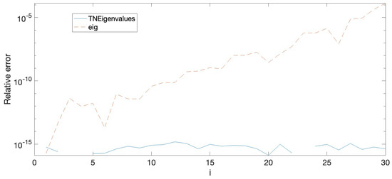
Figure 1. Relative errors when computing the eigenvalues ${\lambda }_i$, $i=1,\dots ,30$, with Matlab.

Figure 1 shows that, for the lower eigenvalues, eig Matlab command does not provide satisfactory approximations in contrast to the accurate approximations provided by the HRA bidiagonal decomposition of A joint with the function TNEigenvalues of Plamen Koev software library. Taking into account that the lowest eigenvalues present the most difficulties to be approximated, now we consider the Green matrices $A_n$, $n=6,8,\dots ,40$, of order n given by the parameters $v_n={\left(v_i^n\right)}_{i=1}^n$ and $r_n={\left(r_i^n\right)}_{i=1}^n$ defined by

$$v_i^n=i\mathrm{and}{r}_i^n=1+\frac{1}{2^{n+10-i}}\mathrm{for}i=1,\dots ,n.$$

The matrix $A_n$ corresponds to the Green matrix given by the sequence $v_n$ and the sequence $u_n={\left(u_i^n\right)}_{i=1}^{20}$ defined by $u_i^n=i\left(1+\frac{1}{2^{n+10-i}}\right)$ for $i=1,\dots ,n$. We have computed the 2-norm condition numbers of these matrices $A_n$, $n=6,8,\dots ,40$: $\kappa \left(A_n\right)=\parallel A_n{\parallel }_2·{\parallel A_n^{-1}\parallel }_2$. These condition numbers can be seen in Table 1. For a more intuitive representation of these condition numbers you can see Figure 2. Due to these huge condition numbers we cannot expect accurate enough results when performing algebraic computations by the usual methods for those matrices. In this case, algorithms taking into account the structure of the matrices are desirable in order to obtain good numerical results. Green matrices $A_n$, $n=6,8,\dots ,40$, are nonsingular TP matrices and their bidiagonal decompositions $\mathcal{BD}\left(A_n\right)$ can also be computed to HRA.

Table 1. 2-norm condition number $\kappa \left(A_n\right)$ for $n=6,8,\dots ,40$.

n	$\mathit{\kappa }\left({\mathit{A}}_{\mathit{n}}\right)$
6	$3.81388\times {10}^6$
8	$3.41953\times {10}^7$
10	$2.58123\times {10}^8$
12	$1.74308\times {10}^9$
14	$1.08872\times {10}^{10}$
16	$6.41847\times {10}^{10}$
18	$3.61933\times {10}^{11}$
20	$1.97009\times {10}^{12}$
22	$1.04201\times {10}^{13}$
24	$5.38161\times {10}^{13}$
26	$2.72417\times {10}^{14}$
28	$1.35553\times {10}^{15}$
30	$6.64583\times {10}^{15}$
32	$3.21641\times {10}^{16}$
34	$1.53904\times {10}^{17}$
36	$7.29018\times {10}^{17}$
38	$3.42223\times {10}^{18}$
40	$1.59352\times {10}^{19}$

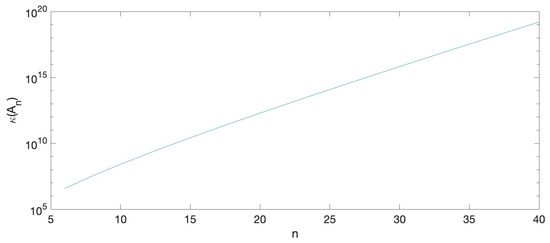
Figure 2. 2-norm condition number $\kappa \left(A_n\right)$ for $n=6,8,\dots ,40$.

Approximations of the lowest eigenvalue of these matrices by HRA methods and by Matlab command eig have been considered. Then we have computed those eigenvalues with Mathematica using a 200 digits precision. The relative errors for the approximations of the eigenvalues obtained previously have been calculated considering the eigenvalues provided by Mathematica as exact. Table 2 shows the relative errors of the approximation to the lowest eigenvalue ${\lambda }_n^n$ of each matrix $A_n$ for $n=2,4,\dots ,40$. In Figure 3 we can see these same relative errors in a graphical way.

Table 2. Relative errors when computing the eigenvalues ${\lambda }_n^n$ of $A_n$ for $n=6,8,\dots ,40$.

n	${\mathit{\lambda }}_{\mathit{n}}^{\mathit{n}}$	TNEigenvalues	eig
6	$2.3869\times {10}^{-05}$	$1.4194\times {10}^{-16}$	$1.4422\times {10}^{-12}$
8	$5.9675\times {10}^{-06}$	$2.8388\times {10}^{-16}$	$1.5301\times {10}^{-13}$
10	$1.4919\times {10}^{-06}$	$2.8388\times {10}^{-16}$	$4.6748\times {10}^{-12}$
12	$3.7297\times {10}^{-07}$	$1.4194\times {10}^{-16}$	$5.1488\times {10}^{-11}$
14	$9.3242\times {10}^{-08}$	$4.2582\times {10}^{-16}$	$9.7463\times {10}^{-10}$
16	$2.3310\times {10}^{-08}$	$8.5165\times {10}^{-16}$	$3.6172\times {10}^{-09}$
18	$5.8276\times {10}^{-09}$	$2.8388\times {10}^{-16}$	$6.3593\times {10}^{-09}$
20	$1.4569\times {10}^{-09}$	$7.0971\times {10}^{-16}$	$8.9982\times {10}^{-08}$
22	$3.6423\times {10}^{-10}$	$1.1355\times {10}^{-15}$	$1.9536\times {10}^{-07}$
24	$9.1057\times {10}^{-11}$	$2.8388\times {10}^{-16}$	$2.1620\times {10}^{-06}$
26	$2.2764\times {10}^{-11}$	$4.2582\times {10}^{-16}$	$3.5856\times {10}^{-06}$
28	$5.6910\times {10}^{-12}$	0	$6.5372\times {10}^{-06}$
30	$1.4228\times {10}^{-12}$	$4.2582\times {10}^{-16}$	$1.3889\times {10}^{-04}$
32	$3.5569\times {10}^{-13}$	$1.4194\times {10}^{-16}$	$2.3374\times {10}^{-04}$
34	$8.8922\times {10}^{-14}$	$1.4194\times {10}^{-16}$	$5.0519\times {10}^{-04}$
36	$2.2231\times {10}^{-14}$	$5.6777\times {10}^{-16}$	$5.6332\times {10}^{-03}$
38	$5.5577\times {10}^{-15}$	$1.7033\times {10}^{-15}$	$8.3078\times {10}^{-03}$
40	$1.3894\times {10}^{-15}$	$2.1291\times {10}^{-15}$	$3.3643\times {10}^{-02}$

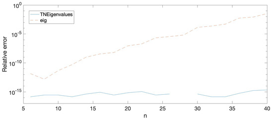
Figure 3. Relative errors when computing the eigenvalues ${\lambda }_n^n$ for $n=6,8,\dots ,40$, with Matlab.

The bidiagonal decomposition of a Green matrix A to HRA together with the functions TNInverseExpand and TNSolve of the software library [20] allow us to compute its inverse and the solution of $Ax=b$, where b has alternating signs, to HRA. Now let us compare numerically the accuracy of our HRA methods with this of the usual methods in Matlab. In this respect we have computed the inverse of the considered Green matrix of order 40, $A_{40}^{-1}$, with Mathematica using a 200-digit precision. We have also computed with Matlab the inverse $A_{40}^{-1}$ with the usual function inv and with the function TNInverseExpand using $\mathcal{BD}\left(A_{40}\right)$ to HRA obtained with the function TNBDGreen. Then we have computed the componentwise relative errors for both Matlab approximations. Finally, we have calculated the average of the componentwise relative errors for both approximations and the greatest componentwise relative error. These data can be seen in Table 3.

Table 3. Relative errors when computing $A_{40}^{-1}$.

	Maximum Rel. Error	Average Rel. Error
TNInverseExpand	$2.1988\times {10}^{-16}$	$4.8020\times {10}^{-17}$
inv	$1.0002\times {10}^{-02}$	$4.9671\times {10}^{-04}$

Now let us consider a system of linear equations $A_{40}x=b$, where b has an alternating pattern of signs with the absolute value of its entries randomly generated as integers in the interval $[1,1000]$. First we have calculated the exact solution x of the linear system with Mathematica. Then we have obtained approximations to the exact solution of the system with the usual Matlab command \ and with TNSolve of the software library [20] using the bidiagonal factorization $\mathcal{BD}\left(A_{40}\right)$ provided by TNBDGreen to HRA. Finally we have computed the relative errors componentwise. These componentwise relative errors are shown in Table 4.

Table 4. Componentwise relative error when solving $A_{40}^{-1}x=b$.

Component i	TNSolve	∖
1	$0.0000\times {10}^0$	$2.3992\times {10}^{-07}$
2	$0.0000\times {10}^0$	$1.0182\times {10}^{-04}$
3	$0.0000\times {10}^0$	$8.5298\times {10}^{-04}$
4	$0.0000\times {10}^0$	$4.1862\times {10}^{-03}$
5	$0.0000\times {10}^0$	$7.8154\times {10}^{-03}$
6	$0.0000\times {10}^0$	$2.2929\times {10}^{-02}$
7	$0.0000\times {10}^0$	$9.3949\times {10}^{-02}$
8	$0.0000\times {10}^0$	$6.6030\times {10}^{-02}$
9	$0.0000\times {10}^0$	$2.1479\times {10}^{-01}$
10	$2.1443\times {10}^{-16}$	$2.2253\times {10}^{-01}$
11	$1.3119\times {10}^{-16}$	$2.3643\times {10}^{-01}$
12	$0.0000\times {10}^0$	$2.0137\times {10}^{-01}$
13	$0.0000\times {10}^0$	$2.5941\times {10}^{-01}$
14	$0.0000\times {10}^0$	$4.5052\times {10}^{-01}$
15	$1.2024\times {10}^{-16}$	$4.2045\times {10}^{-01}$
16	$0.0000\times {10}^0$	$4.1211\times {10}^{-01}$
17	$0.0000\times {10}^0$	$2.6014\times {10}^0$
18	$0.0000\times {10}^0$	$1.6916\times {10}^0$
19	$0.0000\times {10}^0$	$1.0482\times {10}^0$
20	$1.1668\times {10}^{-16}$	$5.1923\times {10}^{-01}$
21	$0.0000\times {10}^0$	$3.8324\times {10}^0$
22	$0.0000\times {10}^0$	$1.8851\times {10}^0$
23	$0.0000\times {10}^0$	$8.6188\times {10}^{-01}$
24	$1.1740\times {10}^{-16}$	$4.7406\times {10}^{-01}$
25	$0.0000\times {10}^0$	$1.4654\times {10}^0$
26	$1.4173\times {10}^{-16}$	$5.2659\times {10}^{-01}$
27	$0.0000\times {10}^0$	$5.2313\times {10}^{-01}$
28	$0.0000\times {10}^0$	$4.7117\times {10}^{-01}$
29	$1.9056\times {10}^{-16}$	$8.1661\times {10}^{-01}$
30	$2.0596\times {10}^{-16}$	$6.0549\times {10}^{-01}$
31	$1.9884\times {10}^{-16}$	$5.1771\times {10}^{-01}$
32	$0.0000\times {10}^0$	$8.8847\times {10}^{-01}$
33	$1.4007\times {10}^{-16}$	$2.4246\times {10}^0$
34	$0.0000\times {10}^0$	$2.5744\times {10}^0$
35	$1.7406\times {10}^{-16}$	$8.1932\times {10}^{-01}$
36	$0.0000\times {10}^0$	$2.3385\times {10}^0$
37	$0.0000\times {10}^0$	$2.4029\times {10}^0$
38	$0.0000\times {10}^0$	$2.1596\times {10}^0$
39	$0.0000\times {10}^0$	$3.4694\times {10}^0$
40	$0.0000\times {10}^0$	$1.4997\times {10}^0$

7. Conclusions

In [21] a method with HRA to obtain the bidiagonal factorization of a Green matrix was presented and used to derive accurate methods for algebraic computations with nonsingular TP matrices. In this paper we illustrate with a family of matrices the advantages of using this method and we show that the parametrization used in [21] can be also used to construct accurate alternative methods and for other related problems. For instance, to obtain HRA methods to compute the inverse or the determinant of any nonsingular Green matrix and a method to compute with HRA any minor of a Green matrix. The bidiagonal factorization of the Hadamard product of two Green matrices is also obtained. Other related properties are analyzed. In particular, the Hadamard product is closed for nonsingular TP Green matrices, in contrast to the Hadamard product of nonsingular Green matrices.

References

- Demmel, J.; Gu, M.; Eisenstat, S.; Slapnicar, I.; Veselic, K.; Drmac, Z. Computing the singular value decomposition with high relative accuracy. Linear Algebra Appl. 1999, 299, 21–80. [Google Scholar] [CrossRef]
- Ando, T. Totally positive matrices. Linear Algebra Appl. 1987, 90, 165–219. [Google Scholar] [CrossRef]
- Karlin, S. Total Positivity; Stanford University Press: Stanford, CA, USA, 1968; Volume 1. [Google Scholar]
- Pinkus, A. Totally Positive Matrices, Cambridge Tracts in Mathematics 181; Cambridge University Press: Cambridge, UK, 2010. [Google Scholar]
- Fallat, S.M.; Johnson, C.R. Totally Nonnegative Matrices; Princeton Series in Applied Mathematics; Princeton University Press: Princeton, NJ, USA, 2011. [Google Scholar]
- Gasca, M.; Micchelli, C.A. Total Positivity and Its Applications; Kluwer Academic Publishers: Dordrecht, The Netherlands, 1996. [Google Scholar]
- Delgado, J.; Orera, H.; Peña, J.M. Optimal properties of tensor product of B-bases. Appl. Math. Lett. 2021, 121, 107473. [Google Scholar] [CrossRef]
- Delgado, J.; Peña, J.M. Extremal and optimal properties of B-bases collocation matrices. Numer. Math. 2020, 146, 105–118. [Google Scholar] [CrossRef]
- Demmel, J.; Koev, P. The accurate and efficient solution of a totally positive generalized Vandermonde linear system. SIAM J. Matrix Anal. Appl. 2005, 27, 42–52. [Google Scholar] [CrossRef]
- Marco, A.; Martínez, J.J. A fast and accurate algorithm for solving Bernstein-Vandermonde linear systems. Linear Algebra Appl. 2007, 422, 616–628. [Google Scholar] [CrossRef]
- Marco, A.; Martínez, J.J. Polynomial least squares fitting in the Bernstein basis. Linear Algebra Appl. 2010, 433, 1254–1264. [Google Scholar] [CrossRef]
- Marco, A.; Martínez, J.J. Accurate computations with totally positive Bernstein-Vandermonde matrices. Electron. J. Linear Algebra 2013, 26, 357–380. [Google Scholar] [CrossRef]
- Marco, A.; Martínez, J.J. Accurate computations with Said-Ball-Vandermonde matrices. Linear Algebra Appl. 2010, 432, 2894–2908. [Google Scholar] [CrossRef]
- Marco, A.; Martínez, J.J.; Peña, J.M. Accurate bidiagonal decomposition of totally positive Cauchy-Vandermonde matrices and applications. Linear Algebra Appl. 2017, 517, 63–84. [Google Scholar] [CrossRef]
- Delgado, J.; Peña, G.; Peña, J.M. Accurate and fast computations with positive extended Schoenmakers-Coffey matrices. Numer. Linear Algebra Appl. 2016, 23, 1023–1031. [Google Scholar] [CrossRef]
- Marco, A.; Martínez, J.J.; Viaña, R. Accurate bidiagonal decomposition of totally positive h-Bernstein-Vandermonde matrices and applications. Linear Algebra Appl. 2019, 579, 320–335. [Google Scholar] [CrossRef]
- Delgado, J.; Orera, H.; Peña, J.M. Characterizations and accurate computations for tridiagonal Toeplitz matrices. Linear Multilinear Algebra 2022, 70, 4508–4527. [Google Scholar] [CrossRef]
- Huang, R.; Xue, J. Accurate singular values of a class of parameterized negative matrices. Adv. Comput. Math. 2021, 47, 73. [Google Scholar] [CrossRef]
- Huang, R. Accurate solutions of product linear systems associated with rank-structured matrices. J. Comput. Appl. Math. 2019, 347, 108–127. [Google Scholar] [CrossRef]
- Koev, P. TNTool. Available online: https://math.mit.edu/~plamen/software/TNTool.html (accessed on 10 March 2023).
- Delgado, J.; Peña, G.; Peña, J.M. Accurate and fast computations with Green matrices. Appl. Math. Lett. 2023, 145, 108778. [Google Scholar] [CrossRef]
- Gantmacher, F.P.; Krein, M.G. Oscillation Matrices and Kernels and Small Vibrations of Mechanical Systems, Revised ed.; AMS Chelsea: Providence, RI, USA, 2002. [Google Scholar]
- Ramsay, J.O.; Ramsey, J.B. Functional data analysis of the dynamics of the monthly index of nondurable goods production. J. Econom. 2002, 107, 327–344. [Google Scholar] [CrossRef]
- Lord, R.; Pelsser, A. Level, Slope and Curvature: Art or Artefact? Appl. Math. Financ. 2007, 14, 105–130. [Google Scholar] [CrossRef]
- Salinelli, E.; Serra-Capizzano, S.; Sesana, D. Eigenvalue-eigenvector structure of Schoenmakers-Coffey matrices via Toeplitz technology and applications. Linear Algebra Appl. 2016, 491, 138–160. [Google Scholar] [CrossRef]
- Salinelli, E.; Sgarra, C. Correlation matrices of yields and total positivity. Linear Algebra Appl. 2006, 418, 682–692. [Google Scholar] [CrossRef][Green Version]
- Salinelli, E.; Sgarra, C. Shift, slope and curvature for a class of yields correlation matrices. Linear Algebra Appl. 2007, 426, 650–666. [Google Scholar] [CrossRef]
- Salinelli, E.; Sgarra, C. Some results on correlation matrices for interest rates. Acta Appl. Math. 2011, 115, 291–318. [Google Scholar] [CrossRef]
- Schoenmakers, J.; Coffey, B. Systematic Generation of Parametric Correlation Structures for the LIBOR Market Model. Int. J. Theor. Appl. Financ. 2003, 6, 507–519. [Google Scholar] [CrossRef]
- Demmel, J. Accurate singular value decompositions of structured matrices. SIAM J. Matrix Anal. Appl. 1999, 21, 562–580. [Google Scholar] [CrossRef]
- Demmel, J.; Dumitriu, I.; Holtz, O.; Koev, P. Accurate and efficient expression evaluation and linear algebra. Acta Numer. 2008, 17, 87–145. [Google Scholar] [CrossRef]
- Gasca, M.; Peña, J.M. Total positivity and Neville elimination. Linear Algebra Appl. 1992, 165, 25–44. [Google Scholar] [CrossRef]
- Gasca, M.; Peña, J.M. A matricial description of Neville elimination with applications to total positivity. Linear Algebra Appl. 1994, 202, 33–53. [Google Scholar] [CrossRef]
- Gasca, M.; Peña, J.M. On Factorizations of Totally Positive Matrices. In Total Positivity and Its Applications; Gasca, M., Micchelli, C.A., Eds.; Kluwer Academic: Dordrecht, The Netherlands, 1996; pp. 109–130. [Google Scholar]
- Higham, N.J. Accuracy and Stability of Numerical Algorithms, 2nd ed.; SIAM: Philadelphia, PA, USA, 2002. [Google Scholar]
- Marco, A.; Martínez, J.J. Accurate computation of the Moore–Penrose inverse of strictly totally positive matrices. J. Comput. Appl. Math. 2019, 350, 299–308. [Google Scholar] [CrossRef]
- Koev, P. Accurate computations with totally nonnegative matrices. SIAM J. Matrix Anal. Appl. 2007, 29, 731–751. [Google Scholar] [CrossRef]
- Koev, P. Accurate eigenvalues and SVDs of totally nonnegative matrices. SIAM J. Matrix Anal. Appl. 2005, 27, 1–23. [Google Scholar] [CrossRef]
Disclaimer/Publisher’s Note: The statements, opinions and data contained in all publications are solely those of the individual author(s) and contributor(s) and not of MDPI and/or the editor(s). MDPI and/or the editor(s) disclaim responsibility for any injury to people or property resulting from any ideas, methods, instructions or products referred to in the content. |
© 2023 by the authors. Licensee MDPI, Basel, Switzerland. This article is an open access article distributed under the terms and conditions of the Creative Commons Attribution (CC BY) license (https://creativecommons.org/licenses/by/4.0/).