Distance Metric Optimization-Driven Neural Network Learning Framework for Pattern Classification

Abstract

As a novel neural network learning framework, Twin Extreme Learning Machine (TELM) has received extensive attention and research in the field of machine learning. However, TELM is affected by noise or outliers in practical applications so that its generalization performance is reduced compared to robust learning algorithms. In this paper, we propose two novel distance metric optimization-driven robust twin extreme learning machine learning frameworks for pattern classification, namely, CWTELM and FCWTELM. By introducing the robust Welsch loss function and capped $L_{2,p}$-distance metric, our methods reduce the effect of outliers and improve the generalization performance of the model compared to TELM. In addition, two efficient iterative algorithms are designed to solve the challenges brought by the non-convex optimization problems CWTELM and FCWTELM, and we theoretically guarantee their convergence, local optimality, and computational complexity. Then, the proposed algorithms are compared with five other classical algorithms under different noise and different datasets, and the statistical detection analysis is implemented. Finally, we conclude that our algorithm has excellent robustness and classification performance.

1. Introduction

Single-Hidden Layer Feedforward Neural Networks (SLFNs) [1] are popular training algorithms, which have a hidden layer and output layer, and the weight between the input layer and the hidden layer is adjustable. When we correctly choose the activation function of the hidden node, SLFNs can form a decision region of arbitrary shape. SLFNs have a large number of applications in the field of pattern recognition [2], extracting the features of the input data in the hidden layer, with the network classifying and recognizing different modes, such as speech recognition [3], image classification [4], etc. In addition, they are also widely used to solve nonlinear problems and time series analysis, for instance, stock price forecast [5], weather forecast [6], etc. Although SLFNs have many advantages and applications, they also have great limitations. Because SLFNs rely too much on the training sample, the networks are not able to generalize well to a new dataset, which makes the methods prone to overfitting phenomena. Moreover, when processing large-scale datasets, the training speed of SLFNs is relatively slow, and the accuracy is correspondingly reduced.

In order to break the bottleneck of SLFNs, Extreme Learning Machine (ELM) was proposed by Professor Huang [1,7] in 2004. ELM is a new single-hidden layer feedforward network training algorithm. The advantage of this framework is that the input weights and the bias of the hidden nodes are randomly generated, and we only need to analyze the output weights of all the parameters. Compared with traditional neural networks, ELM has the advantages of simple structure, good versatility, and low computational cost [8]. In recent years, due to the rapid learning, outstanding generalization, and general approximation capability [9,10,11,12,13,14,15], ELM has been used in biology [9,10], pattern classification [11], big data [12], robotics [13], and other fields. However, ELM learns only one hyperplane, which leads to challenges in ELM for handling large-scale datasets as well as non-balanced data. Therefore, two non-parallel hyperplanes have been developed [16,17,18,19]. One of the most widely known is the Twin Support Vector Machine (TSVM), which was presented by Jayadeva et al. [16]. Influenced by TSVM, the Twin Extreme Learning Machine (TELM) was introduced by Wan et al. [20]. TELM introduces two ELM models and trains them together, so TELM learns two hyperplanes. The inputs of the two hyperplanes are the same dataset, and different feature expressions are learned under different target functions. Finally, the results obtained by the two models are integrated to obtain richer feature expression and classification results. In 2019, Rastogi et al. [21] proposed the Least Squares Twin Extreme Learning Machine (LS-TELM). The LS-TELM introduces the least squares method based on the TELM to solve the weight matrix between the hidden layer and the output layer. While maintaining the advantages of TELM, LS-TELM transforms the inequality constraints into equality constraints, so that the problem becomes solving two sets of linear equations, which greatly reduces the computational cost.

In many areas, TELM and its variants are widely used, but they encounter bottlenecks when dealing with issues with outliers. To remove this dilemma, many scholars have studied deeply and proposed many robust algorithms based on TELM (see [22,23,24,25,26]). For example, Yuan et al. [22] proposed Robust Twin Extreme Learning Machines with correntropy-based metric (LCFTELM) which enhance the robustness and classification performance of the TELM by employing the non-convex fractional loss function. A Robust Supervised Twin Extreme Learning Machine (RTELM) was put forward by Ma and Li [23]. The proposed framework employs a non-convex squared loss function, which greatly suppresses the negative effects of outliers. The presence of outliers is an important factor affecting the robustness. To reduce the effect of outliers and improve the robustness of the model, we can use a non-convex loss function so that it can consistently penalize outliers. The above experimental results show that it is an effective method. Therefore, to suppress the negative effects of the outliers, we introduce a non-convex, bounded, and smooth loss function (Welsch loss) [27,28,29,30]. The Welsch estimation method is a robust estimation. The Welsch loss is a loss function based on the Welsch estimation method. It can be expressed as $L(y,f\left(x\right))=\frac{{\sigma }^2}{2}[1-exp(-\frac{{(y-f\left(x\right))}^2}{2{\sigma }^2})]$, where $\sigma$ is a turning parameter that can control the degree of penalty for the outliers. When the data error is normally distributed, it is comparable to the mean squared error loss, but, when the error is non-normally distributed, if the error is caused by outliers, the Welsch loss is more robust than the mean squared error loss.

It is worth mentioning that TELM has good performance in classification, but it uses the square $L_2$-norm distance, which increases the influence of outliers on the model and changes the construction of the hyperplane. In recent years, many researchers have also turned their attention to the $L_1$-norm measure and proposed a series of robust algorithms, such as $L_1$-norm and non-square $L_2$-norm [31], Non-parallel Proximal Extreme Learning Machine ($L_1$-NPELM) [32] based on $L_1$-norm distance measure, and robust $L_1$-norm Twin Extreme Learning Machine ($L_1$-TELM) [33]. Overall, the $L_1$-norm alleviates the effects of outliers and improves the robustness, but it also performs poorly when dealing with large numbers of outliers due to the unboundedness of the $L_1$-norm. Based on this point, the document [33] presented Capped $L_{2,p}$-norm Support Vector Classification (SVC). The Capped $L_{2,p}$-norm Least Squares Twin Extreme Learning Machine (C$L_{2,p}$-LSTELM) was proposed in [34]. The convergence of the above methods was proven in theory, and the capped $L_{2,p}$ distance metric significantly improves the robustness when dealing with outliers.

Inspired by the above excellent works, we propose two novel distance metric optimization-driven robust twin extreme learning machine learning frameworks for pattern classification, namely, CWTELM and FCWTELM. CWTELM was based on optimization theory. CWTELM introduced the capped $L_{2,p}$-norm measure and Welsch loss into the model, which greatly improves the robustness and classification ability. In addition, in order to maintain relatively stable classification performance of CWTELM and accelerate its operation, we presented the least squares version of CWTELM (FCWTELM). Experimental results with different noise rates and different datasets show that the CWTELM and FCWTELM algorithms have significant advantages in terms of classification performance and robustness.

The main work of this paper is summarized as follows

(1)

By imbedding the capped $L_{2,p}$-norm metric distance and Welsch loss to the TELM, a novel robust learning algorithm called Capped $L_{2,p}$-norm Welsch Robust Twin Extreme Learning Machine (CWTELM) is proposed. CWTELM enhances the robustness while maintaining the superiority of the TELM, so that the performance of classification is also polished;

(2)

To speed up the computation of CWTELM and carry forward its advantages, we present a least square version of CWTELM, namely, Fast CWTELM (FCWTELM). While inheriting the superiority of the CWTELM, FCWTELM transforms the inequality constraints into equality constraints, so that the problem becomes solving two sets of linear equations, which greatly reduces the computational cost;

(3)

Two efficient iterative algorithms are designed to solve CWTELM and FCWTELM, which are easy to realize, and guarantee the existence of a reasonable optimization method theoretically. Simultaneously, we have carried out a rigorous theoretical analysis and proof of the convergence of the two designed algorithms;

(4)

A great deal of experiments conducted across various datasets and different noise proportions demonstrates that CWTELM and FCWTELM are competitive with five other traditional classification methods in terms of robustness and practicability;

(5)

A statistical analysis is performed for our algorithms, which further verifies that CWTELM and FCWTELM exceed five other classifiers in robustness and classification performance.

The remainder of the article is constructed as follows. In Section 2, we briefly review the TELM, LS-ELM, RTELM, Welsch loss, and the capped $L_{2,p}$-norm. In Section 3, we describe the proposed CWTELM and FCWTELM in detail and give an analysis in theory. In Section 4, we introduce our experimental setups; the proposed algorithm is compared with five other classical algorithms with different noise and different datasets, and the statistical detection analysis is implemented. This article is summarized in Section 5 after giving experimental results for multiple datasets in Section 4. First we present the abbreviations and main notations in

Table 1. Abbreviations.

Abbreviated Form	Complete Form
SLFNs	Single-hidden Layer Feedforward Neural Networks
ELM	Extreme Learning Machine
TELM	Twin Extreme Learning Machine
TSVM	Twin Support Vector Machine
LS-TELM	Least Squares Twin Extreme Learning Machine
CHELM	Correntropy-based Robust Extreme Learning Machine
RSS-ELM	Robust Semi-supervised Extreme Learning Machine
$L_1$-NPELM	Non-parallel Proximal Extreme Learning Machine
$L_1$-TELM	Robust $L_1$-norm Twin Extreme Learning Machine
SVC	Capped $L_{2,p}$-norm Support Vector Classification
C$L_{2,p}$-LSTELM	Capped $L_{2,p}$-norm Least Squares Twin Extreme Learning Machine
RTELM	Robust Supervised Twin Extreme Learning Machine
CTSVM	Capped $L_1$-norm Twin Support Vector Machine
CWTELM	Capped $L_{2,P}$-norm Welsch Twin Extreme Learning Machine
FCWTELM	Fast Capped $L_{2,P}$-norm Welsch Twin Extreme Learning Machine
LCFTELM	Robust twin extreme learning machines with correntropy-based metric
ACC	Accuracy
TP	True Positives
TN	True Negatives
FN	False Negatives
FP	False Positives
CD	Critical Difference

and

Table 2. Notation.

Symbol	Meaning
R	Real number
$R^n$	Real n-dimensional vector space
$R^{n\times n}$	The linear space of the real n-order matrix
$|·|$	Perpendicular distance of the data points x from the hyperplane
${\parallel x\parallel }_1$	The 1-norm of vector x
${\parallel x\parallel }_2$	The 2-norm of vector x
${\parallel x\parallel }_2^2$	Square of the 2-norm of the vector x
${\parallel x\parallel }_p$	The p-norm of vector x
${\parallel x\parallel }_1$	The 1-norm of the matrix A
${\parallel x\parallel }_1$	The 2-norm of the matrix A
$A^T$	The transpose of matrix A
$A^{-1}$	The inverse of matrix A
$\tau$	Training set
l	Number of samples in the training set
$y_i$	Label of $x_i$, $y_i\in \left\{+1,-1\right\}$
$H_1$	The hidden layer output of the samples belonging to positive class
$H_2$	The hidden layer output of the samples belonging to negative class
$f\left(x\right)$	Decision function

.

2. Related Work

In this section, we first describe some concepts applied in this text, and then make a concise introduction to TELM, Least Squares Twin Extreme Learning Machine (LS-TELM), Welsch loss, Robust Supervised Twin Extreme Learning Machine (RTELM) [23], and Capped $L_{2,p}$-norm.

2.1. TELM

ELM is a special feedforward neural network. In the training process, the weights and bias of the hidden layer are often generated randomly or artificially given, without updating. Computing the weights of the output layer completes the training process. Taking a training dataset ${\tau }_l=(x_1,y_1)\dots (x_l,y_l)\in {(R^n,Y)}^l$ into account, where $x_i\in R^n$, $y_i\in Y=\left\{1,-1\right\},i=1,\dots ,l$. The training dataset ${\tau }_l$ comprises $m_1$ positive class and $m_2$ negative class, where $l=m_1+m_2$. In addition, we make matrices $H_1$ and $H_2$ represent the hidden layer output of the samples belonging to the positive class and negative class, severally. The goal of TELM is to find a pair of non-parallel hyperplanes to achieve classification:

$$\begin{array}{c}\hfill f_1\left(x\right)={{\beta }_1}^{T}h\left(x\right),\end{array}$$

(1)

$$\begin{array}{c}\hfill f_2\left(x\right)={{\beta }_2}^{T}h\left(x\right).\end{array}$$

(2)

where ${\beta }_1$ and ${\beta }_2$ are the output weight between the hidden layer and the output layer. $h\left(x\right)$ is the nonlinear random feature mapping output of the hidden layer with respect to the input pattern. Inspired by the idea of TSVM, the primal TELM can be given by

$$\begin{array}{cc}\hfill & \underset{{\beta }_1}{min}\frac{1}{2}{\parallel H_1{\beta }_1\parallel }_2^2+C_1{e_2}^T\xi \hfill \\ \hfill & s.t-H_2·{\beta }_1+{\xi }_1\ge e_2\hfill \\ \hfill & \xi \ge 0\hfill \end{array}$$

(3)

$$\begin{array}{cc}\hfill & \underset{{\beta }_2}{min}\frac{1}{2}{\parallel H_2{\beta }_2\parallel }_2^2+C_2{e_1}^T\xi \hfill \\ \hfill & s.t{H}_1·{\beta }_2+\eta \ge e_1\hfill \\ \hfill & \eta \ge 0\hfill \end{array}$$

(4)

where $C_1>0$ and $C_2>0$ are regularization parameters, $\xi$ and $\eta$ are relaxation vector, $e_1\in R^{m_1}$ and $e_2\in R^{m_2}$ are vectors of ones, and the zero vector is expressed by 0. According to the Karush–Kuhn–Tucker theorem, to solve such a TELM problem is the same to finish off the the next dual optimization problems:

$$\begin{array}{cc}\hfill & \underset{\alpha }{min}\frac{1}{2}{\alpha }^T{H}_2{\left({H_1}^T{H}_1\right)}^{-1}{H_2}^T\alpha -{e_2}^T\alpha \hfill \\ \hfill & s.t0\le \alpha \le C_1{e}_2.\hfill \end{array}$$

(5)

$$\begin{array}{cc}\hfill & \underset{\vartheta }{min}\frac{1}{2}{\vartheta }^T{H}_1{\left({H_2}^T{H}_2\right)}^{-1}{H_1}^T\vartheta -{e_1}^T\vartheta \hfill \\ \hfill & s.t0\le \vartheta \le C_2{e}_1.\hfill \end{array}$$

(6)

In the above formulas, $\alpha$ and $\vartheta$ are given as Lagrange multipliers. Then, we can obtain two nonparallel separating planes, ${\beta }_1$ and ${\beta }_2$:

$$\begin{array}{c}\hfill {\beta }_1=-{({H_1}^T{H}_1+ϵI)}^{-1}{H_2}^T\alpha .\end{array}$$

(7)

$$\begin{array}{c}\hfill {\beta }_2=-{({H_2}^T{H}_2+ϵI)}^{-1}{H_1}^T\vartheta .\end{array}$$

(8)

We classify the new sample points x on the basis of the following decision function:

$$\begin{array}{c}\hfill f\left(x\right)=arg\underset{k=1,2}{min}{d}_k\left(x\right)=arg\underset{k=1,2}{min}\left|{{\beta }_k}^{T}h\left(x\right)\right|.\end{array}$$

(9)

where $|·|$ means the shortest distance from data point x to the hyperplane ${\beta }_k$.

2.2. LS-TELM

In order to accelerate the training speed of TELM and achieve better performance stability, LS-TELM was proposed in 2018. The algorithm uses the least squares method to solve the original problem of TELM. In LS-TELM, the inequality constraint is replaced by the equation constraints. In addition, the $L_2$-norm of the relaxation variables is also replaced by the $L_1$-norm. The LS-TELM is indicated as follows:

$$\begin{array}{cc}\hfill & \underset{{\beta }_1,\xi }{min}\frac{1}{2}{\parallel H_1{\beta }_1\parallel }_2^2+\frac{C_1}{2}{\xi }^T\xi \hfill \\ \hfill & s.t-H_2·{\beta }_1+\xi =e_2\hfill \end{array}$$

(10)

$$\begin{array}{cc}\hfill & \underset{{\beta }_2,\eta }{min}\frac{1}{2}{\parallel H_2{\beta }_2\parallel }_2^2+\frac{C_2}{2}{\eta }^T\eta \hfill \\ \hfill & s.t-H_2·{\beta }_2+\eta =e_2\hfill \end{array}$$

(11)

where $H_1$ represents the hidden layer output matrix of positive class sample points and $H_2$ represents the hidden layer output matrix of negative class sample points. According to the constraint in Equation (8), $\xi$ can be expressed as $e_2+H_2{\beta }_1$, and we bring it into the objective function:

$$\begin{array}{cc}\hfill & \underset{{\beta }_1}{min}\frac{1}{2}{\parallel H_1{\beta }_1\parallel }_2^2+\frac{C_1}{2}{e_2+H_2{\beta }_1}^T{e}_2+H_2{\beta }_1\hfill \\ \hfill & s.t-H_2·{\beta }_1+\xi =e_2\hfill \end{array}$$

(12)

Setting the gradient with respect to ${\beta }_1$ equal to zero gives

$$\begin{array}{c}\hfill (H_1^T{H}_1+C_1{H}_2^T{H}_2){\beta }_1+C_1{H}_2^T{e}_2=0\end{array}$$

(13)

${\beta }_1$ can be expressed as

$$\begin{array}{c}\hfill {\beta }_1=-C_1{(H_1^T{H}_1+C_1{H}_2^T{H}_2)}^{-1}{H}_2^T{e}_2\end{array}$$

(14)

Similarly, ${\beta }_2$ can be written as

$$\begin{array}{c}\hfill {\beta }_2=C_2{(H_2^T{H}_2+C_2{H}_1^T{H}_1)}^{-1}{H}_1^T{e}_1\end{array}$$

(15)

To obtain the optimal values of ${\beta }_1$ and ${\beta }_2$, the separation superplane

$$\begin{array}{c}\hfill {\beta }_1·h_x=0\\ \hfill {\beta }_2·h_x=0\end{array}$$

(16)

can be recalculated. The data point x can be divided into two categories according on the following formula.

$$\begin{array}{c}\hfill f\left(x\right)=arg\underset{k=1,2}{min}{d}_k\left(x\right)=arg\underset{k=1,2}{min}\left|{{\beta }_k}^{T}h\left(x\right)\right|.\end{array}$$

(17)

where $|·|$ is the perpendicular distance of the data points x from the hyperplane $\beta$.

For more details, please refer to [21].

2.3. Welsch Loss Function

Welsch Loss, also known as pseudo-Huber loss, is used to measure the error between the predicted value and the actual value. Compared to mean squared and absolute errors, the Welsch loss function is more robust and can better handle the effects of outliers. The Welsh loss function expression is

$$\begin{array}{c}\hfill L(y,f\left(x\right))=\frac{{\sigma }^2}{2}[1-exp(-\frac{{(y-f\left(x\right))}^2}{2{\sigma }^2})]\end{array}$$

(18)

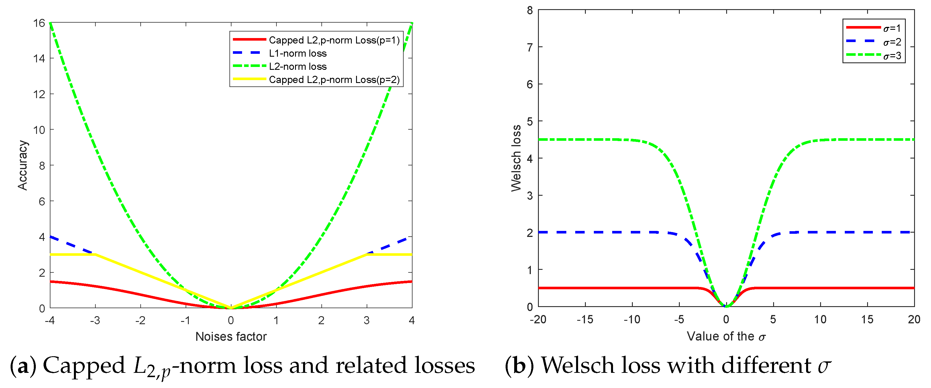
where the true value is given by y, $f\left(x\right)$ is the predicted value and $\sigma$ is the adjustable parameters. As shown in Figure 1a, we change the parameter C value from 1 to 3, and we can see that the upper bound of Welsch is gradually increasing and slowly converging. Observation (18), when $y-f\left(x\right)$ approaches infinity, the upper bound of $L(y-f(x\left)\right)$ is $\frac{{\sigma }^2}{2}$, which means that the outliers in the model can be limited by Welsch loss.

2.4. RTELM

TELM is a very excellent and powerful classification model with a wide range of research and applications in various academic fields. But it uses the square $L_2$-norm and the hinge loss function, and the effect of outliers is usually exaggerated. From this, we cannot guarantee the robustness of the TSVM. Therefore, based on this basis, RTELM is proposed, which replaces the $L_2$-norm distance metric and the hinge loss function with the capped $L_1$-norm distance metric and the adaptive capped $L_{\theta \epsilon }$-norm loss function. The expression for the RTELM is given below:   

$$\begin{array}{cc}\hfill & \underset{{\beta }_1}{min}{\Sigma }_{i=1}^{m_1}min\left(\right|{\beta }_{1}h\left(x_i\right)|,{\epsilon }_1)+C_1{\Sigma }_{i=1}^{m_2}min(\frac{(1+\theta ){\xi }_{1,i}^2}{|{\xi }_{1,i}|+\theta },{\epsilon }_2)\hfill \\ \hfill & s.t-H_2{\beta }_1+{\xi }_1\ge e_2\hfill \end{array}$$

(19)

$$\begin{array}{cc}\hfill & \underset{{\beta }_2}{min}{\Sigma }_{i=1}^{m_2}min\left(\right|{\beta }_{2}h\left(x_i\right)|,{\epsilon }_3)+C_2{\Sigma }_{i=1}^{m_1}min(\frac{(1+\theta ){\xi }_{2,i}^2}{|{\xi }_{2,i}|+\theta },{\epsilon }_4)\hfill \\ \hfill & s.t{H}_1{\beta }_2+{\xi }_2\ge e_1\hfill \end{array}$$

(20)

where $C_1,C_2>0$ are regularization parameters, $e_1\in R^{m_1}$ and $e_2\in R^{m_2}$ are vectors of ones, and ${\epsilon }_1$, ${\epsilon }_2$, ${\epsilon }_3$ and ${\epsilon }_4$ are thresholding parameters. To solve the above optimization problems (14) and (15) more efficiently, we can reformulate the problems as the following approximation problems through the reweighted method [32]:

$$\begin{array}{cc}\hfill & \underset{{\beta }_1}{min}\frac{1}{2}{\left(H_1{\beta }_1\right)}^{T}Q{H}_1{\beta }_1+\frac{1}{2}{C}_1{\xi }_1^{T}U{\xi }_1\hfill \\ \hfill & s.t-H_2{\beta }_1+{\xi }_1\ge e_2\hfill \end{array}$$

(21)

$$\begin{array}{cc}\hfill & \underset{{\beta }_2}{min}\frac{1}{2}{\left(H_2{\beta }_2\right)}^{T}Q{H}_2{\beta }_2+\frac{1}{2}{C}_2{\xi }_2^{T}Z{\xi }_2\hfill \\ \hfill & s.t-H_1{\beta }_2+{\xi }_2\ge e_1\hfill \end{array}$$

(22)

where $e_2\in R^{m_2}$ and $e_1\in R^{m_1}$ are vectors of ones, Q, G, U and Z are four diagonal matrices with i-th diagonal elements as

$$q_i=\left\{\begin{array}{l}\frac{1}{|{\beta }_1·h\left(x_i\right)|},|{\beta }_1·h\left(x_i\right)|\le {\epsilon }_1\hfill \\ smallval,otherwise.\hfill \end{array}\right.$$

(23)

$$g_i=\left\{\begin{array}{l}\frac{1}{|{\beta }_2·h\left(x_i\right)|},|{\beta }_2·h\left(x_i\right)|\le {\epsilon }_3\hfill \\ smallval,otherwise.\hfill \end{array}\right.$$

(24)

$$u_i=\left\{\begin{array}{l}(1+\theta )\frac{|{\xi }_{1,i}|+2\theta }{2\left(\right|{\xi }_{1,i}{|+\theta )}^2},\frac{(1+\theta ){\xi }_{1,i}^2}{|{\xi }_{1,i}|+\theta }\le {\epsilon }_2\hfill \\ smallval,otherwise.\hfill \end{array}\right.$$

(25)

$$z_i=\left\{\begin{array}{c}(1+\theta )\frac{|{\xi }_{2,i}|+2\theta }{2\left(\right|{\xi }_{2,i}{|+\theta )}^2},\frac{(1+\theta ){\xi }_{2,i}^2}{|{\xi }_{2,i}|+\theta }\le {\epsilon }_4\hfill \\ smallval,otherwise.\hfill \end{array}\right.$$

(26)

According to the optimization theory and the dual theory, the Wolfes dual problems of (16) and (17) are obtained as follows:

$$\underset{\alpha \ge 0}{min}\frac{1}{2}{\alpha }^T(H_2{\left(H_1^{T}Q{H}_1\right)}^{-1}{H}_2^T+\frac{1}{C_1}{U}^{-1})\alpha -e_2^T\alpha$$

(27)

Similarly,

$$\underset{\vartheta \ge 0}{min}\frac{1}{2}{\vartheta }^T(H_1{\left(H_2^{T}Q{H}_2\right)}^{-1}{H}_1^T+\frac{1}{C_2}{Z}^{-1})\alpha -e_1^T\vartheta$$

(28)

where $\alpha$, $\vartheta$ are the Lagrange multipliers.

2.5. Capped $L_{2,p}$-Norm

In TELM and other related areas, the $L_2$-norm is often applied in building the model, but $L_2$-norm is differentiable, and the negative effects of outliers may be magnified. ${\parallel .\parallel }_2^p$ is mainly used to enhance the robustness of the model by making fall within the interval of $(0,2]$ [32,33]. Therefore, we build different models for different problems by choosing the parameter $0<p\le 2$, which makes the $L_{2,p}$-norm more robust. For any vector $\alpha \in R^n$ and parameters $0<p\le 2$, $L_{2,p}$-norm and capped $L_{2,p}$-norm are defined as

$$\begin{array}{c}\hfill f_1\left(\alpha \right)={\left({\Sigma }_{i=1}^n{\alpha }_{i^n}\right)}_2^p\end{array}$$

(29)

$$\begin{array}{c}\hfill f_2\left(\alpha \right)=min({\left({\Sigma }_{i=1}^n{\alpha }_{i^n}\right)}_2^p,\epsilon )\end{array}$$

(30)

where $\epsilon \ge 0$ is the threshold parameter. From the above analysis and Figure 1, the robustness of capped $L_{2,p}$-norm is stronger than capped $L_1$-norm and capped $L_2$-norm, which is a generalization and extension of capped $L_1$-norm and capped $L_2$-norm.

More details can refer to [30].

3. Main Contribution

In this section, we place the Welsch loss and $L_{2,p}$-norm into the model TELM and obtain the two proposed models, CWTELM and FCWTELM. At the same time, to test the stability of the above models, we conducted a convergence analysis of them.

3.1. CWTELM

The primary problem of the model we built can be written as

$$\begin{array}{cc}\hfill & \underset{{\beta }_1}{min}\sum _{i=1}^{m_1}min(\parallel {\beta }_1{h}_{x_i}{\parallel }_2^p,{\epsilon }_1)+C_1\sum _{i=1}^{m_2}[1-exp(-\frac{{{\xi }_{1,i}}^2}{2{\sigma }^2})],\hfill \\ \hfill & s.t-H_2{\beta }_1+{\xi }_1\ge e_2.\hfill \end{array}$$

(31)

$$\begin{array}{cc}\hfill & \underset{{\beta }_2}{min}\sum _{i=1}^{m_2}min(\parallel {\beta }_2{h}_{x_i}{\parallel }_2^p,{\epsilon }_2)+C_2\sum _{i=1}^{m_1}[1-exp(-\frac{{{\xi }_{1,i}}^2}{2{\sigma }^2})],\hfill \\ \hfill & s.t-H_1{\beta }_2+{\xi }_2\ge e_1.\hfill \end{array}$$

(32)

where $C_1\ge 0$ and $C_2\ge 0$, $e_1\in R^{m_1}$ and $e_2\in R^{m_2}$ are the unit vectors.

To address the above issues, we let

$$\left\{\begin{array}{c}{R}_1\left({\beta }_1\right)=\sum _{i=1}^{m_1}min(\parallel {\beta }_1{h}_{x_i}{\parallel }_2^p,{\epsilon }_1)\hfill \\ L_1\left({\beta }_1\right)=C_1\sum _{i=1}^{m_2}[1-exp(-\frac{{\xi }_{1,i}^2}{2{\sigma }^2})]\hfill \end{array}\right.$$

(33)

Further, we let

$$\begin{array}{c}\hfill maxL\left({\beta }_1\right)=C_1\sum _{i=1}^{m_2}exp(-\frac{{\xi }_{1,i}^2}{2{\sigma }^2})=I\left({\beta }_1\right)\end{array}$$

(34)

Similarly,

$$\begin{array}{c}\hfill maxL\left({\beta }_2\right)=C_2\sum _{i=1}^{m_2}exp(-\frac{{\xi }_{2,i}^2}{2{\sigma }^2})=I\left({\beta }_2\right)\end{array}$$

(35)

Thus, (31) and (32) can be written as

$$\left\{\begin{array}{c}\underset{{\beta }_1}{max}I\left({\beta }_1\right)-R\left({\beta }_1\right)\hfill \\ \underset{{\beta }_2}{max}I\left({\beta }_2\right)-R\left({\beta }_2\right)\hfill \end{array}\right.$$

(36)

For an easier computation, we define a function $g\left(v\right)=-vlog(-v)+v,v_i<0,v=(v_1,v_2,\dots ,v_m)$, based on the theory of conjugate functions, we have   

$$\begin{array}{c}\hfill I\left({\beta }_1\right)=\underset{V<0}{sup}[c_1\sum _{i=1}^{m_1}(v_i\frac{{\xi }_{1,i}^2}{2{\sigma }^2}-g\left(v_i\right)]\end{array}$$

(37)

where $v_i=-exp(-\frac{{\xi }_{1,i}^2}{2{\sigma }^2})$.

Then,

$$\begin{array}{c}\hfill \underset{{\beta }_1,v<0}{max}M({\beta }_1,v)=c_1\sum _{i=1}^{m_1}(v_i\frac{{\xi }_{1,i}^2}{2{\sigma }^2}-g\left(v_i\right))-R\left({\beta }_1\right)\end{array}$$

(38)

Thus, the following formula holds true:

$$\begin{array}{cc}\hfill & \underset{{\beta }_1}{min}{\Sigma }_{i=1}^{m_1}min(\parallel {\beta }_{1}h\left(x_i\right){\parallel }_2^p,{\epsilon }_1)+\frac{c_1}{2{\sigma }^2}{\xi }_{1,\mathrm{i}}\Omega {\xi }_{1,i}\hfill \\ \hfill & s.t-H_2{\beta }_1+{\xi }_1\ge e_2\hfill \end{array}$$

(39)

$$\begin{array}{cc}\hfill & \underset{{\beta }_2}{min}{\Sigma }_{i=1}^{m_2}min(\parallel {\beta }_{2}h\left(x_i\right){\parallel }_2^p,{\epsilon }_2)+\frac{c_2}{2{\sigma }^2}{\xi }_{2,\mathrm{i}}\Omega {\xi }_{2,i}\hfill \\ \hfill & s.t{H}_1{\beta }_2+{\xi }_2\ge e_1\hfill \end{array}.$$

(40)

In order to optimize the objective function smoothly, we will introduce concave duality in Theorem 1.

Theorem 1.

Let $g\left(\theta \right)$: $Rn\to R$ is a continuous non-convex function, suppose $h\left(\theta \right):Rn\to \Omega \subset Rn$ is a map with range Ω. We assume that a concave function $\overline{g}\left(u\right)$ defined on Ω exists, such that $g\left(\theta \right)=g\left(h\right(\theta \left)\right)$ holds. Therefore, the non-convex function $g\left(\theta \right)$ can be expressed as [30]

$$\begin{array}{c}\hfill g\left(\theta \right)=\underset{v\in R^n}{inf}[V^{T}h\left(\theta \right)-g^{*\left(v\right)}]\end{array}$$

(41)

According to the convex dual theorem, the convex dual of $g\left(\theta \right):R\to R$ is written as

$$\begin{array}{c}\hfill g^{*}\left(v\right)=\underset{u\in }{inf}[V^{T}h\left(\theta \right)-g^{*\left(v\right)}]\end{array}$$

(42)

Moreover, the minimum value on the right side of formula (28) is

$$\begin{array}{c}\hfill v^{*}=\frac{\alpha \overline{g\left(\theta \right)}}{\alpha \theta }{|}_{u=h\left(\theta \right)}\end{array}$$

(43)

Proof. 

Thus, based on Theorem 1, we give a convex function $g\left(\theta \right):R\to R$, that makes arbitrary $\theta >0$

$$\begin{array}{c}\overline{g}\left(\theta \right)=min({\theta }^{\frac{p}{2}},\epsilon )\hfill \end{array}$$

(44)

Assuming $h\left(\mu \right)={\mu }^2$, we can find that

$$\begin{array}{c}min(\parallel \beta h\left(x_i\right){\parallel }_2^p,\epsilon )=\overline{g}\left(h\left(\mu \right)\right)\hfill \end{array}$$

(45)

where $\mu =\parallel \beta h\left(x_i\right){\parallel }_2$.

Therefore, based on (39), (40) and (45) can be written as

$$\begin{array}{cc}\hfill & \underset{{\beta }_1}{min}{\Sigma }_{i=1}^{m_1}\overline{g}\parallel {\beta }_{1}h\left(x_i\right){\parallel }_2^2+\frac{C_1}{2{\sigma }^2}{\xi }_{1,i}^T\Omega {\xi }_{1,i}\hfill \\ \hfill & s.t-H_2·{\beta }_1+{\xi }_1\ge e_2\hfill \end{array}$$

(46)

$$\begin{array}{cc}\hfill & \underset{{\beta }_2}{min}{\Sigma }_{i=1}^{m_1}\overline{g}\parallel {\beta }_{2}h\left(x_i\right){\parallel }_2^2+\frac{C_2}{2{\sigma }^2}{\xi }_{2,i}^T\Omega {\xi }_{2,i}\hfill \\ \hfill & s.t{H}_1·{\beta }_2+{\xi }_2\ge e_1\hfill \end{array}$$

(47)

Let ${\theta }_1=h\left({\mu }_1\right)={\parallel {\beta }_{1}h\left(x_i\right)\parallel }_2^2$, by Theorem 1, and the first term of (46) can be expressed as

$$\begin{array}{c}\hfill min(\parallel {\beta }_{1}h\left(x_i\right){\parallel }_2^p,{\epsilon }_1)=\overline{g}(\parallel {\beta }_{1}h\left(x_i\right){\parallel }_2^2)=\underset{f_{ii}\ge 0}{inf}{f}_{ii}h\left({\mu }_1\right)-g^{*}\left(f_{ii}\right)\end{array}$$

(48)

Here, the concave dual function of $g\left({\theta }_1\right)$ is

$$g^{*}\left(f_{ii}\right)=\underset{{\theta }_1}{inf}[f_{ii}-\overline{g}\left({\theta }_1\right)]=\underset{{\theta }_1}{inf}\left\{\begin{array}{c}{f}_{ii}{\theta }_1-{{\theta }_1}^{\frac{p}{2}},{\theta }_1^{\frac{2}{p-2}}<{\epsilon }_1\hfill \\ f_{ii}{\theta }_1-{\epsilon }_1,{\theta }_1^{\frac{p}{2}}\ge {\epsilon }_1\hfill \end{array}\right.$$

(49)

After the optimization of ${\theta }_1$ in Equation (49), we have

$$g^{*}\left(f_{ii}\right)=\left\{\begin{array}{c}{f}_{ii}{\left(\frac{2}{p}{f}_{ii}\right)}^{\frac{2}{p-2}}-{\left(\frac{2}{p}{f}_{ii}\right)}^{\frac{2}{p-2}},{\theta }_1^{\frac{2}{p-2}}<{\epsilon }_1\hfill \\ f_{ii}{\epsilon }_1^{\frac{2}{p}}-{\epsilon }_1,{\theta }_1^{\frac{p}{2}}\ge {\epsilon }_1\hfill \end{array}\right.$$

(50)

Therefore, the objective function (39) can be further written as

$$\begin{array}{cc}\hfill & \underset{{\beta }_1}{min}{\Sigma }_{i=1}^{m_1}min(\parallel {\beta }_{1}h\left(x_i\right){\parallel }_p^2),{\epsilon }_1)+\frac{C_1}{2{\sigma }^2}{\xi }_{1,i}^T\Omega {\xi }_{1,i}\hfill \\ \hfill ⟺& \underset{{\beta }_1}{min}{\Sigma }_{i=1}^{m_1}\underset{f_{ii}\ge 0}{inf}{L}_i({\beta }_1,f_{ii},{\epsilon }_1)+\frac{C_1}{2{\sigma }^2}{\xi }_{1,i}^T\Omega {\xi }_{1,i}\hfill \\ \hfill ⟺& \underset{({\beta }_1,f_{ii}\ge 0)}{min}{\Sigma }_{i=1}^{m_1}{L}_i({\beta }_1,f_{ii},{\epsilon }_1)+\frac{C_1}{2{\sigma }^2}{\xi }_{1,i}^T\Omega {\xi }_{1,i}\hfill \end{array}$$

(51)

where

$$L_i({\beta }_1,f_{ii},{\epsilon }_1)=\left\{\begin{array}{c}{f}_{ii}{\theta }_1-f_{ii}{\left(\frac{2}{p}{f}_{ii}\right)}^{\frac{2}{p-2}}+{\left(\frac{2}{p}{f}_{ii}\right)}^{\frac{2}{p-2}},{\theta }_1^{\frac{p}{2}}<{\epsilon }_1.\hfill \\ f_{ii}{\theta }_1-f_{ii}{\epsilon }_1^{\frac{2}{p}}+{\epsilon }_1,{\theta }_1^{\frac{p}{2}}\ge {\epsilon }_1.\hfill \end{array}\right.$$

(52)

Similarly, let ${\theta }_2=h\left({\mu }_2\right)={\parallel {\beta }_{2}h\left(x_i\right)\parallel }_2^2$, $g^{*}\left(k_{ii}\right)$ is expressed as a concave dual function of $\overline{g}\left({\theta }_2\right)$, so, formula (40) can be written as

$$\begin{array}{cc}\hfill & \underset{{\beta }_2}{min}{\Sigma }_{i=1}^{m_1}min(\parallel {\beta }_2{\parallel }_p^2,{\epsilon }_3)+\frac{C_2}{2{\sigma }^2}{\xi }_{2,i}^T\Omega {\xi }_{2,i}\hfill \\ \hfill ⟺& \underset{{\beta }_2}{min}{\Sigma }_{i=1}^{m_1}\underset{k_{ii}\ge 0}{inf}{L}_i({\beta }_2,k_{ii},{\epsilon }_3)+\frac{C_2}{2{\sigma }^2}{\xi }_{2,i}^T\Omega {\xi }_{2,i}\hfill \\ \hfill ⟺& \underset{{\beta }_2,f_{ii}\ge 0}{min}{\Sigma }_{i=1}^{m_2}{L}_i({\beta }_2,k_{ii},{\epsilon }_3)+\frac{C_2}{2{\sigma }^2}{\xi }_{2,i}^T\Omega {\xi }_{2,i}\hfill \end{array}$$

(53)

where

$$L_i({\beta }_2,k_{ii},{\epsilon }_3)=\left\{\begin{array}{c}{k}_{ii}{\theta }_2-k_{ii}{\left(\frac{2}{p}{f}_{ii}\right)}^{\frac{2}{p-2}}+{\left(\frac{2}{p}{k}_{ii}\right)}^{\frac{2}{p-2}},{\theta }_2^{\frac{p}{2}}<{\epsilon }_3.\hfill \\ k_{ii}{\theta }_2-k_{ii}{\epsilon }_1^{\frac{2}{p}}+{\epsilon }_2,{\theta }_2^{\frac{p}{2}}\ge {\epsilon }_3.\hfill \end{array}\right.$$

(54)

The objective functions (52) and (54) solve the optimization algorithm by alternately learning the optimal classifiers. We calculated the gradient of the function $g\left(\theta \right)$ with respect to $\theta$ as follows:

$$\frac{\partial \overline{g}\left(\theta \right)}{\partial \theta }=\left\{\begin{array}{c}\frac{p}{2}{\theta }^{\frac{p}{2}-1},0<\theta <{\epsilon }^{\frac{2}{p}}\hfill \\ 0,\theta >{\epsilon }^{\frac{2}{p}}\hfill \end{array}\right.$$

(55)

If ${\theta }_1=h\left({\mu }_1\right)={\parallel {\beta }_{1}h\left(x_i\right)\parallel }_2^2$, we can obtain

$$\begin{array}{c}\hfill f_{ii}=\frac{\partial \overline{g}\left(\theta \right)}{\partial \theta }{\mid }_{{\theta }_1}={\parallel {\beta }_{1}h\left(x_i\right)\parallel }_2^2=\left\{\begin{array}{c}\frac{p}{2}\parallel {\beta }_{1}h\left(x_i\right){\parallel }_2^2,0<{\parallel {\beta }_{1}h\left(x_i\right)\parallel }_2^2<{\epsilon }_1\hfill \\ 0,else\hfill \end{array}\right.\end{array}$$

(56)

Likewise, if ${\theta }_2=h\left({\mu }_2\right)={\parallel {\beta }_{2}h\left(x_i\right)\parallel }_2^2$, we can obtain

$$\begin{array}{c}\hfill k_{ii}=\frac{\partial \overline{g}\left({\theta }_2\right)}{\partial {\theta }_2}{\mid }_{{\theta }_2}={\parallel {\beta }_{2}h\left(x_i\right)\parallel }_2^2=\left\{\begin{array}{c}\frac{p}{2}\parallel {\beta }_{2}h\left(x_i\right){\parallel }_2^2,0<{\parallel {\beta }_{2}h\left(x_i\right)\parallel }_2^2<{\epsilon }_3\hfill \\ 0,else.\hfill \end{array}\right.\end{array}$$

(57)

□

It is important that to understand the relationship between parameters more clearly, we set the distance from sample $x_i$ to the hyperplane as X. If $X>{\epsilon }_1$, then $f_{ii}$ is almost 0, then the sample $x_i$ is considered an outlier and discarded. Additionally, $d_{ii}$ is similar to $f_{ii}$. When the variables $f_{ii}$ and $d_{ii}$ are fixed, to solve the classifier related parameters ${\beta }_1$ and ${\beta }_2$, the optimization problems (39) and (40) can be written as

$$\begin{array}{cc}\hfill & \underset{{\beta }_1}{min}{\Sigma }_{i=1}^{m_1}{f}_{\left(ii\right)}\parallel {\beta }_{1}h\left(x_i\right){\parallel }_2^2+\frac{C_1}{2{\sigma }^2}{\xi }_{1,i}^T\Omega {\xi }_{1,i}\hfill \\ \hfill & s.t-H_2·{\beta }_1+{\xi }_1\ge e_2\hfill \end{array}$$

(58)

$$\begin{array}{cc}\hfill & \underset{{\beta }_2}{min}{\Sigma }_{i=1}^{m_2}{k}_{\left(ii\right)}\parallel {\beta }_{2}h\left(x_i\right){\parallel }_2^2+\frac{C_2}{2{\sigma }^2}{\xi }_{2,i}^T\Omega {\xi }_{2,i}\hfill \\ \hfill & s.t{H}_1·{\beta }_2+{\xi }_2\ge e_1\hfill \end{array}$$

(59)

Let $F=diag(f_{11},f_{22},f_{33},\dots ,f_{m_1,m_1})$ be the $m_1$-diagonal matrix, and $K=diag(k_{11},k_{22},k_{33},$$\dots ,k_{m_2,m_2})$ be a diagonal matrix of $m_2$, so that (39) and (40) are equivalent to

$$\begin{array}{cc}\hfill & \underset{{\beta }_1}{min}{\left({\beta }_{1}h\left(x_i\right)\right)}^{T}F\left({\beta }_{1}h\left(x_i\right)\right)+\frac{C_1}{2{\sigma }^2}{\xi }_{1,i}^T\Omega {\xi }_{1,i}\hfill \\ \hfill & s.t-H_2·{\beta }_1+{\xi }_1\ge e_2\hfill \end{array}$$

(60)

$$\begin{array}{cc}\hfill & \underset{{\beta }_2}{min}{\left({\beta }_{2}h\left(x_i\right)\right)}^{T}K\left({\beta }_{2}h\left(x_i\right)\right)+\frac{C_2}{2{\sigma }^2}{\xi }_{2,i}^T\Omega {\xi }_{2,i}\hfill \\ \hfill & s.t{H}_1·{\beta }_2+{\xi }_2\ge e_1\hfill \end{array}$$

(61)

The corresponding Lagrange function of the above optimization problem (60) can be rewritten as

$$L({\beta }_1,{\xi }_1)=\frac{1}{2}{\left({\beta }_{1}h\left(x_i\right)\right)}^{T}F\left({\beta }_{1}h\left(x_i\right)\right)+\frac{1}{2{\sigma }^2}{C}_1{\xi }_1^T\Omega {\xi }_1-{\alpha }^T(-H_2{\beta }_1+{\xi }_1-e_2)$$

(62)

where $\alpha$ is a Lagrange multiplier. Differentiating the Lagrangian function with respect to ${\beta }_1$ and ${\beta }_2$ yields the following Karush–Kuhn–Tucker (KKT) conditions

$$\left\{\begin{array}{ccc}\frac{\partial L}{\partial \beta }=h\left(x_i\right)F\left({\beta }_{1}h\left(x_1\right)\right)+{\alpha }^T{H}_2=0,\hfill & \hfill \left(i\right)& \\ \frac{\partial L}{\partial \xi }={\sigma }^{\frac{1}{2}}{C}_2\Omega {\xi }_1+{\alpha }^T=0,\hfill & \hfill \left(ii\right)& \\ {\alpha }^T(-H_2{\beta }_1+{\xi }_1-e_2)=0,\hfill & \hfill \left(iii\right)& \\ \alpha \ge 0.\hfill & \hfill \left(iv\right)\end{array}\right.$$

(63)

By combining formulas (i) and (ii), we can obtain

$${\beta }_1=-{\left(H_1^{T}F{H}_1\right)}^{-1}\left(H_2^T\alpha \right)$$

(64)

Similarly, we can also obtain ${\xi }_1={(C_2\Omega )}^{-1}{\alpha }^T$, so the dual problem of (60) is

$$\underset{\alpha \ge 0}{min}\frac{1}{2}{\alpha }^T(H_2\left(H_1^{T}Q{H}_1\right)H_2^T+\frac{1}{C_1}{U}^{-1})\alpha -e_2^T\alpha$$

(65)

At the same time, the dual problem of (61) as follows:

$$\underset{\vartheta \ge 0}{min}\frac{1}{2}{\vartheta }^T(H_1\left(H_2^{T}G{H}_2\right)H_1^T+\frac{1}{C_2}{Z}^{-1})\vartheta -e_1^T\vartheta$$

(66)

where $\alpha$, $\vartheta$ is the Lagrange multiplier.

3.2. FCWTELM

Reduce the computation time complexity of CWTELM

$$\begin{array}{cc}\hfill & \underset{{\beta }_1}{min}\sum _{i=1}^{m_1}min(\parallel {\beta }_1·h_{x_i}{\parallel }_2^p,{\epsilon }_1)+C_1\sum _{i=1}^{m_2}[1-exp(-\frac{{{\xi }_{1,i}}^2}{2·{\sigma }^2})],\hfill \\ \hfill & s.t-H_2·{\beta }_1+{\xi }_1=e_2.\hfill \end{array}$$

(67)

$$\begin{array}{cc}\hfill & \underset{{\beta }_2}{min}\sum _{i=1}^{m_2}min(\parallel {\beta }_2·h_{x_i}{\parallel }_2^p,{\epsilon }_2)+C_2\sum _{i=1}^{m_1}[1-exp(-\frac{{{\xi }_{2,i}}^2}{2·{\sigma }^2})],\hfill \\ \hfill & s.t-H_1·{\beta }_2+{\xi }_2=e_1.\hfill \end{array}$$

(68)

Equivalent to processing the second item of FCWTELM, further, (67) and (68) written as

$$\begin{array}{cc}\hfill & \underset{{\beta }_1}{min}\sum _{i=1}^{m_1}min(\parallel {\beta }_1·h_{x_i}{\parallel }_2^p,{\epsilon }_1)+\frac{C_1}{2{\sigma }^2}{\xi }_{1,\mathrm{i}}\Omega {\xi }_{1,i},\hfill \\ \hfill & s.t-H_2·{\beta }_1+{\xi }_1=e_2.\hfill \end{array}$$

(69)

$$\begin{array}{cc}\hfill & \underset{{\beta }_2}{min}\sum _{i=1}^{m_2}min(\parallel {\beta }_2·h_{x_i}{\parallel }_2^p,{\epsilon }_2)+\frac{c_2}{2{\sigma }^2}{\xi }_{2,\mathrm{i}}\Omega {\xi }_{2,i},\hfill \\ \hfill & s.t-H_1·{\beta }_1+{\xi }_2=e_1.\hfill \end{array}$$

(70)

Replace the equality constraint into the objective function, we obtain

$$\underset{{\beta }_1}{min}\sum _{i=1}^{m_1}min(\parallel {\beta }_1·h_{x_i}{\parallel }_2^p,{\epsilon }_1)+C_1{\Omega }_1{\parallel e_2+H_2{\beta }_1\parallel }_2^2$$

(71)

$$\underset{{\beta }_2}{min}\sum _{i=1}^{m_1}min(\parallel {\beta }_2·h_{x_i}{\parallel }_2^p,{\epsilon }_2)+C_2{\Omega }_2{\parallel e_1-H_1{\beta }_2\parallel }_2^2$$

(72)

Further, similar to the handling of CWTELM, we can obtain

$$\begin{array}{cc}\hfill & \underset{{\beta }_1}{min}{\left({\beta }_{1}h\left(x_i\right)\right)}^{T}F\left({\beta }_{1}h\left(x_i\right)\right)+\frac{C_1}{2{\sigma }^2}{\xi }_{1,i}^T\Omega {\xi }_{1,i}\hfill \end{array}$$

(73)

$$\begin{array}{cc}\hfill & \underset{{\beta }_2}{min}{\left({\beta }_{2}h\left(x_i\right)\right)}^{T}K\left({\beta }_{2}h\left(x_i\right)\right)+\frac{C_2}{2{\sigma }^2}{\xi }_{2,i}^T\Omega {\xi }_{2,i}\hfill \end{array}$$

(74)

The (73) differential for ${\beta }_1$ to zero gives

$$2H^{T}DH{\beta }_1+C_1{H}_2^T\Omega e_2+c_1{H}_2^T{\Omega }_1{H}_1{\beta }_1=0$$

(75)

So,

$${\beta }_1=-{(2H_1^{T}FH+C_1{\Omega }_1{H}_2^T{H}_2)}^{-1}{C}_1{H}_2^T{\Omega }_1{e}_2$$

(76)

Similarly,

$${\beta }_1={(2H_2^{T}F{H}_2+C_2{H}_1^T{\Omega }_2{H}_1)}^{-1}{C}_2{H}_1^T{\Omega }_2{e}_1$$

(77)

3.3. Convergence Analysis

Lemma 1.

For any scalar t, when $0<p\le 2$, inequality ${2\left|t\right|}^p-p{t}^2+p-2\le 0$ is always established.

Lemma 2.

For arbitrary $x\ne y\in R^n$, if $f\left(x\right)=x-\frac{x^2}{2y}$, then inequality $f\left(x\right)<f\left(y\right)$ is always established.

Lemma 3.

For any non-zero vector α, β, when $0<p\le 2$, inequality

$${\parallel \alpha \parallel }_2^p-\frac{p}{2}{\parallel \beta \parallel }_2^{p-2}{\parallel \alpha \parallel }_2^2\le {\parallel \beta \parallel }_2^p-\frac{p}{2}{\parallel \beta \parallel }_2^{p-2}{\parallel \beta \parallel }_2^2$$

(78)

is always established.

Theorem 2.

Algorithm 1 will monotonously reduce the objective of problems (49) and (50), respectively, in each iteration.

Algorithm 1 Training CWTELM.

Input: Training data: Training set $T_1={\left\{x_i,y_i\right\}}_l^{i=1}$, $i=1,\dots ,l$, where $x_i\in R^n$, $x_j\in R^n$, $y_i\in \left\{-1,+1\right\}$; activation function $G\left(x\right)$, and the number of hidden node number L, the parameters $C_1$, $C_2$, ${\epsilon }_1$, ${\epsilon }_2$, ${\epsilon }_3$, ${\epsilon }_4$, ${\delta }_1$ and ${\delta }_2$.

${\beta }_1^{*}$ and ${\beta }_2^{*}$;

Process:

1. Initialize $F\in {\mathbb{R}}^{m_1\times m_1}$ and $Q\in {\mathbb{R}}^{m_2\times m_2}$;$K\in {\mathbb{R}}^{m_2\times m_2}$ and $U\in {\mathbb{R}}^{m_1\times m_1}$;

2. $\alpha$ and $\beta$;

3. Passing $Z_1=-{(H^{T}FH+C_{3}I)}^{-1}{E}^T\alpha$ and $Z_2={(E^{T}KE+C_{4}I)}^{-1}{H}^T\beta$ Calculate $Z_1$ and $Z_2$,

4. Accordingly, update matrix separately $Q,U,F,K$.

Proof. 

Let

$$J=\underset{{\beta }_1}{min}{\Sigma }_{i=1}^{m_1}min(\parallel {\beta }_{1}h\left(x_i\right){\parallel }_2^P),{\epsilon }_1)+c_1\sum _{i=1}^{m_2}min[1-exp(-\frac{{\left({\xi }_{1,i}\right)}^2}{2{\sigma }^2}),{\epsilon }_2]$$

(79)

When $\parallel {\beta }_{1}h\left(x_i\right)\parallel <{\epsilon }_1$ and $\parallel 1-exp(-\frac{{\left({\xi }_{1,i}\right)}^2}{2{\sigma }^2})\parallel <{\epsilon }_2$

$$J=\underset{\beta ,{\xi }_{1,i}}{min}{\Sigma }_{i=1}^{m_1}min(\parallel {\beta }_{1}h\left(x_i\right){\parallel }_2^P),{\epsilon }_1)+c_1\sum _{i=1}^{m_2}[1-exp(-\frac{{\left({\xi }_{1,i}\right)}^2}{2{\sigma }^2})]$$

(80)

Let $J=J_1+J_2$, where

$$J_1=\underset{\beta }{min}{\Sigma }_{i=1}^{m_1}{\parallel {\beta }_{1}h\left(x_i\right)\parallel }_2^P$$

(81)

$$J_2=c_{1}min\sum _{i=1}^{m_2}[1-exp(-\frac{{\left({\xi }_{1,i}\right)}^2}{2{\sigma }^2}),{\epsilon }_2]$$

(82)

For $J_1$, assuming that $Z^{k+1}$ is the solution of the $k+1$ iteration of Algorithm 1:

$${[\beta ,h\left(x_i\right)]}^{(k+1)}=min\frac{1}{2}{\left({\beta }_{1}h\left(x_i\right)\right)}^T{F}^k\left({\beta }_{1}h\left(x_i\right)\right)$$

(83)

Apparently, the Algorithm 1 has the following formula in iteration k,

$${\left[{\left({\beta }_{1}h\left(x_i\right)\right)}^{k+1}\right]}^T{F}^{\left(K\right)}[{\beta }_{1}h\left(x_i\right]\le {\left[{\left({\beta }_{1}h\left(x_i\right)\right)}^k\right]}^T{F}^{\left(K\right)}[{\beta }_{1}h\left(x_i\right]$$

(84)

Reduce to

$$\frac{P}{2}\parallel {\left({\beta }_{1}H\left(x_i\right)\right)}^{k+1}{\parallel }_2^2\parallel {\left({\beta }_{1}H\left(x_i\right)\right)}^{k+1}{\parallel }_{P-2}^2\le \frac{P}{2}\parallel {\left({\beta }_{1}H\left(x_i\right)\right)}^k{\parallel }_2^2{\parallel {\left({\beta }_{1}H\left(x_i\right)\right)}^k\parallel }_{P-2}^2$$

(85)

Based on Lemma 3, we obtain

$$\parallel {\beta }_{1}H{\left(x_i\right)}^{k+1}{\parallel }_2^p-\frac{P}{2}\parallel {\left({\beta }_{1}h\left(x_i\right)\right)}^k{\parallel }_2^{p-2}\parallel {\left({\beta }_{1}h\left(x_i\right)\right)}^{k+1}{\parallel }_2^2\le \parallel {\beta }_{1}H{\left(x_i\right)}^k{\parallel }_p^2-\frac{P}{2}\parallel {\left({\beta }_{1}h\left(x_i\right)\right)}^k{\parallel }_{p-2}^2{\parallel {\left({\beta }_{1}h\left(x_i\right)\right)}^k\parallel }_2^2$$

(86)

Combining (85) and (86), we have

$$\parallel {\beta }_{1}H{\left(x_i\right)}^{k+1}{\parallel }_2^p\le {\parallel {\beta }_{1}H{\left(x_i\right)}^k\parallel }_2^p$$

(87)

Thus, the $J_1$ is convergent. Next, we discuss the convergence of $g\left(v\right)=1-exp(-v^2)=1-exp(-\frac{{\xi }_{1,i}^2}{2{\sigma }^2})$, where $V=\frac{{\xi }_{1,i}^2}{\sqrt{2}\sigma }$, there exists a convex function $\psi \left(s\right)$, we have $g\left(v\right)={inf}_{s>0}\frac{1}{2}s{v}^2+\psi \left(s\right)$, and when V is fixed, we have the minimum $s^{*}$, which satisfies

$$g\left(v\right)=\underset{s>0}{inf}\frac{1}{2}s{v}^2+\psi \left(s\right)=\frac{1}{2}{s}^{*}{v}^2+\psi \left(s^{*}\right)$$

(88)

where $s^{*}=2exp(-v^2)$, so $L\left(h\left(x\right)\right)=c\lambda {inf}_{s>0}\left(\frac{s\left({\xi }_{1,i}^2\right)}{4{\sigma }^2}+\psi \left(s\right)\right)$.

The above formula is converted into

$$\begin{array}{c}\hfill \begin{array}{cc}& \underset{{\beta }_1}{min}{\Sigma }_{i=1}^{m_1}min(\parallel {\beta }_{1}h\left(x_i\right){\parallel }_2^P),{\epsilon }_1)+c\lambda {\Sigma }_{i=1}^N\underset{s_i>0}{inf}\left(\frac{s\left({\xi }_{1,i}^2\right)}{4{\sigma }^2}+\psi \left(s_i\right)\right)\hfill \\ & ⟺\underset{{\beta }_1}{min}{\Sigma }_{i=1}^{m_1}min(\parallel {\beta }_{1}h\left(x_i\right){\parallel }_2^P),{\epsilon }_1)+c\lambda {\Sigma }_{i=1}^N\left(\frac{s\left({\xi }_{1,i}^2\right)}{4{\sigma }^2}+\psi \left(s_i\right)\right)\hfill \end{array}\end{array}$$

(89)

The above problem is solved by alternating iterative algorithms. Specifically, in the k-th iteration, we bring $s\left(k\right)$ into problem (89):

$$\underset{\beta }{min}{\parallel \beta \parallel }_2^2+\sum _{i=1}^N{c}_i{\parallel {\xi }_{1,i}\parallel }_1$$

(90)

where $c_i=\frac{c\lambda {s_i}^{k-1}}{4{\sigma }^2}$ and $c_i>0$. By introducing the relaxation variable $\xi$ in Equation (90), the optimization problem becomes

$$\begin{array}{cc}\hfill & \underset{{\beta }_1,{\xi }_1}{min}{\parallel \beta \parallel }_2^2+\sum _{i=1}^N{c}_i{{\xi }_i}^2\hfill \\ \hfill & s.t{\xi }_{1,i}\ge 0,i=1,\dots ,N\hfill \end{array}$$

(91)

The optimal solution ${\beta }^{\left(k\right)}$ can be obtained by solving (85) and then putting it in (91).

$$\underset{s>0}{min}\sum _{i=1}^N\left(\frac{s_i\left({{\xi }_{1,i}}^2\right)}{4{\sigma }^2}+\psi \left(s_i\right)\right)$$

(92)

According to Theorem 1, we obtain the minimal solution

$${s_i}^{\left(k\right)}=2exp(-\frac{{\left({\xi }_{1,i}\right)}^2}{2{\sigma }^2}),i=1,\dots ,N$$

(93)

From (84), (85) and Lemma 2, we can obtain $A_1(\beta ,s)\ge A\left(\beta \right)\ge 0$, then the sequence is lower bounded. Assuming that $\beta \left(k\right)$ and $s\left(k\right)$ are obtained after k iterations, we use $s\left(k\right)$ to optimize the formula (93) on $\beta$:

$$A_1({\beta }^k,s^{\left(k\right)})\ge A_1({\beta }^{(k+1)},s^{\left(k\right)})$$

(94)

And $\beta (k+1)$ is optimized for formula (64) on s:

$$A_1({\beta }^{(k+1)},s^{\left(k\right)})\ge A_1({\beta }^{(k+1)},s^{(k+1)})$$

(95)

Concluding from the above inequality, we have □

$$A_1({\beta }^{\left(k\right)},s^{\left(k\right)})\ge A_1({\beta }^{(k+1)},s^{(k+1)})$$

(96)

Therefore, $J_2$ is convergence. Thus, the sequence is convergence.

4. Experimental

4.1. Experiments Setup

ELM has the goodness of rapid learning, strong approximation and excellent generalization, both in regression as well as multiple classification. To judge the performance of our proposed CWTELM and FCWTELM, we compare CWTELM and FCWTELM with other traditional methods systematically, including ELM, Correntropy-based Robust Extreme Learning Machine (CHELM), TELM, Capped $L_1$-norm Twin Support Vector Machine (CTSVM) and RTELM. For CTSVM, FCWTELM and CWTELM, we stop the iteration process when the target value of two consecutive iterations is less than 0.001 and the number of iterations is greater than 50. The parameters selected by all of the above algorithms are ${\epsilon }_1={\epsilon }_2={10}^{-4}$, $c,c_1,c_2,c_3,c_4:$$\left\{10i|-5,-4,\dots ,4,5\right\}$, $\sigma :\left\{10i|i=-4,-3,\dots ,3,4\right\}$, $\lambda :\left\{10i|i=-7,-6,-5,\dots ,5,6,7\right\}$, $k:\left\{3,7,9,11\right\}$, $\eta :\left\{0.001,0.005,0.01,0.05,0.1,0.5,1,1.5,2\right\}$ and L:$\left\{50,100,200,400,500,1000,2000\right\}$. We selected the optimal parameters for the parameters c, $c_1$, $c_2$, $\lambda$, $\sigma$, and Land by using 10-fold cross-validation and grid search. ELM, TELM, CHELM, RTELM, CTSVM, CWTELM and FCWTELM use the activation function $1/(1+exp(-(w·x+b)\left)\right)$ (w, bare random generation). Meanwhile, we measure the classification performance of all algorithms by the accuracy (ACC). Acc is expressed as [23]

$$\mathrm{ACC}=\frac{\mathrm{TP}+\mathrm{TN}}{\mathrm{TP}+\mathrm{TN}+\mathrm{FP}+\mathrm{FN}}$$

(97)

Specifically, TP indicates true positives, TN represents true negatives, FN expresses false negatives, and FP represents false positives. Furthermore, the computational efficiency of each algorithm is represented by learning time. All of the measures are conducted on the MATLAB 2021a and run on the system configuration 11th Gen Intel (R) Core (TM) i5-11357G7 processor (2.40 GHz) with 16 GB of memory.

4.2. Artificial Dataset

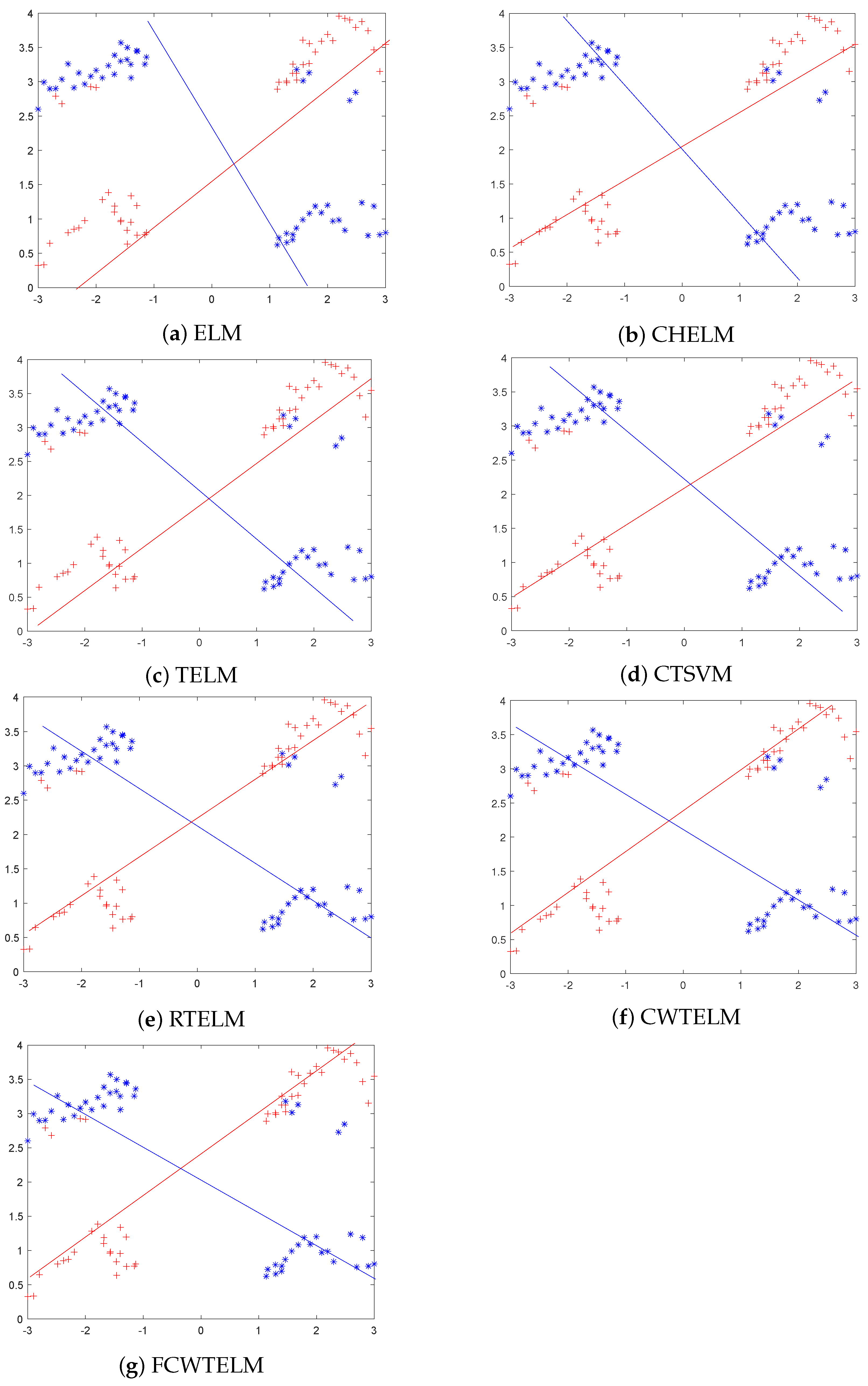
Since our proposed algorithm is mainly used to solve the binary classification problem, so to verify the effectiveness of FCWTELM and CWTELM, we generated a class of binary classification datasets based on Gaussian distribution. First, 100 artificial data samples are grouped into two classes, one positive and one negative. The positive class is expressed by +, and the other is represented by *. Since the outliers influence the classification performance of the model significantly, nine outliers were inserted to compare the robustness of ELM, CHELM, TELM, CTSVM, RTELM, CWTELM and FCWTELM. Then, the 9 outliers were divided into four positive and five negative, as shown in Figure 2.

4.3. UCI Dataset

The UCI (http://archive.ics.uci.edu/ml/datasets.html (accessed on 28 December 2022) dataset is one of the widely used standard datasets, and the UCI dataset can provide a relative standard basis, making the model comparison more objective. Since data acquisition and processing is a time-consuming and laborious task, in the case of limited time and resources, we applied eight datasets, which are: Australian, Balance, Vote, Cancer, Wholesale, QSAR, Pima, WDBC. As shown in

Table 3. Characteristics of UCI Datasets.

Datasets	Samples	Attributes	Datasets	Samples	Attributes
Australian	690	14	Cancer	699	9
Balance	576	4	Wholesale	440	7
Vote	432	16	WDBC	569	30
QSAR	1055	41	Pima	768	8

, they represent different data types and characteristics, such a selection also makes the study results more reliable. And we will follow up the experiment with our algorithms in more datasets. To verify the classification behavior of our two models, we conducted a series of experiments on the above datasets. In consideration of that noise is an important factor to measure the robustness of the algorithm, we will study these eight datasets of different noise rates, and if the classification accuracy varies smoothly for different noise rates, the algorithm shows good robustness.

4.4. Experimental Results on the UCI Datasets without Outliers

In this part, to test the classification behavior of the CWTELM, FCWTELM and other correlative algorithms, we ran eight UCI datasets on these algorithms. In

Table 4. Experimental results on UCI datasets with 0% Gaussian noise.

	ELM	CHELM	TELM	CTSVM	RTELM	CWTELM	FCWTELM
Datasets	ACC (%)	ACC (%)	ACC (%)	ACC (%)	ACC (%)	ACC (%)	ACC (%)
	Times (s)	Times (s)	Times (s)	Times (s)	Times (s)	Times (s)	Times (s)
Australian	85.74	86.53	86.69	84.93	86.58	$\mathbf{88.24}$	$\mathbf{86.70}$
	$\mathbf{1.541}$	4.561	2.093	3.466	5.125	6.847	$\mathbf{0.536}$
Balance	85.11	91.04	90.41	89.29	$\mathbf{94.64}$	$\mathbf{96.43}$	91.07
	$\mathbf{1.739}$	4.543	3.112	3.097	4.381	4.853	$\mathbf{0.427}$
Vote	94.58	95.60	95.48	95.58	$\mathbf{95.81}$	$\mathbf{97.62}$	92.65
	1.043	4.547	$\mathbf{0.901}$	9.310	6.234	4.654	$\mathbf{0.587}$
Cancer	80.61	86.43	86.33	86.88	90.75	$\mathbf{94.20}$	$\mathbf{91.30}$
	1.706	5.013	$\mathbf{0.873}$	2.771	4.274	6.256	$\mathbf{0.581}$
wholesale	75.07	74.31	74.56	73.49	81.40	$\mathbf{86.05}$	$\mathbf{81.44}$
	1.476	4.675	$\mathbf{0.937}$	2.819	3.948	4.123	$\mathbf{0.369}$
QSAR	84.43	81.66	86.87	$\mathbf{88.31}$	87.64	$\mathbf{88.46}$	87.50
	1.541	3.043	$\mathbf{0.629}$	7.856	7.798	11.437	$\mathbf{0.798}$
Pima	77.76	76.78	78.01	72.68	$\mathbf{78.86}$	$\mathbf{79.01}$	76.32
	2.674	3.622	$\mathbf{1.316}$	6.047	7.664	6.492	$\mathbf{0.772}$
WDBC	$\mathbf{95.85}$	95.32	95.55	95.13	95.21	$\mathbf{98.21}$	94.64
	1.435	8.951	$\mathbf{1.225}$	9.549	6.449	5.224	$\mathbf{0.454}$

, all the test outcomes are based on the optimal parameters. The time (s) represents the average running time obtained by each algorithm according to the optimal parameters, and the accuracy (ACC) represents the average classification accuracy. As can be seen from Table 4, from a classification point of view, CWTELM performs better than the other six algorithms on all the datasets. In many cases, ACC of the FCWTELM is in the forefront, and the average running time of the algorithm is shorter. By analyzing the test results in the above, we can reach the conclusion that using the $L_{2,p}$-norm in the TELM framework is able to promote the classification performance. Thus, the proposed CWTELM and FCWTELM are valid supervised algorithms without outliers.

4.5. Robustness against Outliers

See from the previous subsection that CWTELM and FCWTELM have good classification performance, to further test the robustness of them to the outliers, we considered three scenarios, respectively: the noise levels $M=0.1$, $M=0.2$ and $M=0.25$.

With noise levels of $M=0.1$, $M=0.2$ and $M=0.25$, all tests outcomes are revealed in

Table 5. Experimental results on UCI datasets with 10% Gaussian noise.

	ELM	CHELM	TELM	CTSVM	RTELM	CWTELM	FCWTELM
Datasets	ACC (%)	ACC (%)	ACC (%)	ACC (%)	ACC (%)	ACC (%)	ACC (%)
	Times (s)	Times (s)	Times (s)	Times (s)	Times (s)	Times (s)	Times (s)
Australian	79.83	80.21	81.03	80.45	81.98	$\mathbf{85.29}$	$\mathbf{82.35}$
	$\mathbf{1.523}$	4.631	2.143	3.487	5.187	6.473	$\mathbf{0.521}$
Balance	83.32	84.43	83.21	87.23	85.71	$\mathbf{91.07}$	$\mathbf{89.29}$
	$\mathbf{1.909}$	4.876	2.453	4.417	4.418	4.497	$\mathbf{0.426}$
Vote	93.57	92.22	94.65	95.01	$\mathbf{95.43}$	$\mathbf{95.24}$	91.35
	0.978	3.872	$\mathbf{0.376}$	9.654	5.503	4.717	$\mathbf{0.587}$
Cancer	79.36	83.46	85.48	85.36	84.06	$\mathbf{89.86}$	$\mathbf{86.96}$
	1.758	5.001	$\mathbf{0.773}$	2.608	4.316	6.354	$\mathbf{0.590}$
wholesale	74.47	75.31	73.56	73.14	76.64	$\mathbf{83.72}$	$\mathbf{78.37}$
	1.476	4.657	$\mathbf{0.879}$	2.892	4.063	4.150	$\mathbf{0.373}$
QSAR	73.61	72.43	79.64	78.79	84.31	$\mathbf{85.58}$	$\mathbf{84.62}$
	$\mathbf{1.931}$	6.778	2.789	9.852	10.754	11.198	$\mathbf{0.763}$
Pima	72.21	73.45	73.47	70.38	75.91	$\mathbf{76.32}$	$\mathbf{84.62}$
	2.013	3.023	$\mathbf{1.482}$	6.924	6.765	6.714	$\mathbf{0.768}$
WDBC	88.53	89.26	87.63	91.43	$\mathbf{92.31}$	$\mathbf{96.43}$	91.07
	1.238	7.693	$\mathbf{0.924}$	8.988	5.973	6.608	$\mathbf{0.667}$

,

Table 6. Experimental results on UCI datasets with 20% Gaussian noise.

	ELM	CHELM	TELM	CTSVM	RTELM	CWTELM	FCWTELM
Datasets	ACC (%)	ACC (%)	ACC (%)	ACC (%)	ACC (%)	ACC (%)	ACC (%)
	Times (s)	Times (s)	Times (s)	Times (s)	Times (s)	Times (s)	Times (s)
Australian	76.48	78.85	78.91	79.80	$\mathbf{81.12}$	$\mathbf{83.82}$	80.88
	1.586	6.683	$\mathbf{0.774}$	9.710	8.740	7.704	$\mathbf{0.583}$
Balance	79.11	81.39	82.01	84.91	82.14	$\mathbf{87.50}$	$\mathbf{85.71}$
	$\mathbf{1.679}$	5.460	2.489	3.345	4.392	4.871	$\mathbf{0.424}$
Vote	92.51	90.23	93.76	94.19	94.43	$\mathbf{95.24}$	$\mathbf{95.36}$
	0.990	3.856	$\mathbf{0.401}$	9.348	5.607	5.321	$\mathbf{0.506}$
Cancer	79.25	80.15	82.67	85.29	84.06	$\mathbf{86.96}$	$\mathbf{85.51}$
	1.739	5.203	$\mathbf{0.798}$	2.661	4.346	6.952	$\mathbf{0.411}$
wholesale	74.19	74.91	73.06	72.21	74.22	$\mathbf{81.40}$	$\mathbf{76.74}$
	1.330	4.857	$\mathbf{0.896}$	3.412	3.953	4.119	$\mathbf{0.374}$
QSAR	64.87	65.44	68.44	68.56	76.92	$\mathbf{83.65}$	$\mathbf{79.81}$
	$\mathbf{2.245}$	10.212	4.443	11.387	12.876	10.844	$\mathbf{0.809}$
Pima	65.87	65.80	66.32	71.75	$\mathbf{73.31}$	$\mathbf{73.68}$	71.50
	1.746	2.498	$\mathbf{1.090}$	7.095	5.198	6.329	$\mathbf{0.931}$
WDBC	84.76	85.37	82.08	82.75	85.56	$\mathbf{92.86}$	$\mathbf{89.29}$
	1.389	8.918	$\mathbf{1.124}$	9.330	6.499	5.235	$\mathbf{0.509}$

and

Table 7. Experimental results on UCI datasets with 25% Gaussian noise.

	ELM	CHELM	TELM	CTSVM	RTELM	CWTELM	FCWTELM
Datasets	ACC (%)	ACC (%)	ACC (%)	ACC (%)	ACC (%)	ACC (%)	ACC (%)
	Times (s)	Times (s)	Times (s)	Times (s)	Times (s)	Times (s)	Times (s)
Australian	66.79	69.85	65.66	74.65	$\mathbf{76.76}$	$\mathbf{83.82}$	76.47
	1.413	6.747	$\mathbf{1.406}$	9.552	7.895	7.842	$\mathbf{0.724}$
Balance	78.39	80.11	81.12	85.46	85.71	$\mathbf{87.50}$	$\mathbf{85.72}$
	$\mathbf{1.710}$	2.539	3.411	3.279	4.494	4.664	$\mathbf{0.453}$
Vote	93.82	92.23	91.10	93.18	93.64	$\mathbf{93.86}$	$\mathbf{93.98}$
	0.893	3.653	$\mathbf{0.664}$	9.118	7.235	5.321	$\mathbf{0.508}$
Cancer	79.25	80.36	81.32	84.86	81.16	$\mathbf{85.61}$	$\mathbf{84.97}$
	1.739	5.210	$\mathbf{0.799}$	2.503	4.332	6.863	$\mathbf{0.404}$
wholesale	74.00	74.01	73.06	70.35	72.09	$\mathbf{79.07}$	$\mathbf{74.42}$
	1.404	5.110	$\mathbf{0.789}$	3.020	4.066	4.173	$\mathbf{0.374}$
QSAR	63.72	67.69	65.77	73.65	70.01	$\mathbf{74.04}$	$\mathbf{75.00}$
	$\mathbf{0.441}$	10.357	4.499	9.336	12.876	11.357	$\mathbf{0.790}$
Pima	65.83	65.59	65.29	70.39	$\mathbf{70.66}$	$\mathbf{73.68}$	69.74
	1.746	2.202	$\mathbf{1.045}$	6.691	7.836	6.394	$\mathbf{0.860}$
WDBC	77.56	75.57	79.09	80.12	84.64	$\mathbf{85.71}$	$\mathbf{85.71}$
	$\mathbf{1.401}$	8.631	1.553	9.407	6.639	5.248	$\mathbf{0.435}$

, respectively. Table 5, Table 6 and Table 7 show the experimental results of the seven algorithms on the eight datasets with the $0.1$, $0.2$ and $0.25$ noise levels. It is obvious that the accuracy of seven algorithms decreases after the introduction of outliers. Yet, except for some cases, the accuracy of CWTELM is still better than the other six algorithms. In many illustrations, the classification accuracy of FCWTELM is in the forefront of the seven algorithms, and its running time is the shortest among the other algorithms.

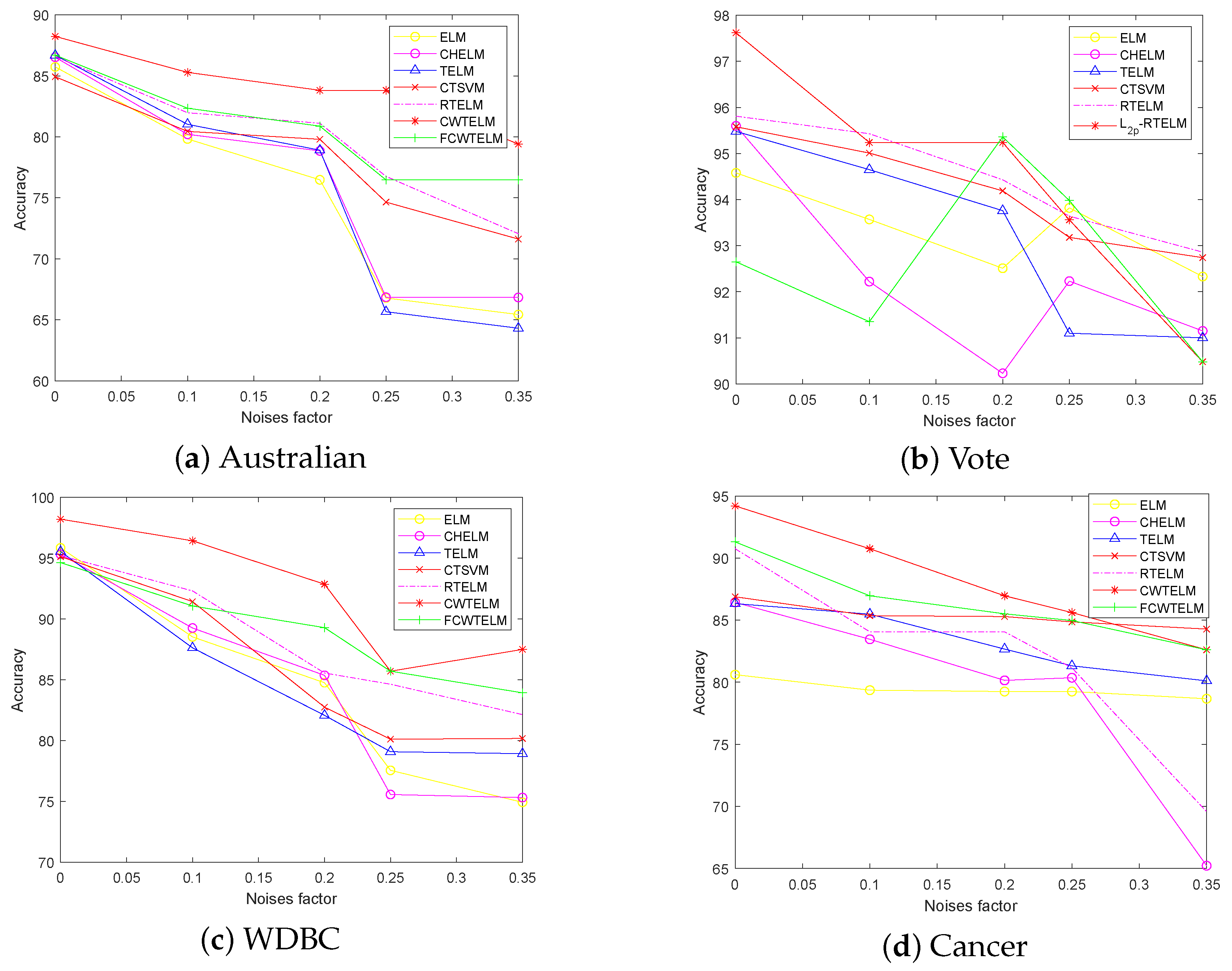
We take Vote, WDBC, Cancer, and Australia this four UCI datasets for examples and draw the line diagram of above seven algorithms under different Gaussian noise rates, which is shown in Figure 3. We can more intuitive to find that the accuracy of CWTELM and FCWTELM change more smoothly than the other five algorithms when the noise increases. Summarize the above experimental results, we can obtain the following conclusion: in the case of noise, CWTELM and FCWTELM still maintain the advantages of classification performance and robustness. In addition, the classification performance of CWTELM and FCWTELM is little different. Next we will use statistical monitoring analysis to further verify the accuracy of them.

4.6. Experimental Results on Artificial Dataset with Outliers

By tests on eight UCI datasets, we confirm that CWTELM and FCWTELM have better properties in classification and robustness. Therefore, to further explore the advantages of both algorithms, we will again validate their accuracy in the artificial dataset. The results are shown in Figure 4. Observing Figure 4, we find that the precision of the above seven frameworks classified varied in the order of containing outliers, from low to high, with roughly the same operation on UCI. The classification accuracy of the above seven models in the artificial dataset is, respectively, ELM 61.3%, CHELM 65.6%, TELM 67.0%, CTSVM 78%, RTELM 80%, CWTELM 84%, and FCWTELM 86%. It also further determined that the $L_{2,P}$-norm measure and the Welsch loss have significant positive effects on robustness and classification performance.

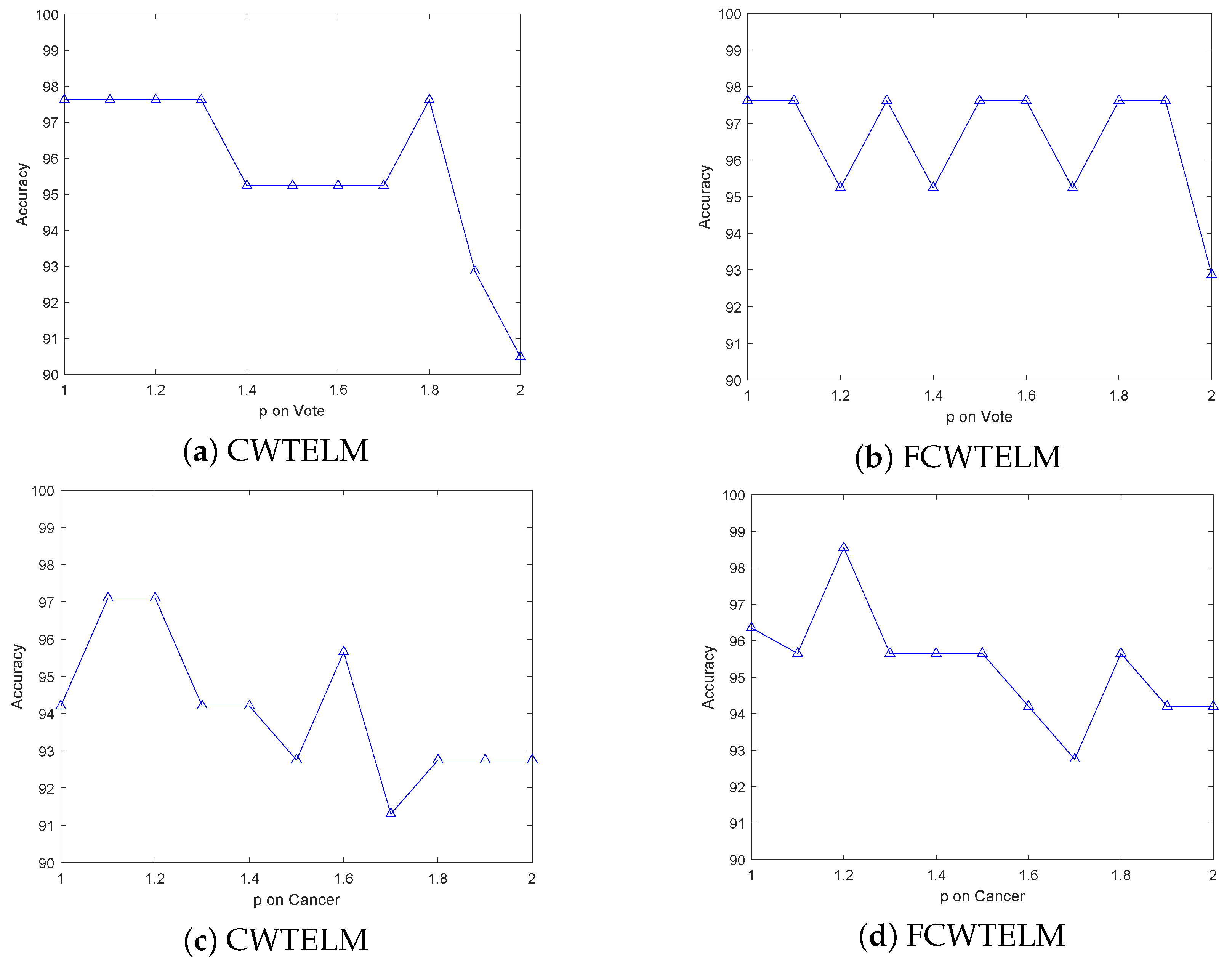
To verify the effect of parameter p on the models performance, we present the parameter analysis results in Figure 5. It can be seen from the Figure 5 that the proposed method is less affected by the parameters. In addition, we experiment on the accuracy of CWTELM and FCWTELM for different values of p. In Figure 5, we can find that many better accuracies are not achieved at p = 1 and p = 2, so it is a wise choice to introduce the $L_{2,p}$ norm metric.

4.7. Statistical Analysis

Within this segment, the Friedman test [34] is applied to analyze the significant differences among above algorithms across eight UCI datasets. The Friedman test was used to compare differences in paired groups across multiple related groups in a sample. Its null hypothesis is that there is no difference between groups, where the median observed values are equal across all groups. If the observed difference between groups is significant, the null hypothesis can be rejected and concluded that at least one group is significantly different. When the null hypothesis is rejected, we can perform a Nemenyi test [34]. The Nemenyi test is a post hoc test method that used to determine whether significant differences exist between multiple independent groups. It is based on a cross-consideration of the direction and variability of group differences to determine which groups differ significantly by comparing double comparisons between two groups. Then, we calculated the average accuracy and ranking of seven algorithms on 8 datasets, which is revealed in

Table 8. Average accuracy and ranking of the seven algorithms on the UCI datasets with different noise proportions.

	ELM	CHELM	TELM	CTSVM	RTELM	CWTELM	FCWTELM
Avg.ACC 10%	80.61	81.35	82.33	82.72	84.54	87.94	86.08
Avg.rank 10%	6.000	5.500	4.875	4.625	3.000	1.250	2.750
Avg.ACC 20%	77.13	77.77	78.41	79.93	81.47	85.64	83.10
Avg.rank 20%	6.000	5.750	5.000	4.500	2.625	1.375	2.750
Avg.ACC 25%	74.92	75.68	75.30	79.08	79.33	82.91	80.75
Avg.rank 25%	5.625	5.500	5.750	4.125	3.625	1.375	2.000

. First, taking a 20% Gaussian noise as an example, we can use the following formula to calculate the Friedman statistical variables:

$$X_F^2=\frac{12N}{k(k+1)}[\sum _j{R}_j^2-\frac{{k(k+1)}^2}{4}]=32.21$$

(98)

where N and k represent the number of UCI datasets and algorithms, as well as $R_j$ is the average rank of the j-th algorithm on the dataset used. In this paper, $k=7$ as well as $N=8$. Moreover, based on the $x_F^2$-distribution with $(k-1)$ degrees of freedom, we can obtain

$$F_F=\frac{(N-1)X_F^2}{N(k-1)-X_F^2}=14.277$$

(99)

where $F_F(k-1)$, $(k-1)(N-1)$ follows the f distribution, with $(k-1)$ and $(k-1)(N-1)$ degrees of freedom. Furthermore, for $\alpha =0.05$, we can obtain an $F_{\alpha }=(6,42)=2.324$. Clearly, $F_F>F_{\alpha }$, and therefore we can reject the null hypothesis. From Table 8, we can see that the average ranking of CWTELM and FCWTELM is much lower than the other algorithms, meaning that our CWTELM and FCWTELM are more effective than the other algorithms. In addition, we further compared seven algorithms by the Nemenyi post hoc test method. When the average rank difference between the two algorithms is less than the cut-off value, the difference in performance between the two algorithms is not significant, or otherwise significant. By dividing the study range statistic by 2, we can obtain $q_{\alpha }=0.05=2.949$. Therefore, we calculate the critical difference value (CD) using the following formula:

$$CD=q_{\alpha }=0.1\sqrt{\frac{k(k+1)}{6N}}=2.949\times \sqrt{\frac{7(7+1)}{6\times 10}}=2.5858$$

(100)

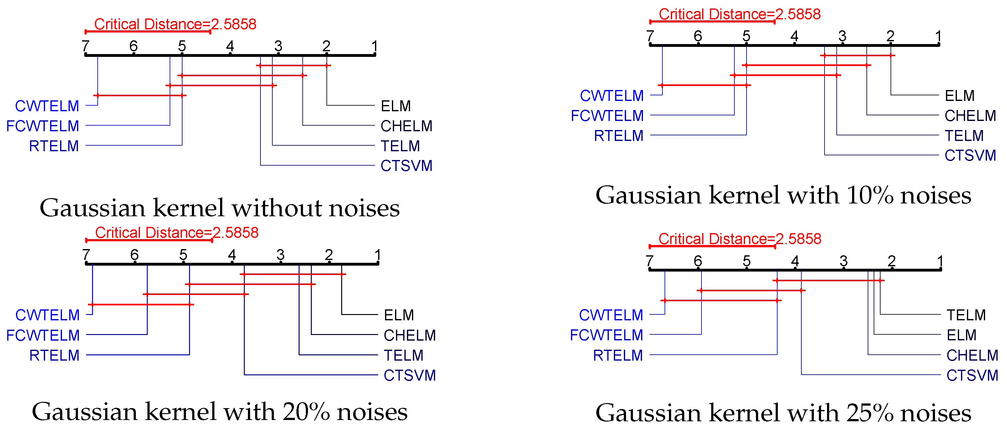
As shown in Figure 6, CWTELM and FCWTELM behave significantly better than ELM, CHELM, TELM, CTSVM and RTELM in classification. It can further be seen that there is no significant difference between CWTELM and FCWTELM, as the difference is smaller than the CD value. Therefore, it can be confirmed that the proposed methods CWTELM and FCWTELM have better performance by statistical analysis.

5. Conclusions

The Welsch loss function has good qualities such as smooth, non-convex and boundness and, therefore, it is more robust than the commonly used $L_1$ and $L_2$ losses. Capped $L_{2,p}$-norm is an excellent norm distance that can reduce the negative effects of outliers and thus improve the robustness of the model. In this paper, we proposed a distance metric optimization-driven robust twin extreme learning machine learning framework, namely CWTELM, which introduced Welsch loss and $L_{2,p}$-norm distance to the TELM in order to enhance the performance of robust. Then, to speed up the computation of CWTELM while maintaining its advantages, we presented a least square version of CWTELM, namely Fast CWTELM (FCWTELM). Meanwhile, we design two efficient iterative algorithms to solve CWTELM and FCWTELM, respectively, and guarantee their convergence and computational complexity in theory. To evaluate the performance of CWTELM and FCWTELM, we experiment with them with five classical algorithms in different datasets and different noise rates. In the absence of noise, CWTELM achieved the best results in seven datasets. The experimental results of FCWTELM in the eight datasets are slightly lower than CWTELM, but the gap is small, and its running time is the shortest among the seven algorithms. In the case of noise, we take 10% noise as an example, CWTELM achieved the best results in Australian, Balance, Cancer, Wholesale, QSAR, WDBC, and FCWTELM performed the best in Pima. From a running time perspective, FCWTELM has the fastest running speed in the six datasets and all within 1 s. In addition, we found that CWTELM and FCWTELM have little difference between no noise and 10% noise conditions in same dataset. We continue to observe the experimental data with 20% and 25% noise and can also obtain the above conclusions. To this end, this paper takes Australian, Vote, WDBC, and Cancer as examples to more clearly show the accuracy of the seven algorithms in the form of different noise proportions. Similarly, we also conducted comparative experiments on the seven algorithms in the artificial dataset, and showed the classification effect of the seven algorithms more intuitively in the form of a scatter plot. The performance of CWTELM and FCWTELM is still excellent. Finally, we carried out statistical tests on seven algorithms and verified that CWTELM and FCWTELM exceeded other five models and that the two models had no significant difference in performance. From the above works, we can obtain that CWTELM and FCWTELM alleviate the negative effects of outliers to some extent, so they have good robustness. Besides they also have little difference in classification performance and have a outstanding operation while maintaining the advantages of TELM. The algorithms CWTELM and FCWTELM proposed in this paper can be applied to pattern classification. On the one hand, our algorithm has good classification representation and robustness, and it can learn the nonlinear relationship between the input data. In this way, a high-precision classification model can be obtained. Therefore, our model is able to obtain more accurate results when performing the pattern classification. On the other hand, our algorithm can improve the robustness of pattern classification. They can automatically choose and solve the specificity in the classification process, and can deal with the noise between different categories, so they are more suitable for different pattern classification tasks in practical application scenarios. Of course, in addition to pattern classification, CWTELM and FCWTELM can also be applied in many fields, such as data mining, pattern recognition, action recognition in robot control, path planning, image classification and so on. In the future, to improve the algorithms we proposed, in-depth studying for them is necessary, such as exploring better loss functions for the TELM framework to improve the robustness of the model and algorithm performance. In addition, we can also deepen the basic research, derive the upper bound of their generalization ability, etc.

References

1. Guang-Bin, H.; Zhu, Q.; Siew, C. Extreme learning machine: Theory and applica tions. Neurocomputing 2006, 70, 489–501. [Google Scholar]
2. Huang, G.-B.; Chen, Y.; Babri, H.A. Classification ability of single hidden layer feedforward neural networks. IEEE Trans. Neural Netw. 2000, 11, 799–801. [Google Scholar] [CrossRef] [Green Version]
3. Han, K.; Yu, D.; Tashev, I. Speech emotion recognition using deep neural network and extreme learning machine. In Proceedings of the Interspeech 2014, Singapore, 14–18 September 2014. [Google Scholar]
4. Romanuke, V. Setting the hidden layer neuron number in feedforward neural network for an image recognition problem under Gaussian noise of distortion. Comput. Inf. Sci. 2013, 6, 38. [Google Scholar] [CrossRef] [Green Version]
5. Tiwari, S.; Bharadwaj, A.; Gupta, S. Stock price prediction using data analytics. In Proceedings of the 2017 International Conference on Advances in Computing, Communication and Control (ICAC3), Mumbai, India, 1–2 December 2017. [Google Scholar]
6. Imran, M.; Khan, M.R.; Abraham, A. An ensemble of neural networks for weather forecasting. Neural Comput. Appl. 2004, 13, 112–122. [Google Scholar]
7. Guang-Bin, H.; Zhu, Q.; Siew, C. Extreme learning machine: A new learning scheme of feedforward neural networks. In Proceedings of the IEEE International Joint Conference on Neural Networks, Budapest, Hungary, 25–29 July 2004. [Google Scholar]
8. Son, Y.J.; Kim, H.G.; Kim, E.H.; Choi, S.; Lee, S.K. Application of support vector machine for prediction of medication adherence in heart failure patients. Healthc. Inform. Res. 2010, 16, 253–259. [Google Scholar] [CrossRef]
9. Wang, G.; Zhao, Y.; Wang, D. A protein secondary structure prediction framework based on the extreme learning machine. Neurocomputing 2008, 72, 262–268. [Google Scholar] [CrossRef]
10. Yuan, L.; Soh, Y.C.; Huang, G. Extreme learning machine based bacterial protein subcellular localization prediction. In Proceedings of the 2008 IEEE International Joint Conference on Neural Networks (IEEE World Congress on Computational Intelligence), Hong Kong, China, 1–8 June 2008. [Google Scholar]
11. Abdul Adeel, M.; Minhas, R.; Wu, Q.M.J.; Sid-Ahmed, M.A. Human face recognition based on multidimensional PCA and extreme learning machine. Pattern Recognit. 2011, 44, 2588–2597. [Google Scholar]
12. Nizar, A.H.; Dong, Z.Y.; Wang, Y. Power utility nontechnical loss analysis with extreme learning machine method. IEEE Trans. Power Syst. 2008, 23, 946–955. [Google Scholar] [CrossRef]
13. Decherchi, S.; Gastaldo, P.; Dahiya, R.S.; Valle, M.; Zunino, R. Tactile-data classification of contact materials using computational intelligence. IEEE Trans. Robot. 2011, 27, 635–639. [Google Scholar] [CrossRef]
14. Choudhary, R.; Shukla, S. Reduced-Kernel Weighted Extreme Learning Machine Using Universum Data in Feature Space (RKWELM-UFS) to Handle Binary Class Imbalanced Dataset Classification. Symmetry 2022, 14, 379. [Google Scholar] [CrossRef]
15. Owolabi, T.O.; Abd Rahman, M.A. Prediction of Band Gap Energy of Doped Graphitic Carbon Nitride Using Genetic Algorithm-Based Support Vector Regression and Extreme Learning Machine. Symmetry 2021, 13, 411. [Google Scholar] [CrossRef]
16. Jayadeva; Khemchandani, R.; Chandra, S. Twin support vector machines for pattern classification. IEEE Trans. Pattern Anal. Mach. Intell. 2007, 29, 905–910. [Google Scholar] [CrossRef] [PubMed]
17. Hou, Q.; Zhang, J.; Liu, L.; Wang, Y.; Jing, L. Discriminative information-based nonparallel support vector machine. Signal Process. 2019, 162, 169–179. [Google Scholar] [CrossRef]
18. Nasiri, J.A.; Charkari, N.M.; Mozafari, K. Energy-based model of least squares twin support vector machines for human action recognition. Signal Process. 2014, 104, 248–257. [Google Scholar] [CrossRef]
19. Ghorai, S.; Mukherjee, A.; Dutta, P.K. Nonparallel plane proximal classifier. Signal Process. 2009, 89, 510–522. [Google Scholar] [CrossRef]
20. Wan, Y.; Song, S.; Huang, G.; Li, S. Twin extreme learning machines for pattern classification. Neurocomputing 2017, 260, 235–244. [Google Scholar] [CrossRef]
21. Reshma, R.; Bharti, A. Least squares twin extreme learning machine for pattern classification. In Innovations in Infrastructure: Proceedings of ICIIF 2018; Springer: Singapore, 2019. [Google Scholar]
22. Yuan, C.; Yang, L. Robust twin extreme learning machines with correntropy-based metric. Knowl.-Based Syst. 2021, 214, 106707. [Google Scholar] [CrossRef]
23. Ma, J.; Yang, L. Robust supervised and semi-supervised twin extreme learning machines for pattern classification. Signal Process. 2021, 180, 107861. [Google Scholar] [CrossRef]
24. Ma, J.; Yuan, C. Adaptive Safe Semi-Supervised Extreme Machine Learning. IEEE Access 2019, 7, 76176–76184. [Google Scholar] [CrossRef]
25. Shen, J.; Ma, J. Sparse Twin Extreme Learning Machine With ε -Insensitive Zone Pinball Loss. IEEE Access 2019, 7, 112067–112078. [Google Scholar] [CrossRef]
26. Zhang, K.; Luo, M. Outlier-robust extreme learning machine for regression problems. Neurocomputing 2015, 151, 1519–1527. [Google Scholar] [CrossRef]
27. Ke, J.; Gong, C.; Liu, T.; Zhao, L.; Yang, J.; Tao, D. Laplacian Welsch Regularization for Robust Semisupervised Learning. IEEE Trans. Cybern. 2020, 52, 164–177. [Google Scholar] [CrossRef]
28. Tokgoz, E.; Trafalis, T.B. Mixed convexity optimization of the SVM QP problem for nonlinear polynomial kernel maps. In Proceedings of the 5th WSEAS International Conference on Computers, Puerto Morelos, Mexico, 29–31 January 2011. [Google Scholar]
29. Xu, Z.; Lai, J.; Zhou, J.; Chen, H.; Huang, H.; Li, Z. Image Deblurring Using a Robust Loss Function. Circuits Syst. Signal Process. 2021, 41, 1704–1734. [Google Scholar] [CrossRef]
30. Wang, H.; Yu, G.; Ma, J. Capped L2,p-Norm Metric Based on Robust Twin Support Vector Machine with Welsch Loss. Symmetry 2023, 15, 1076. [Google Scholar] [CrossRef]
31. Ma, X.; Ye, Q.; Yan, H. L2,p-norm distance twin support vector machine. IEEE Access 2017, 5, 23473–23483. [Google Scholar] [CrossRef]
32. Li, C.-N.; Shao, Y.-H.; Deng, N.-Y. Robust L1-norm non-parallel proximal support vector machine. Optimization 2014, 65, 169–183. [Google Scholar] [CrossRef]
33. Yuan, C.; Yang, L. Capped L2,p-norm metric based robust least squares twin support vector machine for pattern classification. Neural Netw. 2021, 142, 457–478. [Google Scholar] [CrossRef]
34. Chapelle, O.; Scholkopf, B.; Zien, A. Semi-supervised learning (chapelle, o. et al., eds.; 2006) [book reviews]. IEEE Trans. Neural Netw. 2009, 20, 542. [Google Scholar] [CrossRef]
Figure 1. Loss Functions.
Axioms 12 00765 g001
Figure 2. Distribution of artificial datasets with outliers.
Axioms 12 00765 g002
Figure 3. Accuracies of five algorithms via different noises factors.
Axioms 12 00765 g003
Figure 4. The classification results on the artificial datasets.
Axioms 12 00765 g004
Figure 5. Accuracies of CWTELM and FCWTELM via different parameter p.
Axioms 12 00765 g005
Figure 6. Visualization of post-hoc tests for UCI datesets.
Axioms 12 00765 g006