Article

Model-Free Sliding Mode Enhanced Proportional, Integral, and Derivative (SMPID) Control

School of Engineering, University of the West of England, Frenchy Campus, Coldharbour Lane, Bristol BS16 1QY, UK
Axioms 2023, 12(8), 721; https://doi.org/10.3390/axioms12080721
Submission received: 27 June 2023 / Revised: 18 July 2023 / Accepted: 19 July 2023 / Published: 25 July 2023
(This article belongs to the Special Issue Advances in Analysis and Control of Systems with Uncertainties II)

Abstract

:
This study proposes a type of Sliding Mode-based Proportional, Integral, and Derivative (SMPID) controllers to establish a model-free (treat dynamic plants as a whole uncertainty) sliding model control (MFSMC) platform for Bounded-Input and Bounded-Output (BIBO) dynamic systems. The SMPID design (1) proposes a sliding mode error (rather than error) as the PID input, (2) directly links to Lyapunov asymptotic stability to provide total robust nonlinear dynamic inversion (NDI), and (3) reduces the chattering effects in terms of Lyapunov definite positive stability. Further, the study proposes a general SMC framework to accommodate asymptotic time stabilisation and finite-time stabilisation for both model-based and model-free designs. A U-control framework is presented to integrate the SMPID control (for NDI) and an invariant control (IC) (for specifying the whole control system’s dynamic and static responses), which significantly relaxes the PID tunings and generates the specified performance. To provide assurance and guidance for applications and expansions, this study presents the relevant fundamental analyses and transparent simulated bench tests. It should be noted that the new SMPID in forms of u = S M P I D ( σ ( e ) ) = P I D ( sliding - mode ) is different from that studied u = sliding - mode ( PID ( e ) ) in expression and functionality.

1. Introduction

A PID controller has been widely applied in almost all engineering (man-made) operational systems involving controls of motion and/or process [1,2]. The PID controller is mathematically defined by an integro-differential equation [3].
u ( t ) = P I D ( e ( t ) ) : u ( t ) = k p e ( t ) + k i 0 t e ( τ ) d τ + k d d e ( t ) d t
where u ( t ) is the PID output at time t , k p ,   k i , and k d are the tuning parameters for the proportional gain, the integral gain ( τ is the variable for the integration), and the derivative gain, respectively, e ( t ) is the PID input taken from the difference between the reference point and the measured system output in a closed-loop control system.
Figure 1 is presented below for quickly grasping the new PID/Figure 1c (with the author’s best knowledge, this is the first study) in comparison with the other PIDs.
This section takes a critical review of the closely related representative publications to justify its motivation, why we need this work, and what the major novelty/contributions are for academic research and industrial applications.
Formation of PID: The advantages of classical PID are widely witnessed, including its comparative simplicity, suitability for a wide range of industrial processes and motion control, and the availability of tuning rules for both mode-based and model-free designs. It is noted that the matured PID method is still theoretically studied for uncertain nonlinear systems, as reported in a top control journal publication [4]. There have been various modified PIDs proposed to provide extra functionalities, such as model-free intelligent PID (iPID) [5,6], in which the model-free control is structured with some classical functional analysis and elementary differential algebra. One of the merits of iPID is that it reduces the strange industrial ubiquity of classic PIDs and the great difficulty of tuning the PID gains in complex situations. It is noted that although it is named as model-free control, the iPID still takes simple model estimation online. A natural expansion of PIDs is nonlinear PIDs, either assigning nonlinear gains associated with PID variables [7] or functioning both gains and PID variables nonlinearly [8]. Conventional topics have received little attention in the last decade. The other notable variations of PID include self-tuning linear/nonlinear PID [9,10]; neural PID [11]; and fuzzy PID [12,13]. In summary, regarding the difference in PID formation, they have further functionalized the three terms (P, I, and D) in one way or another. A commonality of the PIDs in formation is that all the PID inputs are setup as the error e ( t ) , the difference between the reference point and the measured output. This has made it difficult to link the PID designs to Lyapunov stability, particularly when the PIDs are designed for the control of nonlinear plants. Therefore, if there is a novelty in assigning alternative PID input to increase PID functionality and effectiveness, a series of new comprehensive understandings/analyses should be followed up to support such new PID designs. This is the first novelty the study is trying to explore.
PID (gain) tuning: The PID tuning techniques have been widely studied from classical to modern optimisation rules [2,14]. There are various classical tuning methods—trial-and-error-based, for example, the famous Ziegler-Nichols step response method [3]. It has been observed that these classical tuning methods generally assume the types of plants (with or without integrator) and the shapes of outputs (monotonic or oscillatory), and then try, possibly iteratively, by simulations and/or real experiments in either an open loop or a closed loop, to obtain some numerical and graphical features of the controlled system responses to determine the PID gains. These methods are simple and straightforward without using advanced control theory or understanding. However, these tunings do not guarantee always giving the desired dynamic and static responses, particularly in the control of nonlinear dynamic plants. These methods should be encouraged in the initial control system tuning before considering the other advanced, normally complicated tuning methods. Regarding the optimisation tuning rules [2,15], representatively these include model-free optimisation [16], eagle perching optimisation with PID tuning potential [17], neural network and fuzzy logic enhanced tunings [12,18], and Self-tuning/auto-tuning [9,19]. In summary, all the approaches have laid a solid foundation for PID tuning progression, even though the optimisation of three PID gains (parameters) is a time-consuming task no matter whether model-based or model-free optimisations are used. In critical analysis, PID tuning, the dilemma of choosing PID gains from multiple choices, and the significant difficulty of specifying dynamic response have been critical issues with almost all the exiting model-free PIDs. There is a possibility to improve the shortcomings mentioned, i.e., to relieve the PID control role of only stabilisation rather than demanding both stabilisation and dynamic response. Consequently, the PID gain tuning is largely relaxed, which requires determining the PID controller output with some new insights and criteria. This is the second novelty the study is trying to explore.
Sliding mode PID: Regarding the integration of SMC and PID, there are two streams. The first one has had certain popularity and takes the sliding mode PID in forms of u = sliding - mode ( PID ( e ) ) , such as active disturbance rejection with sliding mode control for course/path following of underactuated ships [20] and variations [21,22,23]. This type of PID is used to replace conventional sliding mode functions with PID and uses the error between the reference and the output as the PID input. The majority of such controls with PID sliding surfaces [24] still request the plant model to determine the equivalent control; therefore, robustness is relatively weaker than those approaches that take the whole plant model as uncertainty. It has been noted that recent milestone work has been devoted to the design of a proportional integral derivative-like continuous sliding mode controller (PID-CSMC) [25] with finite-time sliding mode from the route of continuous sliding mode controllers (CSMC) and super twisting control [26]. It has been observed that most of these CSMC do not have any criteria for selecting the PID gains from such sets [25]. The milestone work has clearly provided a way for selecting such gains using an uncertainty upper bound-related parameter in design. This is in a mode-free configuration. The second aspect that needs to be improved with the SMPID design is to ensure accurate dynamic response (such as that specified by damping ratio and undamped natural frequency) from stabilisation. The other recently studied SMPID stream takes the form of u = S M P I D ( σ ( e ) ) = P I D ( sliding - mode ) in terms of model-free and asymptotic stability [27,28], which have intuitively taken proportional (P) control to determine the equivalent control but are not generally considered such prototypes of SMPID control and beyond. This is the third novelty the study is trying to explore. In comparison of the two types of sliding mode PIDs, it should be noted that the PID-CSMC can only provide 2nd-order sliding mode functions due to the PID formation, while the SMPID can provide high-order sliding mode functions because it takes the same formation as that of conventional SMC. Accordingly, SMPID keeps the merits of conventional SMC and enhances conventional SMC by taking in the PID function.
U-model based control (U-control): This is a generalised control system design platform with two feedback loops [29,30], by which (1) robust plant dynamic inversion is used to cancel both plant nonlinearity and dynamics simultaneously in the inner loop, which consequently results in a unit constant/identity matrix, and (2) an outer loop is separately configured with a linear controller to achieve the specified control system performance. The approach to dealing with nonlinear dynamic inversion (NDI) is the key to U-control. Such type of research has gone through (1) model-matched [31], (2) model-mismatched [32,33], and (3) model-free [28]. The current research tendency is to apply U-control to facilitate/simplify the other conventional control system design approaches, particularly in dealing with nonlinear dynamics and model uncertainties. A perception of the U-control is that it provides seamless supplementary support to almost all the conventional control design methods because all of these involve dynamic inversion in one way or another. In brief, U-control has been developing along the route from problem complexity to solution simplicity and generality. This study is a good showcase for integrating PID with SMC and linear control (damping ratio and undamped natural frequency) to enhance the control system design’s effectiveness and efficiency.
From the analyses above, there is potential to upgrade SMPID in terms of formation and functionality. This study considers the following two aspects.
(a)
Take u = S M P I D ( σ ( e ) ) = P I D ( sliding - mode ) to form a new SMPID to satisfy the Lyapunov asymptotic stability condition σ 2 0 σ ˙ σ 0 rather than σ 2 0 σ ˙ σ = 0 (conventionally used for solving nominal models to determine the equivalent control). Note that the condition σ ˙ σ = 0 is one of the causes of the chattering effect (because chattering is subject to such stability).
(b)
Significantly reduce the difficulty in tuning PID gains due to the high demands on the PID control roles; that is, a well-designed PID control has been widely demanded for both dynamic and static response. A properly designed PID could just be used for the plant’s dynamic inversion and then leave the dynamic specifications (e.g., damping ratio and undamped natural frequency) to the other controller within a generalised U-control system framework. Consequently, the PID gain tuning is significantly relaxed to achieve the pre-specified dynamic/static performance.
Accordingly, the major contributions of the study are outlined below.
(1)
Propose a sliding mode function σ = σ ( x ˜ , t ) as the PID controller input, The replacement of conventional PID input makes the input take in comprehensive state error to form a sliding model function in terms of the Hurwitz polynomial n and the derivative of the sliding mode σ ˙ is assigned with another polynomial σ ˙ = u = ρ ( σ ) to determine the PID controller output satisfying the asymptotic stability condition σ ˙ σ 0 rather than the conventional stability condition σ ˙ σ = 0 (NB, this is not asymptotic stability and one of the courses of chattering). The new SMPID effectively drives the system states x to achieve σ = σ ( x ˜ , t ) = 0 and keep on reaching them. The plant is treated as a whole uncertainty.
(2)
The new SMPID u = S M P I D ( σ ( e ) ) = P I D ( sliding - mode ) is different from the other types of SMPID u = sliding - mode ( PID ( e ( t ) ) . In terms of practical applications, the new controller can be more easily implemented with commercial PID instruments.
(3)
Generalisation of SMC formation: A section is contributed to propose a generalised SMC design prototype to cover both asymptotic time stabilisation and finite-time stabilisation for both model-based and model-free designs. The SMPID is one of the implementations.
(4)
Significantly reduce the PID tuning effort in practise: Multiple choices of PID parameters (gains) Distinctively, this new method only needs the PID gains satisfying Lyapunov asymptotic stability conditions to achieve dynamic inversion in the inner loop; the exact linear dynamic and static responses (for example ω n 2 s 2 + 2 ζ ω n s + ω n 2 ) are specified/achieved in the outer loop within the U-control framework. In other words, the new PID parameter tuning is largely relaxed, as it is only for stability. However, almost all the other tuning methods (Ziegler-Nichols trial and error methods, model-free online optimisations, etc.) are not only demanding for stability but more demanding for dynamic (transient) responses, which cannot be uniquely specified with a group of PID gains.
(5)
Significantly reduce the chattering effect: It is noted that σ ˙ = 0 is used for determining the equivalent control in conventional model-based SMC. This is one of the roots of chattering because σ ˙ = 0 gives σ ˙ σ = 0 (stable but not asymptotically stable, and chattering is subject to such stability). The new approach determines the equivalent control with σ ˙ σ 0 (asymptotic stability), this also gives a relaxed sliding band thickness setup without losing accuracy, which relieves the struggling trade-off between accuracy and chattering. This has very practical significance for saving operational energy costs and reducing hardware wear and tear. The simulated case studies well demonstrate the claims.
(6)
As the independent/separate design of dynamic inversion and whole control system performance controller within the U-control system framework, this study provides a potential for co-design for practical applications, such as Unmanned Aerial Vehicles (UAV), separating the airframe design and its control system design, then seamlessly integrating them to simplify/speed up the whole system setup and maintenance. The principle/technique should be applicable to most motion and processing systems.
(7)
Provide a set of transparent, user-friendly simulation demonstrations for guiding applications and expansions.
The remaining study includes four sections. Section 2 presents preliminaries for the reference conducting the following development. Section 3 presents various SMPID-based model-free controllers, including a monotone-bounded hyperbolic tangent (tanh) function-based nonlinear SMPID to remove the need for switching control in SMC systems, and analyses the associated properties to provide assurance for expansions and applications. Section 3.5 proposes a generalised SMC structure to accommodate both asymptotic time stabilisation and finite-time stabilisation for both model-based and model-free designs. Section 4 presents a U-control-based comprehensive computational experimental platform to demonstrate the analytical results and validate the control system configuration of the function block connections. Two bench test examples are provided to illustrate and compare the simulated control system operations. Section 5 summarises the study with the major outcomes and potential expansions.

2. Preliminary

2.1. Problem Formulation—Control of Model Unknown Nonlinear Dynamic Plants

The plant: Consider a class of general single input, single output (SISO) nth-order nonlinear dynamic plants, described by
P : y ( n ) = f y ( 0 n 1 ) , u , d
where the triplets { y , u , d } are the plant output, input, and external disturbance, respectively, and y ( 0 n 1 ) = y y ( n 1 ) T n is the n 1 order output derivative vector. It should be noted that model (2) can be expressed in state space equations as well by letting x = y ( 0 n 1 ) = x 1 = y x 2 = y ˙ x n 1 = y ( n 1 ) T n and x n = f x , u , d .
Assumption 1. 
f : u y , an unknown mapping from the input space to the output space, is a continuously differentiable of class  n , and satisfied with the Lipschitz continuity  f ( x 1 ) f ( x 2 ) K x 1 x 2 ,   K + .
Assumption 2. 
The plant is Bounded-Input-Bounded-Output (BIBO),  u ( t ) B u y ( t ) B y , t + , B u , B y + .
Assumption 3. 
The plant is a class of asymptotically stable zero dynamics, which have minimum phase properties. Therefore, plant invertibility exists and is stable.
Assumption 4. 
The plant is completely observable/controllable, and the observability/controllability matrices are non-singular.
Assumption 5. 
The disturbance is unknown but bounded  d D = sup ( d ) + .
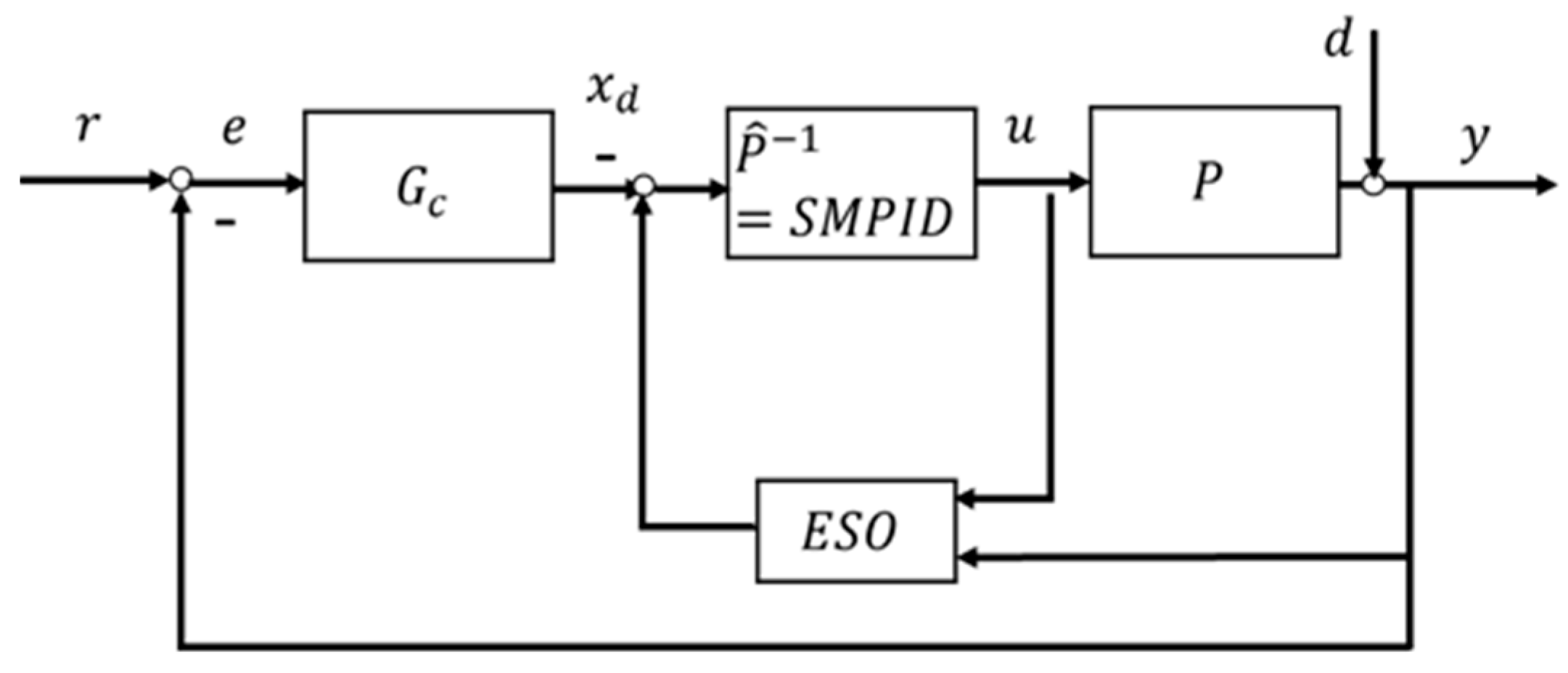
The control: Figure 2 shows the control of the model unknown plant (2).
Functionally, the control system, known as U-control, is expressed as [27]:
Σ U :   F , C C I V , P ^ 1 , P F , C I V , I n C N D I ( P ^ 1 , P ) F , C I V , I n
where F denotes the configuration of the U-control system. For a general model unknown plant P n , the objective of the U-control system is to use a double loop of control configuration with independently separate designs, taking the inner loop for nonlinear dynamic inversion/cancellation C N D I ( P ^ 1 , P ) via a model-free sliding mode control P ^ 1 = M F S M C = S M P I D to achieve the nth order identity matrix C N D I ( P ^ 1 , P ) I n , and taking the outer loop for linear dynamic inversion to realise a specified whole control system performance via a linear invariant controller G c ζ , ω n . Further, the invariant controller generates the desired state vector for the inner state feedback control loop. For state feedback control, if full states are not available, a state observer, for example, extended state observe ( E S O ), can be used for the state estimate from the controller input and the measured system output [34]. This study uses the U-control platform to conduct simulation demonstrations of the newly proposed SMPID control for the whole control system’s performance.
Remark 1. 
A similar idea has appeared in the work on online adaptive tuning for PID controllers [35]. It proposes two adaptive loops. To guarantee the robust stability of the system in the first loop (the inner loop), the controller is evaluated and tuned online without betting against nominal design performance. The second loop (outer loop) performs periodic on-line detection when modelling errors occur and retunes the controller. After this, the system is treated as a newly configured system to provide effective control performance directly. This is also the U-control configuration with a double loop, but the difference is that the inner loop in U-control takes robust NDI, so the outer loop design with the specified system performance is completely independent from the inner loop design. In addition, U-control is a complete model-free approach, so there is no need for adaptively estimating some extra information for designing controllers.

2.2. SMC

Setting up the sliding mode function is important for deriving the control input and the whole control system’s performance. Various options have been well developed, such as Fillipov’s approach and the equivalent control approach [36,37]. This study uses the equivalent control method as a foundation for the follow-up analyses.
For designing SMC, define a sliding mode function in the form of [38]
σ ( x ˜ ) = C x ˜ :   n
where x ˜ = x x d = x ˜ x ˜ ˙ x ˜ ( n 1 ) T n is the state tracking error vector, and from (2) x = x 1 = y x 2 = y ˙ x n 1 = y ( n 1 ) T n , and x d = x d x ˙ d x d ( n 1 ) T n are the state vector and the desired state vector, respectively, C 1 n is assigned to make the sliding mode function a Hurwitz stable polynomial σ ( x ˜ ) = C x ˜ = 0 .
For determining the corresponding controller outputs in practise, set up a sliding mode boundary layer thickness δ around the sliding mode. Correspondingly, the switching controller u s w and the equivalent controller u e q are formulated as
u = u s w = k g sgn ( σ ) σ δ u e q = η ( σ ˙ = 0 ) σ δ
where η ( ) denotes a function of the plant nominal model.
Proposition. 
Regarding SMC system design (switching controller  u s w and equivalent controller  u e q ), let a Lyapunov function ( V ) satisfy the stability conditions  V = σ 2 0 V ˙ = σ ˙ σ 0 , where  σ ( x ˜ ) is the sliding function is pre-assigned, such as that given in (3). For determining the switch control  u s w , using u s w = k g sgn ( σ ) ( k g 0 M in which  inf ( f n ) = m f n ( x , u , d ) sup ( f n ) = M ) to suppress the total uncertainty. For determining the equivalent control  u e q , (1) for model-based SMC, assign  σ ˙ = 0 to solve a nominal model-based equation for  u e q , (2) for model-free SMC, assign  σ ˙ = u = ρ ( σ ) , where  ρ ( ) is a monotone bounded function of  σ , to determine  u e q σ ˙ σ 0 without refereeing the nominal model, so that the SMC is asymptotically converged,  lim t σ ( x ˜ ) 0 .

2.3. Model-Free Observer

Regarding state feedback control, when only the plant input/output are measurable, an observer is needed to estimate the plant state vector with the measured input/output. There have been various types of observers [39,40]. This study reformats a linear extended state observer (LESO) [34] into a model-free observer. Refer to plant (2), take the representation x = y ( 0 n 1 ) = x 1 = y x 2 = y ˙ x n 1 = y ( n 1 ) T n and x n = f x , u , d yield the following state observer:
x ^ ˙ j = x ^ j + 1 + ω j λ j ( y x ^ 1 ) , j = 1 , 2 , n 1 x ^ ˙ n = x ^ n + 1 + ω n λ n ( y x ^ 1 ) + u x ^ ˙ n + 1 = ω n + 1 λ n + 1 ( y x ^ 1 )
where ω is the observer bandwidth and λ j , j 1 , n + 1 are the error gains tuned by λ j = ( n + 1 ) ! j ! ( n + 1 j ) ! which satisfy the Hurwitz stability condition s + 1 n + 1 = s n + 1 + λ 1 s n + λ n s + λ n + 1 .

3. Sliding Mode Function-Based PID and Model-Free Control System Design

3.1. SMPID

Here, the general SMPID is proposed below:
σ ( x ˜ ) = C x ˜ , σ 2 0 σ ˙ = u = S M P I D ( σ ) σ ˙ σ 0 = u s w = k g sgn ( σ ) σ δ u e q = S M P I D ( σ ) σ ˙ σ 0 σ δ
where σ ( x ˜ ) is a sliding mode function, which takes a popular form of σ = c 1 e + c 2 e ˙ + + c 2 e ( n 2 ) + e ( n 1 ) e = x 1 x d e ˙ = x 2 x ˙ d e ( n 1 ) = x ( n 1 ) x d ( n 1 ) T , n , C 1 n is assigned to make σ ( x ˜ ) = 0 a Hurwitz stable polynomial, u ( t ) = S M P I D ( σ ) : u ( t ) = k p σ ( t ) + k i 0 t σ ( τ ) d τ + k d d σ ( t ) d t satisfying the Lyapunov asymptotic stability condition V 0 V ˙ = σ ˙ σ 0 .
Corollary 1. 
For satisfying the Lyapunov asymptotic stability, it requires  u σ 0 .
Proof. 
Let the Lyapunov function with asymptotic stability condition be V = 1 2 σ 2 0 V ˙ = σ ˙ σ 0 . From the 2nd line of (7), it has u = σ ˙ , therefore u σ = σ ˙ σ 0 is the standard Lyapunov condition of SMC needs satisfied.
Remark 2. 
SMPID (7) generalises conventional PID (2), that is, σ ( x ˜ ) P I D ( σ ) = x 1 x d = e ( t ) P I D ( e ) .
Remark 3. 
With the author’s best knowledge, it should be noted that the other works on the so-called ‘sliding model PID’ are a type of SMC with a PID sliding function (Eker 2006) in forms of  u = sliding - mode ( PID ( e ( t ) ) .
Remark 4. 
This is a model-free design of the SMPID; that is, there is no need for a plant parametric model in designing controller output  u as it is determined by u = S M P I D ( σ ) σ ˙ σ 0 .

3.2. SMPID Design

Theorem 1. 
For switching MFSMC, considering a sliding mode function σ ( x ˜ ) = σ ( x x d ) = σ x ˜ x ˜ ˙ x ˜ ( n 1 ) = σ ( e ) = c 1 e + c 2 e ˙ + c n 2 e ( n 2 ) + e ( n 1 ) , there exist some control functions with  σ ˙ = u = S M P I D ( σ ) σ ˙ σ 0 can stabilise the plant model-free control systems to achieve  lim t σ ( x ˜ ) 0 :   lim t x ˜ = x x d 0 and dynamic inversion  C N D I ( P ^ 1 , P ) a s y m p I n .
Proof. 
The proof considers three types of controllers, P, PI, and PID from the general SMPID u ( t ) = S M P I D ( σ ) : u ( t ) = k p σ ( t ) + k i 0 t σ ( τ ) d τ + k d d σ ( t ) d t , plus a continuous nonlinear controller u = k h tanh ( k 0 σ ) .
  • Proportional (P) function
Consider
σ ˙ = u = u s w = k g sgn ( σ ) σ δ u e q = k l σ σ δ
where constant gains k g 0 ,   k l 0 . The corresponding Lyapunov functions satisfy the following stabilisation conditions:
V = σ 2 0 V ˙ = σ ˙ σ = k g sgn ( σ ) σ 0 , sup ( k ) k g u s w k l σ 2 0 , sup ( k ) k l u e q
where sup ( k ) is the plant bound, and sup ( k g ) , sup ( k l ) are the stability bounds of the controllers, respectively. Therefore lim t σ ( x ˜ ) 0 :   lim t x ˜ = x x d 0 .
  • Proportional and Integral (PI) functions
Consider
σ ˙ = u = u s w = k g sgn ( σ ) σ δ u e q = k p σ k i σ σ δ
where the constant gains k p 0 ,   k i 0 . Therefore, the Lyapunov functions have the following stabilisation conditions satisfied with:
V = σ 2 0 V ˙ = σ ˙ σ = k g sgn ( σ ) σ 0 , sup ( k ) k g u s w k p σ 2 k i σ σ 0 , sup ( k ) k p + k i k p k i , k p σ 2 k i σ σ u e q
where sup ( k ) is the plant bound, and k g , k p , k i are the stability bounds of the controllers, respectively. Therefore lim t σ ( x ˜ ) 0 :   lim t x ˜ = x x d 0 .
  • Proportional, Integral, and Derivative (PID) functions
The PID function can be expressed as
σ ˙ = u = ρ ( σ ) u ( t ) = k p σ ( t ) + k i 0 t σ ( τ ) d τ + k d d σ ( t ) d t = k p σ ( t ) + k i 0 t σ ( τ ) d τ + k d σ ˙
Accordingly, it gives,
( 1 k d ) σ ˙ = k p σ ( t ) + k i 0 t σ ( τ ) d τ
Therefore, the proof of Lyapunov stability follows that presented with the PI function above.
For the dynamic inversion C N D I ( P ^ 1 , P ) a s y m p I n in all the cases above, because lim t σ ( x ˜ ) 0 :   lim t x ˜ = x x d 0 implies x = I n x d .
Remark 5. 
Regarding PI control, the second line conditions of the equivalent control are particularly true while the trajectory approaching the sliding mode,  σ 1 because  k p σ 2 k i σ σ = k p σ 2 k i 2 σ 3 σ 1 0 .
  • Nonlinear function σ ˙ = u = ρ ( σ )
It has been observed that variable structure (as switch control is used) in SMC has side effects (inducing chattering effects) in terms of smooth control. This study proposes a nonlinear function of u = ρ ( σ ) to avoid such switching control while keeping the similar characteristics of the model-free SMC in terms of smooth (non-switching) control.
Theorem 2. 
(Non-switching/continuous MFSMC): There exist some bounded monotone functions that can approximately cover both controllers  u s w and  u e q designs in a continuous relationship of  σ ˙ = u = ρ ( σ ) to make  lim t σ ( x ˜ ) 0 :   lim t x ˜ = x x d 0 and dynamic inversion  C N D I ( P ^ 1 , P ) a s y m p I n .
Proof. 
Definite a bounded monotone function  ρ on A   ρ : A E ( A E ) , it has a bounded left and a bounded right limit at each point  σ . If  ρ (monotonically increasing) on an interval  σ ( a , b ) 0 , then  ρ ( σ ) = sup ρ ( σ ) , σ ( a , b ] a σ b , otherwise  ρ (monotonically decreasing) on an interval  σ ( a , b ) 0 , then ρ ( σ + ) = inf ρ ( σ ) , σ [ a , b ) a σ b . Let the Lyapunov function  V = 1 2 σ 2 , hence its derivative is derived as  V ˙ = σ ˙ σ . For satisfying the SMC with asymptotic stability, it requires  V = σ 2 0 V ˙ = σ ˙ σ = ρ ( σ ) σ 0 . Obviously, the first condition is naturally satisfied with  V 0 , for the second condition  V ˙ = σ ˙ σ = ρ ( σ ) σ , it is still a bounded monotone function, assign  ρ ( σ ) = k h ρ ( σ ) , k h 0 so that  V ˙ = σ ˙ σ = k h ρ ( σ ) σ 0 . Therefore  lim t σ ( x ˜ ) 0 :   lim t x ˜ = x x d 0 and  x = I n x d C N D I ( P ^ 1 , P ) a s y m p I n .
This study uses a monotone-bounded hyperbolic tangent function for continuous SMC. Consequently, the Lyapunov asymptotic stability is conditionally satisfied below,
V = σ 2 0 V ˙ = σ ˙ σ = k h tanh ( k 0 σ ) σ 0 , sup ( k ) k h sup ( k h )
where sup ( k ) is the plant bound and sup ( k h ) is the stability bound of the controller. The constant gains k h 0 and k 0 0 jointly regulate the controller amplitude and convergent speed. Accordingly, the non-switching (continuous) SMC output is formulated as σ ˙ = u = ρ ( σ ) = k h tanh ( k 0 σ ) u e q = u s w u .
Remark 6. 
It should be noted that there are various choices for such bounded monotone functions acting as continuous SMC (CSMC), such as sigmoid functions [41]. Such CSMC can be changed to conventional SMC by introducing a switching control, but it has some difficulty regulating the control performance. Regarding online applications, better use SMPID types of controllers because those transcendental functions take more time in computation and very possibly induce large numerical errors.
Remark 7. 
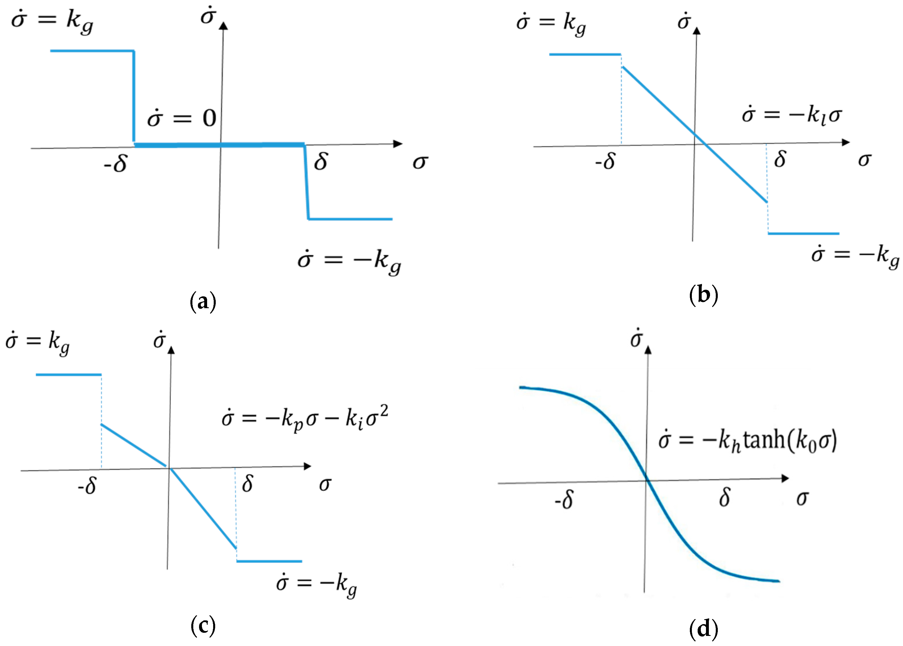
Figure 3 illustrates the relationship of  σ ˙ = ρ ( σ ) for the proposed controllers in sliding coordinate system. Figure 3a indicates a non-smooth relationship of  σ ˙ = ρ ( σ ) which is the case with the conventional switching SMC. Figure 3b–c show variable structure control using the switching control. Figure 3b–d show smooth monotonic within the sliding mode bands. O inspection of Figure 3d, it shows the monotone-bounded hyperbolic tangent function (tanh). Compare it with Figure 3b, and it is noted that (1) the height gain  k h is equivalent to the switch amplitude of  u s w in Figure 3b; (2) the width gain  k 0 corresponds to  k l in Figure 3b; and (3) The tanh function smoothly covers both switching and equivalent controls in Figure 3b; therefore, the nonlinear function provides a smooth and model-free SMC.

3.3. Analysis of Convergence

Corollary 2. 
Let ε ( t ) , σ = c o n s t , ε ( t ) = c o n s t , is a virtual variable for matching the differential equation. The selected sliding mode functions with the above-proposed SMPID controllers have the following convergence properties:
(1)
For the SMP controller, within the sliding bands, locally, its sliding mode function monotonically exponentially converges with lim σ ( t ) t = ε k l k or lim σ ( t ) t ε k l k = 0 .
(2)
For the SMPI controller, within the sliding bands, locally, its sliding mode function monotonically exponentially converges with lim σ ( t ) t = 0 .
(3)
For the nonlinear (with tanh) control, globally its sliding mode function monotonically converges with lim σ ( t ) t = 0 .
Proof. 
 
(1)
For SMP, it has been proven [27].
(2)
For SMPI, take the Laplace transform of σ ˙ = ( k p k 1 ) σ ( k i k 2 ) σ + ε to yield σ ε = s s 2 + ( k p k 1 ) s + ( k i k 2 ) = s ( s + p 1 ) ( s + p 2 ) , where poles p 1 , p 2 are negative (stable) and real (monotonic) conditioned with k p k 1 0 , k i k 2 0 and k p k 1 2 4 k i k 2 . The corresponding step response is σ ( t ) = p 1 ( p 1 p 2 ) exp ( p 1 t ) + p 2 ( p 2 p 1 ) exp ( p 2 t ) . Therefore, the sliding mode function is monotonically exponentially converged with lim σ ( t ) t = 0 . This can be proved by taking up the Laplace transform final value theorem as well.
(3)
For nonlinear systems (with tanh), it is difficult to obtain the global differential equation solutions. Heuristically, from the properties of the tanh function, it is monotonic and tanh ( σ ˙ ) = exp ( σ ) exp ( σ ) exp ( σ ) + exp ( σ ) σ = 0 = 0 .

3.4. Analysis of Robustness and Chattering

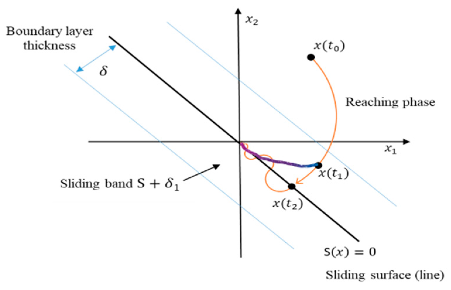
Figure 4 [27] shows the trajectories of the conventional SMC and the MFSMC (Red SMC and Red + Blue for MFSMC) on the phase plane.
The MFSMC has much stronger robustness compared with those model-based approaches. This is because the SMC using the nominal model to determine the equivalent control deals with the percentage of uncertainty with U C N M + U C 100 % ( U C and N M are the absolute values of uncertainty and the nominal model, respectively), and the MFSMC deals with N M + U C N M + U C = 100 % uncertainty in design.
Dealing with the chattering effect is a by-product of the MFSMC.
(1)
As the MFSMC ( V = 1 2 σ 2 0 V ˙ = σ ˙ σ 0 in terms of asymptotic stability) is smoothly converged within the sliding model band, the sliding mode band can be relaxed to a reasonably larger thickness without losing performance against conventional SMC ( V = 1 2 σ 2 0 V ˙ = σ ˙ σ = 0 in terms of stability). Accordingly, reduce the chattering effects and relax the sliding band thickness setup without losing accuracy.
(2)
If the chattering effects come from unmodeled plant dynamics in equivalent controller design with the conventional SMC, then the MFSMC takes the whole plant as uncertainty in designing the equivalent controller. This could reduce the chattering effects, obviously.

3.5. Generalisation of SMC

Here, we propose a generalised SMC as an expression of
σ ( x ˜ ) = μ ( x ˜ ) t 0 ,   μ ( x ˜ ) R : n σ ˙ = u = ρ ( σ ) σ ˙ σ = 0 σ ˙ σ 0 :   m
where σ and σ ˙ are the sliding function and the derivative, respectively, x ˜ = x x d = x ˜ x ˜ ˙ x ˜ ( n 1 ) T n is the state tracking error vector, x = x x ˙ x ( n 1 ) T n , and x d = x d x ˙ d x d ( n 1 ) T n are the state vector and the desired state vector, respectively.
Proposition. 
The generalised SMC covers (1) asymptotical stabilisation and (2) finite-time stabilisation for both model-based and model-free designs.
Proof. 
The selection of the sliding function determines whether the SMC is asymptotically stabilised ( σ (   x   ˜ ) = μ ( x ˜ ) is a Hurwitz stable polynomial) or finite-time stabilised ( σ ( x ˜ ) = μ ( x ˜ ) is a fractional order stable polynomial). Regarding whether the plant model (nominal model) is used or not, for model-based, it gives u = ρ 1 ( u ) σ ˙ = ρ ( u ) = 0   σ ˙ σ = 0 , where ρ ( u ) is the nominal model, for mode-free, it gives u = ρ ( σ ) σ ˙ σ 0 without using the nominal model.
For illustration of the general representation of SMCs, the proposed SMPID can be expressed as
σ ( x ˜ ) = μ ( x ˜ ) σ ( x ˜ ) = C x ˜ Re ( λ i ) 0 σ ˙ = u = ρ ( σ ) u ( t ) = ρ ( σ ) = S M P I D ( σ ) σ ˙ σ 0
where λ i ,   i = 1 , n 1 + are the eigenvalues of the polynomial C x ˜ = 0 .
The other example [25] is selected to show off the general representation. The model-free PID continuous sliding mode controller (PID-CSMC) is designed with u ( t ) = P I D C S M C ( e ) : u ( t ) = k 1 e 1 / 3 ( t ) k 2 e ˙ 1 / 2 ( t ) k 3 0 t e ( t ) d τ . This is a special realisation of (16) in the forms of σ ( t ) = e ( t ) , and σ ˙ = u = ρ ( σ ) u = P I D C S M C ( e ) . The PID-CSMC could have another formulation by assigning σ ( x ˜ ) = C e 1 / 3 ( t ) e ˙ ( t ) T and σ ˙ = u = ρ ( σ ) u = P I D C S M C ( σ ) , which the details will be compared in future studies.

4. Case Studies

4.1. Pre-Setups

The whole control system structure is shown in Figure 2. The purpose of the simulation is to take up a series of computational demonstrations to validate the whole control system configuration in terms of functionality and numerical processes. Further, it shows off the step-by-step design/test application procedure for applications and expansions. The major objectives include the numerical validations and analyses of
(1)
the SMPID developed in dynamic inversion and facilitation of U-control configuration,
(2)
robustness of the SMPID against uncertainty and disturbance,
(3)
dealing with chattering effects,
(4)
the new PID tuning and the whole U-control system’s performance.
This simulation is composed of three packs of case studies. The first two have used a general SISO nonlinear dynamic plant,
P y ( n ) = f ( y , u , d ) : y ¨ + y y ˙ + u y ˙ + 0.6 y sin ( u ) 2 u u 3 d = 0
where y = y y ˙ T 2 , u , and d are the output vector, input, and disturbance, respectively. It should be noted that throughout the simulation process, the plant model was not used as a reference for designing the controller and state estimator. That is, the plant is treated completely as an uncertainty; only the input/output are measurable, and the dynamic order of the plant is assumed to be known in advance.
The simulation platform is shown in Figure 2, U-control system design with two dynamic inversions (DI), (1) the plant DI to convert, by MFSMC, into an identity matrix in the inner loop, and (2) the total control performance DI (resulted in the invariant controller G c ) to achieve the specified desired linear control system performance in the outer loop. In addition, G c also provides the desired reference states for the inner loop dynamic inversion.
For the first two case studies, take the following setups:
(1)
A sequence of levelled references is assigned with
r ( t ) = 2 ( 2 , 10 ] 6 ( 10 , 20 ] 0 ( 20 , 30 ] 2 ( 30 , 40 ] t
(2)
The external disturbance is assigned as a constant d ( t ) = 1 added at the output.
(3)
Select the sliding function with σ = 20 ( x 1 x d ) + ( x 2 x ˙ d ) = 20 e + e ˙ , in which the estimate vector x ^ 1 x ^ 2 T from the LESO is used to replace the plant states x 1 x 2 T in the simulation processes. Setup the sliding mode boundary thickness δ = 1 .
(4)
The control system output is specified in the outer loop via a standard linear second-order dynamic in terms of the Laplace transform.
Y R = G = G c S M C ( P ^ 1 P ) 1 + G c = G c 1 + G c = ω n 2 s 2 + 2 ζ ω n s + ω n 2 , ζ = 0.7 ω n = 5
which represents a decayed oscillatory response without steady state error to level/position references. To design the corresponding controller, taking the dynamic inversion of the closed loop transfer function gives
G c = G 1 G = ω n 2 s 2 + 2 ζ ω n s = 1 s ω n 2 s + 2 ζ ω n
Therefore, it also sets up a desired state vector with x d = x d 1 x d 2 T = 1 s ω n 2 s + 2 ζ ω n ω n 2 s + 2 ζ ω n T which is used as the reference vector for the inner loop SMC.
(5)
For state feedback control, it is requested to obtain the estimated state vector from plant (17) input/output measurements. Select a LESO below,
x ^ ˙ 1 = x ^ 2 + λ 1 ω ( y x ^ 1 ) x ^ ˙ 2 = x ^ 3 + λ 2 ω 2 ( y x ^ 1 ) + u x ^ ˙ 3 = λ 3 ω 3 ( y x ^ 1 )
For designing the observer, use a Hurwitz polynomial s + 1 n + 1 = s n + 1 + λ 1 s n + λ n s + λ n + 1 to specify the observer’s gain vector λ 3 : λ 1 λ 2 λ 3 = 3 3 1 and assign the LESO bandwidth ω = 100 . Accordingly, the characteristic polynomial of the observer is s + ω 2 + 1 .

4.2. SMPI Control—Model-Free Variable Structure SMC

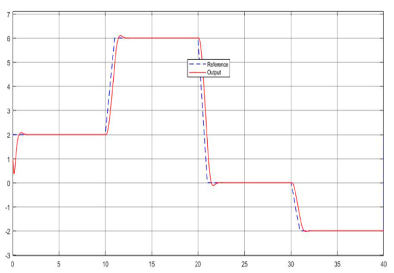
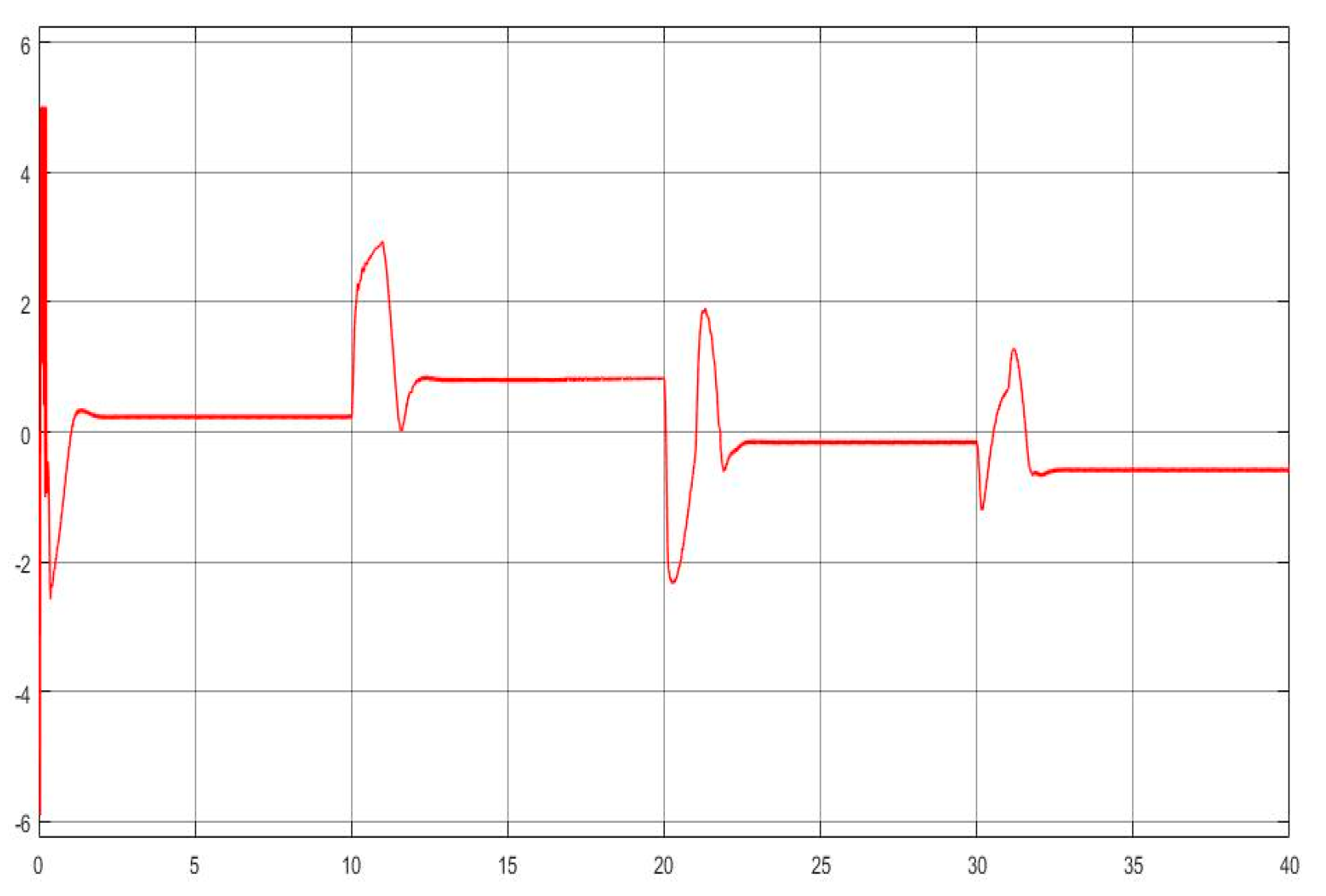
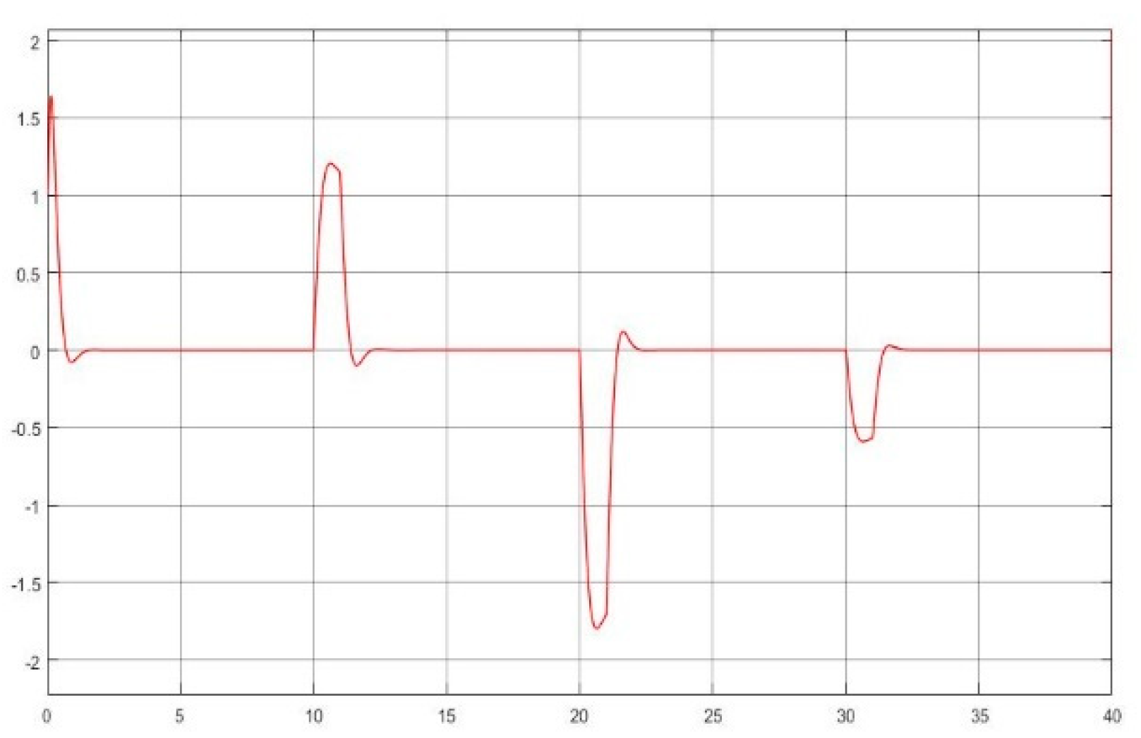
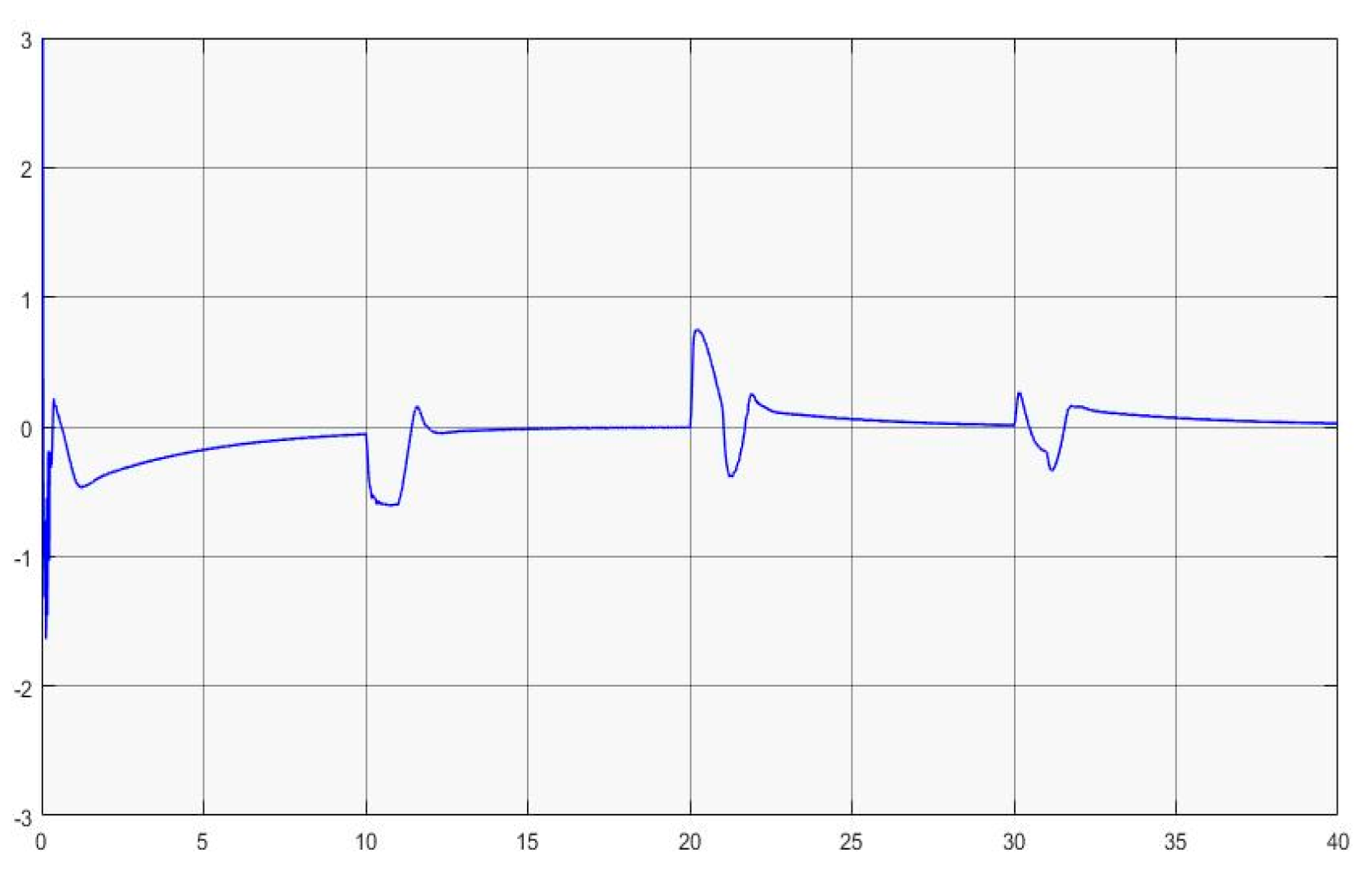
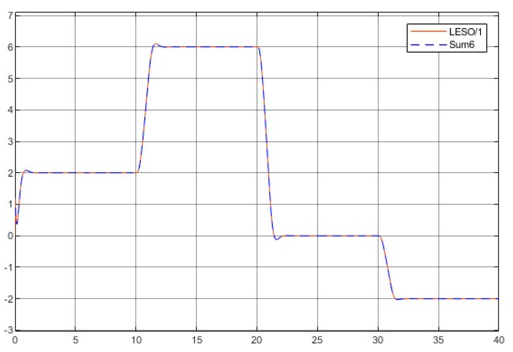
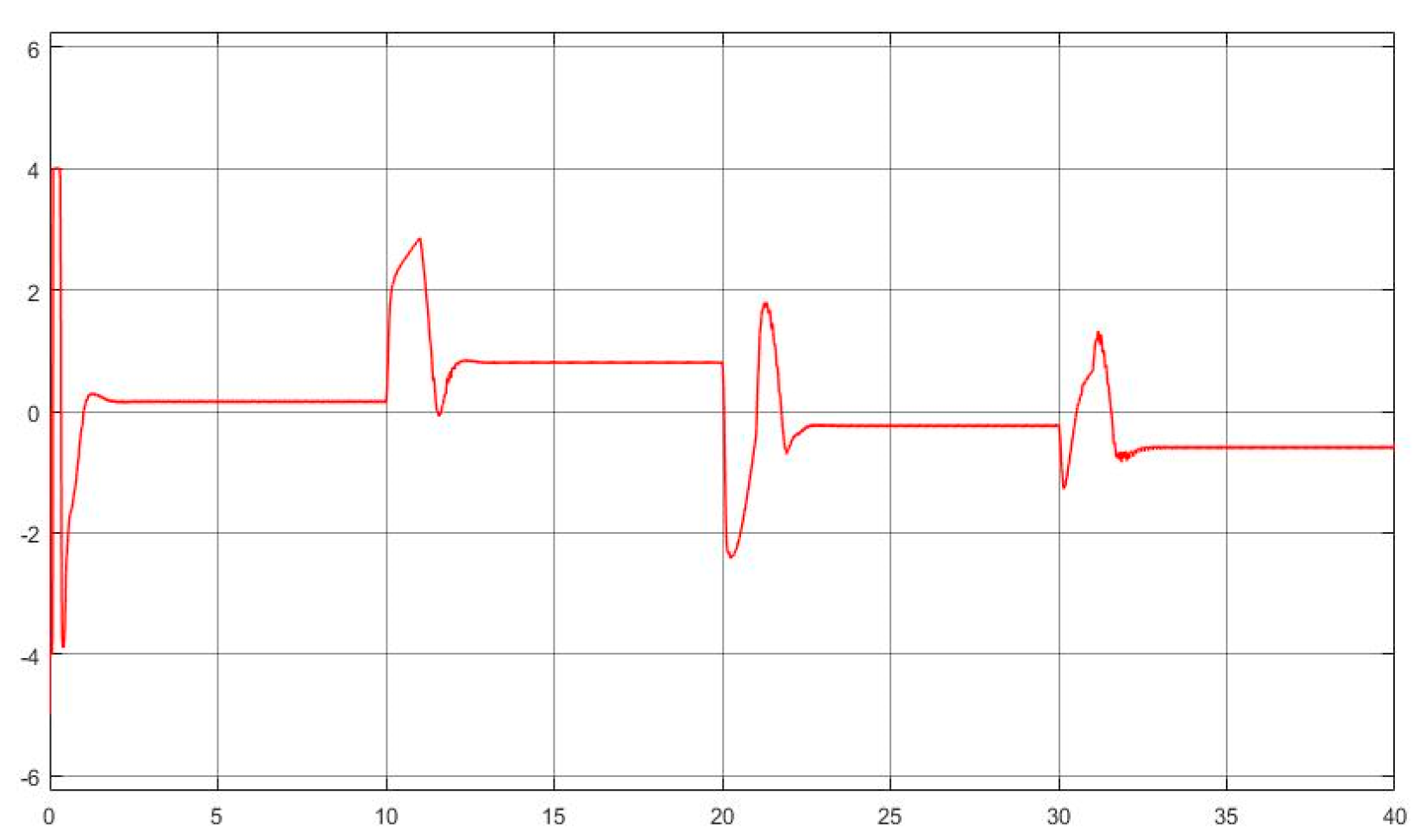
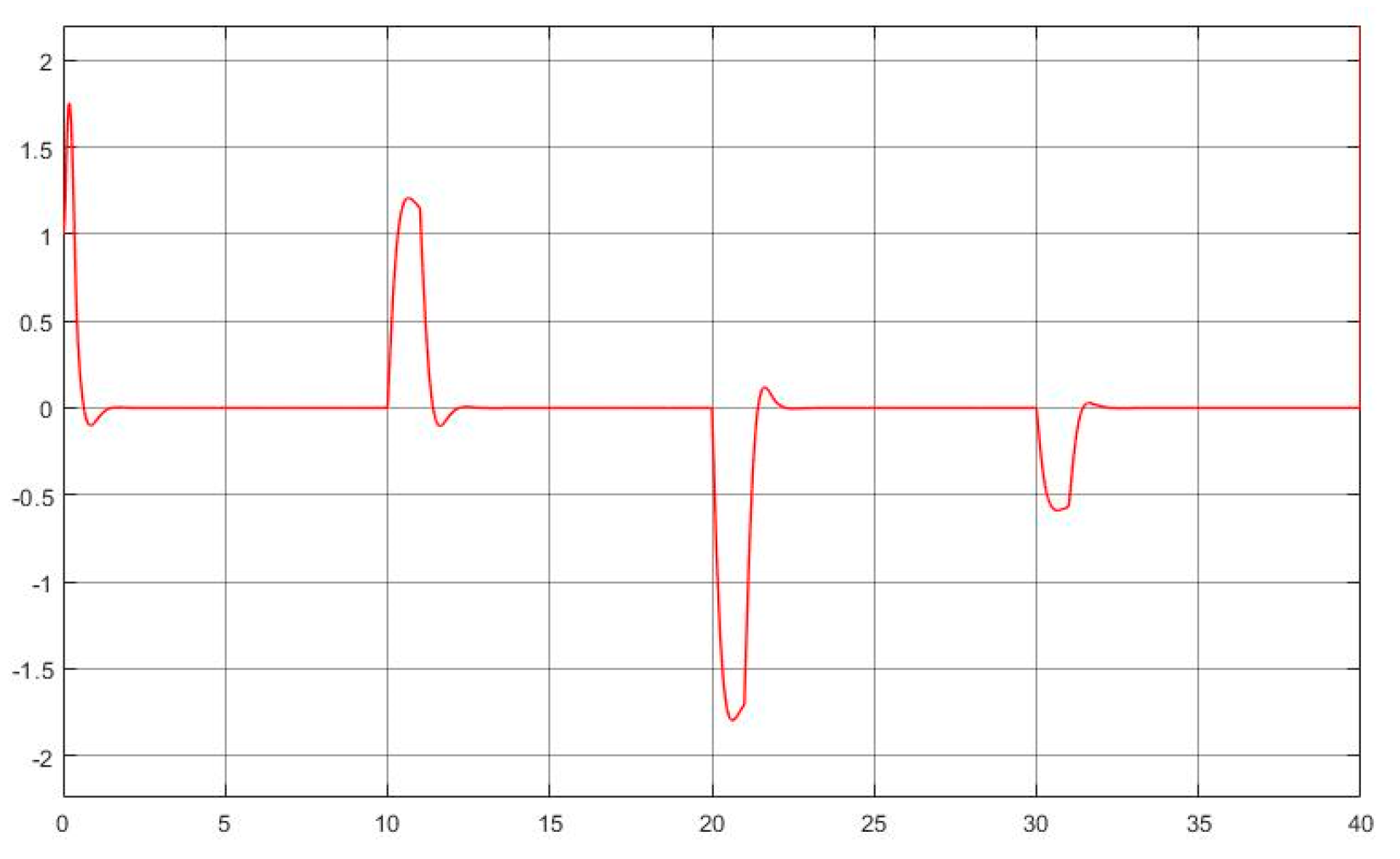
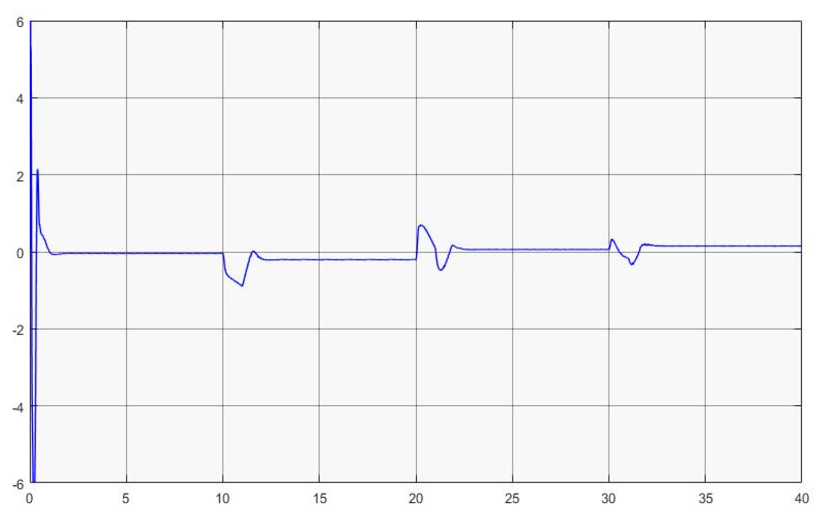
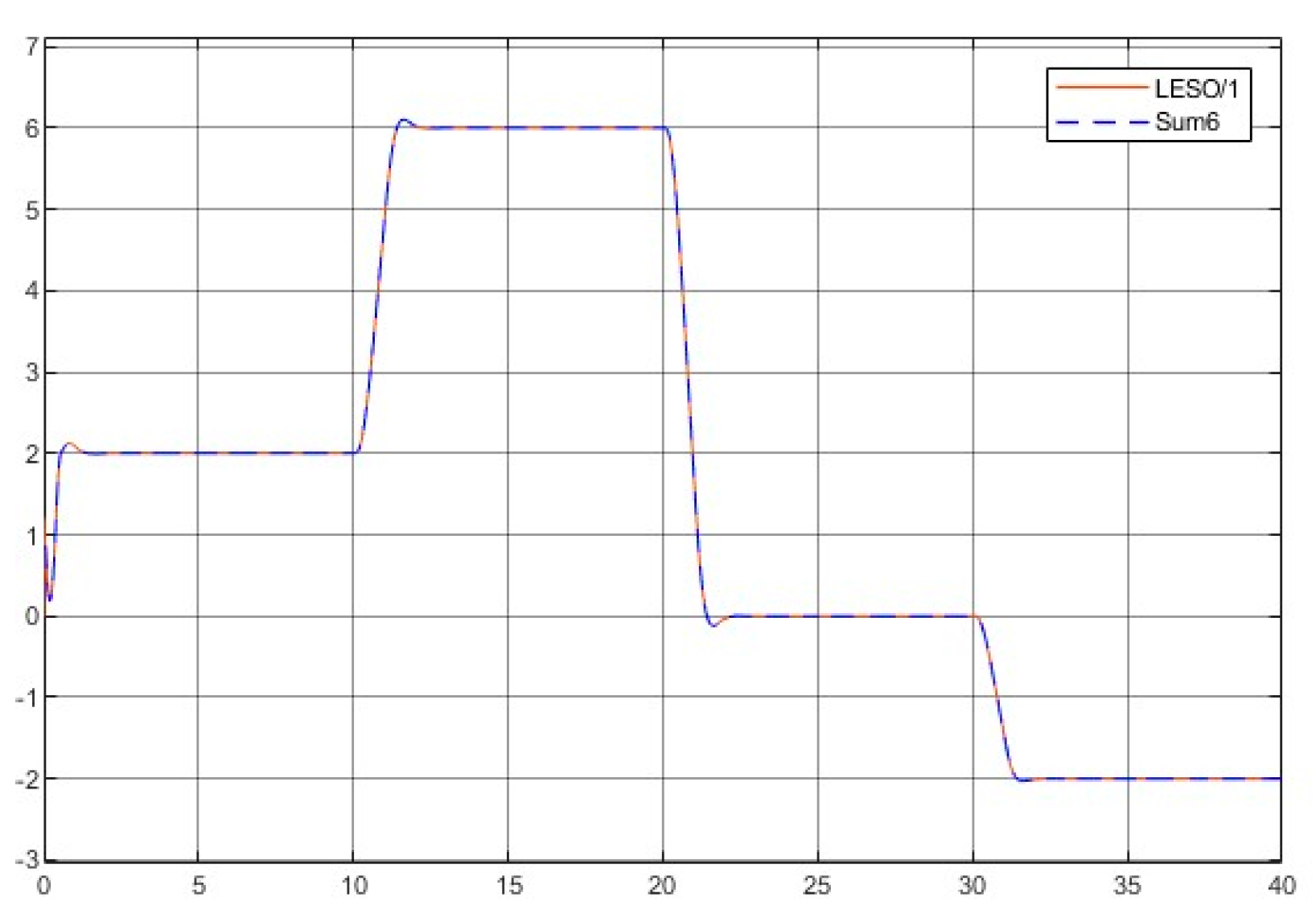
A SMPI controller is selected for the unknown plant dynamic inversion and nonlinearity cancellation in the inner loop. Accordingly, the SMPI control with u = k g sgn ( σ ) u s w k p σ k i σ u e q and k g = 5 k p = 4 k i = 1 (tuned by trial and error) are assigned to play the nonlinear dynamic inversion, which lays the foundation for achieving the U-control performance specified with the outer loop. Figure 5, Figure 6, Figure 7, Figure 8, Figure 9 and Figure 10 show off the simulated plots: Figure 5 for the system output response; Figure 6 for the control input; Figure 7 for the error sequence between the reference and the system output; Figure 8 for the sliding model function; Figure 9 for the first state and its estimate; and Figure 10 for the second state and its estimate, respectively.

4.3. SM Nonlinear P Control—Model-Free Non-Variable Structure (Non-Switching) SMC

A nonlinear SMP controller u = k h tanh ( k 0 σ ) u e q = u s w u and k h = 4 k 0 = 1 (tuned by trial and error) are assigned to place a non-switching/smooth control, which mimics the continuous SMC. Figure 11, Figure 12, Figure 13, Figure 14, Figure 15 and Figure 16 show off the simulated plots: Figure 11 for the system output response; Figure 12 for the control input; Figure 13 for the error sequence between the reference and the system output; Figure 14 for the sliding model function; Figure 15 for the first state and its estimate; and Figure 16 for the second state and its estimate, respectively.

4.4. Discussions on the Computational Demonstrations

(1)
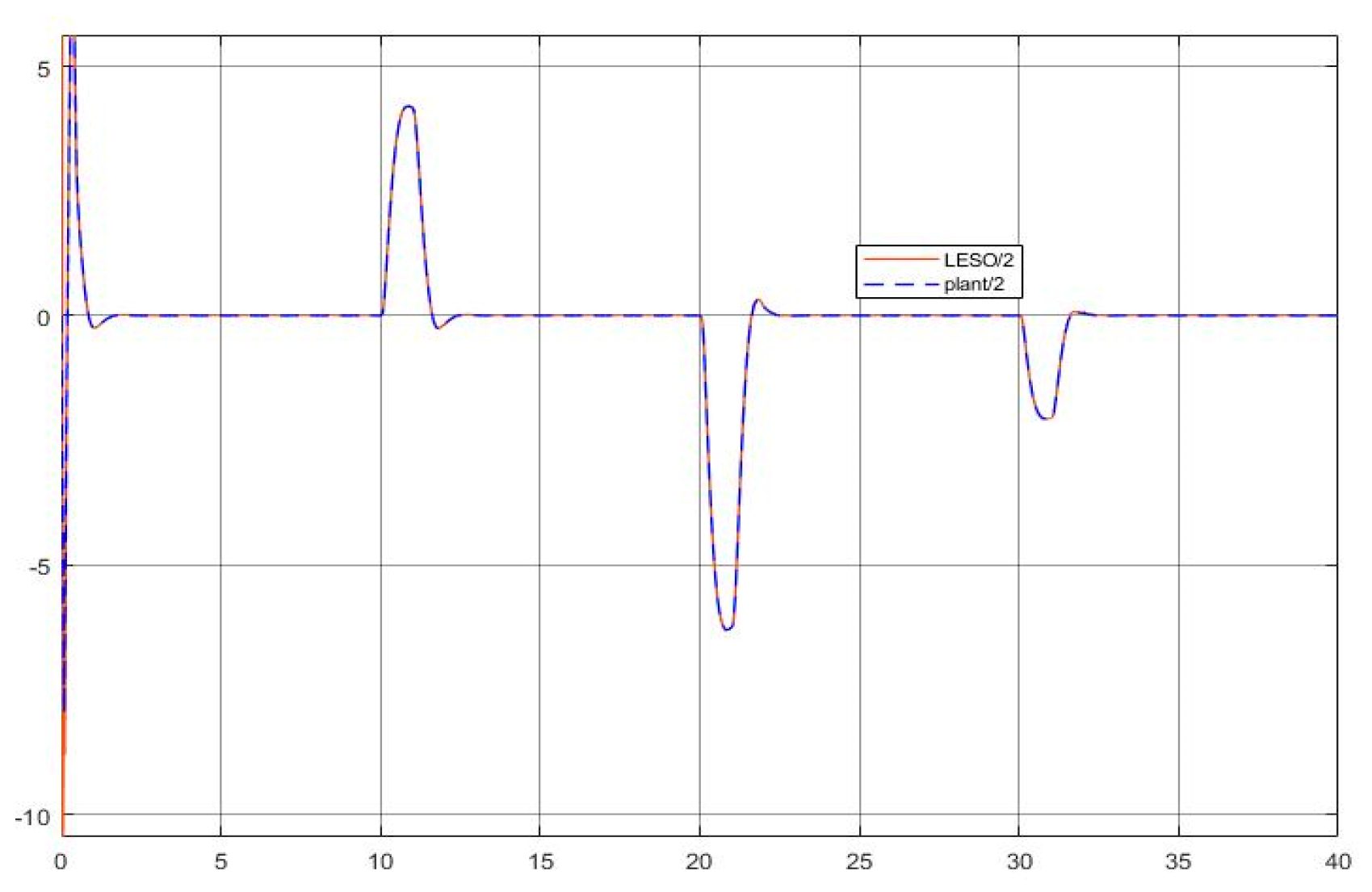
The kernel idea (in terms of two dynamic inversions, MFSMC, SMPID, LESO, and the integration of the functionalities) of the U-control is demonstrated with the first two case study plots in Figure 5, Figure 6, Figure 7, Figure 8, Figure 9, Figure 10, Figure 11, Figure 12, Figure 13, Figure 14, Figure 15 and Figure 16, which is consistent with the analytical results presented in the study.
(2)
The simulated plots in Figure 5, Figure 6, Figure 7, Figure 8, Figure 9, Figure 10, Figure 11, Figure 12, Figure 13, Figure 14, Figure 15 and Figure 16 have shown that the designed control systems can effectively drive the system states x asymptotically to achieve σ = σ ( x ˜ , t ) 0 and keep in once driven in σ = σ ( x ˜ , t ) δ with the given simulation conditions.
(3)
Total robustness against model internal uncertainty: The control system is designed to take the plant model as a whole uncertainty. Let NM be the nominal model and UC for uncertainty. The two-pack plots confirm the analysis in Section 3 that the U-control deals with N M + U C N M + U C = 100 % (total) uncertainty in design, compared with those nominal model-based designs dealing with uncertainty of U C N M + U C 100 % .
(4)
External disturbance rejection: Inspection of Figure 5, Figure 6, Figure 7, Figure 8, Figure 9, Figure 10, Figure 11, Figure 12, Figure 13, Figure 14, Figure 15 and Figure 16, the constant disturbance ( d ( t ) = 1 ) has been well suppressed, particularly in the plots show x ^ 1 x 1 and x ^ 2 x 2 in Figure 9, Figure 10, Figure 15, and Figure 16. It is noted that the estimated states from LESO have been used for the state feedback control design to deal with both uncertainty and disturbance, and jointly the inner loop (state feedback) and the external loop (output feedback) cope with the disturbance effectively. Accordingly, these efforts have achieved the desired responses.
(5)
Dealing with chattering effects at the controller output: As predicted, this performance in removing the chattering effect is mainly achieved by using asymptotically stable functions to drive the derivative of the sliding mode function σ ˙ = ρ ( σ , u ) ) a s y m p 0 once the sliding mode function enters the sliding mode band. Accordingly, the sliding mode boundary thickness δ can be assigned relatively wider without inducing steady state errors for levelled references. These are shown in Figure 6 and Figure 12. For model-based SMC, predominantly, it has been forced σ ˙ = 0 to determine the equivalent control while sliding mode functions enter the sliding mode band, where the jump/switching is the main cause of chattering with the conjunction of a narrow sliding mode band for accuracy.
(6)
Comparison of SMP control [27] and SMPI control: SMPI has removed the small steady-state error ε in the sliding mode function, which is because of the integral function introduced. This is shown in Figure 8.
(7)
Tuning of the SMPID controller gains: The simulations have tested various selections of the gains to achieve similar performance, which indicate a large range of options, under the guarantee of Lyapunov stability, feasible to make the gain tuning procedure relaxed and robustness. This is because there are many solutions for the inequality u σ 0 .
(8)
Non-switching SMC alike: The plots, in Figure 11, Figure 12, Figure 13, Figure 14, Figure 15 and Figure 16, generated from the second case study illustrate similar performance as those obtained from the first case studies. The nonlinear function u = k h tanh ( k 0 σ ) u e q = u s w u achieves good performance in the regions outside/inside of the sliding mode band. The roles of the parameters with the nonlinear function have been tested in the simulation studies, the sign of the gain k h for convergent direction and the value for convergent speed. Similarly, the width k 0 can be used to adjust the sliding mode band thickness.
(9)
The contents presented analytically and validated computationally in the study have followed a route from complexity (problems) to simplicity (analysis and solutions). The derived and simulated results are consistent and basically feasible for those with reasonably good control system knowledge to use/expand for their ad hoc research and development. In some sense, this simulation study could be treated as a user manual.

4.4.1. Comparative Demonstration (1)—Control of a Rotary Servo System

For comparing the SMPID, the third case study selects a rotary servo system having nonaffine uncertainties with uncertainty and disturbance estimator (UDE)-based robust control (UDERC) [42]. The rotary servo system has been modelled below,
θ ˙ θ ¨ = 0 1 0 25 θ θ ˙ + 0 80 u + 0 f 2 θ , θ ˙ , u + 0 d 2
where θ θ ˙ T is the angular state vector, which is measurable in the simulation, u is the control input, f 2 * = 32 θ + θ ˙ + arctan ( u ) is a nonaffine uncertainty added at the control input, and d 2 represents the external disturbance at the output. The control objective is to design a control law u to drive the system following the reference model below,
θ ˙ m θ ¨ m = 0 1 900 60 θ m θ ˙ m + 0 900 c
where θ m θ ˙ m T is the angular reference state vector, and c is the stimulating input.
For UDERC design (Ren, Zhong, and Chen 2015): It requires (1) calculating the pseudoinverse of the control input vector and (2) assigning two additional control gains in a long control function so that it achieves (1) the cancellation of the known system dynamics in the nominal model to remove the effect of mixing up with the other control functions, (2) the desired performance specified in the reference model, and (3) stronger robustness by using proportional-integral-like functions to regulate the errors. For the U-control: The SMPI is used for the NDI with a gain vector k g = 8 k p = 7 k i = 1 . Both control system performances are specified with (23).
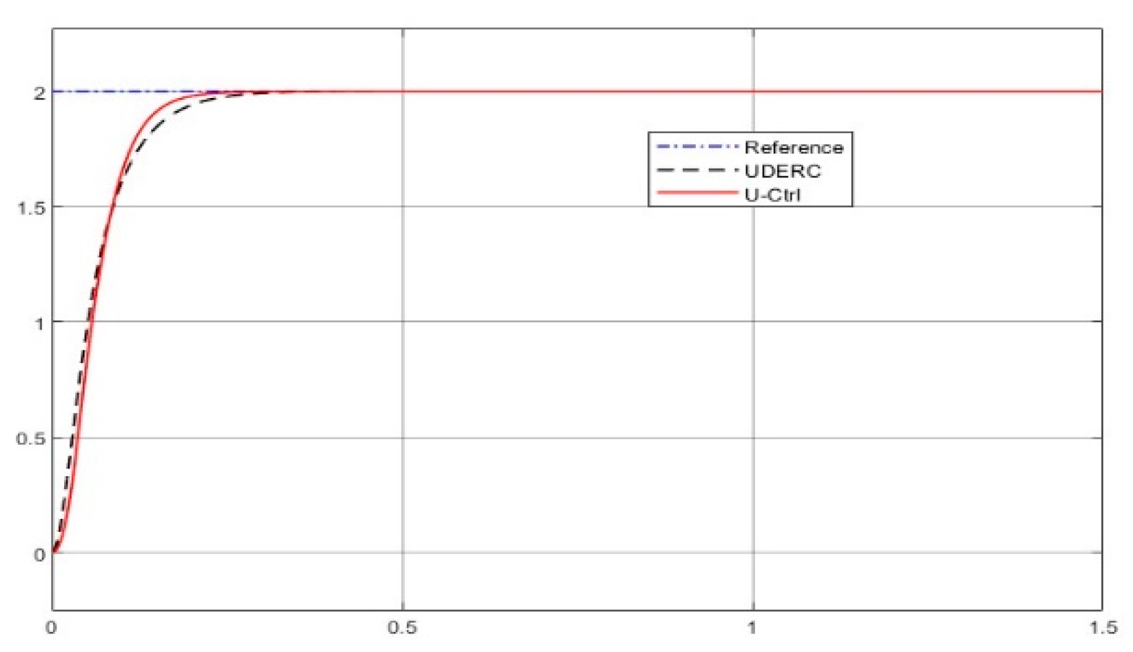
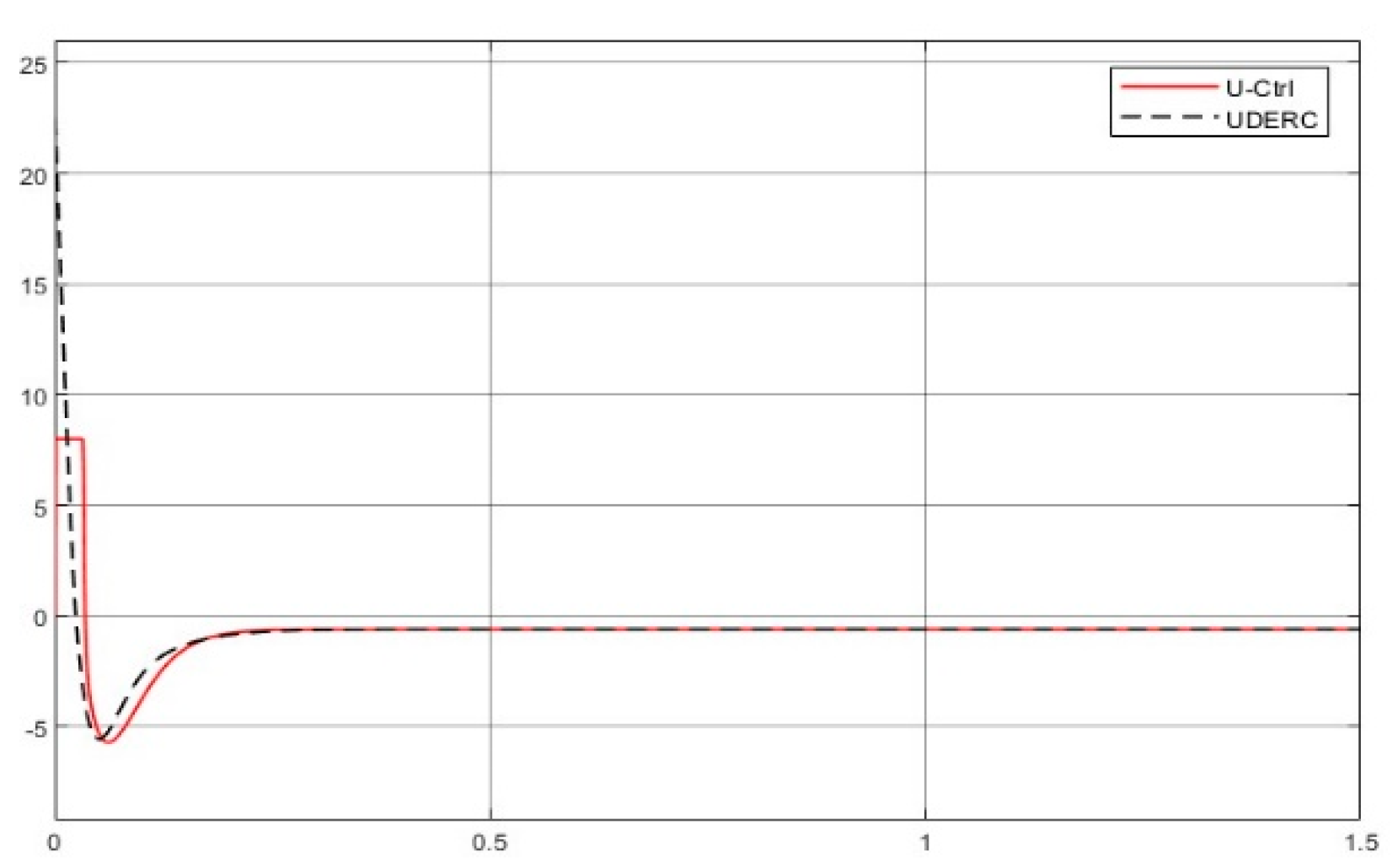
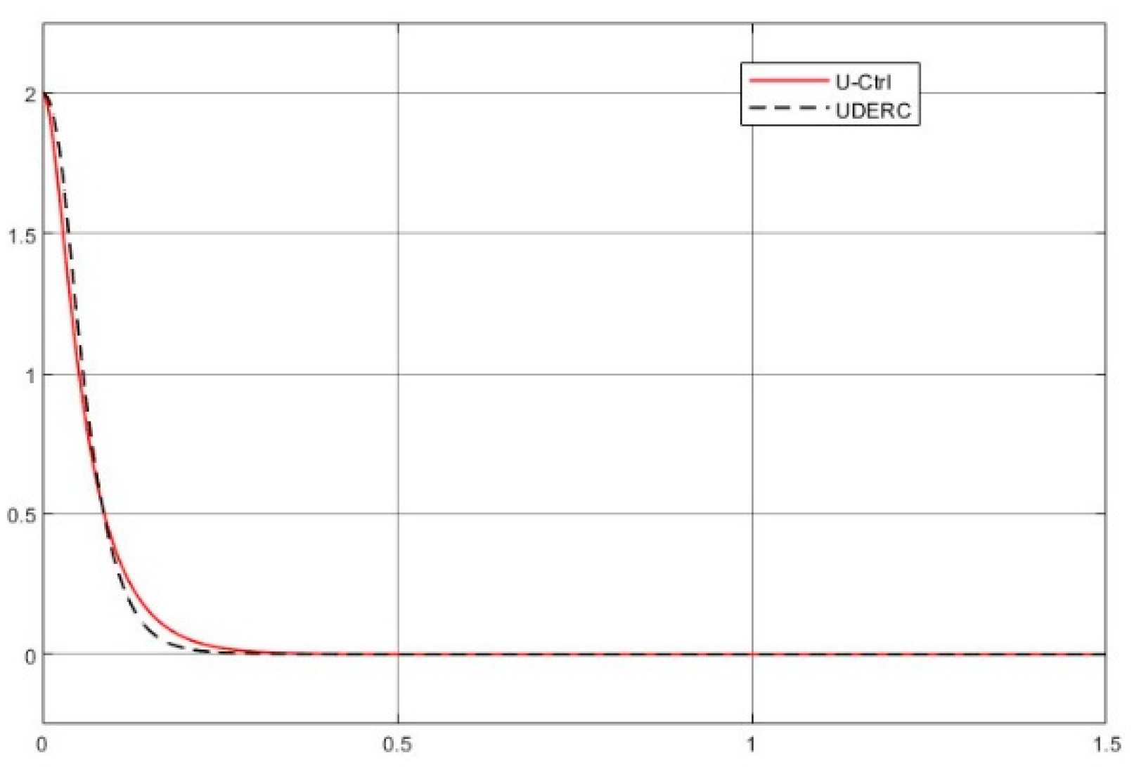
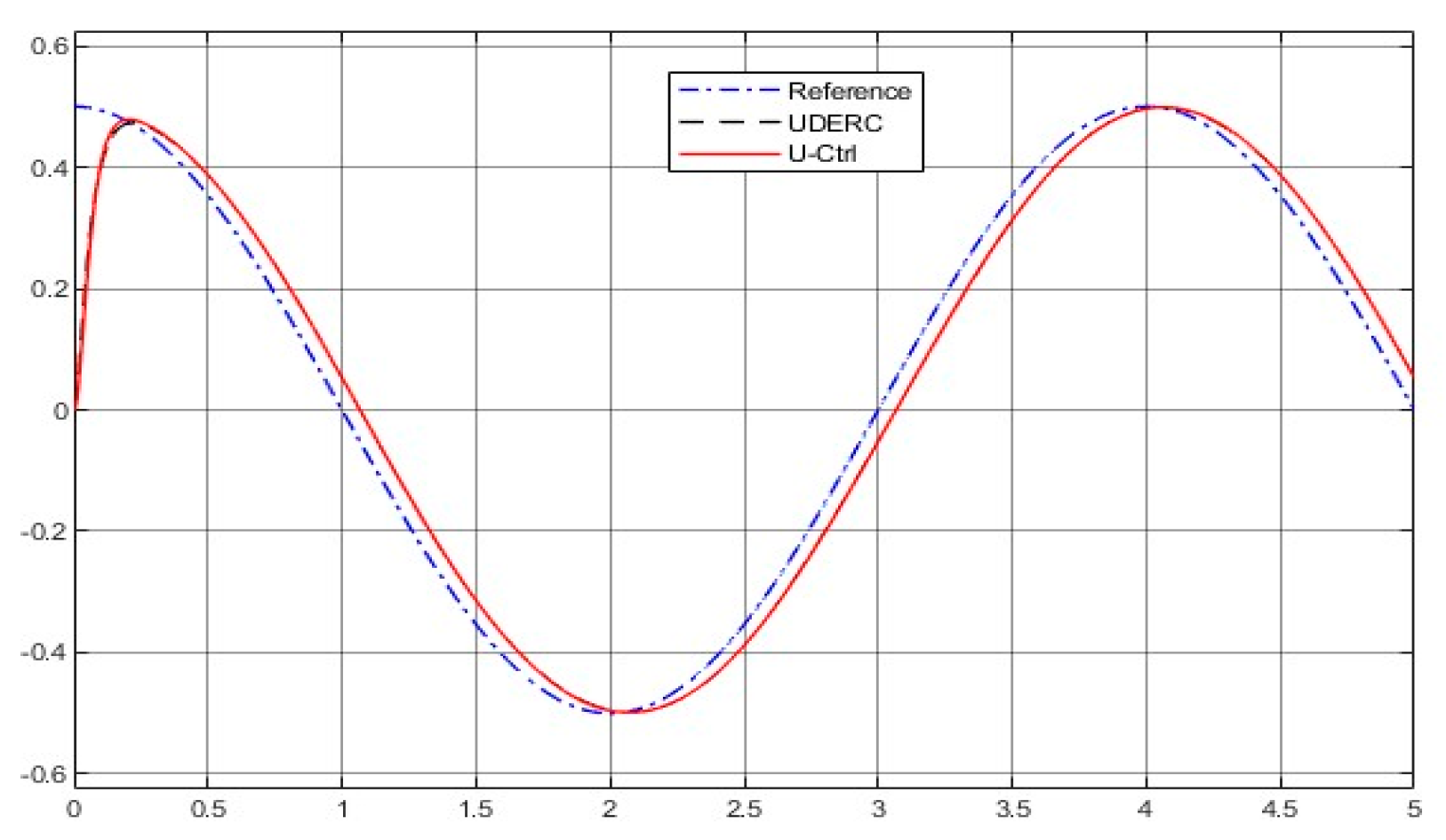
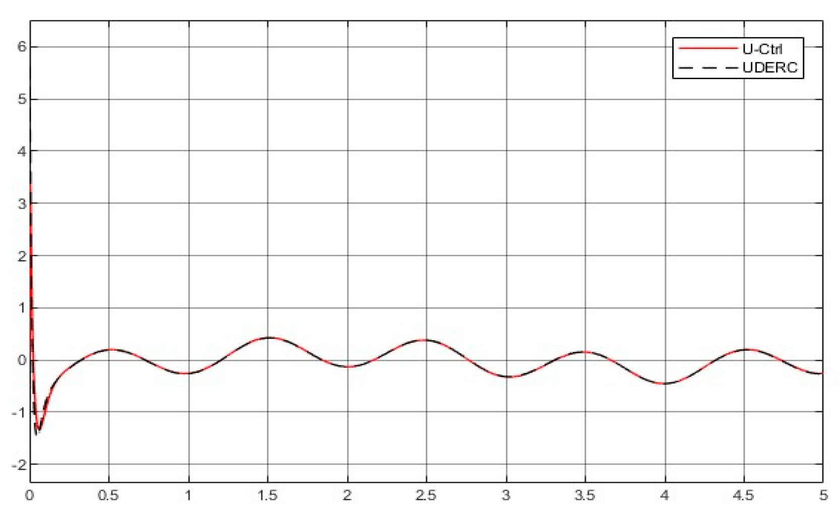
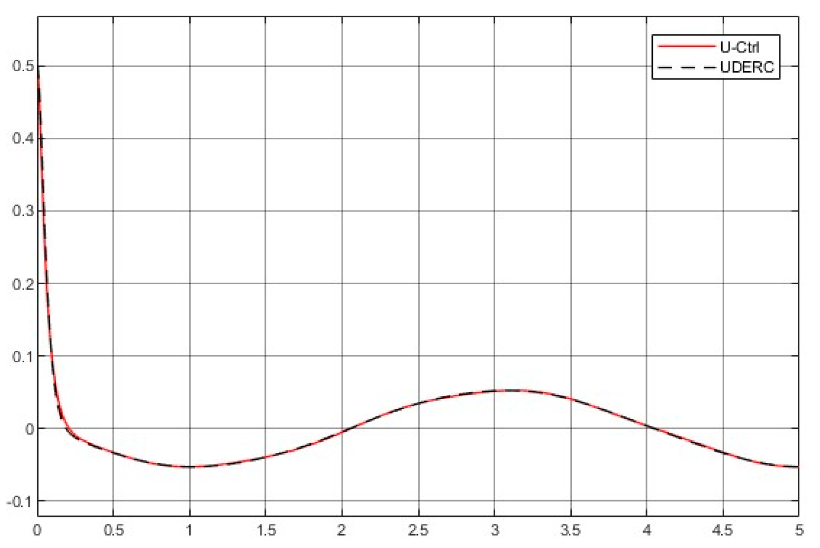
For the simulation: Test 1: Tracking a step reference without the external disturbance, that is d 2 ( t ) = 0 . Figure 17, Figure 18 and Figure 19 show off the comparative plots generated from the two control approaches: Figure 17 for the system output responses, Figure 18 for the control inputs, and Figure 19 for the error sequences between the references and the system outputs, respectively. Test 2: Tracking a sinusoidal 0.5 cos ( 0.5 π t ) reference with external disturbance d 2 = 32 cos ( 2 π t ) . Figure 20, Figure 21 and Figure 22 show off the comparative plots generated from the two control approaches: Figure 20 for the system output responses, Figure 21 for the control inputs, and Figure 22 for the error sequences between the references and the system outputs, respectively.
  • Comparison of the simulated plots
(1)
Both control approaches can achieve the same specified control objectives, as shown in Figure 17, Figure 18, Figure 19, Figure 20, Figure 21 and Figure 22.
(2)
Regarding design procedure, the UDERC requests three designs: plant dynamic inversion, desired performance implementation, and uncertainty estimation/rejection. The U-control takes two dynamic inversions and is repetitively used for both case studies. Basically, the UDERC is model-based design, and the U-control is model-free design without traditional iterative learning routines.
(3)
Knowledge request of uncertainties and disturbances, the UDERC needs a filter to estimate the uncertainty, and the U-control only needs the assumption that the unknown bound exists.

4.4.2. Comparative Demonstration (2)—Two Types of SMPIDs for Finite Time Control

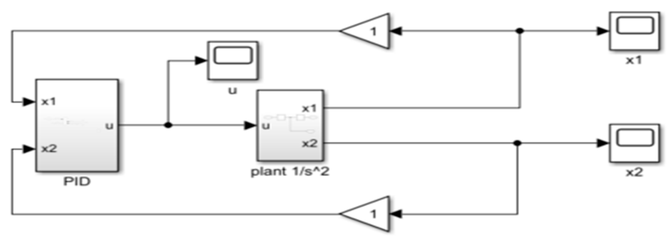
A simple example (Pérez-Ventura, Mendoza-Avila, and Fridman 2021) selected is a control system with a simple 2nd-order dynamic plant ( 1 s 2 in forms of the transfer function with initial state x ( 0 ) = 1 0 T ), and Figure 23 shows the system simulation (Simulink) block diagram. This demonstration compares two types of sliding mode based PIDs:
(1)
PID-CSMC [25]
u ( t ) = P I D C S M C ( e ) : u ( t ) = k 1 e 1 / 3 ( t ) k 2 e ˙ 1 / 2 ( t ) k 3 0 t e ( τ ) d τ k 1 = 2.7 Δ 2 / 3 k 2 = 5.345 Δ 1 / 2 k 3 = 1.1 Δ Δ = 5 = 7 . 8948 11 . 9518 5 . 5
(2)
SMP and SMPI presented in this study in terms of u = S M P I D ( σ ( e ) ) = P I D ( sliding - mode )
SMP : u = k p ( σ ( e ) ) k p = 4 σ ( e ) = 0.8 e 1 / 3 + e ˙
SMPI : u = k p σ ( e ) k p = 4 k i 0 t σ ( τ ) d τ k i = 0.8 σ ( e ) = 0.8 e 1 / 3 + e ˙
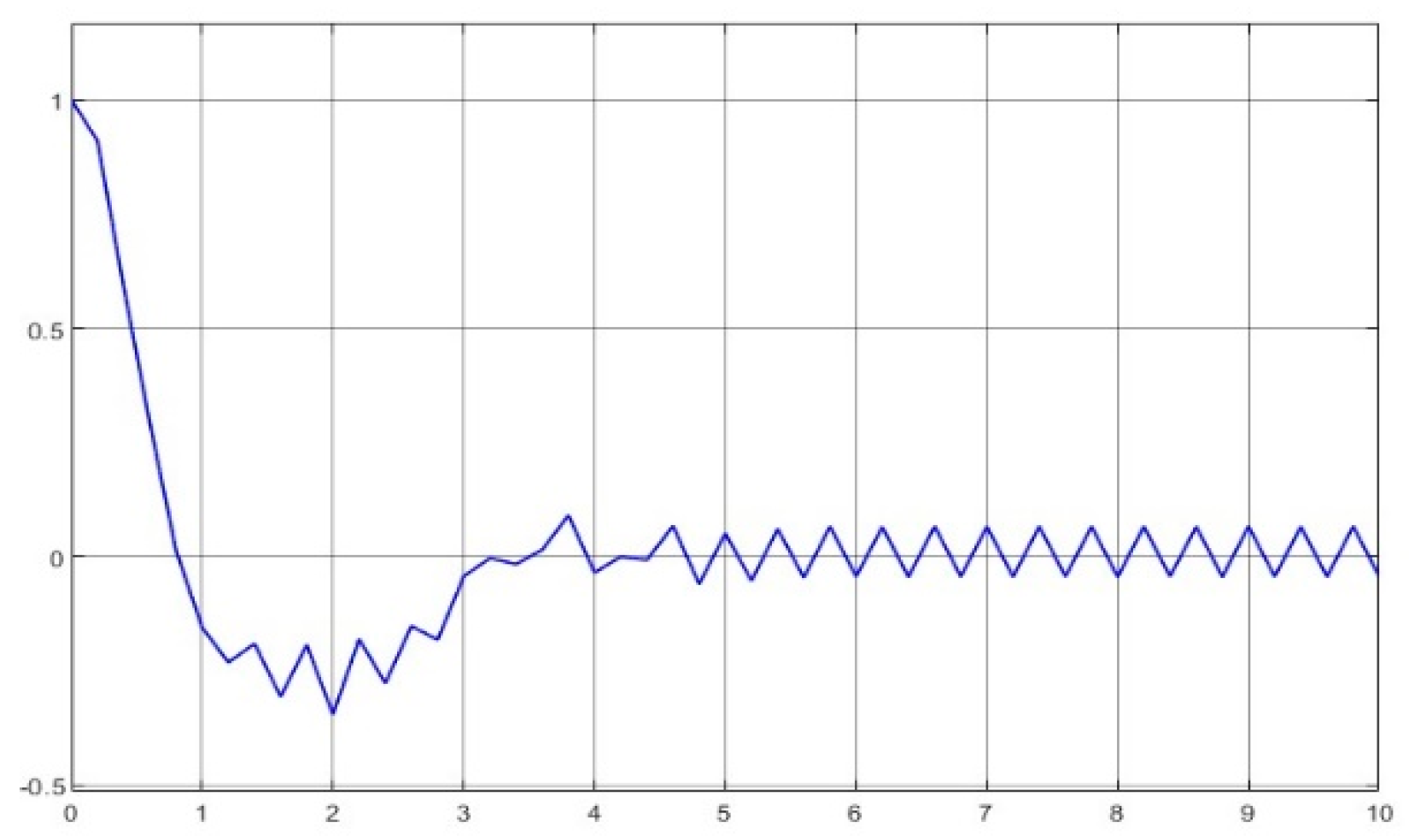
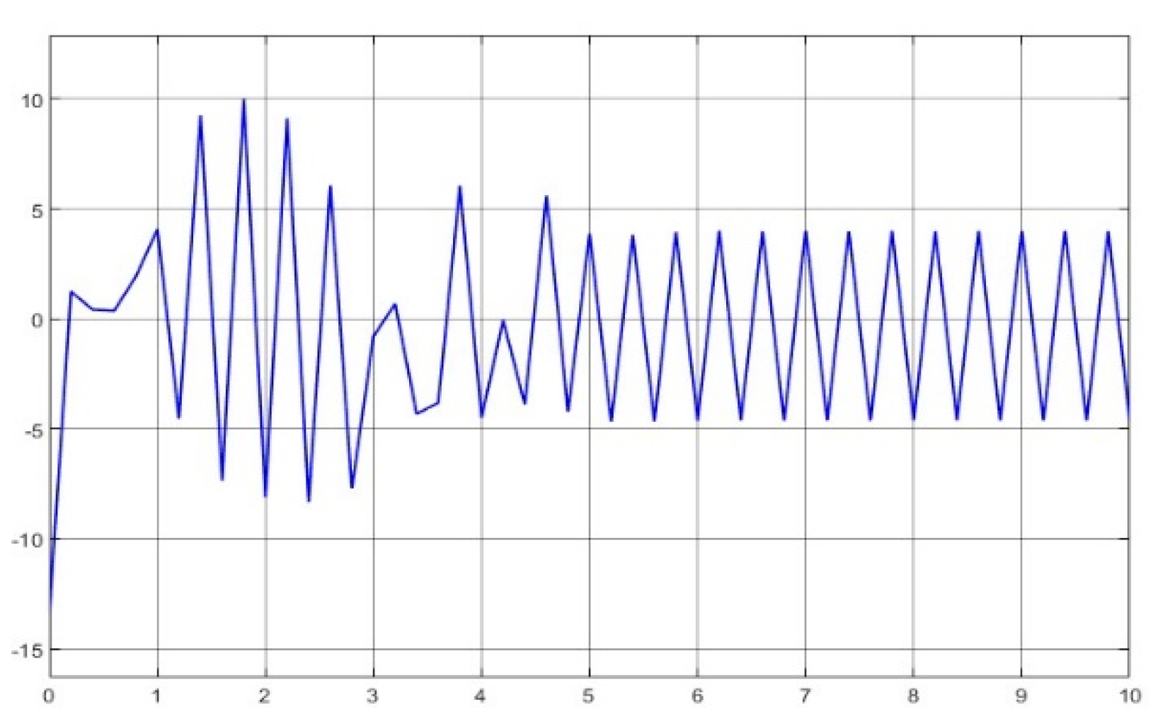
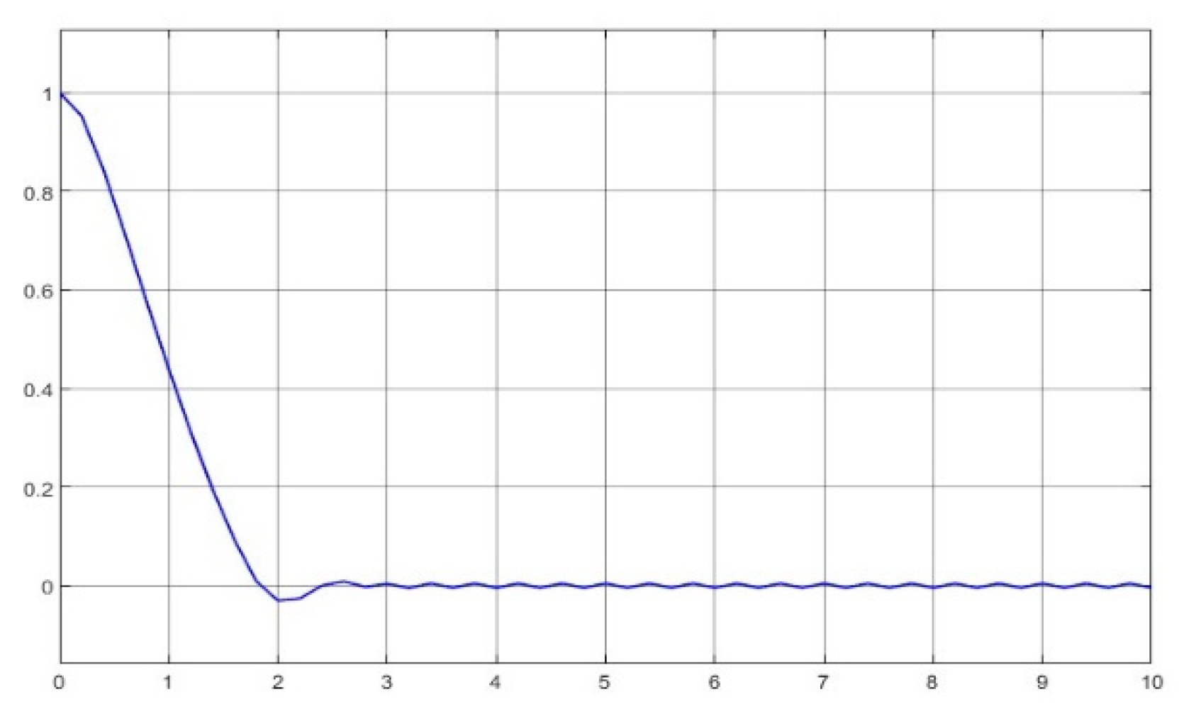
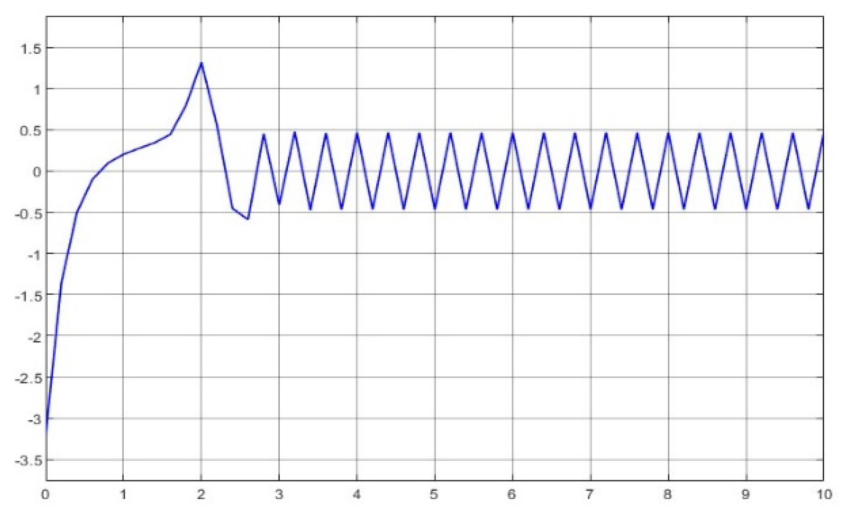
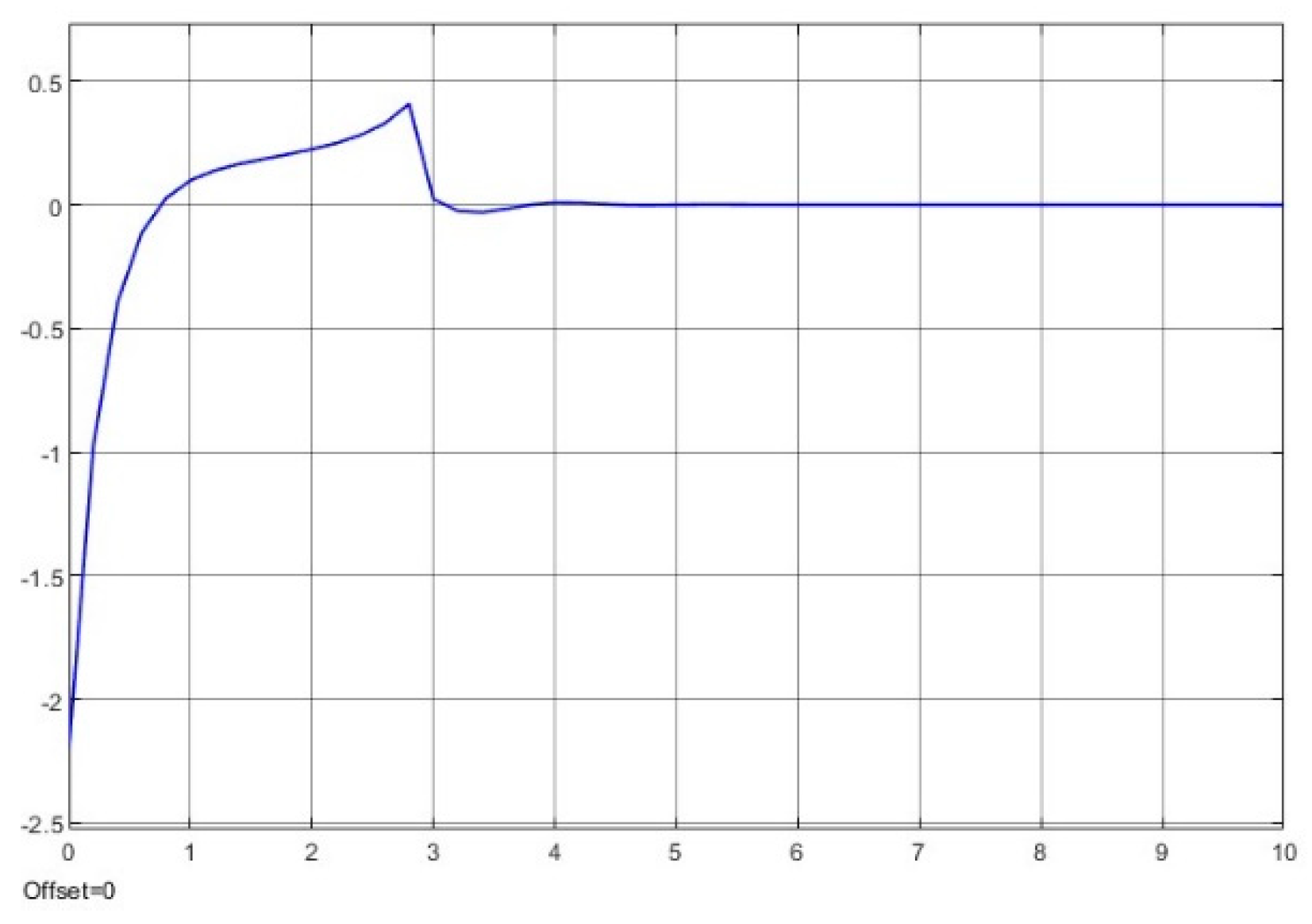
Figure 24, Figure 25, Figure 26, Figure 27, Figure 28 and Figure 29 show off the simulated comparative plots: Figure 24 and Figure 25 for using PID-CSMC generated the system output response and the control input, respectively. Figure 26 and Figure 27 for using SMP generated the system output response and the control input, respectively; Figure 28 and Figure 29 for using SMPI generated the system output response and the control input, respectively. The comparisons clearly illustrate the difference between the proposed approaches and the compared approaches. Once again, the SMPID is more effective with finite-tine control.
Figure 24, Figure 25, Figure 26, Figure 27, Figure 28 and Figure 29 SMPI control and SMP control V PID-CSMC.

5. Conclusions

The U-control system configuration has provided an interactive platform with the integration of PID, SMC, NDI, and SOE, which enables this study to generalise model-free control of dynamic systems. More importantly, U-control configuration conducts a control system design in two separate/independent procedures: robust dynamic inversion and system performance specification. The novelty and contribution of the new SMPID are well presented with analysis and simulation, which include (1) assigning alternative PID input with a sliding mode function to increase the PID functionality and effectiveness; (2) directly linking PID design to Lyapunov asymptotic stability to obtain robust nonlinear dynamic inversion; and (3) largely relaxing the PID gain tuning.
It should be clarified that even though this study has focused on model-free control, it is not intended to deny the importance of modelling in facilitating control system design, especially in simulation studies. In practise, particularly in industrial applications, tremendous effort has been put into experiments/tests for modelling/understanding the underlying plants/processes before control systems are designed. For model-free-based control system design, it still requests some fundamental system model knowledge, such as stable, controllable, observable, dynamic order, delayed time, etc., even though it does not request accurate or nominal quantitative models. In a broad sense, model-free control is a type of supplement to model-based control and a reduction in the tedious modelling work and control design complexity.
Further studies from the current results could be expanded to those topics on control of multi-input and multi-output systems, finite-time SMC, and time-delayed systems. Surely the SMPID could be considered in other types of control system designs.

Funding

This research received no external funding.

Data Availability Statement

The datasets generated during and/or analysed during the current study are available from the corresponding author on reasonable request.

Acknowledgments

The author would like to express his gratitude to the editors and the anonymous reviewers for their helpful comments and constructive suggestions regarding the revision of the paper. The author would also like to thank Ruobing Li for providing part of the comparative simulation programs for the control of the rotary servo system and Jianhua Zhang for the helpful discussions of some mathematical notations and providing part of the finite-time comparison simulation programs.

Conflicts of Interest

The authors declare no conflict of interest.

References

  1. Li, Y.; Ang, K.H.; Chong, G.C.Y. Patents, software, and hardware for PID control: An overview and analysis of the current art. IEEE Control Syst. Mag. 2006, 26, 42–54. [Google Scholar]
  2. Borase, R.P.; Maghade, D.K.; Sondkar, S.Y.; Powar, S.N. A review of PID control, tuning methods and applications. Int. J. Dyn. Control 2021, 9, 818–827. [Google Scholar] [CrossRef]
  3. Ogata, K. Modern Control Engineering, 5th ed.; Prentice Hall: Upper Saddle River, NJ, USA, 2020. [Google Scholar]
  4. Zhao, C.; Guo, L. Towards a theoretical foundation of PID control for uncertain nonlinear systems. Automatica 2022, 142, 110360. [Google Scholar] [CrossRef]
  5. Fliess, M.; Join, C. Model-free control and intelligent PID controllers: Towards a possible trivialization of nonlinear control? IFAC Proc. 2009, 42, 1531–1550. [Google Scholar] [CrossRef] [Green Version]
  6. Fliess, M.; Join, C. Model-free control. Int. J. Control 2013, 86, 2228–2252. [Google Scholar] [CrossRef] [Green Version]
  7. Atherton, D.P.; Benouartes, M.; Nanka-Bruce, O. Design of nonlinear PID controllers for nonlinear plants. IFAC Proc. 1993, 26, 125–128. [Google Scholar] [CrossRef]
  8. Tian, Y.C.; Tadé, M.O.; Tang, J.Y. A nonlinear PID controller with applications. IFAC Proc. 1999, 32, 2657–2661. [Google Scholar] [CrossRef]
  9. Astrom, K.J.; Wittenmark, B. Adaptive Control, 2nd ed.; Addison Wesley: Reading, PA, USA, 1995. [Google Scholar]
  10. Sifuentes-Mijares, J.; Santibáñez, V.; Meza-Medina, J.L. Nonlinear PID global regulators with selftuned PD gains for robot manipulators: Theory and experimentation. J. Braz. Soc. Mech. Sci. Eng. 2021, 43, 223. [Google Scholar] [CrossRef]
  11. Shu, H.; Pi, Y.G. PID neural networks for time-delay systems. Comput. Chem. Eng. 2000, 24, 859–862. [Google Scholar] [CrossRef]
  12. Yesil, E.; Guzelkaya, M.; Eksin, I. Fuzzy PID controllers: An overview. In Proceedings of the 3rd Triennial ETAI International Conference on Applied Automatic Systems, Ohrid, Macedonia, September 2003. [Google Scholar]
  13. Carvajal, J.; Chen, G.R.; Ogmen, H. Fuzzy PID controller: Design, performance evaluation, and stability analysis. Inf. Sci. 2000, 123, 249–270. [Google Scholar] [CrossRef]
  14. Gani, M.M.; Islam, M.S.; Ullah, M.A. Optimal PID tuning for controlling the temperature of electric furnace by genetic algorithm. SN Appl. Sci. 2019, 1, 880. [Google Scholar] [CrossRef] [Green Version]
  15. Kristiansson, B.; Lennartson, B. Robust and optimal tuning of PI and PID controllers. IEEE Proc. Contr. Theory Appl. 2002, 149, 17–25. [Google Scholar] [CrossRef]
  16. Killingsworth, N.; Krstic, M. PID tuning using extremum seeking - Online, model-free performance optimization. IEEE Control Syst. Mag. 2006, 26, 70–79. [Google Scholar] [CrossRef]
  17. Khan, A.T.; Li, S.A.; Stanimirovic, P.S.; Zhang, Y.Y. Model-free optimization using eagle perching optimizer. arXiv 2018, arXiv:1807.02754. [Google Scholar] [CrossRef]
  18. Marino, A.; Neri, F. PID Tuning with Neural Networks. In Intelligent Information and Database Systems; ACIIDS: Phuket, Thailand, 2019; pp. 476–487. [Google Scholar] [CrossRef]
  19. MathWorks. How PID Autotuning Works. Available online: https://uk.mathworks.com/help/slcontrol/ug/how-pid-autotuning-works.html (accessed on 2 October 2022).
  20. Li, R.H.; Li, T.S.; Bu, R.X.; Zheng, Q.L.; Chen, C.L.P. Active disturbance rejection with sliding mode control based course and path following for underactuated ships. Math. Probl. Eng. 2013, 2013, 743716. [Google Scholar] [CrossRef] [Green Version]
  21. Eker, I. Sliding mode control with PID sliding surface and experimental application to an electromechanical plant. ISA Trans. 2006, 45, 109–118. [Google Scholar] [CrossRef] [PubMed]
  22. Li, Y.M.; Xu, Q.S. Adaptive sliding mode control with perturbation estimation and pid sliding surface for motion tracking of a piezo-driven micromanipulator. IEEE Trans. Control Syst. Technol. 2010, 18, 798–810. [Google Scholar] [CrossRef]
  23. Moreno-Gonzalez, M.; Artuñedo, A.; Villagra, J.; Join, C.; Fliess, M. Speed-Adaptive Model-Free Lateral Control for Automated Cars. IFAC-PapersOnLine 2022, 55, 84–89. [Google Scholar] [CrossRef]
  24. Khan, A.H.; Li, S. Sliding mode control with PID sliding surface for active vibration damping of pneumatically actuated soft robots. IEEE Access 2020, 8, 88793–88800. [Google Scholar] [CrossRef]
  25. Pérez-Ventura, U.; Mendoza-Avila, J.; Fridman, L. Design of a proportional integral derivative-like continuous sliding mode controller. Int. J. Robust Nonlinear Control 2021, 31, 3439–3454. [Google Scholar] [CrossRef]
  26. Mendoza-Avila, J.; Moreno, J.A.; Fridman, L. Continuous twisting algorithm for third order systems. IEEE Trans. Autom. Control 2020, 65, 2814–2825. [Google Scholar] [CrossRef]
  27. Zhu, Q.M. Complete model-free sliding mode control (CMFSMC). Sci. Rep. 2021, 11, 22565. [Google Scholar] [CrossRef] [PubMed]
  28. Zhu, Q.M.; Mobayen, S.; Nemati, H.; Zhang, J.H.; Wei, W. A new configuration of composite nonlinear feedback control for nonlinear systems with input saturation. J. Vib. Control 2023, 29, 1143–1417. [Google Scholar] [CrossRef]
  29. Zhu, Q.M.; Guo, L. A pole placement controller for non-linear dynamic plants. Proc. Inst. Mech. Eng. Part I J. Syst. Control Eng. 2002, 216, 467–476. [Google Scholar] [CrossRef]
  30. Zhang, W.C.; Zhu, Q.M.; Mobayen, S.; Yan, H.; Qiu, J.; Narayan, P. U-Model and U-control methodology for nonlinear dynamic systems. Complexity 2020, 2020, 1050254. [Google Scholar] [CrossRef]
  31. Li, R.; Zhu, Q.M.; Kiely, J.; Zhang, W.C. Algorithms for U-model-based dynamic inversion (UM-dynamic inversion) for continuous time control systems. Complexity 2020, 2020, 3640210. [Google Scholar] [CrossRef]
  32. Hussain, N.A.A.; Ali, S.S.A.; Ovinis, M.; Arshad, M.; Al-saggaf, U.M. Underactuated coupled nonlinear adaptive control synthesis using U-model for multivariable unmanned marine robotics. IEEE Access 2020, 8, 1851–1965. [Google Scholar] [CrossRef]
  33. Wei, W.; Duan, B.W.; Zuo, M.; Zhu, Q.M. An extended state observer based U-model control of the COVID-19. ISA Trans. 2021, 124, 115–123. [Google Scholar] [CrossRef]
  34. Guo, B.Z.; Zhao, Z.L. On the convergence of an extended state observer for nonlinear systems with uncertainty. Syst. Control Lett. 2011, 60, 420–430. [Google Scholar] [CrossRef]
  35. Huang, H.-P.; Roan, M.-L.; Jeng, J.-C. On-line adaptive tuning for PID controllers. IEE Proc. Contr. Theory Appl. 2002, 149, 60–67. [Google Scholar] [CrossRef]
  36. Slotine, J.J.E.; Li, W.P. Applied Nonlinear Control; Prentice Hall: Upper Saddle River, NJ, USA, 1991. [Google Scholar]
  37. Yang, I.; Lee, D.; Han, D.S. Designing a robust nonlinear dynamic inversion controller for spacecraft formation flying. Math. Probl. Eng. 2014, 2014, 471352. [Google Scholar] [CrossRef] [Green Version]
  38. Yan, X.G.; Spurgeon, S.K.; Edwards, C. Variable structure control of complex systems. In Communications and Control Engineering; Springer: London, UK, 2017. [Google Scholar]
  39. Kang, W.; Krener, A.J.; Xiao, M.Q.; Xu, L. A Survey of Observers for Nonlinear Dynamical Systems. In Data Assimilation for Atmospheric, Oceanic and Hydrologic Applications; Park, S., Xu, L., Eds.; Springer: Berlin/Heidelberg, Germany, 2013; Volume II. [Google Scholar] [CrossRef]
  40. Radke, A.; Gao, Z.Q. A survey of state and disturbance observers for practitioners. In Proceedings of the 2006 American Control Conference, Minneapolis, MN, USA, 14–16 June 2006. [Google Scholar] [CrossRef]
  41. Wikipedia. Sigmoid Function. Available online: https://en.wikipedia.org/wiki/Sigmoid_function (accessed on 19 September 2022).
  42. Ren, B.; Zhong, Q.C.; Chen, J. Robust control for a class of nonaffine nonlinear systems based on the uncertainty and disturbance estimator. IEEE Trans. Ind. Electron. 2015, 62, 5881–5888. [Google Scholar] [CrossRef]
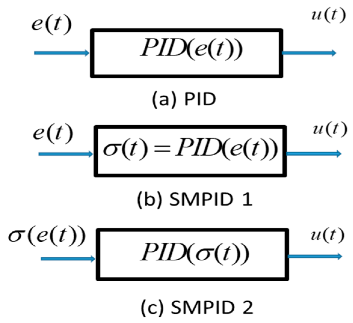
Figure 1. PID structures.
Axioms 12 00721 g001
Figure 2. Model-free U-control system.
Axioms 12 00721 g002
Figure 3. Functions of σ ˙ = ρ ( σ ) .
Axioms 12 00721 g003
Figure 4. Trajectories of SMC and MFSMC.
Axioms 12 00721 g004
Figure 5. Output response y ( t ) —SMPI.
Axioms 12 00721 g005
Figure 6. Control u ( t ) —SMPI.
Axioms 12 00721 g006
Figure 7. Error e ( t ) = r ( t ) y ( t ) —SMPI.
Axioms 12 00721 g007
Figure 8. Sliding mode function σ ( t ) —SMPI.
Axioms 12 00721 g008
Figure 9. States x 1 , x ^ 1 —SMPI.
Axioms 12 00721 g009
Figure 10. States x 2 , x ^ 2 —SMPI.
Axioms 12 00721 g010
Figure 11. Output response y ( t ) —SMNLP.
Axioms 12 00721 g011
Figure 12. Control u ( t ) —SMNLP.
Axioms 12 00721 g012
Figure 13. Error e ( t ) = r ( t ) y ( t ) —SMNLP.
Axioms 12 00721 g013
Figure 14. Sliding mode function σ ( t ) —SMNLP.
Axioms 12 00721 g014
Figure 15. States x 1 , x ^ 1 —SMNLP.
Axioms 12 00721 g015
Figure 16. States x 2 , x ^ 2 —SMNLP.
Axioms 12 00721 g016
Figure 17. Output response θ ( t ) —test 1.
Axioms 12 00721 g017
Figure 18. Control u ( t ) —test 1.
Axioms 12 00721 g018
Figure 19. e ( t ) = r ( t ) θ ( t ) —test 1.
Axioms 12 00721 g019
Figure 20. Output response θ ( t ) —test 2.
Axioms 12 00721 g020
Figure 21. Control u ( t ) —test 2.
Axioms 12 00721 g021
Figure 22. Error e ( t ) = r ( t ) θ ( t ) —test 2.
Axioms 12 00721 g022
Figure 23. System simulation (Simulink) block diagram.
Axioms 12 00721 g023
Figure 24. PID-CSMC—system output.
Axioms 12 00721 g024
Figure 25. PID-CSMC—control input.
Axioms 12 00721 g025
Figure 26. SMP—system output.
Axioms 12 00721 g026
Figure 27. SMP–control input.
Axioms 12 00721 g027
Figure 28. SMPI—system output.
Axioms 12 00721 g028
Figure 29. SMPI–control input.
Axioms 12 00721 g029
Disclaimer/Publisher’s Note: The statements, opinions and data contained in all publications are solely those of the individual author(s) and contributor(s) and not of MDPI and/or the editor(s). MDPI and/or the editor(s) disclaim responsibility for any injury to people or property resulting from any ideas, methods, instructions or products referred to in the content.