An Exploration and Exploitation-Based Metaheuristic Approach for University Course Timetabling Problems

Abstract

The university course timetable problem (UCTP) is known to be NP-hard, with solution complexity growing exponentially with the problem size. This paper introduces an algorithm that effectively tackles UCTPs by employing a combination of exploration and exploitation strategies. The algorithm comprises two main components. Firstly, it utilizes a genetic algorithm (GA) to explore the search space and discover a solution within the global optimum region. Secondly, it enhances the solution by exploiting the region using an iterated local search (ILS) algorithm. The algorithm is tested on two common variants of UCTP: the post-enrollment-based course timetable problem (PE-CTP) and the curriculum-based course timetable problem (CB-CTP). The computational results demonstrate that the proposed algorithm yields competitive outcomes when compared empirically against other existing algorithms. Furthermore, a t-test comparison with state-of-the-art algorithms is conducted. The experimental findings also highlight that the hybrid approach effectively overcomes the limitation of local optima, which is encountered when solely employing GA in conjunction with local search.

1. Introduction

Timetabling is an important and challenging area of research with diverse applications in education, enterprises, sports, transportation, human resources planning, and logistics. According to [1], timetabling refers to the allocation of given resources, subject to constraints, to objects placed in space–time, aiming to maximize the number of satisfied desirable objectives. These high-dimensional, multi-objective combinatorial optimization problems have received significant attention from the scientific community because manually generating timetables is laborious and time-consuming, often resulting in ineffective and costly schedules. Therefore, the development of automated timetabling systems is crucial to reducing errors, accelerating the creation process, and maximizing desirable objectives. Among the various forms of timetabling problems, the educational timetabling problem stands out as one of the most extensively studied. Finding a universal and effective solution for this problem is challenging due to its complexity, varying constraints, and evolving requirements.

The university course timetabling problem (UCTP) is a multidimensional assignment problem that involves assigning students and teachers to events (or courses), which are then allocated to appropriate timeslots and rooms. The UCTP can be categorized into two categories: post-enrollment-based course timetabling problems (PE-CTPs) and curriculum-based course timetabling problems (CB-CTPs). PE-CTP, sometimes referred to as “event timetabling”, focuses on assigning events to timeslots and resources (rooms and students) to avoid conflicts between events, timeslots, and rooms. The timetable is constructed after student enrollment to ensure all students can attend the events they are enrolled in. On the other hand, CB-CTP was first introduced in the Second International Timetabling Competition (ITC2007) [2] and is a weekly assignment problem that involves scheduling a specific number of lectures for various university courses within a given number of time periods and a set of rooms. Each day is divided into a fixed number of timeslots, and a period refers to a combination of a day and a timeslot. The total number of scheduling periods per week is determined by multiplying the number of days per week by the number of timeslots per day. Each course must be scheduled at different periods. Additionally, a set of curricula consists of groups of courses with shared students, and conflicts between courses are resolved based on the curricula rather than student enrollment data.

The main difference between these two variants of the UCTP is that in the PE-CTP, all objectives and constraints are based on the student’s enrollment in various course events, whereas in the CB-CTP, all objectives and constraints are associated with the curriculum conception, which is a set of courses that form a complete assignment for a group of students. An illustration of a student’s preference in the PE-CTP can be seen in the statement, “A student should have multiple events in a day.” Similarly, for the CB-CTP, a teacher’s preference can be exemplified by the statement, “A teacher prefers to have no more than two consecutive lectures.” These timetabling problems involve two types of constraints: hard and soft. Hard constraints are those that must be satisfied under any circumstances. A timetable is considered feasible if it successfully satisfies all hard constraints. On the other hand, soft constraints are more flexible and can be violated if necessary, but it is desirable to minimize these violations due to associated penalty costs. The lower the total value of the penalty cost, the higher the quality of the timetable. Thus, the main objective is to create a high-quality schedule with minimal penalties for violations of soft constraints.

Educational timetabling has been studied for over 60 years, beginning with Gotlieb [3]. Over the years, many solution approaches have been proposed by researchers. Carter et al. [4] provided an overview of the primary solution approaches for the UCTP and roughly divided them into four categories: constraint-based, sequential, clustered, and metaheuristic methods. In recent years, metaheuristic algorithms have been successfully applied for both variants of the UCTP and are classified into local area-based and population-based approaches. Local area-based algorithms, also called single-point algorithms, focus more on exploitation than exploration [5]. These algorithms work iteratively on a single solution and may not thoroughly explore the entire solution space. Examples of local area-based algorithms include tabu search (TS), iterated local search (ILS), very large neighborhood search (VLNS), and simulated annealing (SA). On the other hand, population-based algorithms, also known as multiple-point algorithms, are good at exploration rather than exploitation [6]. These algorithms maintain multiple solutions within a population and employ a selection process to update the solutions. They extensively search the entire solution space to find a globally optimal solution and are sometimes referred to as global area-based algorithms. Consequently, these algorithms do not focus solely on individuals with good fitness within a population but instead explore the entire solution space to identify potential solutions. However, premature convergence is the main disadvantage of such types of algorithms. Commonly utilized population-based algorithms for timetabling problems include the genetic algorithm (GA), artificial bee colony (ABC), particle swarm optimization (PSO), and ant colony optimization (ACO).

Driven by these discoveries and acknowledging that exploration, carried out through population-based algorithms, and exploitation, executed via local area-based algorithms, are two significant attributes of an optimization algorithm, which complement each other and necessitate fine-tuning between them, we propose a hybrid metaheuristic algorithm named GAILS, for solving PE-CTP and CB-CTP. The algorithm iteratively explores the search space, finds the global optimum region using GA, and then employs ILS to obtain the global optimum solution by exploiting this region. The GA generally fails to reach a global optimum because it repeatedly explores various sub-parts of the search space, leading to a long execution time. Additionally, the GA incorporates a local search (LS) which tends to become trapped in a local optimum quickly. Therefore, when dealing with a large search space, the GA might either fail to converge to a global optimum solution or require a significant amount of time due to the possibility of getting trapped in a local optimum. At this juncture, ILS is used to escape from the local optimum by applying perturbations to the current solution. This allows one to maintain a proper balance between the merits of these algorithms. Consequently, GA emphasizes exploration and diversification, while ILS concentrates on the exploitation and intensification of the search space. Various crossover and mutation operators, as well as neighborhood and perturbation moves, are utilized by the algorithm to generate new solutions.

The superiority of GAILS can be attributed to its hybridization of two complementary approaches. It initiates the search by using GA with an LS approach to explore the search space and identify the global optimum region, which is prone to becoming trapped in a local optimum. To overcome this challenge, ILS is employed, introducing perturbations to the current solution and facilitating escape from local optima. Furthermore, we conducted experimental investigations with varying time limits to demonstrate GAILS’ capability to evade local optima. The results affirm the effectiveness of our proposal, as the solution quality improves with increased time. Additionally, we evaluate the algorithm’s performance on benchmark problem instances of differing complexity, employing the fitness function value as a metric and comparing it with other algorithms using a t-test.

The structure of this paper is as follows: In Section 1, an introduction is provided. Section 2 contains a brief literature review of the related work on PE-CTP and CB-CTP. The PE-CTP and CB-CTP, along with their mathematical formulation, are explained in Section 3. Section 4 covers the description of the GAILS algorithm. Implementation and testing of GAILS on different benchmark problem instances with varying complexity are performed in Section 5. Finally, conclusions are summarized in Section 6.

2. Related Work

In different subsections of this section, the earlier research on the two UCTP versions, PE-CTP and CB-CTP, is discussed in detail.

2.1. Related Work on PE-CTP

The history of the educational scheduling problem can be traced back over six decades, starting with [3]. Over the years, numerous researchers have proposed different solution approaches and tested them on real-world problem instances. Despite significant progress in this field, researchers have faced difficulties when comparing their algorithms with existing state-of-the-art solutions due to differing problem formulations and instances used by each researcher. To address this issue, the International Metaheuristic Network organized the First International Timetabling Competition (ITC2002) in 2002. The objective was to simulate a realistic scenario where students have priorities when selecting events, and the timetable is constructed based on these preferences. Since then, these artificially generated enrollment-based course timetable problem instances have become the standard in the research community. Various researchers have utilized these instances to demonstrate the effectiveness of their novel techniques.

Socha et al. [7] utilized the same data generator to produce eleven instances of PE-CTP. They proposed the MAX-MIN ant system, which incorporates a local search routine optimized by creating an appropriate construction graph. The pheromone value determined the allocation of events to timeslots within specified bounds. The authors concluded that the MAX-MIN ant system outperformed random restart local search when applied to a set of typical problem instances. Rossi et al. [8] conducted a fair comparison of five different metaheuristic algorithms for solving the PE-CTP by using a common solution representation and standard neighborhood structure. Their empirical investigation revealed that each metaheuristic has distinct capabilities in satisfying hard and soft constraints, and an approach suitable for hard constraints may not be appropriate for optimizing soft constraints. Ref. [9] introduced a TS hyper-heuristic where heuristics compete to be selected by the hyper-heuristic.

Burke et al. [10] introduced an investigation into a simple, generic hyper-heuristic method for solving the PE-UCTP. They employed a set of widely used constructive heuristics, specifically graph coloring heuristics. The main characteristic of their method is to utilize a TS approach to alter the permutations of six graph coloring heuristics before creating a timetable. The outcomes of the approach improved further when a higher number of low-level heuristics were applied. In [11], an adaptive randomized descent algorithm (ARDA), which employs an adaptive criterion to escape from local optimal solutions, is described. Ref. [12] proposed a basic harmony search algorithm (BHSA) that takes advantage of the benefits of population-based algorithms by identifying the promising region in the search space using memory consideration and randomness. The proposed approach also used the benefits of local area-based algorithms by fine-tuning the search space region. They also introduced two modifications to the BHSA and proposed a modified harmony search algorithm (MHSA). The first modification involved considering memory, while the second modification aimed to enhance the functionality of the pitch adjustment operators by replacing the acceptance rule from a ‘random walk’ to a ‘first improvement’ and ‘side walk’ approach.

The approach by Cambazard et al. [13] for PE-CTP utilized constraint programming techniques and LS. They demonstrated the advantages of applying a list-coloring relaxation to the problem. They achieved the best constraint programming approach through various investigations and maintained the original problem decomposition. Additionally, they introduced lower bounds to estimate the costs related to the soft constraints in the problem. Motivated by the perception of a gravitational emulation local search algorithm, ref. [14] proposed a new population-based local search (PB-LS) heuristic for their solution. The authors integrated a multi-neighborhood particle collision algorithm and an adaptive randomized descent algorithm into their proposed approach, aiming to address the constraints of population-based algorithms. Ref. [15] proposed an integer linear programming-based heuristic to solve a real-world PE-CTP arising in an institution in Buenos Aires, Argentina. The algorithm produced high-quality results and provided generalizations to other related problems in the literature. Ref. [16] proposed a two-stage approach for solving the PE-CTP. The first phase focused on obtaining a feasible solution by satisfying all the hard constraints. In the second phase, they aimed to improve the solution quality by minimizing violations of soft constraints. To execute this two-phased approach, they employed an enhanced version of the SA with a reheating algorithm called simulated annealing with improved reheating and learning (SAIRL). Additionally, they introduced a reinforcement learning-based approach to establish an effective neighborhood structure for search operations.

Over the years, many hybrid approaches by hybridizing a local area-based algorithm within a population-based algorithm have gained much interest [17]. Such hybridization aims to achieve an equilibrium between exploration and exploitation of the search space to achieve the benefits of population-based and local area-based approaches. Ref. [18] proposed GA with a repair function and local search for solving PE-CTP. They presented a new repair function capable of transforming an unfeasible timetable into a feasible one. The local search algorithm was employed before the next generation to enhance timetable quality. A hybrid evolutionary algorithm employing hybridization between a memetic algorithm and a randomized iterative improvement local search was given by [19]. They reduced the exploration ability of the search space by excluding the crossover operator from the memetic algorithm. Ref. [20] suggested a guided search genetic algorithm (GSGA) consisting of a guided search strategy and a local search technique for their solution. The guided search strategy introduced offspring into the population based on a data structure that stores information extracted from previous competent individuals. Subsequently, the LS technique is employed to enhance the overall quality of individual outcomes. Ref. [21] further proposed an extended guided search genetic algorithm (EGSGA) by introducing a new local search strategy in addition to the original local search strategy used in GSGA.

Ref. [22] proposed a hybrid metaheuristic algorithm that combines an electromagnetic-like mechanism and the great deluge algorithm for solving both variants of UCTP. The electromagnetic-like mechanism is a population-based stochastic global optimization approach that simulates the attraction, physics, and repulsion of sample points in moving toward optimality. The great deluge algorithm is a local search strategy that allows the worst solutions to be accepted by an upper boundary. The dynamic force estimated from the attraction–repulsion mechanism is used as a declining rate to update the search procedure. Ref. [23] presented a hybrid metaheuristic approach that combines the great deluge and tabu search. They proposed their solution approach for both PE-CTP and CB-CTP. The algorithm is divided into two parts, construction and improvement, and four different neighborhood moves are employed. Ref. [24] proposed a new hybrid algorithm that combines GA with local search and uses events based on groupings of students. Ref. [25] proposed a solution for the PE-CTP that is motivated by particle swarm optimization and implemented in the basic artificial bee colony algorithm. The algorithm was hybridized with the great deluge algorithm to enhance local exploitation capabilities and improve global exploration quality. This approach achieved equilibrium by using a combination of these techniques. Ref. [26] developed a new hybrid method that combines genetic-based discrete particle swarm optimization with local search and tabu search approaches for solving the PE-CTP.

A hybrid approach based on the improved parallel GA and LS (IPGALS) is proposed to solve the PE-CTP by [27]. The GA is enhanced by incorporating LS. IPGALS adopts a timetable representation, guaranteeing the preservation of hard constraints. The proposed approach is run parallel to enhance the GA searching process due to various problem constraints. The algorithm was tested on benchmark PE-CTP problem instances, and the results were compared to other methods previously used to solve PE-CTP, and it was found to be very effective. Ref. [28] proposed a review paper regarding the most recent scientific approaches applied to the UCTP. The study demonstrates different methodologies researchers use to solve the problem based on when they were created and what data they used. The paper also discusses the challenges and opportunities while solving the UCTP. They have found that metaheuristic approaches are widely favored, with hybrid and hyper-heuristic approaches subsequently employed to achieve effective outcomes. They also observed that the most advanced techniques found in the scientific literature are not always used in the real world, probably because they are not adaptable enough.

2.2. Related Work on CB-CTP

After successfully organizing ITC2002, the research community in the field of timetabling organized the Second International Timetabling Competition (ITC2007) in 2007 [2]. During this event, they introduced three tracks for educational timetabling problems, with the third track focusing on curriculum-based course timetabling applied to Italian universities. For this track, several datasets were derived from real-world examples provided by the University of Udine. These datasets primarily emphasized lecturers’ preferences rather than students’, as is the case in PE-CTP.

By nature, CB-CTP is a highly constrained and complicated combinatorial optimization problem extensively studied by a large number of researchers [22,29,30,31,32,33]. They classified them first, along with their mathematical formulations, and then proposed several solutions approaches. In general, there is no known efficient deterministic polynomial-time algorithm for their solution, and they are solved by a variety of exact and heuristic approaches. Ref. [4] discussed their main solution approaches and roughly divided them into four categories: constraint-based, sequential, clustered, and generalized search (metaheuristics) methods. In constraint-based approaches [29,34], these problems are represented as constraint satisfaction problems (CSPs) and solved using CSP-solving approaches. Ref. [29] proposed to formulate the timetabling instance of CB-CTP as CSP instances and applied a general-purpose CSP solver to find solutions. The solver effectively handled weighted constraints using a hybrid algorithm combining tabu search and ILS. Ref. [35] introduced a constraint-based solver approach for CB-CTP that included multiple local search approaches working in three stages.

Ref. [31] proposed a two-stage integer linear programming (ILP) model for the solution of CB-CTP. The approach involves decomposing the problem into two stages, each represented by a distinct ILP model. In the first stage, the objective is to assign lectures to time periods, whereas the assignment of lectures to rooms is performed in the second stage by considering room stability. In the first stage, the assignment is performed without considering rooms, minimum working days, curriculum compactness, or minimizing penalties for room capacity. The representation of CB-CTPs as graphs is demonstrated in [36], where vertices and connections correspond to the lectures of courses and the constraints between them. Subsequently, graph coloring algorithms are employed to solve these CB-CTPs. Although this kind of approach (sequential heuristics) has demonstrated greater efficiency in small-sized problem instances, it seems ineffective in large-sized problem instances. Ref. [37] have proposed a satisfiability (SAT) model to solve a real-world CB-CTP at a Mexican university. Ref. [38] proposed a harmony search algorithm for the solution of CB-CTP. In the execution of their algorithm, the process of improvisation consists of memory consideration, random consideration, and pitch adjustment. A high-level object-oriented model called QuikFix has been proposed by [39] for the solution of CB-CTP. A repair-based heuristic is used in their approach, and certain structural constraints and significant neighborhood moves are applied in the problem domain’s search space.

Other extensively explored areas, such as the adaptive approaches, metaheuristics, multi-criteria, and case-based reasoning discussed by [40], are also used to solve these problems. In recent years, metaheuristic approaches and hybrid approaches have been extensively used to solve CB-CTP. These metaheuristic approaches are motivated by nature and apply nature-like processes to obtain optimal or near-optimal solutions. These approaches are generally categorized as local area-based (ILS, TS, SA, and VLNS) and population-based (GA, ACO, ABC, and PSO) algorithms. According to [41], an ABC algorithm has four phases: initialization, the employed bee phase, the onlooker bee phase, and the scout bee phase. Ref. [42] proposed a new swarm intelligence algorithm based on ABC to solve the CB-CTP. Their algorithm works in two phases. The first phase is used to obtain a feasible solution by satisfying all the hard constraints. In contrast, the second phase is used to satisfy as many soft constraints as possible without violating any hard constraints. Ref. [32] proposed an adaptive tabu search (ATS) algorithm for their solution by the hybridization of TS and ILS. The algorithm uses two neighborhood structures, namely SimpleSwap and KampeSwap, and a standard tabu list to prevent the cycling of previously visited solutions for both moves.

Ref. [30] proposed a two-phase approach for resolving the CB-CTP problem in their publication. The first phase involved utilizing a robust single-stage simulated annealing method for problem-solving, while in the second phase, an extensive and statistically sound methodology was designed and applied for the parameter tuning process. This resulted in a methodology that models the relationship between search method parameters and instance features, allowing for the parameters of unseen instances to be set through a simple inspection. In [43], the CB-CTP was modeled as a bi-criteria optimization problem with two objectives: a penalty function and a robustness metric. The problem was resolved using a hybrid multi-objective genetic algorithm that integrates hill climbing and simulated annealing algorithms with the standard GA approach to produce an accurate approximation of the Pareto-optimal front. Ref. [33] explored the use of generational construction hyper-heuristics for automating the process of low-level construction heuristic generation for CB-CTP. Two hyper-heuristics, an arithmetic hyper-heuristic for evolving arithmetic heuristics and a genetic algorithm hyper-heuristic made up of ten problem attributes for generating hierarchical heuristics, were implemented and applied to solve CB-CTP.

Ref. [44] presented an answer set programming-based approach, termed a teaspoon, for solving the CB-CTP. In this approach, the system first reads a CB-CTP instance of a standard input format and converts it into a set of answer set programming facts. These facts are then combined with the first-order encoding for CB-CTP solving, which any off-the-shelf ASP system can subsequently solve. Ref. [45] proposed a novel competition-guided multi-neighborhood local search (CMLS) algorithm for solving the CB-CTP. The proposed algorithm consists of three main contributions. First, it combines different neighborhoods uniquely by selecting only one at each iteration. This helps find a balance between finding many options and being efficient with time. Second, the algorithm uses two rules to determine the likelihood of selecting a neighborhood. Lastly, CMLS has a restart strategy where two different local search procedures are used and the best result is used as the starting point for the next search. An extensive and systematic review of the utilization of metaheuristic approaches used for UCTPs has been proposed by [46]. They thoroughly review, summarize, and categorize these approaches while introducing a classification for hybrid metaheuristic methods. Additionally, their study critically analyzes these methods’ advantages and limitations, highlighting the challenges, gaps, and potential areas for future research.

3. Problem Formulation

This section outlines the two variants of UCTPs, namely, the PE-CTP and the CB-CTP, and presents their mathematical formulations. The UCTP is a multi-dimensional assignment problem where students and teachers are assigned to events (or courses), which are then allocated to appropriate timeslots and rooms. In the subsequent subsections, we delve into the PE-CTP and CB-CTP individually.

3.1. Post-Enrollment Based Course Timetabling Problem

This section provides an explanation of the PE-CTP, along with its mathematical formulation. The PE-CTP is characterized as a multi-dimensional assignment problem wherein students select events, such as lectures, tutorials, and laboratories. These events must be allocated to a certain number of timeslots (9 per day for 5 days) and rooms, with the goal of minimizing constraint violation. Each student selects multiple events, and each room has a specific capacity and various features. The resolution to this problem entails assigning the events to suitable timeslots and rooms that fulfill the specified hard constraints, as described below.

• Each student can attend only one event at any given timeslot.
• Each event must be assigned to a room with enough seating capacity and all the necessary features.
• Each room can host only one event at a time.

When only hard constraints are present, the goal is to find a feasible solution. In addition, the following soft constraints are considered, the violation of which leads to a certain penalty for the PE-CTP solution.

• Scheduling an event at the last timeslot of the day should be avoided.
• A student should not have more than two events in consecutive timeslots daily.
• Having only one event a day is not recommended for a student.

Next, the mathematical formulation of the PE-CTP can be described. The PE-CTP involves a set $\mathrm{E}$ consisting of n events assigned to 45 timeslots (with 9 timeslots per day for 5 days). There is also a set $\mathrm{R}$ of m rooms with fixed seating capacity where these events occur. In addition, a set $\mathrm{S}$ includes p students who can choose any event from $\mathrm{E}$, and a set $\mathrm{F}$ contains q room features required for events in selected rooms. The following notations are used in the formulation of the problem.

• The set of events, denoted as $\mathrm{E}=\{e_1,e_2,\dots ,e_n\}$, consists of n events.
• The set of rooms, denoted as $\mathrm{R}=\{r_1,r_2,\dots ,r_m\}$, contains m rooms.
• The set of timeslots, denoted as $\mathrm{T}=\{t_1,t_2,\dots ,t_{45}\}$, includes 45 timeslots.
• The set of students, denoted as $\mathrm{S}=\{s_1,s_2,\dots ,s_p\}$, comprises p students.
• The set of rooming features, denoted as $\mathrm{F}=\{f_1,f_2,\dots ,f_q\}$, represents q rooming features.
• $r_i.capacity$ represents the capacity of room $r_i$.
• A matrix $\mathrm{RF}={\left[r{f}_{ij}\right]}_{m\times q}$, called a room-feature matrix and represents the feature possessed by the room. Here, $r{f}_{ij}=1$, if room $r_i$ is having feature $f_j$; otherwise, the value is zero.
• The decision variable $x_{ijkl}$ represents student $s_i$ attending the event $e_j$ in the timeslot $t_k$ and in the room $r_l$. It is defined for i ranging from 1 to p, j ranging from 1 to n, k ranging from 1 to 45, and l ranging from 1 to m.

  $$x_{ijkl}=\left\{\begin{array}{cc}1\hfill & \mathrm{if}\mathrm{the}\mathrm{combination}\mathrm{mentioned}\mathrm{above}\mathrm{is}\mathrm{valid},\hfill \\ 0\hfill & \mathrm{otherwise}.\hfill \end{array}\right.$$
• The decision variable $y_{ijk}$ represents an event $e_i$ that takes place in the room $r_j$ with feature $f_k$. It is defined for $1\le i\le n$, $1\le j\le m$, and $1\le k\le q$.

  $$y_{ijk}=\left\{\begin{array}{cc}1\hfill & \mathrm{if}\mathrm{the}\mathrm{combination}\mathrm{mentioned}\mathrm{above}\mathrm{is}\mathrm{valid},\hfill \\ 0\hfill & \mathrm{otherwise}.\hfill \end{array}\right.$$
• The decision variable $z_{ij}$ represents an event $e_i$ that takes place in timeslot $t_j$ and defined for $1\le i\le n,\mathrm{and}1\le j\le 45$.

  $$z_{ij}=\left\{\begin{array}{cc}1\hfill & \mathrm{if}\mathrm{the}\mathrm{combination}\mathrm{mentioned}\mathrm{above}\mathrm{is}\mathrm{valid},\hfill \\ 0\hfill & \mathrm{otherwise}.\hfill \end{array}\right.$$

Now, the mathematical formulation of hard constraints can be described as follows:

• Each student can attend only one event at any given timeslot.

  $$\begin{array}{c}\hfill \sum _{j=1}^n\sum _{l=1}^m{x}_{ijkl}\le 1,1\le i\le p;1\le k\le 45.\end{array}$$
• Each event must be assigned to a room with enough seating capacity and all the necessary features.

  $$\begin{array}{c}\hfill \sum _{i=1}^p{x}_{ijkl}\le r_l.capacity,1\le j\le n;1\le k\le 45;1\le l\le m;\mathrm{and}\\ \hfill y_{ijk}\le r{f}_{jk},1\le i\le n;1\le j\le m;1\le k\le q.\end{array}$$
• Each room can host only one event at a time.

  $$\begin{array}{c}\hfill \sum _{j=1}^n{x}_{ijkl}\le 1,1\le i\le p;1\le k\le 45;1\le l\le m.\end{array}$$

Similarly, the soft constraints can be formulated mathematically as follows:

• Scheduling an event at the last timeslot of the day should be avoided.

  $$\begin{array}{c}\hfill \sum _{i=1}^n{z}_{ij}=0,j=9,18,\dots ,45.\end{array}$$
• A student should not have more than two events in consecutive timeslots daily.

  $$\begin{array}{c}\hfill \sum _{j=1}^n\sum _{l=1}^m\sum _{k=a}^{a+2}{x}_{ijkl}\le 2,1\le i\le p;\\ \hfill a=1,2,\dots ,7,10,11,\dots ,16,\dots ,37,38,\dots ,43.\end{array}$$
• Having only one event a day is not recommended for a student.

  $$\begin{array}{c}\hfill \sum _{j=1}^n\sum _{l=1}^m\sum _{k=d}^{d+8}{x}_{ijkl}>1,1\le i\le p;d=1,10,19,28,37.\end{array}$$

The objective is to achieve an optimal solution for the PE-CTP by satisfying all the hard constraints and reducing the overall penalty cost of the soft constraint violations. Therefore, the objective function $f\left(I\right)$ for an individual solution I can be defined as

$$minf\left(I\right)=\gamma \times hcv\left(I\right)+scv\left(I\right),$$

where $hcv\left(I\right)$ and $scv\left(I\right)$ represent the counts of hard and soft constraint violations in solution I, and γ is a constant greater than the maximum potential violation of the soft constraints. To simplify the process, a direct solution representation is used, which involves an integer-valued ordered list of size $\left|\mathrm{E}\right|$, denoted as $a\left[i\right]$, where $1\le a\left[i\right]\le 45\mathrm{and}1\le i\le \left|\mathrm{E}\right|$. Each element $a\left[i\right]$ represents the timeslot for event $e_i$. The assignment of rooms is generated using a matching algorithm where a set of events appearing in a timeslot and a pre-processed list of rooms based on their sizes and features are used. A bipartite matching algorithm is employed to obtain a maximum cardinality matching between these two sets, which is determined by using a deterministic network flow algorithm as provided by [47]. The remaining unplaced events are assigned to the room with the fewest events, in order, until all events are assigned. Following these procedures, a similar integer-valued ordered list of size $\left|\mathrm{E}\right|$, say $b\left[i\right]$, where $1\le b\left[i\right]\le m\mathrm{and}1\le i\le \left|\mathrm{E}\right|$ is obtained for the event-room assignments. Here, m denotes the total number of rooms. In the case of a tie, the first room is selected. This process leads to a complete assignment of all the events to suitable rooms and timeslots.

3.2. Curriculum-Based Course Timetabling Problem

This subsection presents a description of the CB-CTP and its corresponding mathematical formulation. The CB-CTP refers to a weekly assignment problem that involves the allocation of lectures for multiple courses within a given number of periods and a set of rooms. The day is split into a fixed number of timeslots, and each period is identified as a combination of a day and a timeslot. The total number of scheduling periods per week is determined by multiplying the number of days per week by the number of timeslots per day. It is necessary to schedule each course at different periods, and a set of curricula comprises a group of courses with shared students. In case of conflicts between courses, the curricula are used to resolve the issue instead of relying on student enrollment data. A feasible timetable is one in which all lectures are scheduled within a period and a room while satisfying the following hard constraints.

• All lectures of a course must take place in distinct rooms and periods.
• Two lectures cannot occur in the same room during the same period.
• All lectures for courses taught by the same teacher or within the same curriculum must be scheduled during different time periods. This means that there should not be any overlap of students or teachers during any given period.
• No lectures for the course can be assigned to a period if the teacher of the course is unavailable for that period.

Also, a penalty is imposed on the timetable for each violation of any of the following soft constraints:

• The lecture room’s capacity should not be exceeded by the number of students attending the course.
• All lectures in a course should be scheduled in the same room. If this is not possible, the number of occupied rooms should be as low as possible.
• The lectures of a course should be spread over the given minimum number of days.
• A curriculum incurs a violation when a lecture is not adjacent to any other lecture of the same curriculum within the same day. This requirement ensures that the student’s schedule is as compact as possible.

The aim is to minimize the violation of soft constraints. The problem involves assigning $\mathrm{TNL}$ lectures from a set $\mathrm{C}$ of n courses to $w=u\times v$ periods. Here, v and u represent the number of timeslots per day and the number of days per week, respectively. Additionally, the problem involves a set $\mathrm{R}$ of m rooms with different capacities. Each course $c_i\in \mathrm{C}$ comprises $n{\mathcal{l}}_i$ lectures, each scheduled at a different period and assigned to a different room. The problem also includes a set Π of x curricula, where each curriculum is a group of courses with common students. The following notations are used to establish the mathematical formulation of CB-CTP.

• $\Pi =\{{\pi }_1,{\pi }_2,\dots ,{\pi }_x\}$ is a set of x curricula.
• $\mathrm{C}=\{c_1,c_2,\dots ,c_n\}$ is a set of n courses.
• $\mathrm{D}=\{d_1,d_2,\dots ,d_u\}$ is a set of u days in a week.
• $\mathrm{T}=\{t_1,t_2,\dots ,t_v\}$ is a set of v timeslots in a day.
• $\mathrm{P}=\{p_1,p_2,\dots ,p_w\}$ is a set of w periods, where $w=u\times v$.
• $\mathrm{R}=\{r_1,r_2,\dots ,r_m\}$ is a set of m rooms.
• $\mathrm{L}=\{{\mathcal{l}}_1,{\mathcal{l}}_2,\dots ,{\mathcal{l}}_{\mathrm{TNL}}\}$ is a set of $\mathrm{TNL}$ lectures.
• $n{\mathcal{l}}_i$ is the total number of lectures for course $c_i$. Taking $n{\mathcal{l}}_0=0$, a lecture ${\mathcal{l}}_k$ corresponds to a course $c_i$ for k satisfying ${\displaystyle \sum _{j=0}^{i-1}n{\mathcal{l}}_j<k\le \sum _{j=1}^{i}n{\mathcal{l}}_j,1\le i\le n}$. Also, ${\displaystyle \sum _{i=1}^{n}n{\mathcal{l}}_i=\mathrm{TNL}}$.
• $n{s}_i$ is the total number of students taking course $c_i$.
• $min{d}_i$ is the minimum number of days for course $c_i$.
• $r_i.capacity$ represents the capacity of room $r_i$.
• $X_{ijkl}$ is a decision variable representing that lecture ${\mathcal{l}}_i$ of course $c_j$ takes place in room $r_k$ at period $p_l$ and defined for $1\le i\le n{\mathcal{l}}_j,1\le j\le n,1\le k\le m,\mathrm{and}1\le l\le w$, as

  $$X_{ijkl}=\left\{\begin{array}{cc}1\hfill & \mathrm{if}\mathrm{the}\mathrm{combination}\mathrm{mentioned}\mathrm{above}\mathrm{is}\mathrm{valid},\hfill \\ 0\hfill & \mathrm{otherwise}.\hfill \end{array}\right.$$
• $Y_{ijk}$ is a decision variable representing that lecture ${\mathcal{l}}_i$ of course $c_j$ takes place at period $p_k$ and defined for $1\le i\le n{\mathcal{l}}_j,1\le j\le n,\mathrm{and}1\le k\le w$, as

  $$Y_{ijk}=\left\{\begin{array}{cc}1\hfill & \mathrm{if}\mathrm{the}\mathrm{combination}\mathrm{mentioned}\mathrm{above}\mathrm{is}\mathrm{valid},\hfill \\ 0\hfill & \mathrm{otherwise}.\hfill \end{array}\right.$$
• $Z_{ijk}$ is a decision variable representing that course $c_i$ takes place in room $r_j$ at period $p_k$ and defined for $1\le i\le n,1\le j\le m,\mathrm{and}1\le k\le w$, as

  $$Z_{ijk}=\left\{\begin{array}{cc}1\hfill & \mathrm{if}\mathrm{the}\mathrm{combination}\mathrm{mentioned}\mathrm{above}\mathrm{is}\mathrm{valid},\hfill \\ 0\hfill & \mathrm{otherwise}.\hfill \end{array}\right.$$
• ${\eta }_{ij}$ is a decision variable representing that course $c_i$ takes place in room $r_j$ and defined for $1\le i\le n$, and $1\le j\le m$, as

  $${\eta }_{ij}=\left\{\begin{array}{cc}1\hfill & \mathrm{if}\mathrm{the}\mathrm{combination}\mathrm{mentioned}\mathrm{above}\mathrm{is}\mathrm{valid},\hfill \\ 0\hfill & \mathrm{otherwise}.\hfill \end{array}\right.$$
• $un{a}_{ij}$ is a decision variable representing that course $c_i$ is unavailable at period $p_j$ and defined for $1\le i\le n,\mathrm{and}1\le j\le w$, as

  $$un{a}_{ij}=\left\{\begin{array}{cc}1\hfill & \mathrm{if}\mathrm{the}\mathrm{combination}\mathrm{mentioned}\mathrm{above}\mathrm{is}\mathrm{valid},\hfill \\ 0\hfill & \mathrm{otherwise}.\hfill \end{array}\right.$$
• ${\xi }_{ij}$ is a decision variable representing that course $c_i$ belongs to curriculum ${\pi }_j$ and defined for $1\le i\le n,\mathrm{and}1\le j\le x$, as

  $${\xi }_{ij}=\left\{\begin{array}{cc}1\hfill & \mathrm{if}\mathrm{the}\mathrm{combination}\mathrm{mentioned}\mathrm{above}\mathrm{is}\mathrm{valid},\hfill \\ 0\hfill & \mathrm{otherwise}.\hfill \end{array}\right.$$
• ${\mu }_{ij}$ is a decision variable representing that course $c_i$ takes place at period $p_j$ and defined for $1\le i\le n,\mathrm{and}1\le j\le w$, as

  $${\mu }_{ij}=\left\{\begin{array}{cc}1\hfill & \mathrm{if}\mathrm{the}\mathrm{combination}\mathrm{mentioned}\mathrm{above}\mathrm{is}\mathrm{valid},\hfill \\ 0\hfill & \mathrm{otherwise}.\hfill \end{array}\right.$$
• ${\rho }_{ij}$ is a decision variable representing that course $c_i$ takes place in day $d_j$ and defined for $1\le i\le n,\mathrm{and}1\le j\le u$, as

  $${\rho }_{ij}=\left\{\begin{array}{cc}1\hfill & \mathrm{if}\mathrm{the}\mathrm{combination}\mathrm{mentioned}\mathrm{above}\mathrm{is}\mathrm{valid},\hfill \\ 0\hfill & \mathrm{otherwise}.\hfill \end{array}\right.$$
• ${\tau }_{ij}$ is a decision variable representing that course of curriculum ${\pi }_i$ takes place at period $p_j$ and defined for $1\le i\le x,\mathrm{and}1\le j\le w$, as

  $${\tau }_{ij}=\left\{\begin{array}{cc}1\hfill & \mathrm{if}\mathrm{the}\mathrm{combination}\mathrm{mentioned}\mathrm{above}\mathrm{is}\mathrm{valid},\hfill \\ 0\hfill & \mathrm{otherwise}.\hfill \end{array}\right.$$

Now, the mathematical formulation of hard constraints can be described as follows:

• All lectures of a course must take place in distinct rooms and periods.

  $$\begin{array}{ccc}& & \sum _{i=1}^{n{\mathcal{l}}_j}{Y}_{ijk}\le 1,1\le j\le n;1\le k\le w;\hfill \\ & & \sum _{i=1}^{n{\mathcal{l}}_j}\sum _{k=1}^w{Y}_{ijk}=n{\mathcal{l}}_j,1\le j\le n.\hfill \end{array}$$
• Two lectures cannot occur in the same room during the same period.

  $$\begin{array}{c}\hfill \sum _{j=1}^n\sum _{i=1}^{n{\mathcal{l}}_j}{X}_{ijkl}\le 1,1\le k\le m;1\le l\le w.\end{array}$$
• All lectures for courses taught by the same teacher or within the same curriculum must be scheduled during different time periods. This means that there should not be any overlap of students or teachers during any given period.

  $$\begin{array}{c}\hfill \sum _{j=1}^n\sum _{i=1}^{n{\mathcal{l}}_j}\sum _{k=1}^m(X_{ijkl}\times {\xi }_{jy})\le 1,1\le l\le w;1\le y\le x.\end{array}$$
• No lectures for the course can be assigned to a period if the teacher of the course is unavailable for that period.

  $$\begin{array}{c}\hfill \sum _{i=1}^{n{\mathcal{l}}_j}{Y}_{ijk}\le 1-un{a}_{jk},1\le j\le n;1\le k\le w.\end{array}$$

Similarly, the soft constraints can be formulated mathematically as follows:

• The lecture room’s capacity should not be exceeded by the number of students attending the course.

  $$\begin{array}{c}\hfill {\eta }_{ij}\times n{s}_j\le r_j.capacity,1\le i\le n;1\le j\le m.\end{array}$$
• All lectures in a course should be scheduled in the same room. If this is not possible, the number of occupied rooms should be as low as possible.

  $$\begin{array}{c}\hfill \sum _{k=1}^w{Z}_{ijk}-w\times {\eta }_{ij}\le 0,1\le i\le n;1\le j\le m.\end{array}$$
• The lectures of a course should be spread over the given minimum number of days.

  $$\begin{array}{ccc}& & \sum _{j=1}^v{\mu }_{ij}-{\rho }_{ik}\ge 0,1\le i\le n;1\le k\le u;\mathrm{and}\hfill \\ & & \sum _{j=1}^u{\rho }_{ij}\ge min{d}_i-H_i,1\le i\le n.\hfill \end{array}$$
  Here, $H_i$ will take the value 0 if and only if course $c_i$ takes more than ($min{d}_i-1$) number of days.
• A curriculum incurs a violation when a lecture is not adjacent to any other lecture of the same curriculum within the same day. This requirement ensures that the student’s schedule is as compact as possible.

  $$\begin{array}{ccc}& & \sum _{i=1}^n({\mu }_{ij}\times {\xi }_{ik})-{\tau }_{kj}=0,1\le j\le w;1\le k\le x;\mathrm{and}\hfill \\ & & -{\tau }_{i(j-1)}+{\tau }_{ij}-{\tau }_{i(j+1)}-I_{ij}\le 0,1\le i\le x;1\le j\le w.\hfill \end{array}$$
  Here, ${\tau }_{i(j-1)}$ is removed for $j=1,\frac{w}{u}+1,2\times \frac{w}{u}+1,\dots ,(u-1)\times \frac{w}{u}+1$, and ${\tau }_{i(j+1)}$ is removed for $j=\frac{w}{u},2\times \frac{w}{u},\dots ,u\times \frac{w}{u}$. Also, $I_{ij}$ will take the value 1 if ${\pi }_i$ has an isolated lecture at period $p_j$.

Similar to the PE-CTP, the goal is to attain an optimal solution for the CB-CTP by satisfying all the hard constraints and minimizing the penalty cost of the soft constraint violations. Hence, the objective function $f\left(I\right)$ for an individual solution I can be defined as follows:

$$minf\left(I\right)=\gamma \times hcv\left(I\right)+scv\left(I\right),$$

where the symbols retain their usual meanings. Here also, a direct solution representation is selected. A solution involves an integer-valued ordered list of size $\mathrm{TNL}$, say $a\left[i\right](1\le a[i]\le |\mathrm{P}|\mathrm{and}1\le i\le \mathrm{TNL})$. Here, list $a\left[i\right]$ corresponds to the assigned periods. Taking $n{\mathcal{l}}_0=0$, the k consecutive entries of $a\left[i\right]$, satisfying ${\sum }_{j=0}^{i-1}n{\mathcal{l}}_j<k\le {\sum }_{j=1}^{i}n{\mathcal{l}}_j$ are corresponding to the periods for all the $n{\mathcal{l}}_i$ number of lectures of course $c_i$. Once the assignments of all the lectures for all the courses to periods are completed, the room assignments are made by using a bipartite matching algorithm. A set of courses appears in a period and a set of rooms based on their sizes. Now, a bipartite matching algorithm is used to obtain a maximum cardinality matching between these two sets using a deterministic network flow algorithm as given by [47]. This solves our CB-CTP by assigning all courses to the appropriate rooms and periods.

4. Proposed Hybrid Metaheuristic Approach

This section develops the proposed exploration and exploitation-based metaheuristic algorithm that combines GA and ILS to find an optimal solution for the UCTP.

The study conducted by Golberg [48] observed that although GAs can identify potential regions for global optima in the search space, they face significant challenges when dealing with highly constrained problems. Moreover, it has been noted [49,50] that hybridizing GA with other optimization techniques can yield even better solutions. Incorporating these findings, we propose an approach for finding optimal solutions for PE-CTP and CB-CTP. Our algorithm aims to reduce the exponential time complexity of GA by combining it with the ILS algorithm, thereby increasing the likelihood of convergence to an optimal solution in the search space. The ILS algorithm refines the GA search and improves the chances of convergence to an optimal solution through successive iterations in various sub-parts of the search space. It is important to note that while GA may generate individuals representing both good and bad search spaces, the ILS algorithm ensures fairness by exploring different sub-parts of the search space.

Let us briefly recall the basic concepts of GA to explain the technical details of our algorithm. This stochastic algorithm is based on the principle of survival of the fittest and is used to iteratively map a population of solutions, known as chromosomes with fitness values, into a new population of solutions known as offspring. It requires the problem-specific encoding of a solution, where genes on chromosomes are characterized by variables. Therefore, it works with a randomly generated population of solutions in the search space and consists of three primary processes: selection, reproduction, and replacement.

In the selection process, more duplications of candidate solutions with higher fitness function values are made to enforce the survival-of-the-fittest mechanism. The reproduction stage uses crossover and mutation operators for the selected parents. In the crossover, segments of two solutions in the population are combined to obtain new and possibly improved solutions. In contrast, a solution is modified locally in a random order in the mutation process. Finally, the original parental population is replaced by a population of offspring solutions generated through the selection and reproduction processes. This replacement includes keeping the best solutions and removing the worst ones. The selection phase ensures better utilization of healthier offspring, while the reproduction phase ensures adequate exploration of the search space. Natural selection ensures the propagation of better fitness function values on chromosomes in future generations. The algorithmic layout of GAILS can be found in Algorithm 1. The complete working procedure of GAILS is shown in the flow chart in Figure 1.

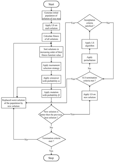
Figure 1. Flow chart of GAILS.

Remark 1. 

The algorithms and descriptions provided are designed based on PE-CTP. However, in the case of CB-CTP, the event $e_i\in E$ and timeslot $t_k\in T$ are replaced with lecture $l_i\in L$ and period $p_k\in P$, respectively, along with their respective parameters.

Algorithm 1  The proposed hybrid metaheuristic approach−GAILS
Require: A problem instance I
Ensure: an optimal solution $y_{\mathrm{best}}$ for I
1: begin
2: for $(i\leftarrow 1tomax)$ do	▹ randomly generated initial population of size $max$
3:     $y_i\leftarrow \mathrm{randomly}\mathrm{generated}\mathrm{starting}\mathrm{solution}$;
4:     $y_i\leftarrow \mathrm{solution}\mathrm{obtained}\mathrm{by}\mathrm{applying}\mathrm{LS}$;	▹ LS given in Algorithms 3 and 4
5:     compute fitness function value of $y_i$;
6: end for
7: organize the population of solutions in ascending order based on their fitness function values;
8: $y_{\mathrm{best}}\leftarrow y_1$;	▹$y_1$ denotes the finest solution within the population
9: repeat
10:     use tournament selection to select two parents from population;
11:     $y\leftarrow$ offspring solution obtained by applying crossover with α rate and mutation with β rate;
12:     if $(f\left(y\right)<f\left(y_{\mathrm{best}}\right))$ then	▹$f\left(y\right)$ is the fitness function value of y
13:         $y\leftarrow \mathrm{solution}\mathrm{generated}\mathrm{after}\mathrm{applying}\mathrm{ILS}\mathrm{to}y$;	▹ ILS given in Algorithm 2
14:     end if
15:     $y_{max}\leftarrow y$;	▹ the worst solution $y_{max}$ is replaced by y in the population of sorted solutions
16:     create and sort the population of solutions in ascending order of their fitness function values;
17:     $y_{\mathrm{best}}\leftarrow y_1$;
18: until (termination criteria not satisfied);
19: end

Since all the variables in both PE-CTP and CB-CTP problems are binary, there is no need for special methods for the solution encoding. Chromosomes in the proposed algorithm are vectors of Boolean values of all decision variables. For the PE-CTP problem: $y_i=(x_{1,1,1,1},\dots ,x_{p,n,45,m},y_{1,1,1},\dots ,y_{n,m,q},z_{1,1},\dots ,z_{n,45})$. For the CB-CTP problem: $y_i=(X_{1,1,1,1},\dots ,X_{n{\mathcal{l}}_n,n,m,w},Y_{1,1,1},\dots ,Y_{n,{\mathcal{l}}_n,w},Z_{1,1,1},\dots ,Z_{n,m,w},{\eta }_{1,1},\dots ,{\eta }_{n,m},un{a}_{i,j},\dots ,un{a}_{n,w},$${\xi }_{1,1},\dots ,{\xi }_{n,x},{\mu }_{1,1},\dots ,{\mu }_{n,w},{\rho }_{1,1},\dots ,{\rho }_{n,u})$.

By utilizing a uniform distribution, our proposed algorithm produces a population of random solutions with a size of $max$, where each event is assigned a timeslot. As the quality of the initial solutions impacts the final solutions, good initial solutions produce better results in less computation time [51,52]. We applied the LS to each initial population to create a population of good-quality initial solutions. The problem-specified heuristic information from the LS is then used by a steady-state evolution process in which only one pair of parent individuals is chosen for reproduction in each generation. The LS assigns events to timeslots and then uses the matching algorithm to allocate rooms to each event–timeslot pair using three neighborhood operators. Following that, the population of solutions is arranged in ascending order according to their fitness function values, where $y_1$ represents the best solution. Some individuals with the best fitness function values are randomly selected as parents from the current population. The fitness function $f\left(I\right)$ for an individual solution I is given by

$$f\left(I\right)=\gamma \times hcv\left(I\right)+scv\left(I\right),$$

where $hcv\left(I\right),scv\left(I\right),$ and γ are the counts of violations of hard and soft constraints on I, and a constant greater than the maximum possible violation of soft constraints, respectively. A child solution is generated using a uniform crossover operator with α probability and a mutation operator with β probability over the selected parents. Two individual solutions are chosen from the current population as the parents, using tournament selection with a suitable tournament size to create a child solution using a crossover operator. In our case, for each event, we select the parent with the smaller penalty value and assign their corresponding timeslot and room to the event of the child solution. Finally, a mutation operator is applied to the child solution obtained from the crossover operator.

The mutation operator is defined as a random move in the neighborhood of LS, which is extended with four-cycle permutations of the timeslots corresponding to four different events to complete the neighborhood of LS. Thus, the entire neighborhood consists of four categories of neighborhood moves. In a type 1 move, a random event from a timeslot is selected and moved to another timeslot. A type 2 move involves swapping two randomly chosen events between two different timeslots. A type 3 move selects two timeslots randomly and swaps all the events between them. Lastly, in a type 4 move, three randomly selected events from three different timeslots are permuted in one of the two possible ways.

A new solution y is obtained by applying the crossover and mutation operators on the selected parents using tournament selection. If $f\left(y\right)$ is less than $f\left(y_{\mathrm{best}}\right)$, the ILS algorithm described in Section 4.1 is applied to y. Here, $y_{\mathrm{best}}$ and $f\left(y_{\mathrm{best}}\right)$ correspond to the best solution in the population and the fitness function of the best solution, respectively. Next, the worst solution $y_{max}$ is replaced by the new solution y. The population of solutions is then sorted in increasing order of their fitness function values so that $y_1$ will be the best solution. This procedure is repeated until a termination criterion is met. Termination criteria may include a time limit, a number of iterations, or achieving an optimal solution with a zero fitness function value. The next subsection discusses the ILS and LS algorithms utilized in the GAILS.

4.1. Iterated Local Search Algorithm

This subsection describes, in brief, the ILS algorithm applied to solve the UCTP. The main disadvantage of LS is that it can become trapped in locally optimal solutions, which are considerably worse than the global optimal solution. It improves the LS algorithm by providing new starting solutions obtained from the current solution using perturbations rather than considering a random restart. Hence, ILS escapes from the local optimal solution by using perturbations. Every single execution of a perturbation in it creates a new solution. The strength of the perturbation is defined as the number of solution components that are modified. It is crucial that the LS algorithm cannot undo the perturbation, or else the solution will fall back into the just-visited local optimal solution. To apply ILS, four components are specified. The first component, “GenerateInitialSolution”, modifies y in GAILS to generate the initial solution $y_0$, which is further improved to a new solution y by applying LS. The second component, “Perturbation”, enhances the quality of the current solution y by taking it to some intermediate solution $y^{\prime }$. The third component, “LocalSearch”, takes solution $y^{\prime }$ and gives an enhanced solution $y^{″}$. Finally, the fourth component, “AcceptanceCriteria”, selects the solution for the next perturbation, with the acceptance criteria requiring the cost to decrease.

The article ref. [53] proposed that executing a random move within a higher-order neighborhood is more effective for achieving excellent performance in perturbation than moves performed in the LS algorithm. The perturbations should be compatible with the LS algorithm and consider the problem’s properties for better results. If the perturbation is too strong, the ILS algorithm may function similarly to a random restart. Conversely, if the perturbation is too small, the LS algorithm will likely return to the previously visited local optimal solution, limiting the diversification of the search space. The solution returned by the AcceptanceCriteria employs this perturbation. The ILS algorithm is described in Algorithm 2.

Algorithm 2  Iterated local search algorithm−ILS

Require:  A solution $y_0$ from the population Ensure:  An enhanced solution y 1: begin 2: $y_0\leftarrow \mathrm{GenerateInitialSolution}\left(\right)$; 3: $y\leftarrow \mathrm{apply}\mathrm{LS}\mathrm{with}{y}_0$; 4: while (termination criteria not met) do 5:     $y^{\prime }\leftarrow \mathrm{Perturbation}(y,\mathrm{History})$; 6:     $y^{″}\leftarrow \mathrm{apply}\mathrm{LocalSearch}\mathrm{with}{y}^{\prime }$; 7:     $y\leftarrow \mathrm{AcceptanceCriteria}(y,y^{″},\mathrm{History})$; 8: end while 9: end

The ILS method is utilized by starting with the randomly generated initial solution $y_0$ of PE-CTP. The LS algorithm is applied to $y_0$ with the help of some designed neighborhoods to obtain an enhanced solution y. The new solution y is then subjected to perturbation to obtain a further improved solution $y^{\prime }$. The perturbation employs the search history, referred to as History, to mine the previously discovered local optima, which are used to generate better starting points for LS. After that, LS is applied once more to $y^{\prime }$ to obtain a further improved solution $y^{″}$. If the solution $y^{″}$ satisfies the acceptance criteria based on the specified History, it replaces $y^{\prime }$. The ILS method is repeated until the predefined termination criteria used in GAILS are met. In our study, we utilize the following four types of perturbation moves:

Per₁: 

Selecting a different timeslot to a randomly chosen event.

Per₂: 

Swapping timeslots for two randomly chosen events.

Per₃: 

Selecting two timeslots randomly and swapping all their events.

Per₄: 

Selecting three events randomly and permuting them into three distinct timeslots in one of the two possible ways that differ from the existing one.

The random choices mentioned above were selected from a uniform distribution. To determine the strength of the perturbation, each individual random move is performed r times, where $r\in \{1,5,10,20,40,50,100\}$. We have considered three different methods to accept solutions in the AcceptanceCriteria. The initial method, Random_Walk, consistently accepts the new solution $y^{″}$ that LS returns. The second method, Accept_if_Better, only accepts a new solution $y^{″}$ if it is an improvement over the current solution y. The third method is Simulated_Annealing, which accepts $y^{″}$ if it is superior to the current solution; otherwise, it is accepted with a probability determined by $g\left(y\right)$. Here, $g\left(y\right)$ represents the total count of $hcv$ or $scv$, depending on whether solutions y and $y^{″}$ are feasible. Two methods used for calculating this probability are

M₁: 

${\mathrm{Prob}}_1(y,y^{″})=e^{-\frac{(g\left(y\right)-g\left(y^{″}\right))}{T}}$

M₂: 

${\mathrm{Prob}}_2(y,y^{″})=e^{-\frac{(g\left(y\right)-g\left(y^{″}\right))}{T.g\left(y_{\mathrm{best}}\right)}}$

Here, T and $y_{\mathrm{best}}$ represent a temperature parameter and the optimal solution obtained so far. Throughout the execution, the value of T remains constant. Generally, the temperature decreases over time in the SA algorithm to facilitate convergence towards a local minimum. However, when the ILS algorithm incorporates SA, the temperature is maintained at a constant level. The reason is that the ILS algorithm employs a distinct strategy to overcome local minima. Instead of reducing the temperature, the ILS algorithm introduces perturbations to alter the solution randomly. This allows the algorithm to explore new regions of the search space and potentially escape from local minima. Further, the value of T are selected from $\{0.01,0.1,1\}$ and $\{0.05,0.025,0.01\}$ for ${\mathrm{M}}_1$ and ${\mathrm{M}}_2$, respectively.

4.2. Local Search Algorithm

The classical method of local search is often used to find optimal solutions for many combinatorial optimization problems through two phases. The first phase is called the construction phase, which establishes feasibility. The second phase, the improvement phase, optimizes soft constraints without violating the feasibility of the search space. During the construction phase, the algorithm commences with an empty timetable and systematically builds up a schedule by gradually including one event at a time. Typically, the initial timetable is of poor quality with numerous constraint violations. The improvement phase then gradually enhances the timetable’s quality by modifying certain events to achieve a better timetable. The selection of good neighborhoods is a critical aspect of LS.

To solve PE-CTP, the construction and improvement phases of LS are applied to each individual solution. During the construction phase, all possible neighborhood moves are attempted for each event from the list of events associated with $hcv$ and ignoring all $scv$ until a termination criterion is reached. Termination criteria can be an improvement in the solution or the exhaustion of the pre-specified number of iterations. For simplicity, a portion of the given solution is customized to form a new neighboring solution. In this work, we used a neighborhood consisting of three smaller neighborhoods, ${\mathrm{N}}_1,{\mathrm{N}}_2,$ and ${\mathrm{N}}_3$, defined as follows:

N₁: 

An operator that randomly chooses a single event and moves this event to a different timeslot that produces the lowest penalty.

N₂: 

An operator that swaps the timeslots of two randomly selected events.

N₃: 

An operator that randomly selects two timeslots and swaps all their events.

The neighborhood operator ${\mathrm{N}}_2$ is applied only when ${\mathrm{N}}_1$ fails, and ${\mathrm{N}}_3$ is applied only when both ${\mathrm{N}}_1$ and ${\mathrm{N}}_2$ fail. In this context, the term “penalty” refers to the number of violations of hard and soft constraints. The resulting disturbance in room allocation is resolved by applying the bipartite graph matching algorithm to the affected timeslots after each neighborhood move, using its delta-evaluated measure. Delta-evaluation refers to the computation of the $hcv$ of events that move within a solution to obtain the fitness function value dispute between the related event’s pre- and post-move. If there are no new moves in the neighborhood or the current event has no $hcv$, the construction phase proceeds to the next event. If there is any remaining $hcv$ after applying all neighborhood moves to all events, the construction phase ceases to function without discovering a viable solution to the problem. Once a feasible solution is achieved, the improvement phase begins. It operates similarly to the construction phase but focuses on satisfying soft constraints instead of hard constraints. The goal is to minimize the $scv$ by applying all neighborhood moves to each event in sequential order without violating hard constraints. In summary, the construction phase provides a feasible solution, while the improvement phase aims to optimize the solution by satisfying as many soft constraints as possible. Algorithms 3 and 4 illustrate the general framework of the LS algorithm in its construction and improvement phases.

Algorithm 3  Construction phase of the local search algorithm
Require: A solution I from the population
Ensure: Either a feasible solution I or the nonexistence of a viable solution
1: begin
2: construct a randomly ordered circular list $(e_1,e_2,\dots ,e_n)$ consisting of n events;
3: $i\leftarrow 0$;	▹i is the event counter
4: select event $e_i$ after $i\leftarrow i+1$;	▹ move to the next event
5: if (all neighborhood moves applied to all the events) then
6:     if (∃ any $hcv$ in I) then
7:         END LOCAL SEARCH;
8:     else
9:         output a feasible solution I and END the construction phase;
10:     end if
11: end if
12: if ((feasible $e_i$) ⋁ (no untried move left for $e_i$)) then
13:     goto 4;
14: end if
15: $CheckSolution(e_i,I)$;	▹ all neighborhood moves applied and return the solution I
16: if (reduced number of $hcv$ in I) then
17:     make the move;
18:     goto 3;
19: else
20:     goto 12;
21: end if
22: end

Algorithm 4 Improvement phase of the local search algorithm
Require: Solution I from Algorithm 3
Ensure: An optimal solution I
1: begin
2: use the circular randomly ordered list $(e_1,e_2,\dots ,e_n)$ of n events generated in Algorithm 3;
3: $i\leftarrow 0$;	▹i is the event counter
4: select event $e_i$ after $i\leftarrow i+1$;	▹ move to the next event
5: if (all neighborhood moves applied to all the events) then
6:     END LOCAL SEARCH with an optimal solution I;
7: end if
8: if (($e_i$ NOT involved in any $scv$) ⋁ (no untried move left for $e_i$)) then
9:     goto 4;
10: end if
11: $CheckSolution(e_i,I)$;	▹ all neighborhood moves applied and return the solution I
12: if (number of $scv$ reduced in I without making I infeasible) then
13:     make the move;
14:     goto 3;
15: else
16:     goto 8;
17: end if
18: end

Procedure  $CheckSolution(e_i,I)$

$e_i$ and I are arguments. Returns I after neighborhood moves Require:  $\mathrm{T}$: the set of 45 timeslots; $\mathrm{R}$: the set of m rooms; 1: begin 2: apply ${\mathrm{N}}_1$ to solution I; 3: if (${\mathrm{N}}_1$ successful) then 4:     generate solution I; 5: else if (${\mathrm{N}}_1$ to I not successful) ⋀ (${\mathrm{N}}_2$ to I successful) then 6:     apply ${\mathrm{N}}_2$ to I and generate solution I; 7: else 8:     apply ${\mathrm{N}}_3$ to I and generate solution I; 9: end if 10: for$(k\leftarrow 1to45)$do 11:     if timeslot $t_k$ is effected by either of the move ${\mathrm{N}}_1$, ${\mathrm{N}}_2$, or ${\mathrm{N}}_3$ then 12:         use the matching algorithm for events held in $t_k$ to allocate rooms; 13:     end if 14: end for 15: delta-evaluate the result of the move; 16: return I; 17: end

5. Computational Results

In this section, we perform an experimental investigation to assess the performance of our proposed approach, GAILS, compared to several existing algorithms commonly used for solving the UCTP. The fitness function is employed as the measure of performance in all cases. We implemented all algorithms in GNU C++ version 4.5.2 and executed them on a PC with a processing speed of 3.10 GHz and 2 GB of RAM. We conducted experiments using two distinct sets of benchmark problem instances. The first set consists of 11 PE-CTP instances sourced from Socha’s benchmark dataset [7]. The second set includes 21 CB-CTP instances from the third track of ITC2007 (UD2). In the following subsections, we address these different problem instances separately.

5.1. Experiments on Socha’s Benchmark Dataset

In this subsection, the GAILS algorithm is tested over the 11 problem instances proposed by [7]. The given problem instances comprise a range of 100–400 events. These events must be organized within a timetable that covers 9 timeslots per day for 5 days. Ensuring that the scheduling satisfies both room capacity and room feature constraints is crucial. These instances are divided into five small instances, five medium instances, and one large instance. The parameter values and the detailed description of these problem instances have been presented in Table 1 and Table 2.

Table 1. Parameter values for the problem instances of [7].

Class	Small	Medium	Large
Number of events	100	400	400
Number of rooms	5	10	10
Number of students	80	200	400
Number of features	5	5	10
Approximate features per room	3	3	5
Percentage feature use	70	80	90
Maximum events per student	20	20	20
Maximum students per event	20	50	100

Table 2. Description of the problem instances of [7].

Instance	n	m	q	p	Max $\mathit{S}/\mathit{E}$	Max $\mathit{E}/\mathit{S}$	Avg. $\mathit{F}/\mathit{R}$	Avg. $\mathit{F}/\mathit{E}$
small01	100	5	5	80	15	15	$2.8$	$1.88$
small02	100	5	5	80	13	17	$3.0$	$2.02$
small03	100	5	5	80	20	13	$3.0$	$2.21$
small04	100	5	5	80	12	12	$4.4$	$2.92$
small05	100	5	5	80	17	19	$3.8$	$2.80$
medium01	400	10	5	200	11	20	$2.9$	$2.355$
medium02	400	10	5	200	11	20	$3.0$	$2.33$
medium03	400	10	5	200	12	20	$3.2$	$2.525$
medium04	400	10	5	200	11	20	$3.1$	$2.493$
medium05	400	10	5	200	20	20	$3.2$	$2.535$
large	400	10	10	400	30	20	$4.8$	$4.37$

$S/E$: students per event; $E/S$: events per student; $F/R$: features per room; $F/E$: features per event.

The GAILS algorithm is primarily executed on these problem instances, and the best combination of parameters is identified. The population size (δ), tournament size (ω), crossover probability (α), and mutation probability (β) are selected as $10,5,0.8,$ and $0.5$, respectively. The different parameters are selected for the ILS depending on the size of the problem instance. For small problem instances, ${\mathrm{Per}}_1$ with $r=1$ and ${\mathrm{M}}_2$ with $T=0.025$ are used. For medium and large problem instances, ${\mathrm{Per}}_1$ with $r=5$ and ${\mathrm{M}}_1$ with $T=0.1$ are used. The value of γ in the fitness function is set to ${10}^6$, which indicates that any solution I with $f\left(I\right)\ge {10}^6$ is infeasible.

To evaluate performance, all small problem instances are run independently for 100 trials, with a specific time-bound in each trial. The lowest fitness function value among them is used as the optimal solution’s performance measure. For medium and large problem instances, the trials are fixed at 50 and 20, respectively. The maximum number of iterations in LS is set to 200, 10,000, and 100,000, respectively. Initially, the time limit for all small problem instances is fixed at 2 s.

In Table 3, the results obtained for small problem instances are presented, showcasing the fitness function values of the best solution ($f_{\min }$), the worst solution ($f_{\max }$), and the time taken to achieve the best solution (Time). Notably, in each independent trial, the GAILS algorithm consistently produces the best solution with a fitness value of zero for all small problem instances. The graph in Figure 2 illustrates the relationship between the fitness function values and the time GAILS takes for these small problem instances. It is worth noting that the optimal solution is consistently achieved in a mere 0.2 s.

Table 3. Performance of small problem instances.

Instance	${\mathit{f}}_{\mathbf{min}}$	${\mathit{f}}_{\mathbf{max}}$	Time
small01	0	0	$0.052$
small02	0	0	$0.016$
small03	0	0	$0.008$
small04	0	0	$0.152$
small05	0	0	$0.020$

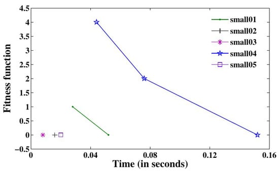
Figure 2. $f_{\min }$ versus time for small problem instances.

One of the goals of GAILS is to prevent local optima by incorporating perturbation within ILS. To support our claim, we executed medium problem instances under four different time limits: 900, 1200, 1500, and 12,000 s. This was chosen to examine how time duration affects the solution quality. In Table 4, Table 5, Table 6 and Table 7, we present the minimum ($f_{\min }$), maximum ($f_{\max }$), and average ($f_{\mathrm{avg}}$) fitness function values for all trials, along with the standard deviation (ς) and the corresponding time duration. The results demonstrate a significant improvement in fitness function values as the time limit increases. Figure 3 illustrates the best fitness function value attained by GAILS across all medium-sized problem instances for the four time periods. Each instance underwent independent testing for 20 trials, with a time limit of 12,000 s.

Table 4. Performance of medium problem instances with a time limit of 900 s.

Instance	${\mathit{f}}_{\mathbf{min}}$	${\mathit{f}}_{\mathbf{max}}$	${\mathit{f}}_{\mathbf{avg}}$	ς	Time
medium01	92	112	$102.23$	$5.538$	$818.14$
medium02	82	120	$99.13$	$9.958$	$803.51$
medium03	122	159	$139.77$	$12.42$	$857.35$
medium04	73	106	$90.37$	$9.397$	$641.20$
medium05	89	128	$109.90$	$12.14$	$871.69$

Table 5. Performance of medium problem instances with a time limit of 1200 s.

Instance	${\mathit{f}}_{\mathbf{min}}$	${\mathit{f}}_{\mathbf{max}}$	${\mathit{f}}_{\mathbf{avg}}$	ς	Time
medium01	85	111	$98.43$	$7.234$	$1097.41$
medium02	78	118	$98.73$	$10.65$	$1041.31$
medium03	112	159	$136.87$	$16.37$	$1198.55$
medium04	69	107	$85.97$	$9.995$	$1142.16$
medium05	77	124	$106.23$	$12.54$	$1152.59$

Table 6. Performance of medium problem instances with a time limit of 1500 s.

Instance	${\mathit{f}}_{\mathbf{min}}$	${\mathit{f}}_{\mathbf{max}}$	${\mathit{f}}_{\mathbf{avg}}$	ς	Time
medium01	78	111	$96.50$	$8.784$	$1482.74$
medium02	75	109	$91.27$	$10.02$	$1433.71$
medium03	102	159	$124.17$	$17.82$	$1452.59$
medium04	60	104	$81.97$	$11.70$	$1443.61$
medium05	70	128	$103.70$	$13.30$	$1478.37$

Table 7. Performance of medium problem instances with a time limit of 12,000 s.

Instance	${\mathit{f}}_{\mathbf{min}}$	${\mathit{f}}_{\mathbf{max}}$	${\mathit{f}}_{\mathbf{avg}}$	ς	Time
medium01	35	52	$42.05$	$5.395$	11,755.91
medium02	31	60	$40.85$	$8.362$	$9893.19$
medium03	56	83	$68.25$	$9.453$	11,638.80
medium04	35	57	$44.05$	$7.052$	11,809.90
medium05	43	66	$52.30$	$8.417$	11,498.91

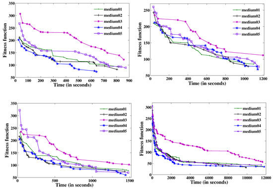
Figure 3. $f_{\min }$ versus time for medium problem instances with different time ranges.

Similarly, the large problem instance is executed over three different time limits, taken as 9000, 12,000, and 15,000 s, and $f_{\min },f_{\max },f_{\mathrm{avg}},\varsigma ,$ and time are obtained. These outcomes are presented in Table 8, Table 9 and Table 10. The best fitness function value versus time obtained by GAILS for the large problem instance over these different time limits is depicted by the graphs in Figure 4.

Table 8. Performance of large problem instance with a time limit of 9000 s.

Instance	${\mathit{f}}_{\mathbf{min}}$	${\mathit{f}}_{\mathbf{max}}$	${\mathit{f}}_{\mathbf{avg}}$	ς	Time (in Seconds)
large	585	708	635.35	40.24	8392.23

Table 9. Performance of large problem instance with a time limit of 12,000 s.

Instance	${\mathit{f}}_{\mathbf{min}}$	${\mathit{f}}_{\mathbf{max}}$	${\mathit{f}}_{\mathbf{avg}}$	ς	Time (in Seconds)
large	580	702	$614.95$	$36.27$	11,839.19

Table 10. Performance of large problem instance with a time limit of 15,000 s.

Instance	${\mathit{f}}_{\mathbf{min}}$	${\mathit{f}}_{\mathbf{max}}$	${\mathit{f}}_{\mathbf{avg}}$	ς	Time (in Seconds)
large	572	702	$612.6$	$38.50$	14,133.13

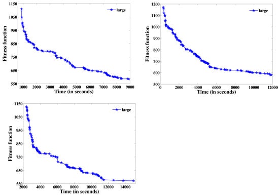
Figure 4. $f_{\min }$ versus time for large problem instance with different time ranges.

Figure 5 and Figure 6 depict boxplots that summarize the outcomes obtained from the medium and large problem instances across various time limits during all the independent trials. The boxplots represent the interquartile range, which is the span between the $25\%$ and $75\%$ quantiles of the data. A bar represents a median, while outliers are indicated using a plus sign.

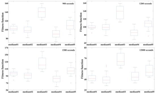
Figure 5. Boxplots of results obtained for medium-sized problems with various time limits.

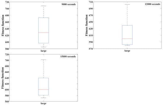
Figure 6. Boxplots of results obtained for large problem instances with various time limits.

5.1.1. Comparative Experiments

In this section, we initially compare the performance of GAILS with ILS, GALS, and NHA [24], as well as the existing algorithms GSGA [20], EGSGA [21], BHSA and MHSA [12]. To ensure a fair comparison, we maintain the same relevant parameters for GALS and ILS as those used in GAILS. For small-sized problem instances, we independently run all algorithms for $100,50,50,$ and 50 trials for GAILS, GALS, ILS, and NHA, respectively. For medium and large-sized problem instances, we independently run GALS and ILS for 50 trials each, while for NHA, this number is limited to 20. Similarly, for GAILS, the figure is 50 for medium-sized problems and 20 for large ones. We restrict the time limit to 2, 900, and 9000 s for small, medium, and large problem instances, respectively, for all algorithms.

We present the comparison of GAILS with GALS, ILS, and NHA through the graphs in Figure 7. The x-axis represents time in seconds, while the y-axis represents the best fitness function value. We give the results obtained by all eight algorithms for all problem instances in terms of $f_{\min },f_{\max },f_{\mathrm{avg}},$ and ς in Table 11. The term $x\%$ Inf. represents the percentage of infeasible solutions over all runs. The comparison results of Figure 7 and Table 11 show that GAILS is more effective than other algorithms, producing lower $f_{\mathrm{avg}}$ and ς on most problem instances. In fact, in some cases, the $f_{\max }$ obtained by GAILS is better than the $f_{\min }$ obtained by other algorithms. These results indicate that GAILS is more reliable than the other algorithms.

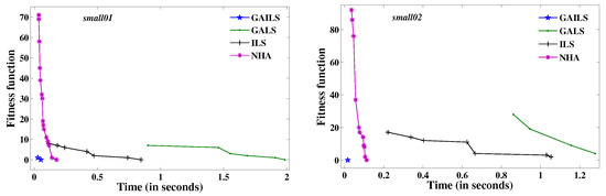
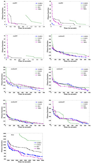
Figure 7. Comparison between GAILS, GALS, ILS, and NHA.

Table 11. Comparison of different algorithms on PE-CTP instances.

Instance		GAILS	GALS	ILS	NHA	GSGA	EGSGA	BHSA	MHSA
small01	$f_{\min }$	0	0	0	0	0	0	3	0
	$f_{\max }$	0	15	17	0	9	4	8	4
	$f_{\mathrm{avg}}$	0	8	$7.14$	0	$2.11$	$1.71$	5	$2.5$
	ς	0	$3.207$	$3.807$	0	$3.33$	$2.42$	$1.632$	$1.178$
small02	$f_{\min }$	0	4	2	0	0	0	4	0
	$f_{\max }$	0	21	20	0	16	11	9	4
	$f_{\mathrm{avg}}$	0	$11.78$	$10.32$	0	$2.32$	$2.01$	$6.3$	$2.5$
	ς	0	$4.117$	$3.857$	0	$5.59$	$3.71$	$1.494$	$1.269$
small03	$f_{\min }$	0	2	0	0	0	0	2	0
	$f_{\max }$	0	17	21	0	11	2	5	2
	$f_{\mathrm{avg}}$	0	$8.98$	$8.76$	0	$2.2$	$1.8$	$3.7$	$0.8$
	ς	0	$3.583$	$4.547$	0	$3.21$	$1.53$	$1.059$	$0.788$
small04	$f_{\min }$	0	1	0	0	0	0	3	0
	$f_{\max }$	0	14	19	0	11	5	5	3
	$f_{\mathrm{avg}}$	0	$7.48$	$7.58$	0	$1.84$	$0.63$	$3.4$	$1.2$
	ς	0	$2.808$	$4.366$	0	$2.20$	$1.89$	$0.843$	$0.918$
small05	$f_{\min }$	0	0	0	0	0	0	1	0
	$f_{\max }$	0	12	14	0	5	3	4	0
	$f_{\mathrm{avg}}$	0	$5.5$	$4.12$	0	$0.51$	$0.55$	$2.8$	0
	ς	0	$2.393$	$2.981$	0	$1.86$	$0.82$	$1.032$	0
mediam01	$f_{\min }$	92	112	110	106	240	139	296	168
	$f_{\max }$	112	150	145	147	260	202	318	200
	$f_{\mathrm{avg}}$	$102.23$	$133.7$	$120.9$	$131.45$	247	142	$307.3$	$179.7$
	ς	$5.538$	$11.26$	$11.51$	$13.3$	$9.02$	$6.384$	$8.602$	$10.3$
mediam02	$f_{\min }$	82	116	108	107	162	92	236	160
	$f_{\max }$	120	182	140	140	209	134	256	188
	$f_{\mathrm{avg}}$	$99.13$	$138.3$	$121.3$	$126.7$	$172.4$	112	$245.1$	$178.67$
	ς	$9.958$	$19.43$	$10.3$	$9.647$	$14.49$	$10.96$	$6.573$	$9.772$
mediam03	$f_{\min }$	122	172	156	132	242	122	255	176
	$f_{\max }$	159	244	200	185	290	160	286	196
	$f_{\mathrm{avg}}$	$139.77$	$201.5$	$176.28$	151	247	$128.4$	$274.3$	$182.8$
	ς	$12.42$	$20.16$	$11.5$	$17.55$	$6.021$	$4.832$	$11.29$	$7.699$
mediam04	$f_{\min }$	73	80	74	72	158	98	231	144
	$f_{\max }$	106	147	120	121	212	112	265	161
	$f_{\mathrm{avg}}$	$90.37$	$116.78$	$98.4$	$92.8$	$162.7$	$100.2$	$244.7$	$153.4$
	ς	$9.397$	$18.98$	$13.79$	$16.65$	$17.01$	$5.451$	$10.37$	$7.471$
mediam05	$f_{\min }$	89	91	98	107	124	116	207	71
	$f_{\max }$	128	187	166	140	200	151	222	92
	$f_{\mathrm{avg}}$	$109.9$	$153.38$	$139.6$	$124.8$	$128.5$	$121.3$	$214.7$	$80.2$
	ς	$12.14$	$24.45$	$23.04$	$11.26$	$23.67$	$13.29$	$4.945$	$8.521$
large	$f_{\min }$	585	1133	739	505	801	615	$100\%$ Inf.	417
	$f_{\max }$	708	1255	1052	655	921	670	−	530
	$f_{\mathrm{avg}}$	$635.35$	$1189.2$	$869.15$	555	$858.2$	$648.5$	−	$476.6$
	ς	$40.24$	$47.39$	$99.85$	$37.54$	$40.35$	$19.11$	−	$37.32$

A t-test statistical analysis was performed to compare different algorithms, and the results are presented in Table 12. The comparison was conducted with $(n_1+n_2-2)$ degrees of freedom at a significance level of $0.05$, where $n_1$ and $n_2$ are the sample sizes of the first and second samples, respectively. The t-test results are indicated by symbols such as “$s+$”, “$s-$”, “+”, “−”, or “∼” to demonstrate whether the first algorithm is significantly better, significantly worse, insignificantly better, insignificantly worse, or statistically equivalent to the second algorithm, respectively. “Inf.” signifies that either or both of the compared algorithms failed to provide a feasible solution for the given problem instance.

Table 12. The t-test comparison of different algorithms on PE-CTP instances.

Algorithms	$\mathit{s}01$	$\mathit{s}02$	$\mathit{s}03$	$\mathit{s}04$	$\mathit{s}05$	$\mathit{m}01$	$\mathit{m}02$	$\mathit{m}03$	$\mathit{m}04$	$\mathit{m}05$	l
GAILS vs. GALS	$s+$	$s+$	$s+$	$s+$	$s+$	$s+$	$s+$	$s+$	$s+$	$s+$	$s+$
GAILS vs. ILS	$s+$	$s+$	$s+$	$s+$	$s+$	$s+$	$s+$	$s+$	$s+$	$s+$	$s+$
GAILS vs. NHA	∼	∼	∼	∼	∼	$s+$	$s+$	$s+$	+	$s+$	$s-$
GAILS vs. GSGA	$s+$	$s+$	$s+$	$s+$	$s+$	$s+$	$s+$	$s+$	$s+$	$s+$	$s+$
GAILS vs. EGSGA	$s+$	$s+$	$s+$	$s+$	$s+$	$s+$	$s+$	$s-$	$s+$	$s+$	+
GAILS vs. BHSA	$s+$	$s+$	$s+$	$s+$	$s+$	$s+$	$s+$	$s+$	$s+$	$s+$	Inf.
GAILS vs. MHSA	$s+$	$s+$	$s+$	$s+$	∼	$s+$	$s+$	$s+$	$s+$	$s-$	$s-$

Note: Here, $s,m$ and l denotes small, medium, and large respectively.

The table indicates that GAILS outperforms GALS, ILS, GSGA, and BHSA significantly in all problem instances, and it also performs better than most other algorithms in the majority of cases. This suggests that using only local area- or population-based algorithms is not ideal for solving PE-CTP. Instead, the hybridization of local area-based algorithms with suitable population-based algorithms can significantly improve solution quality.

5.1.2. Comparison with Existing Algorithms

In this segment, we compared the experimental results of the proposed GAILS algorithm with some other existing algorithms and displayed them in Table 13. The running time limits for each independent trial of the small, medium, and large problem instances are taken as 2, 12,000, and 15,000 s, respectively. The description of the compared algorithms under which these outcomes were reported is as follows:

Table 13. Comparison results on PE-CTP instances.

Instance	GAILS	B1	B2	B3	B4	B5	B6	B7	B8	B9	B10	B11	B12	B13	B14	B15	B16	B17
small01	0	0	1	0	0	0	0	0	3	0	0	0	0	0	0	0	0	0
small02	0	0	2	0	0	0	0	0	4	0	0	0	0	0	0	0	0	0
small03	0	0	0	0	0	0	0	0	6	0	0	0	0	0	0	0	0	0
small04	0	0	1	0	0	0	0	0	6	0	0	0	0	0	0	0	0	0
small05	0	0	0	0	0	0	0	0	0	0	0	0	0	0	0	0	0	0
medium01	35	41	146	55	82	242	96	80	140	71	168	45	64	73	52	99	127	84
medium02	31	39	173	70	78	161	96	105	130	82	160	40	65	79	45	73	122	99
medium03	56	60	267	102	136	265	135	139	189	137	176	61	91	132	96	130	172	142
medium04	35	39	169	32	73	181	79	88	112	55	144	35	66	69	52	105	110	84
medium05	43	55	303	61	103	151	87	88	141	106	71	49	89	61	56	53	160	112
large	572	463	1166	653	680	$100\%$ Inf.	683	730	876	777	417	407	576	462	461	385	904	516

GAILS

The proposed exploration and exploitation-based metaheuristic approach by combining GA with ILS.

B1

The results of a population-based LS heuristic embedded within an LS proposed by [14] were reported from 20 independent trials. Each trial lasted for 120–600 s for small problem instances, while for medium and large problem instances, the duration was 36,000–46,800 s.

B2

The tabu-search hyper-heuristic proposed by [9] involves heuristics competing to be selected by the hyper-heuristic. The results were reported from five independent trials with different iterations: 12,000, 1200, and 5400 for small, medium, and large problem instances, respectively.

B3

Ref. [54] proposed a tabu-based MA, and the results were reported from five independent trials, each with 100,000 iterations per trial. Each trial lasted less than 60 s for small problem instances, while for medium and large problem instances, the duration was 14,400–28,800 s.

B4

Ref. [11] proposed an adaptive randomized descent algorithm called a new heuristic search. The results were reported from 11 independent trials, each with 200,000 iterations. Each trial lasted for 180–600 s for small problem instances, while for medium and large problem instances, the duration was 14,400–32,400 s.

B5

Ref. [55] proposed a randomized iterative improvement algorithm with a composite neighborhood structure. The results were reported from five independent trials with 200,000 iterations per trial. Each trial lasted for a maximum of 50 s for small problem instances, while for medium problem instances, the duration was 28,800 s.

B6

Ref. [22] proposed a hybrid metaheuristic approach that combines an electromagnetic-like mechanism with the great deluge algorithm. The results were reported from five independent trials with 200,000 iterations per trial. For small, medium, and large problem instances, the duration was 90, 7200, and 21,600 s, respectively.

B7

Ref. [56] proposed an extended great deluge algorithm, and the results were reported from ten independent trials, with each trial having 200,000 iterations. For small problems, the best solutions were achieved in 15–60 s.

B8

Ref. [57] proposed a modified great deluge algorithm that uses a non-linear decay of water level. The results were reported from ten independent trials, each with a different duration depending on the problem instance size: 3600, 4700, and 6700 s for small, medium, and large problem instances, respectively.

B9

Ref. [58] proposed a non-linear great deluge hyper-heuristic approach that uses a learning mechanism and a non-linear great deluge acceptance criterion. The results were reported from ten independent trials, each with 500,000 iterations per trial. For small, medium, and large problem instances, the duration was less than 2500, 10,800, and 18,000 s, respectively.

B10

Ref. [12] proposed a modified harmony search algorithm, and the reported results were based on ten independent trials, each with 100,000 iterations.

B11

Ref. [59] proposed a simulation of fish swarm intelligence adapting the biological behavior of fish. The results were reported based on 11 independent trials, with 500,000 iterations per trial.

B12

Ref. [60] proposed a hybridization between the multi-neighborhood particle collision algorithm and adaptive randomized descent algorithm acceptance criteria. The results were reported from 20 independent trials, each consisting of 200,000 iterations.

B13

Ref. [61] proposed the hybridization of the hill-climbing optimizer within the ABC algorithm. The reported results’ running time range was measured between 360 and 25,200 s.

B14

Ref. [62] proposed hybridizing the great deluge and ABC algorithms. The findings were derived from 30 independent trials, each taking 900–7200 s for the primary ABC and 3600–14,400 s for the proposed algorithm, depending on the problem instance size.

B15

Ref. [63] proposed a memetic computing technique called the hybrid harmony search algorithm. The reported results did not have a running time limitation; however, the minimum time reported to achieve the solutions was 21,600 s.

B16

Ref. [64] hybridized a non-dominated sorting GA (NSGA-II) with two LS techniques and a TS heuristic. They added an additional LS technique to the existing LS of NSGA-II for further performance enhancement. The outcomes were reported based on 50 independent trials of small and medium problem instances, with a running time of 100 and 1000 s, respectively. Additionally, the large problem instance was reported after 20 runs with a time-bound of 10,000 s.

B17

Ref. [27] proposed a hybrid approach based on the improved parallel genetic algorithm and local search (IPGALS) to solve the PE-CTP. In their approach, the LS is used to strengthen the GA. The result is reported after ten independent executions. They also categorized their parameters into three groups based on the number of events: less than 200, between 200 and 400, and more than 400.

Here, we would like to emphasize that the algorithms referred to earlier, along with the circumstances in which their results were documented, have been widely employed in the literature to evaluate the efficacy of the proposed algorithm. While this method may not be entirely equitable, as the conditions for each algorithm could vary, the reported results may give us a general idea of the proposed algorithm’s effectiveness.

Table 13 shows that GAILS provides the best fitness function values for problem instances medium01, medium02, medium03, and medium05. For the medium04 problem instance, GAILS delivers the second-best fitness function value. Moreover, we have noticed that the solution quality continues to improve as the time restriction extends, a unique characteristic not found in other approaches. This result demonstrates that GAILS can effectively avoid local optima.

5.2. Experiments on ITC2007’s Benchmark Dataset of CB-CTP

The proposed approach is tested on the 21 CB-CTP instances as presented and defined in the third track of ITC2007 (UD2). These problem instances are described in Table 14. In order to obtain experimental results for this subsection, each problem instance is run independently for 20 trials by fixing a specific time-bound for each trial. The least fitness function value among them is selected as an optimal solution. The time limit for each independent trial is restricted to 600 s.

Table 14. Description of CB-CTP instances.

Instance	n	TNL	m	v	u	x	MiLDC	MaLDC
comp01	30	160	6	6	5	14	2	5
comp02	82	283	16	5	5	70	2	4
comp03	72	251	16	5	5	68	2	4
comp04	79	286	18	5	5	57	2	4
comp05	54	152	9	6	6	139	2	4
comp06	108	361	18	5	5	70	2	4
comp07	131	434	20	5	5	77	2	4
comp08	86	324	18	5	5	61	2	4
comp09	76	279	18	5	5	75	2	4
comp10	115	370	18	5	5	67	2	4
comp11	30	162	5	9	5	13	2	6
comp12	88	218	11	6	6	150	2	4
comp13	82	308	19	5	5	66	2	3
comp14	85	275	17	5	5	60	2	4
comp15	72	251	16	5	5	68	2	4
comp16	108	366	20	5	5	71	2	4
comp17	99	339	17	5	5	70	2	4
comp18	47	138	9	6	6	52	2	3
comp19	74	277	16	5	5	66	2	4
comp20	121	390	19	5	5	78	2	4
comp21	94	327	18	5	5	78	2	4

MiLDC: Minimum lectures/day/curricula; MaLDC: Maximum lectures/day/curricula.

To find the best combination of parameters for GAILS, we first run trials on all possible combinations of parameters, limiting each trial to 100 s. The values of parameters α and β are selected from $\{0,0.2,0.4,0.5,0.6,0.8,1.0\}$ whereas the value of δ and ω is chosen from $\{5,10,20,50\}$. Similarly, the type of Perturbation and AcceptanceCriterion are selected from the possibilities given in Section 4.1. The best resulting configuration of parameters selected are: $\alpha =0.8,\beta =0.5,\delta =10,\omega =5$, Perturbation $={\mathrm{Per}}_1$ with $r=5$ and AcceptanceCriterion $={\mathrm{M}}_1$ with $T=0.1$. The maximum number of iterations in the LS is also fixed at 200,000. The results obtained for all the 21 CB-CTP instances out of these 20 independent trials are displayed in Table 15 in terms of $f_{\min },f_{\max },f_{\mathrm{avg}},\varsigma$, and Time. Also, the fitness function values versus time taken by GAILS for eight randomly selected problem instances are depicted by the graphs in Figure 8. The x-axis, in this case, represents time (in seconds), and the y-axis represents the best fitness value.

Table 15. Results obtained for CB-CTP instances.

Instance	${\mathit{f}}_{\mathbf{min}}$	${\mathit{f}}_{\mathbf{max}}$	${\mathit{f}}_{\mathbf{avg}}$	ς	Time (in Seconds)
comp01	5	5	5	0	$18.34$
comp02	24	55	$36.4$	$11.70$	$257.62$
comp03	72	91	$79.8$	$6.579$	$436.95$
comp04	35	50	43	$5.395$	$373.42$
comp05	303	321	314	$6.236$	$440.36$
comp06	44	59	$50.4$	$5.254$	$264.33$
comp07	7	26	$14.5$	$6.932$	$324.46$
comp08	39	50	$43.4$	$3.718$	$450.95$
comp09	100	116	$107.8$	$5.073$	$207.11$
comp10	6	24	$14.3$	$6.273$	$335.82$
comp11	0	0	0	0	$7.76$
comp12	349	367	$356.3$	$6.395$	$260.39$
comp13	65	78	$71.5$	$4.428$	$392.9$
comp14	52	62	$56.3$	$3.529$	$302.52$
comp15	72	94	$82.8$	$7.451$	$463.62$
comp16	31	42	$36.7$	$3.831$	$293.94$
comp17	75	86	$79.3$	$4.001$	$351.08$
comp18	79	94	$86.3$	$5.165$	$418.52$
comp19	62	76	$68.3$	$4.715$	$302.66$
comp20	25	41	$30.3$	$5.187$	$412.42$
comp21	83	107	$94.4$	$8.303$	$219.11$

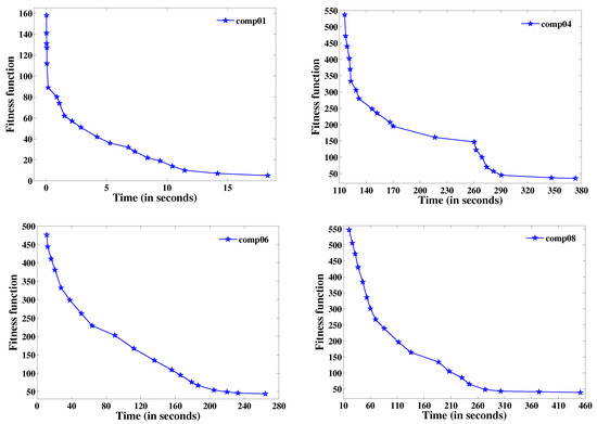
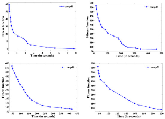
Figure 8. Best fitness function value versus time for CB-CTP instances.

The fitness function values obtained for all 21 instances from all 20 independent trials are summarized by the boxplot in Figure 9.

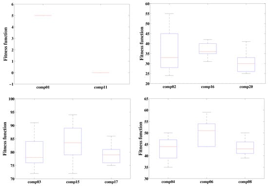
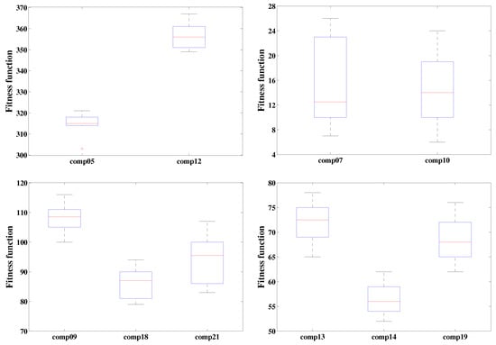
Figure 9. Boxplots of results obtained for CB-CTP instances.

5.2.1. Comparative Experiments

In this segment, we compare the performance of GAILS with the performance of the five finalist algorithms in the third track of ITC2007. These algorithms C1, C2, C3, C4, and C5 were proposed by [29,32,35,39,65], respectively. For all the 21 CB-CTP instances, each of these five algorithms was run independently for ten trials. A ranking was then calculated based on these 50 outcomes for each problem instance. Finally, a ranking was established according to the ranks realized on these 21 CB-CTP instances. Rank-wise, these five finalists were C1, C2, C3, C4, and C5. The detailed results of their outcomes in terms of $f_{\min },f_{\max },f_{\mathrm{avg}},\mathrm{and}\varsigma$ are given in Table 16.

Table 16. Comparison of different algorithms on CB-CTP instances.

Instance	C1				C2				C3				C4				C5
	${\mathit{f}}_{\mathbf{min}}$	${\mathit{f}}_{\mathbf{max}}$	${\mathit{f}}_{\mathbf{avg}}$	$\mathbf{\varsigma }$	${\mathit{f}}_{\mathbf{min}}$	${\mathit{f}}_{\mathbf{max}}$	${\mathit{f}}_{\mathbf{avg}}$	$\mathbf{\varsigma }$	${\mathit{f}}_{\mathbf{min}}$	${\mathit{f}}_{\mathbf{max}}$	${\mathit{f}}_{\mathbf{avg}}$	$\mathbf{\varsigma }$	${\mathit{f}}_{\mathbf{min}}$	${\mathit{f}}_{\mathbf{max}}$	${\mathit{f}}_{\mathbf{avg}}$	$\mathbf{\varsigma }$	${\mathit{f}}_{\mathbf{min}}$	${\mathit{f}}_{\mathbf{max}}$	${\mathit{f}}_{\mathbf{avg}}$	$\mathbf{\varsigma }$
comp01	5	5	5	0	5	5	5	0	5	6	$5.1$	$0.316$	5	9	$6.7$	$1.059$	10	68	27	$19.66$
comp02	51	70	$61.3$	$6.783$	55	74	$61.2$	$5.329$	50	76	$65.6$	$7.905$	111	168	$142.7$	$21.25$	111	146	$131.1$	$11.05$
comp03	84	103	$94.8$	$5.922$	71	101	$84.5$	$8.086$	82	95	$89.1$	$4.932$	128	188	$160.3$	$18.18$	119	167	$138.4$	$14.64$
comp04	37	48	$42.8$	$3.490$	43	53	$46.9$	$3.315$	35	44	$39.2$	$2.530$	72	91	82	$6.992$	72	110	$90.2$	$10.97$
comp05	330	379	$343.5$	$14.62$	309	346	326	$14.23$	312	353	$334.5$	$13.54$	410	691	$525.4$	$89.45$	426	2000	$811.5$	$628.80$
comp06	48	65	$56.8$	$5.350$	53	80	$69.4$	$8.656$	69	84	$74.1$	$4.408$	100	129	$110.8$	$8.377$	130	181	$149.3$	$17.20$
comp07	20	45	$33.9$	$7.172$	28	49	$41.5$	$6.671$	42	56	$49.8$	$4.467$	57	89	$76.6$	$10.15$	110	191	$153.4$	$22.53$
comp08	41	55	$46.5$	$4.353$	49	58	$52.6$	$2.989$	40	50	46	$2.828$	77	90	$81.7$	$4.448$	83	116	$96.5$	$9.733$
comp09	109	117	$113.1$	$2.767$	105	127	$116.5$	$6.900$	110	121	$113.3$	$3.234$	150	178	$164.1$	$9.769$	139	157	$148.9$	$6.967$
comp10	16	27	$21.3$	$4.423$	21	48	$34.8$	$9.343$	27	49	$36.9$	$6.454$	71	96	$81.3$	$7.818$	85	122	$101.3$	$12.693$
comp11	0	0	0	0	0	0	0	0	0	0	0	0	0	2	$0.3$	$0.675$	3	8	$5.7$	$1.337$
comp12	333	367	$351.6$	$10.352$	343	380	$360.1$	$12.441$	351	378	$361.6$	$8.527$	442	544	$485.1$	$32.78$	408	487	$445.3$	$29.42$
comp13	66	81	$73.9$	$4.533$	73	87	$79.2$	$4.541$	68	82	$76.1$	$4.202$	98	125	$110.4$	$9.204$	113	145	$122.9$	$10.556$
comp14	59	69	$61.8$	$2.936$	57	77	$65.9$	$6.226$	59	68	$62.3$	$3.433$	90	108	99	$5.077$	84	127	$105.9$	$12.71$
comp15	84	103	$94.8$	$5.922$	71	101	$84.5$	$8.086$	82	95	$89.1$	$4.932$	128	188	$160.3$	$18.18$	119	167	138	$14.79$
comp16	34	49	$41.2$	$4.826$	39	57	$49.1$	$5.567$	40	60	$50.2$	$6.477$	81	103	$92.6$	$6.620$	84	127	$107.3$	$11.98$
comp17	83	92	$86.6$	$2.547$	91	111	$100.7$	$6.848$	102	115	$107.3$	$4.423$	124	161	$143.4$	$13.56$	152	178	$166.6$	$9.454$
comp18	83	102	$91.7$	$5.539$	69	93	$80.7$	$6.255$	68	80	$73.3$	$3.773$	116	145	$129.4$	$9.312$	110	142	$126.8$	$11.033$
comp19	62	74	$68.8$	$3.676$	65	77	$69.5$	$4.353$	75	85	$79.6$	$3.373$	107	184	$132.8$	$23.612$	111	148	$125.4$	$12.633$
comp20	27	44	$34.3$	$4.855$	47	72	$60.9$	$8.171$	61	71	65	$3.590$	88	109	$97.5$	$6.399$	144	201	$179.3$	$17.06$
comp21	103	121	108	$6.683$	106	137	$124.7$	$8.693$	123	150	$138.1$	$8.80$	174	210	$185.3$	$12.81$	169	202	$185.8$	$12.02$

In order to compare different algorithms statistically, their t-test comparison was performed, and the obtained results are presented in Table 17. This statistical comparison was implemented by using $n_1+n_2-2$ degree of freedom at $0.05$ level of significance, where $n_1$ and $n_2$ are the sample sizes of the first and second samples, respectively. The t-test comparison of the two algorithms is also demonstrated as “$s+$”, “$s-$”, “+”, “−”, or “∼”. The table clearly shows that GAILS outperforms the other algorithms in the majority of the problem instances.

Table 17. The t-test comparison of different algorithms on CB-CTP instances.

Instance	GAILS vs. C1	GAILS vs. C2	GAILS vs. C3	GAILS vs. C4	GAILS vs. C5
comp01	∼	∼	+	$s+$	$s+$
comp02	$s+$	$s+$	$s+$	$s+$	$s+$
comp03	$s+$	+	$s+$	$s+$	$s+$
comp04	∼	$s+$	$s-$	$s+$	$s+$
comp05	$s+$	$s+$	$s+$	$s+$	$s+$
comp06	$s+$	$s+$	$s+$	$s+$	$s+$
comp07	$s+$	$s+$	$s+$	$s+$	$s+$
comp08	+	$s+$	+	$s+$	$s+$
comp09	$s+$	$s+$	$s+$	$s+$	$s+$
comp10	$s+$	$s+$	$s+$	$s+$	$s+$
comp11	∼	∼	∼	+	$s+$
comp12	∼	+	+	$s+$	$s+$
comp13	+	$s+$	$s+$	$s+$	$s+$
comp14	$s+$	$s+$	$s+$	$s+$	$s+$
comp15	$s+$	+	$s+$	$s+$	$s+$
comp16	$s+$	$s+$	$s+$	$s+$	$s+$
comp17	$s+$	$s+$	$s+$	$s+$	$s+$
comp18	$s+$	$s-$	$s-$	$s+$	$s+$
comp19	+	+	$s+$	$s+$	$s+$
comp20	+	$s+$	$s+$	$s+$	$s+$
comp21	$s+$	$s+$	$s+$	$s+$	$s+$

It is simple to arrive at the conclusion that an algorithm that relies solely on exploration or exploitation cannot be the best option for solving CB-CTP. Therefore, a suitable choice that can significantly enhance the solution quality of CB-CTP is the hybridization of an exploration-based algorithm (GA) with an appropriate exploitation-based algorithm (ILS).

5.2.2. Comparison with Existing Algorithms

GAILS is now being compared to the 20 existing state-of-the-art algorithms tested on CB-CTP instances. These algorithms are listed in Table 18. The comparison of these algorithms with GAILS is demonstrated in Table 19. Entries in this table signify a feasible solution’s measured best fitness function value. Here, the entry “−” denotes an untried instance in the experiment.

Table 18. Keys of the algorithms used for comparison.

No.	Key	Algorithm	Reference
1	GAILS	GA with ILS	Proposed method
2	D1	Electromagnetic-like mechanism and great deluge algorithm	[22]
3	D2	Constraint-based solver	[35]
4	D3	Hybrid adaptive TS algorithm	[32]
5	D4	TS algorithm with relaxed stopping condition	[32]
6	D5	Combination of great deluge and TS algorithms	[23]
7	D6	Dynamic TS algorithm	[66]
8	D7	Integer programming approach	[67]
9	D8	General purpose constraint satisfaction problem solver	[29]
10	D9	Memetic TS algorithm using random neighborhood	[68]
11	D10	Memetic TS algorithm using general neighborhood	[68]
12	D11	Repair based LS algorithm	[39]
13	D12	Heuristic local search based on the principles of threshold accepting	[65]
14	D13	Hybrid LS algorithm	[69]
15	D14	ABC algorithm	[41]
16	D15	New swarm intelligence algorithm based on the ABC algorithm	[42]
17	D16	Harmony search algorithm	[38]
18	D17	Two mixed-integer programming techniques with flow formulation	[70]
19	D18	Adaptive large neighborhood search	[71]
20	D19	Localized island model GA with dual dynamic migration policy	[72]
21	D20	A competition-guided multi-neighborhood local search algorithm	[45]

Table 19. Comparison results on CB-CTP instances.

Instance	GAILS	D1	D2	D3	D4	D5	D6	D7	D8	D9	D10	D11	D12	D13	D14	D15	D16	D17	D18	D19	D20
comp01	5	5	5	5	5	5	5	13	5	5	5	9	5	5	23	5	322	5	5	5	5
comp02	24	39	43	34	56	39	75	43	50	30	27	103	108	41	190	86	732	8	33	382	39
comp03	72	76	72	70	79	73	93	76	82	70	73	101	115	66	171	101	665	38	71	82	70
comp04	35	35	35	38	38	36	45	38	35	35	39	55	67	35	132	57	577	35	35	38	36
comp05	303	315	298	298	316	309	326	314	312	300	312	370	408	301	1483	377	1297	186	292	5	303
comp06	44	50	41	47	55	43	62	41	69	42	30	112	94	43	237	87	879	16	39	0	42
comp07	7	12	14	19	26	17	38	19	42	8	10	97	56	18	259	61	930	6	12	0	13
comp08	39	37	39	43	42	40	50	43	40	37	37	72	75	39	154	60	645	37	39	0	39
comp09	100	104	103	99	104	104	119	102	110	100	100	132	153	96	190	127	685	74	100	0	100
comp10	6	10	9	16	19	12	27	14	27	7	5	74	66	15	210	51	816	4	11	0	13
comp11	0	0	0	0	0	0	0	0	0	0	0	1	0	0	18	0	179	0	0	0	0
comp12	349	337	331	320	342	334	358	405	351	323	330	393	430	320	583	397	1398	142	310	242	332
comp13	65	61	66	65	72	67	77	68	68	59	62	97	101	64	156	90	694	59	60	0	65
comp14	52	53	53	52	57	54	59	54	59	55	53	87	88	53	165	77	702	44	52	0	53
comp15	72	73	84	69	79	88	87	−	82	70	73	119	128	66	193	92	665	38	67	0	71
comp16	31	32	34	38	46	52	47	−	40	18	18	84	81	28	215	83	827	13	29	32	31
comp17	75	72	83	80	88	88	86	−	102	65	61	152	124	71	206	110	830	44	63	81	69
comp18	79	77	83	67	75	84	71	−	68	72	79	110	116	69	122	97	510	36	65	0	74
comp19	62	60	62	59	64	71	74	−	75	58	57	111	107	60	205	82	608	56	61	75	62
comp20	25	22	27	35	32	34	54	−	61	11	4	144	88	29	263	77	950	0	21	46	28
comp21	83	95	103	105	107	98	117	−	123	86	90	169	174	89	233	74	835	57	92	0	94

Table 19 demonstrates that GAILS can deliver competitive results with current state-of-the-art algorithms. From the obtained results, it can be observed that the appropriate combination of a population-based algorithm emphasizing exploration and a local area-based algorithm emphasizing exploitation can help to reduce the values of the fitness function and produce good results for the CB-CTP in comparison to other existing algorithms.

6. Conclusions

An exploration-and-exploitation-based hybrid approach is proposed by combining GA with ILS to solve the PE-CTP and CB-CTP. This hybrid approach is influential yet straightforward and manages to produce several improved results. The algorithm uses ILS, which utilizes various kinds of moves for neighborhood and perturbation. Furthermore, it enables the refinement of the entire population generated by GA. The algorithm is tested over 11 benchmark PE-CTP instances and 21 benchmark CB-CTP instances in two separate experiments. In the first experiment, all the PE-CTP instances are run, each with different execution times, and the least fitness function value is used as their performance measure. A comparison with existing approaches has been carried out to demonstrate its effectiveness over other approaches. Statistically, t-test comparisons also displayed the dominance of GAILS. In this experiment, it is also observed that the solution quality improves a lot for the extended time limit, establishing that by using the perturbation operator, GAILS is capable of avoiding the local optimal. In the second experiment, the performance of GAILS is measured by running each problem instance for twenty trials, and each trial lasts for 600 s. Its performance is also compared with several other existing algorithms. The computational results show that the proposed algorithm can produce competitive results when compared with existing state-of-the-art algorithms.

Among the timetabling (scheduling) problems, the UCTP is one of the most complex problems, with many decision variables and various soft and hard constraints. Problems with formally simpler problem statements such as the industrial capacity planning [73,74] are sometimes large-scale, and the standard approach of reducing the problem to an integer linear programming problem leads to a huge increase in the number of variables, so in practice, it is necessary to apply various combinations of heuristic algorithms, including evolutionary algorithms, greedy search algorithms, and local search.

Our proposed algorithm gives encouraging results on several instances of rather complex problems of two types. Therefore, further research can be aimed at applying this approach to other scheduling problems; for example, to the problem of capacity utilization planning. The limits of applicability of the proposed approach can be explored and, possibly, extended to other complex optimization problems with Boolean variables for which local search methods are known to be effective.

References

- Wren, A. Scheduling, timetabling and rostering—A special relationship? In Practice and theory of automated timetabling; Springer: Cham, Switzerland, 1996; pp. 46–75. [Google Scholar]
- Di Gaspero, L.; McCollum, B.; Schaerf, A. The Second International Timetabling Competition (ITC-2007): Curriculum-Based Course Timetabling (Track 3); Technical Report, QUB/IEEE/Tech/ITC2007/CurriculumCTT/v1.0; Queen’s University: Belfast, UK, 2007. [Google Scholar]
- Gotlieb, C. The construction of class-teacher timetables. In Proceedings of the International Federation of Information Processing Congress, Munich, Germany, 27 August–1 September 1962; Volume 62, pp. 73–77. [Google Scholar]
- Carter, M.W.; Laporte, G. Recent developments in practical course timetabling. In Practice and Theory of Automated Timetabling II; Springer: Cham, Switzerland, 1998; pp. 3–19. [Google Scholar]
- Chiarandini, M.; Birattari, M.; Socha, K.; Rossi-Doria, O. An effective hybrid algorithm for university course timetabling. J. Sched. 2006, 9, 403–432. [Google Scholar] [CrossRef]
- Jat, S.N.; Yang, S. A hybrid genetic algorithm and tabu search approach for post enrolment course timetabling. J. Sched. 2011, 14, 617–637. [Google Scholar] [CrossRef]
- Socha, K.; Knowles, J.; Sampels, M. A max-min ant system for the university course timetabling problem. In Ant Algorithms; Springer: Cham, Switzerland, 2002; pp. 1–13. [Google Scholar]
- Rossi-Doria, O.; Sampels, M.; Birattari, M.; Chiarandini, M.; Dorigo, M.; Gambardella, L.M.; Knowles, J.; Manfrin, M.; Mastrolilli, M.; Paechter, B.; et al. A comparison of the performance of different metaheuristics on the timetabling problem. In Practice and Theory of Automated Timetabling IV; Springer: Cham, Switzerland, 2003; pp. 329–351. [Google Scholar]
- Burke, E.K.; Kendall, G.; Soubeiga, E. A tabu-search hyperheuristic for timetabling and rostering. J. Heuristics 2003, 9, 451–470. [Google Scholar] [CrossRef]
- Burke, E.K.; McCollum, B.; Meisels, A.; Petrovic, S.; Qu, R. A graph-based hyper-heuristic for educational timetabling problems. Eur. J. Oper. Res. 2007, 176, 177–192. [Google Scholar] [CrossRef]
- Abuhamdah, A.; Ayob, M. Adaptive randomized descent algorithm for solving course timetabling problems. Int. J. Phys. Sci. 2010, 5, 2516–2522. [Google Scholar]
- Al-Betar, M.A.; Khader, A.T. A harmony search algorithm for university course timetabling. Ann. Oper. Res. 2012, 194, 3–31. [Google Scholar] [CrossRef]
- Cambazard, H.; Hebrard, E.; O’Sullivan, B.; Papadopoulos, A. Local search and constraint programming for the post enrolment-based course timetabling problem. Ann. Oper. Res. 2012, 194, 111–135. [Google Scholar] [CrossRef]
- Abuhamdah, A.; Ayob, M.; Kendall, G.; Sabar, N.R. Population based Local Search for university course timetabling problems. Appl. Intell. 2014, 40, 44–53. [Google Scholar] [CrossRef]
- Méndez-Díaz, I.; Zabala, P.; Miranda-Bront, J.J. An ILP based heuristic for a generalization of the post-enrollment course timetabling problem. Comput. Oper. Res. 2016, 76, 195–207. [Google Scholar] [CrossRef]
- Goh, S.L.; Kendall, G.; Sabar, N.R. Simulated annealing with improved reheating and learning for the post enrolment course timetabling problem. J. Oper. Res. Soc. 2019, 70, 873–888. [Google Scholar] [CrossRef]
- Blum, C.; Roli, A. Metaheuristics in combinatorial optimization: Overview and conceptual comparison. Acm Comput. Surv. (CSUR) 2003, 35, 268–308. [Google Scholar] [CrossRef]
- Abdullah, S.; Turabieh, H. Generating university course timetable using genetic algorithms and local search. In Proceedings of the Third International Conference on Convergence and Hybrid Information Technology (ICCIT’08), Busan, Republic of Korea, 11–13 November 2008; Volume 1, pp. 254–260. [Google Scholar]
- Abdullah, S.; Burke, E.K.; McCollum, B. A hybrid evolutionary approach to the university course timetabling problem. In Proceedings of the 2007 IEEE Congress on Evolutionary Computation, Singapore, 25–28 September 2007; pp. 1764–1768. [Google Scholar]
- Jat, S.N.; Yang, S. A guided search genetic algorithm for the university course timetabling problem. In Proceedings of the Multidisciplinary International Conference on Scheduling: Theory and Applications IV, Dublin, Ireland, 10–12 August 2009; pp. 180–191. [Google Scholar]
- Yang, S.; Jat, S.N. Genetic algorithms with guided and local search strategies for university course timetabling. IEEE Trans. Syst. Man Cybern. Part Appl. Rev. 2011, 41, 93–106. [Google Scholar] [CrossRef]
- Abdullah, S.; Turabieh, H.; McCollum, B.; McMullan, P. A hybrid metaheuristic approach to the university course timetabling problem. J. Heuristics 2012, 18, 1–23. [Google Scholar] [CrossRef]
- Shaker, K.; Abdullah, S.; Alqudsi, A.; Jalab, H. Hybridizing Meta-heuristics Approaches for Solving University Course Timetabling Problems. In Rough Sets and Knowledge Technology; Springer: Cham, Switzerland, 2013; pp. 374–384. [Google Scholar]
- Badoni, R.P.; Gupta, D.; Mishra, P. A new hybrid algorithm for university course timetabling problem using events based on groupings of students. Comput. Ind. Eng. 2014, 78, 12–25. [Google Scholar] [CrossRef]
- Fong, C.W.; Asmuni, H.; McCollum, B. A hybrid swarm-based approach to university timetabling. IEEE Trans. Evol. Comput. 2015, 19, 870–884. [Google Scholar] [CrossRef]
- Unprasertporn, T.; Lohpetch, D. An Outperforming Hybrid Discrete Particle Swarm Optimization for Solving the Timetabling Problem. In Proceedings of the 12th International Conference on Knowledge and Smart Technology (KST’20), Pattaya, Thailand, 29 January–1 February 2020; pp. 18–23. [Google Scholar]
- Rezaeipanah, A.; Matoori, S.S.; Ahmadi, G. A hybrid algorithm for the university course timetabling problem using the improved parallel genetic algorithm and local search. Appl. Intell. 2021, 51, 467–492. [Google Scholar] [CrossRef]
- Chen, M.C.; Goh, S.L.; Sabar, N.R.; Kendall, G. A survey of university course timetabling problem: Perspectives, trends and opportunities. IEEE Access 2021, 9, 106515–106529. [Google Scholar] [CrossRef]
- Atsuta, M.; Nonobe, K.; Ibaraki, T. ITC2007 Track2: An Approach Using General CSP solver. In Proceedings of the Practice and Theory of Automated Timetabling (PATAT 2008), Montreal, QC, Canada, 19–22 August 2008. [Google Scholar]
- Bellio, R.; Ceschia, S.; Di Gaspero, L.; Schaerf, A.; Urli, T. Feature-based tuning of simulated annealing applied to the curriculum-based course timetabling problem. Comput. Oper. Res. 2016, 65, 83–92. [Google Scholar] [CrossRef]
- Lach, G.; Lübbecke, M.E. Curriculum based course timetabling: New solutions to Udine benchmark instances. Ann. Oper. Res. 2012, 194, 255–272. [Google Scholar] [CrossRef]
- Lü, Z.; Hao, J.K. Adaptive tabu search for course timetabling. Eur. J. Oper. Res. 2010, 200, 235–244. [Google Scholar] [CrossRef]
- Pillay, N.; Özcan, E. Automated generation of constructive ordering heuristics for educational timetabling. Ann. Oper. Res. 2019, 275, 181–208. [Google Scholar] [CrossRef]
- Badoni, R.P.; Gupta, D.; Lenka, A.K. A new approach for university timetabling problems. Int. J. Math. Oper. Res. 2014, 6, 236–257. [Google Scholar] [CrossRef]
- Müller, T. ITC2007 solver description: A hybrid approach. Ann. Oper. Res. 2009, 172, 429–446. [Google Scholar] [CrossRef][Green Version]
- Azlan, A.; Hussin, N.M. Implementing graph coloring heuristic in construction phase of curriculum-based course timetabling problem. In Proceedings of the 2013 IEEE Symposium on Computers & Informatics (ISCI), Langkawi, Malaysia, 7–9 April 2013; pp. 25–29. [Google Scholar]
- Rangel-Valdez, N.; Torres-Jimenez, J.; Jasso-Luna, J.O.; Rodriguez-Chavez, M.H. SAT Model for the Curriculum-Based Course Timetabling Problem. Adv. Soft Comput. Tech. 2013, 68, 45–55. [Google Scholar] [CrossRef]
- Wahid, J.; Hussin, N.M. Harmony Search Algorithm for Curriculum-Based Course Timetabling Problem. Int. J. Soft Comput. Softw. Eng. 2013, 3, 365–371. [Google Scholar]
- Clark, M.; Henz, M.; Love, B. Quikfix a Repair-Based Timetable Solver. In Proceedings of the 7th International Conference on the Practice and Theory of Automated Timetabling, PATAT, Montréal, QC, Canada, 18–22 August 2008; Available online: http://www.comp.nus.edu.sg/~henz/publications/ps/PATAT2008.pdf (accessed on 1 July 2023).
- Petrovic, S.; Burke, E.K. University timetabling. In Handbook of Scheduling: Algorithms, Models, and Performance Analysis; Leung, J., Ed.; CRC Press: Boca Raton, FL, USA, 2004; Chapter 45; pp. 1–23. [Google Scholar]
- Junaedi, D.; Maulidevi, N.U. Solving Curriculum-Based Course Timetabling Problem with Artificial Bee Colony Algorithm. In Proceedings of the First International Conference on Informatics and Computational Intelligence (ICI), Bandung, Indonesia, 12–14 December 2011; pp. 112–117. [Google Scholar]
- Agahian, S.; Pehlivan, H.; Dehkharghani, R. Adaptation and Use of Artificial Bee Colony Algorithm to Solve Curriculum-based Course Time-Tabling Problem. In Proceedings of the Fifth International Conference on Intelligent Systems, Modelling and Simulation (ISMS), Langkawi, Malaysia, 27–29 January 2014; pp. 77–82. [Google Scholar]
- Akkan, C.; Gülcü, A. A bi-criteria hybrid Genetic Algorithm with robustness objective for the course timetabling problem. Comput. Oper. Res. 2018, 90, 22–32. [Google Scholar] [CrossRef]
- Banbara, M.; Inoue, K.; Kaufmann, B.; Okimoto, T.; Schaub, T.; Soh, T.; Tamura, N.; Wanko, P. teaspoon: Solving the curriculum-based course timetabling problems with answer set programming. Ann. Oper. Res. 2019, 275, 3–37. [Google Scholar] [CrossRef]
- Song, T.; Chen, M.; Xu, Y.; Wang, D.; Song, X.; Tang, X. Competition-guided multi-neighborhood local search algorithm for the university course timetabling problem. Appl. Soft Comput. 2021, 110, 107624. [Google Scholar] [CrossRef]
- Abdipoor, S.; Yaakob, R.; Goh, S.L.; Abdullah, S. Meta-heuristic approaches for the University Course Timetabling Problem. Intell. Syst. Appl. 2023, 19, 200253. [Google Scholar] [CrossRef]
- Papadimitriou, C.H.; Steiglitz, K. Combinatorial Optimization: Algorithms and Complexity; Courier Dover Publications: Mineola, NY, USA, 1998. [Google Scholar]
- Golberg, D.E. Genetic Algorithms in Search, Optimization, and Machine Learning; Addion Wesley: Boston, MA, USA, 1989; Volume 1989. [Google Scholar]
- Hageman, J.; Wehrens, R.; Van Sprang, H.; Buydens, L. Hybrid genetic algorithm–Tabu search approach for optimising multilayer optical coatings. Anal. Chim. Acta 2003, 490, 211–222. [Google Scholar] [CrossRef]
- Fatourechi, M.; Bashashati, A.; Ward, R.K.; Birch, G.E. A hybrid genetic algorithm approach for improving the performance of the LF-ASD brain computer interface. In Proceedings of the IEEE International Conference on Acoustics, Speech, and Signal Processing, Philadelphia, PA, USA, 23 March 2005; Volume 5, pp. 345–348. [Google Scholar]
- Sastry, K.; Goldberg, D.; Kendall, G. Genetic algorithms. In Search Methodologies; Springer: Cham, Switzerland, 2005; pp. 97–125. [Google Scholar]
- Datta, D.; Deb, K.; Fonseca, C.M. Multi-objective evolutionary algorithm for university class timetabling problem. In Evolutionary Scheduling; Springer: Cham, Switzerland, 2007; pp. 197–236. [Google Scholar]
- Lourenço, H.R.; Martin, O.C.; Stützle, T. Iterated Local Search. Sci. Kluwer 2002, 57, 321–353. [Google Scholar]
- Turabieh, H.; Abdullah, S. Incorporating tabu search into memetic approach for enrolment-based course timetabling problems. In Proceedings of the Second Conference on Data Mining and Optimization (DMO’09), Kajand, Malaysia, 27–28 October 2009; pp. 115–119. [Google Scholar]
- Abdullah, S.; Burke, E.K.; McCollum, B. Using a randomised iterative improvement algorithm with composite neighbourhood structures for the university course timetabling problem. In Metaheuristics; Springer: Cham, Switzerland, 2007; pp. 153–169. [Google Scholar]
- Mcmullan, P. An extended implementation of the great deluge algorithm for course timetabling. In Proceedings of the International Conference on Computational Science (ICCS’07), Beijing, China, 27–30 May 2007; Springer: Cham, Switzerland, 2007; pp. 538–545. [Google Scholar]
- Landa-Silva, D.; Obit, J.H. Great deluge with non-linear decay rate for solving course timetabling problems. In Proceedings of the Fourth International Conference on Intelligent Systems (IS’08), Varna, Bulgaria, 6–8 September 2008; Volume 1, pp. 8–11. [Google Scholar]
- Obit, J.; Landa-Silva, D.; Ouelhadj, D.; Sevaux, M. Non-linear great deluge with learning mechanism for solving the course timetabling problem. In Proceedings of the Eighth Metaheuristics International Conference (MIC’09), Hamburg, Germany, 13–16 July 2009. [Google Scholar]
- Turabieh, H.; Abdullah, S.; McCollum, B.; McMullan, P. Fish swarm intelligent algorithm for the course timetabling problem. In Rough Set and Knowledge Technology; Springer: Cham, Switzerland, 2010; pp. 588–595. [Google Scholar]
- Abuhamdah, A.; Ayob, M. MPCA-ARDA for solving course timetabling problems. In Proceedings of the Third Conference on Data Mining and Optimization (DMO’11), Putrajaya, Malaysia, 28–29 June 2011; pp. 171–177. [Google Scholar]
- Bolaji, A.L.; Khader, A.T.; Al-Betar, M.A.; Awadallah, M.A. University course timetabling using hybridized artificial bee colony with hill climbing optimizer. J. Comput. Sci. 2014, 5, 809–818. [Google Scholar] [CrossRef]
- Fong, C.W.; Asmuni, H.; McCollum, B.; McMullan, P.; Omatu, S. A new hybrid imperialist swarm-based optimization algorithm for university timetabling problems. Inf. Sci. 2014, 283, 1–21. [Google Scholar] [CrossRef]
- Al-Betar, M.A.; Khader, A.T.; Zaman, M. University course timetabling using a hybrid harmony search metaheuristic algorithm. IEEE Trans. Syst. Man Cybern. Part Appl. Rev. 2012, 42, 664–681. [Google Scholar] [CrossRef]
- Lohpetch, D.; Jaengchuea, S. A hybrid multi-objective genetic algorithm with a new local search approach for solving the post enrolment based course timetabling problem. In Recent Advances in Information and Communication Technology 2016; Springer: Cham, Switzerland, 2016; pp. 195–206. [Google Scholar]
- Geiger, M.J. Applying the threshold accepting metaheuristic to curriculum based course timetabling. Ann. Oper. Res. 2012, 194, 189–202. [Google Scholar] [CrossRef][Green Version]
- De Cesco, F.; Di Gaspero, L.; Schaerf, A. Benchmarking Curriculum-Based Course Timetabling: Formulations, Data Formats, Instances, Validation, and Results. In Proceedings of the 7th international Conference on the Practice and Theory of Automated Timetabling, PATAT, Montréal, QC, Canada, 18–22 August 2008. [Google Scholar]
- Lach, G.; Lübbecke, M. Curriculum based course timetabling: Optimal solutions to the udine benchmark instances. In Proceedings of the Seventh International Conference on the Practice and Theory of Automated Timetabling, Montréal, QC, Canada, 18–22 August 2008. [Google Scholar]
- Abdullah, S.; Turabieh, H. On the use of multi neighbourhood structures within a Tabu-based memetic approach to university timetabling problems. Inf. Sci. 2012, 191, 146–168. [Google Scholar] [CrossRef]
- Bellio, R.; Di Gaspero, L.; Schaerf, A. Design and statistical analysis of a hybrid local search algorithm for course timetabling. J. Sched. 2012, 15, 49–61. [Google Scholar] [CrossRef]
- Bagger, N.C.F.; Kristiansen, S.; Sørensen, M.; Stidsen, T.R. Flow formulations for curriculum-based course timetabling. Ann. Oper. Res. 2019, 280, 121–150. [Google Scholar] [CrossRef]
- Kiefer, A.; Hartl, R.F.; Schnell, A. Adaptive large neighborhood search for the curriculum-based course timetabling problem. Ann. Oper. Res. 2017, 252, 255–282. [Google Scholar] [CrossRef]
- Gozali, A.A.; Kurniawan, B.; Weng, W.; Fujimura, S. Solving university course timetabling problem using localized island model genetic algorithm with dual dynamic migration policy. IEEJ Trans. Electr. Electron. Eng. 2020, 15, 389–400. [Google Scholar] [CrossRef]
- Kazakovtsev, L.A.; Gudyma, M.N.; Antamoshkin, A.N. Genetic Algorithm with Greedy Heuristic for Capacity Planning. In Proceedings of the International Congress on Ultra Modern Telecommunications and Control Systems and Workshops, St. Petersburg, Russia, 6–8 October 2014; pp. 607–613. [Google Scholar]
- Kazakovtsev, L.; Kovlovskaya, E.; Rozhnov, I.; Patsuk, O. A genetic algorithm with greedy crossover and elitism for capacity planning. Facta Univ. Ser. Math. Inform. 2023, 37, 993–1006. [Google Scholar]
Disclaimer/Publisher’s Note: The statements, opinions and data contained in all publications are solely those of the individual author(s) and contributor(s) and not of MDPI and/or the editor(s). MDPI and/or the editor(s) disclaim responsibility for any injury to people or property resulting from any ideas, methods, instructions or products referred to in the content. |
© 2023 by the authors. Licensee MDPI, Basel, Switzerland. This article is an open access article distributed under the terms and conditions of the Creative Commons Attribution (CC BY) license (https://creativecommons.org/licenses/by/4.0/).