A Novel Non-Ferrous Metals Price Forecast Model Based on LSTM and Multivariate Mode Decomposition

Abstract

Non-ferrous metals are important bulk commodities and play a significant part in the development of society. Their price forecast is of great reference value for investors and policymakers. However, developing a robust price forecast model is tricky due to the price’s drastic fluctuations. In this work, a novel fusion model based on Complete Ensemble Empirical Mode Decomposition with Adaptive Noise (CEEMDAN), Singular Spectrum Analysis (SSA), and Long Short-Term Memory (LSTM) is constructed for non-ferrous metals price forecast. Considering the complexity of their price change, the dual-stage signal preprocessing which combines CEEMDAN and SSA is utilized. Firstly, we use the CEEMDAN algorithm to decompose the original nonlinear price sequence into multiple Intrinsic Mode Functions (IMFs) and a residual. Secondly, the component with maximum sample entropy is decomposed by SSA; this is the so-called Multivariate Mode Decomposition (MMD). A series of experimental results show that the proposed MMD-LSTM method is more stable and robust than the other seven benchmark models, providing a more reasonable scheme for the price forecast of non-ferrous metals.

1. Introduction

This paper firstly introduces the background of the non-ferrous metals price forecast to show that it is of great significance to accurately predict the price changes, which should be extensively carried out in academic research. Nextly, the related literature is reviewed to provide an overview of existing prediction methods and highlight the novelty of this work.

1.1. Background

Non-ferrous metals are important commodities and play a vital role in economic activity. In most countries, metal minerals are the lifeblood of their economy. Moreover, metal aluminum, copper and zinc, are indispensable raw materials for industry. Therefore, for machinery manufacturing enterprises, price fluctuations will affect their procurement plans. In addition, metals have both commercial and financial attributes. Take gold as an example, it is a special non-ferrous metal known as an asset tool used to balance volatility in a particular portfolio. Also, the fluctuation of its price is a barometer of economic changes, which helps financial participants avoid the risk of mineral market through the metals arbitrage trade [1,2,3]. Consequently, the importance of accurately predicting non-ferrous metals price is self-explanatory. According to the professional study, these nonferrous metals price are influenced by various realistic factors, such as production costs, supply and demand relation, as well as the dollar exchange rate. Even more, these different factors are coupled and related to each other, which brings difficulty in accurately predicting prices.

Various model methods have been proposed for nearly a decade to predict non-ferrous metals prices. In the literature, these prediction models can be Classified into single models and those fusion models. Prediction based on singles model mainly includes statistical approaches and artificial intelligence (AI) technology. Nevertheless, financial time series have a complex nonlinear structure, and single model-based prediction cannot adequately capture the subtle underlying relationships. The fusion model is constructed by making the best of the merit of each model to improve prediction accuracy. Here, the types of fusion models are presented as follows: (1) prediction model optimized using intelligence algorithm; (2) combination of different prediction models; (3) combining signal decomposition algorithm and prediction model.

1.2. Related Literature

1.2.1. Single Model Based Prediction

In the past, single model-based prediction methods have been mostly used during metals price prediction. Dooly and Lenihan utilized autoregressive integrated moving average (ARIMA) to forecast the monthly collapse prices of lead and zinc [4]. As a result, ARIMA modeling provided slightly better predictions than lagging forward price modeling. Meanwhile, a vast amount of AI models were gradually used to predict data series, such as Support Vector Machine, Decision Tree, Extreme Learning Machine and so on [5,6,7]. Liu Chang et al utilized the decision tree approach to predict future copper prices in 2017 [8]. This method reliably predicted copper prices in the short and long term, with an average absolute percentage error of below 4%. In recent, the Deep Belief Network was used by Zhang et al to predict gold prices [9]. In general, improved DBN had higher accuracy compared to traditional neural networks and linear models. Although the Artificial Neural Network (ANN) models outperform the conventional statistical models, they cannot still accurately capture the underlying feature information due to complex nonlinear structure of financial series.

1.2.2. Fusion Model Based Prediction

The fusion model based prediction method combines several excellent algorithms to improve the robustness of forecast model, which breaks the limitation of single model [10,11]. For the first type of fusion model, it is performed using optimization algorithm to optimize the parameters of prediction model. For instance, Hesam Dehghani et al. applied Bat Algorithm to improve the classical time series function, and the final determined equation can better predict the copper price [12]. Shao Bilin et al. proposed a nickel metal price prediction model based on improved Particle Swarm Optimization algorithm and LSTM neural network to effectively improve forecast performance [13].

For the second type of fusion model, the forecast precision is improved by combining two or more forecast models. Siti Roslindar Yaziz et al. proposed ARIMA and Symmetric GARCH-type Models for Malaysian gold price prediction and significantly improved the prediction accuracy [14]. Although these equation models can reflect internal regularity, they are only suitable for short-term predictions because these equations are established based on the assumption of independence of local laws. In 2017, Hou Muzhou and Yang Yunlei et al proposed the hybrid constructive neural network method (HCNNM) based on Radial Basis Function (RBF) to fix the impact values in the raw data as a functional jump-point manner and to more accurately predict future tungsten prices [15]. In recent years, Andres Vidal and Werner Kristjanpoller proposed a hybrid CNN-LSTM model that enables predictions of gold price volatility based on gains, volatility, and images generated from these data as input, thus providing a wide range of information related to the static and dynamic properties of the series [16]. Nevertheless, it should be noted that such a hybrid model has a high computational cost during training. Otherwise, Ni Jian and Hu Yan et al. had constructed the LSTM-ANN network with the GARCH model to predict the copper price volatility [17]. Specifically, the prediction of GARCH can be used as informative features and combined with the LSTM-ANN network, effectively improving the prediction performance.

At present, it is very popular to decompose and reconstruct the original data. Firstly, the related sequence is decomposed into several interdependent components. It can be observed that the trend and fluctuation characteristics are more pronounced, which helps to capture the details and reduce the forecast burden. Secondly, through the mining of machine learning model, the predicted values of subsequences are summed up to obtain the forecast results of the original sequence. This is the third type of fusion model. Among them, the more common decomposition algorithms are Fourier transform, wavelet transform, Singular Spectrum Analysis (SSA) and Empirical Mode Decomposition (EMD) [18]. Take corn, gold and crude oil as examples, Wang Jue and Li Xiang applied SSA to decompose the original series into independent components of different sizes, and introduced causality tests to research the interaction between commodity futures prices [19]. Experimental results indicated that the neural network model with SSA performs better than the benchmark models from different metrics. In 2012, Zhou et al. proposed an improved BPNN model based on EMD online learning rate for gold price prediction [20]. Experimental results demonstrated that the proposed system had a good prediction performance. Cheng et al. have examined the dual nature and price changes of gold prices through the quantitative analysis of the Ensemble Empirical Mode Decomposition (EEMD) [21]. Wen Fenghua et al. used Complete Ensemble Empirical Mode Decomposition (CEEMD) to decompose the historical price of international gold into price components of different frequencies to extract short-term fluctuations, major event shocks and long-term prices [22]. It is found that the CEEMD algorithm outperformed EMD in analyzing gold price fluctuations. They also found that when SVM and ANN are combined with the price component for prediction, the prediction error is smaller.

The treatment of EMD types is more or less accompanied by phenomena such as mode aliasing, noise residuals, and boundary effects, which limit the preprocessing effect of original data. In contrast, Variational Modal Decomposition (VMD) method has a strict theoretical basis, strong robustness to sample and can effectively constrain mode aliasing [23]. It is widely used in some significant fields such as seismic signal denoising, fault diagnosis, identification and classification as well as image processing. In 2020, Huang Keke and Liu Yishun et al. combined VMD and LSTM network to construct a novel price prediction framework for non-ferrous metals price [24]. The majority of experimental results indicated that the proposed model can effectively predict fluctuations. However, the hyperparameters in the VMD method have a large impact on the decomposition results, thus limiting the final prediction accuracy.

1.3. Research Organization

Statistically, the third type of fusion models are widely used in the prediction of time series. Compared with the previous two types of fusion model, it utilizes the signal decomposition algorithm to alleviate the difficulty of the forecast model to mine primary features from the original price sequence, which can significantly improve the prediction accuracy. But some obtained components are still extraordinarily complex, which creates difficulties for prediction. Meanwhile, many studies have demonstrated that dual-stage decomposition is an effective method to reduce the predictive complexity of nonlinear time series in recent years [18,25,26]. There is still room for improvement in the non-ferrous metals price prediction model. On account of the above considerations, we present a novel fusion model prediction framework based on LSTM and CEEMDAN-SSA in this paper.

Especially important, some experiments are performed based on the respective strengths of CEEMDAN and SSA. On the one hand, the original sequence is decomposed into multiple IMFs and one residual by using CEEMDAN. On the other hand, the subsequence with maximum sample entropy is decomposed by SSA. At the same time, we apply LSTM network optimizing by sparrow search optimization (SSO) algorithm to learn the rules of price series. Ultimately, the prediction values of each component are summed up to obtain the predicted target.

The context of this article is arranged as follows. In Section 2, we introduce the methodology, including the preprocessing method for the price series, the SSO algorithm for the proposed model, as well as the basic theories of the LSTM model. Section 3 describes the dual-stage decomposition method. Experimental results and their analysis are presented in Section 4. Section 5 gives the main conclusions of this work. The final section presents the direction of future work. In addition, the Appendix A and Appendix B respectively details statistical results and showcases supplement.

2. Fundamental Method

This section details the preprocessing method of the original sequence, optimization algorithm for the hyperparameters and neural network, consisting of CEEMDAN, SSA, SE, SSO and LSTM.

2.1. Complete Ensemble Empirical Mode Decomposition with Adaptive Noise

As for EMD, there is often accompanied by boundary effect and mode aliasing phenomenon. In view of the problem of EMD algorithm, EEMD based on noise assisted analysis was proposed by Wu et al. [27]. The EEMD algorithm was an efficient method for analyzing and processing nonlinear or nonstationary signals, but it also had some disadvantages: there exists residual white noise in the decomposition; the effective IMF is determined by experience. In this context, Yeh et al. proposed CEEMD algorithm [28]. Its solution is to add a pair of positive and negative Gaussian white noise with opposite numbers as the auxiliary noise, so as to eliminate the residual auxiliary white noise in the reconstructed signal. It also declines the number of iterations required for decomposition and computational cost. Nevertheless, there would always be some white noise remaining in the IMFs obtained by EEMD and CEEMD method. To address these problems, an improved algorithm-Complete Ensemble Empirical Mode Decomposition with Adaptive Noise (CEEMDAN) was proposed by Torres et al. [29]. In this paper, the CEEMDAN method is used to decompose the raw nonferrous metals price into divers IMFs and simplify complex problems. The procedure is described as follows:

Step 1: Adding positive and negative pairs of Gaussian white noise to the raw signal $x\left(t\right)$ to get a series of new signals, the (k)th signal $x_k\left(t\right)$ can be constructed as follows:

$$\begin{array}{c}\hfill x_k\left(t\right)=x\left(t\right)+{\lambda }_0{\delta }_k\left(t\right),(t=1,2,\dots ,m)\end{array}$$

(1)

where m is the number of metals price points. ${\lambda }_0$ is the standard deviation of Gaussian white noise and ${\delta }_k\left(t\right)$ is the Gaussian white noise appended during the (k)th treatment.

Step 2: The EMD operation of the above sequence $x_k\left(t\right)$ is performed to obtain K first order mode component ${\overline{IMF}}_1^k\left(t\right)$, and the mean of them is taken as the first intrinsic mode function ($IM{F}_1\left(t\right)$) of the CEE-MDAN:

$$\begin{array}{cc}\hfill IM{F}_1\left(t\right)& =\frac{1}{K}{\sum }_{k=1}^K{\overline{IMF}}_1^k\left(t\right)\\ & =\frac{1}{K}{\sum }_{k=1}^K{E}_1\left(x_k\left(t\right)\right),\\ \hfill (k=1,2,\dots ,K)\end{array}$$

(2)

$$\begin{array}{c}\hfill R_1\left(t\right)=x\left(t\right)-IM{F}_1\left(t\right)\end{array}$$

(3)

where $R_1\left(t\right)$ indicates residual signal after the first CEEMDAN process.

Step 3: Adding positive and negative pair of Gaussian white noise to $R_1\left(t\right)$, the second mode component $IM{F}_2\left(t\right)$ and the residual component $R_2\left(t\right)$ are obtained by decomposing the newly constructed sequence $R_1\left(t\right)+{\lambda }_1{E}_1\left({\delta }_k\left(t\right)\right)$:

$$\begin{array}{c}\hfill IM{F}_2\left(t\right)=\frac{1}{K}\sum _{k=1}^K{E}_1(R_1\left(t\right)+{\lambda }_1{E}_1\left({\delta }_k\left(t\right)\right)\end{array}$$

(4)

$$\begin{array}{c}\hfill R_2\left(t\right)=R_1\left(t\right)-IM{F}_2\left(t\right)\end{array}$$

(5)

Step 4: Similarly, the EMD process is continued in (i)th decomposition stage:

$$\begin{array}{c}\hfill IM{F}_i\left(t\right)=\frac{1}{K}\sum _{k=1}^K{E}_1(R_{i-1}\left(t\right)+{\lambda }_{i-1}{E}_{i-1}\left({\delta }_k\left(t\right)\right)),\\ \hfill (i=2,3,\dots ,I)\end{array}$$

(6)

$$\begin{array}{c}\hfill R_i\left(t\right)=R_{i-1}\left(t\right)-IM{F}_i\left(t\right)\end{array}$$

(7)

where $IM{F}_i\left(t\right)$ represents the (i)th mode component of the CEEMDAN operation; $R_i\left(t\right)$ indicates the (i)th stage residual signal; ${\lambda }_{i-1}$ represents the standard deviation of adding noise to the ($i-1$)th stage residual signal; and $E_{i-1}(.)$ represents the ($i-1$)th IMF component after EMD treatment; I indicates the total number of IMFs after CEEMDAN.

Step 5: Repeating the above steps until the obtained residual signal is a monotone function or cannot continue make the decomposition. Eventually, the metals price series is decomposed as follows:

$$\begin{array}{c}\hfill x\left(t\right)=\sum _{i=1}^{I}IM{F}_i\left(t\right)+R_i\left(t\right)\end{array}$$

(8)

2.2. Singular Spectrum Analysis

Singular Spectrum Analysis (SSA) is a powerful method to study nonlinear time series data emerging in recent years. It mainly includes four steps: embedding, decomposition, grouping and reconstruction. The analysis object for SSA is a finite long one-dimensional time series $[x_1,x_2,\dots ,x_T]$, and T is the sequence length.

Step 1: It is necessary to choose the appropriate window length L to arrange the original time series to obtain the trajectory matrix:

$$X=\left[\begin{array}{cccc}{x}_1& x_2& \cdots & x_{T-L+1}\\ x_2& x_3& \cdots & x_{T-L+2}\\ ⋮& ⋮& \ddots & ⋮\\ x_L& x_{L+1}& \cdots & x_T\end{array}\right]$$

(9)

in general, $L<\frac{T}{2}$. Make $K=T-L+1$, then the trajectory matrix X is the matrix of $L\times K$.

Step 2: The trajectory matrix X is decomposed by singular value in the following form:

$$\begin{array}{c}\hfill X=\sum _{m=1}^d\sqrt{{\lambda }_m}{U}_m{V}_m^T=\sum _{m=1}^d{X}_m\end{array}$$

(10)

where $d=\widehat{L}$, $\widehat{L}=min(L,K)$. The set $\left\{\sqrt{{\lambda }_m}\right|\sqrt{{\lambda }_1}\ge \dots \ge \sqrt{{\lambda }_d}\}$ is called the spectrum of the matrix X. The eigenvector $U_m$ corresponding to $\sqrt{{\lambda }_m}$ reflects the evolving type of the time series.

Step 3: On the basis of the smoothing threshold, the decomposition with a contribution rate is chosen.

(a)

Transfer $X_m$ into a time series ${\widehat{x}}_m=(x_1^{\left(m\right)},x_2^{\left(m\right)},\dots ,x_T^{\left(m\right)})$ by diagonal averaging:

$$\begin{array}{c}\hfill {\widehat{x}}_k^m=\left\{\begin{array}{cc}\frac{1}{k}\sum _{i=1}^k{x}_{i,k-i+1}^{\left(m\right)}& if1\le k<\widehat{L},\hfill \\ \frac{1}{\widehat{L}}\sum _{i=1}^{\widehat{L}}{x}_{i,k-i+1}^{\left(m\right)}& if\widehat{L}\le k<\widehat{K},\hfill \\ \frac{1}{T-k+1}\sum _{i=k-\widehat{K}+1}^{T-\widehat{K}+1}{x}_{i,k-i+1}^{\left(m\right)}& if\widehat{K}<k\le T.\hfill \end{array}\right.\end{array}$$

(11)

where $\widehat{K}=max(L,K)$.

(b)

The sum of all the reconstructed sequences should be equal to the original sequence, i.e.,

$$\begin{array}{c}\hfill {\widehat{x}}_t=\sum _{m=1}^L{\widehat{x}}_m\end{array}$$

(12)

2.3. Sample Entropy

Sample entropy (SE) is a new measure of time series complexity proposed by Richman and Moornan [30]. It can be expressed by $SampEn(m,r,n)$, where m is the dimension, r is the similarity tolerance, and n is the length. Compared with the approximate entropy, the sample entropy has two advantages: the calculation of the sample entropy does not depend on the data length, and the sample entropy has better consistency. Generally, for a time series $x\left(1\right),x\left(2\right),\dots ,x\left(n\right)$, the calculation process of its SE is as follows:

Step 1: The time series is embedded in the phase space $R^m$ and form m dimension vector $x_m\left(j\right)$:

$$\begin{array}{c}\hfill x_m\left(j\right)=\{x\left(j\right),x(j+1),\dots ,x(j+m-1)\},\\ \hfill (j=1,2,\dots ,n-m+1)\end{array}$$

(13)

Step 2: Computing the distance $d_m$ between two such vectors.

$$\begin{array}{c}\hfill d_m[x_m\left(j\right),x_m\left(k\right)]=max|x_m(j+i)-x_m(k+i)|,\\ \hfill (i=0,1,\dots ,m-1,j=1,2,\dots ,n,k=1,2,\dots ,n-m)\end{array}$$

(14)

Step 3: According to the similarity tolerance r, let ${\lambda }_m$ be the number of meeting such condition $d_m[x_m\left(j\right),x_m\left(k\right)]\le r,j\ne k$. The probability of the matching point can be determined, namely, acquiring the ratio $R_m\left(r\right)$ of $d_m[x_m\left(j\right),x_m\left(k\right)]\le r,j\ne k$, to the total number of vectors, and then the mean value $A_m\left(r\right)$.

$$\begin{array}{c}\hfill R_m\left(r\right)=\frac{1}{n-m}{\lambda }_m\left(j\right)\end{array}$$

(15)

$$\begin{array}{c}\hfill A_m\left(r\right)=\frac{1}{n-m+1}\sum _{j=1}^{n-m+1}{R}_m\left(r\right)\end{array}$$

(16)

Step 4: To add the dimension of phase space by 1 and repeat Step 1 to Step 3. The value $A_{m+1}\left(r\right)$ is obtained, and the SE in theory is defined as fellows:

$$\begin{array}{c}\hfill SampEn(m,r,n)=\underset{n\to \infty }{lim}\{-ln\left[\frac{A_{m+1}\left(r\right)}{A_m\left(r\right)}\right]\}\end{array}$$

(17)

However, in practice, n is a finite value, so the estimate of the SE is

$$\begin{array}{c}\hfill SampEn(m,r,n)=-ln\left[\frac{A_{m+1}\left(r\right)}{A_m\left(r\right)}\right]\end{array}$$

(18)

In the text, the complexity of the subsequence is assessed by the SE. The larger SE value, the more complex the sample sequence becomes.

2.4. Sparrow Search Algorithm

The vast amount of machine learning algorithms involve two sets of parameters, namely, training parameters and hyperparameters (such as the number of hidden layer neurons, time step and batch size) [31,32,33,34,35]. The training parameters are learned during the training phase, but the values of the hyperparameters must be given before the learning phase. In this paper, sparrow search optimization (SSO) algorithm, a novel intelligent optimization algorithm based on foraging and anti-predator behavior in sparrow populations, was firstly proposed by Xue Jiankai in 2020 [36]. The algorithm is relatively novel and has the advantages of strong optimization ability and fast convergence speed.

In the process of foraging in a sparrow population, each individual sparrow has only one attribute: position, which can indicate the location of the food it finds, and it may change in three states: (1) Serve as a discoverer and lead the population in search of food. (2) As followers, they rely on the discoverer for their food. (3) With the alert mechanism, if found in danger, give up foraging to ensure safety. To establish the mathematical model of SSO, the main rules are described as follows:

In the simulation experiment, the sparrow populations can be represented in the following form:

$$Z=\left[\begin{array}{cccc}{z}_1^1& z_1^2& \cdots & z_1^d\\ z_2^1& z_2^2& \cdots & z_2^d\\ ⋮& ⋮& \ddots & ⋮\\ z_n^1& z_n^2& \cdots & z_n^d\end{array}\right]$$

(19)

where n is the number of sparrows and the d is the dimension of the problem variable to be optimized.

The fitness value f for all sparrows can be expressed in the following form:

$$F_z=\left[\begin{array}{cccc}f(z_1^1& z_1^2& \cdots & z_1^d)\\ f(z_2^1& z_2^2& \cdots & z_2^d)\\ ⋮& ⋮& \ddots & ⋮\\ f(z_n^1& z_n^2& \cdots & z_n^d)\end{array}\right]$$

(20)

In SSO, finders with better fitness values preferentially acquire food during the search. According to rule (19) and (20), the location update of the finder during each iteration is described as follows:

$$\begin{array}{c}\hfill Z_{i,j}^{t+1}=\left\{\begin{array}{cc}{Z}_{i,j}.exp(-\frac{i}{\alpha .ite{r}_{max}})& if{R}_2<ST,\hfill \\ Z_{i,j}+Q.S& if{R}_2\ge ST.\hfill \end{array}\right.\end{array}$$

(21)

where t represents the current number of iterations, and $j=1,2,\dots ,d$; $ite{r}_{max}$ is a constant that represents the maximum number of iterations. $Z_{i,j}$ shows the positional information of the i(th) sparrow in the j(th) dimension. $\alpha \in (0,1]$ is a random number, $R_2\in [0,1]$ and $ST\in [0.5,1]$ indicate the warning values and the safety values, respectively. S represents a matrix of $1\times d$, where every element within that matrix is 1, and Q is a random number following a normal distribution.

When $R_2>ST$, it indicates that some sparrows have found the danger, and then the discoverer randomly moved to the current location in a normal distribution. When $R_2<ST$, it indicates that there is no danger in the current environment, and the discoverer can conduct a wide range of search operations. During the foraging process, some followers will always monitor the discoverer. When the discoverer catches better food, they will compete with it. If successful, they will get the food of the discoverer immediately, otherwise the location will be updated according to Equation (22):

$$\begin{array}{c}\hfill Z_{i,j}^{t+1}=\left\{\begin{array}{cc}Q.exp\left(\frac{Z_{worst}-Z_{i,j}^t}{i^2}\right)& ifi>\frac{n}{2},\hfill \\ Z_c^{t+1}+|Z_{i,j}-Z_c^{t+1}|.M^{+}.S& otherwise.\hfill \end{array}\right.\end{array}$$

(22)

where $Z_{worst}$ is the worst global position occupied by the current finder, and $Z_c$ represents the current optimal position. M represents a matrix of $1\times d$, where each element is randomly assigned a value of 1 or $-1$, and $M^{+}=M^T{\left(M{M}^T\right)}^{-1}$. When $i>\frac{n}{2}$, this indicates that the i(th) follower with low fitness values is very hungry and needs to fly elsewhere to get more energy. In sparrow populations, aware dangerous sparrow populations account for 10 to 20% of the total. Location is generated randomly and is constantly updated according to Equation (23):

$$\begin{array}{c}\hfill Z_{i,j}^{t+1}=\left\{\begin{array}{cc}{Z}_{best}^t+\beta |Z_{best}^t-Z_{i,j}^t|& if{f}_i>f_g,\hfill \\ Z_{i,j}^{t+}+k\frac{|Z_{worst}^t-Z_{i,j}^t|}{(f_i-f_w)+\delta }& if{f}_i=f_g.\hfill \end{array}\right.\end{array}$$

(23)

where $Z_{best}$ is the current global optimal position, and $\beta$ as a step-size control parameter, it is a random number following a standard normal distribution. The $f_i$ is the fitness value of the current individual sparrow, and $f_g$, $f_w$ are the current global best and worst fitness values, respectively. Besides, k is a random number, $\delta$ is a constant to avoid the denominator from being zero.

2.5. LSTM Network

When dealing with long program sequence, recurrent neural network (RNN) tends to appear gradient disappearance or gradient burst. LSTM coming into being, as the expansion of RNN, was made and filed by Schmidhuber et al. [37]. The input gate ($i_t$), forgetting gate ($f_t$), output gate ($o_t$) and storage unit ($c_t$) are added. The following Figure 1 shows the overall structure of deep LSTM.

Under normal condition, the three gates are activated by Sigmoid function, with the value controlled within [0,1] interval. Furthermore, the hyperbolic tangent function (tanh) is to activate candidate memory cell ($\widetilde{c_t}$), within [$-1$,1] interval. The calculations for LSTM unit in the model are shown in Equations (24)–(29):

$$\begin{array}{c}\hfill f_t=\sigma (W_{fx}{x}_t+W_{fh}{h}_{t-1}+b_f)\end{array}$$

(24)

$$\begin{array}{c}\hfill i_t=\sigma (W_{ix}{x}_t+W_{ih}{h}_{t-1}+b_i)\end{array}$$

(25)

$$\begin{array}{c}\hfill o_t=\sigma (W_{ox}{x}_t+W_{oh}{h}_{t-1}+b_o)\end{array}$$

(26)

$$\begin{array}{c}\hfill {\tilde{c}}_t=tanh(W_{cx}{x}_t+W_{ch}{h}_{t-1}+b_c)\end{array}$$

(27)

$$\begin{array}{c}\hfill c_t=f_t\odot c_{t-1}+i_t\odot {\tilde{c}}_t\end{array}$$

(28)

$$\begin{array}{c}\hfill h_t=o_t\odot tanh\left(c_t\right)\end{array}$$

(29)

where, $c_0=0$ and $h_0=0$. The operation symbol ⊙, ⊕ and $\Theta$ are multiplication of the corresponding elements, the entry-wise addition and the vector concatenation, respectively. W represents the weight matrix and b is bias value. Additionally, $x_t$, $h_t$ is the input vector and the output vector of LSTM cells at time t, respectively.

Lastly, in order to improve the generalization ability of the networks, the Scaled exponential Linear Unit (SeLU) with two parameters is selected. It has been shown that activating the related inputs via SeLU would converge to a normally distribution and provide a self-normalization feature [38]. The formula of SeLU is expressed as in Equation (30).

$$\begin{array}{c}\hfill SeLU\left(r\right)=\left\{\begin{array}{cc}\kappa r& ifr>0,\hfill \\ \kappa \mu (e^r-1)& ifr\le 0.\hfill \end{array}\right.\end{array}$$

(30)

where $\kappa$, $\mu$ is parameter.

3. The Proposed Method

In this part, the dual-stage decomposition method and prediction process are introduced. At the same time, main python modules used in the experiment are listed in detail.

3.1. Multivariate Mode Decomposition

There are many factors affecting the price change, and these are coupled and related to each other, so it is not easy to find the potential mapping relationship. If the proposed model directly processes the original data, its predictions are not ideal. To ‘decompose-reconstruct’ the data is conductive to fully capture the characteristics of the real sequence.

At the outset, the original time series is decomposed into several IMFs and one residue by CEEMDAN algorithm. Since the high-frequency sequences are still intricate, the model struggles to capture real information. The SE of each subsequence is calculated, and to make the sequence smoother, the subsequence IMFX with the largest SE is decomposed using SSA. This dual-stage decomposition process is the multivariate mode decomposition (MMD), its implementation steps are shown in Algorithm 1:

Algorithm 1: Dual-stage decomposition

Input: The original non-ferrous metal price. Output: Several IMFs and a residual.       Step 1: Apply CEEMDAN algorithm to decompose original price series into several IMFs and a residual, namely IMF1, IMF2, …, IMFX and Res. The specific decomposition process is referred to Section 2.1.       Step 2: Compute the sample entropy of each subsequence. The specific calculation process is referred to Section 2.3.       Step 3: Select the subsequence IMFX with maximum sample entropy, and apply SSA algorithm to decompose it into several SSA-IMFs. The specific decomposition process is referred to Section 2.2.

3.2. Metals Price Forecast

For an ideal fitting effect, each subsequence is normalized by the MinMaxScaler method, as well as it is partitioned by 9 to 1 serving as the training dataset and test dataset. The time step is set as 21. Namely the former 21 points predict the 22th point. The next is to reconstruct the subsequence, in which the forecasts result of each component are eventually integrated as the predicted value of the metal price sequence. The specific forecast process including the training stage and prediction stage is shown in Algorithm 2. Figure 2 illustrates the whole prediction flow of non-ferrous metals price forecast by LSTM network. We carry out all the experiments under the running environment of 16.00 GB RAM and Windows 10. The program language is Python 3.7, and the main modules are listed as follows: Tensorflow 2.1.0, Pandas 1.3.5, Numpy 1.19.5, Matplotlib 3.3.4, Scikit-learn 0.24.2, EMD-signal 1.2.3.

Algorithm 2: Non-ferrous metal price forecast based on LSTM network

Input: All subsequence of original non-ferrous metal price. Output: The forecast result of non-ferrous metal price.       Training stage       Step 1: For each subsequence, normalize the dataset as well as divide it into training dataset and testing dataset.       Step 2: Set the time step, namely the former 21 points predict the 22th point.       Step 3: Build LSTM network and set its parameters, including network structure, optimizer, learning rate, loss function, the number of iteration and batchsize. Among them, the number of hidden neurons and learning rate are optimized by sparrow search algorithm.       Step 4: Train LSTM network.       Prediction stage       Step 5: Apply the trained model to predict, then make the inverse normalization about forecast results.       Step 6: Sum the forecast result of each subsequence as the final predicted value.

4. Experiments Study

In this section, a series of experiments are performed to validate our proposed method. The main contents include the description of the data set, introduction of the evaluation indicators of the prediction results, parameter setting of the related methods, as well as experimental results and analysis.

4.1. Data Description

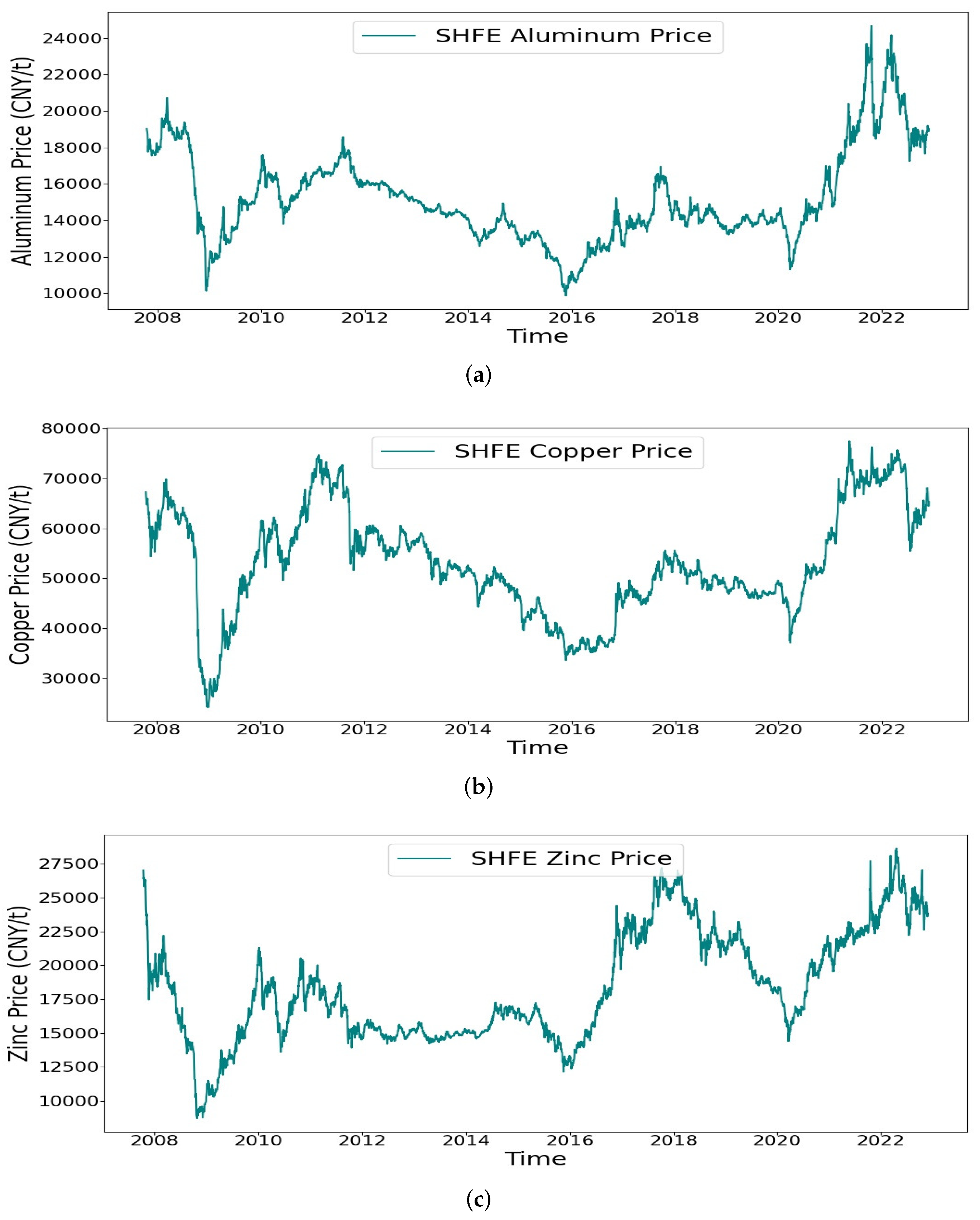
Metal materials have a large share of the Chinese market, and it is of great significance to research their price changes. The Shanghai Futures Exchange (SHFE) is an influential future trading platform in the world, and we select three main price fluctuations of non-ferrous metals from SHFE, including aluminum, copper, and zinc, to test the stability of the established model. They are acquired from website https://market.cnal.com/historical/, accessed on 4 July 2023. Each dataset contains 3677 data points, corresponding to the time span from 16 October 2007 to 25 November 2022, and the close price is taken as the market price. Due to the particularity of Chinese market, the three datasets are violent swings in the time dimension, as seen in Figure 3.

4.2. Evaluation Criteria of Performance

We employ four commonly used prediction error measures including Root Mean Square Error (RMSE), Mean Absolute Error (MAE), Mean Absolute Percentage Error (MAPE) and determination coefficient $R^2$ to assess the effectiveness of proposed model. The following formulas is calculation about the three main indicators:

$$\begin{array}{c}\hfill RMSE=\sqrt{\frac{1}{I_{test}}\sum _{i=1}^{I_{test}}{(\widehat{y_i}-y_i)}^2}\end{array}$$

(31)

$$\begin{array}{c}\hfill MAE=\frac{1}{I_{test}}\sum _{i=1}^{I_{test}}|\widehat{y_i}-y_i|\end{array}$$

(32)

$$\begin{array}{c}\hfill MAPE=\frac{1}{I_{test}}\sum _{i=1}^{I_{test}}\left|\frac{\widehat{y_i}-y_i}{\widehat{y_i}}\right|\times 100\%\end{array}$$

(33)

$$\begin{array}{c}\hfill R^2=1-\frac{{\sum }_{i=1}^{I_{test}}{(\widehat{y_i}-y_i)}^2}{{\sum }_{i=1}^{I_{test}}{(\widehat{y_i}-\overline{y_i})}^2}\end{array}$$

(34)

where $I_{tset}$ denotes the number of the validation set; $y_i$, $\overline{y_i}$ and $\widehat{y_i}$ are the raw value, average value and predicted value, respectively. The MAE, MAPE and RMSE are used to assess the proximity of the forecast data to the actual data, and the lower the three indicators is, the more reliable the trained model is. The closer $R^2$ is to 1, the better the model performs.

4.3. Related Parameters

The parameters are crucial for the model, although its acquisition process consumes much computational resources and time. Fundamentally, the batch size is firstly determined to be 16; the initial epoch is 100. On trial, neurons in each hidden layer are within [16, 128] interval, learning rate and decay rate are both within [0.00001, 0.01] interval. The number of the hidden layer is set as 1; other hyperparameters of the LSTM network are optimized by the SSO algorithm. In the end, the number of hidden neurons is 32, learning rate for IMF1 is 0.0001, while learning rate for other IMFs is 0.01. For the fairness of comparison, other models are also set with the same hyperparameters. The related and important parameters are shown in

Table 1. Related parameters and description.

Related Parameters	Value	Description
Validation split	0.1	The proportion of a training set used to validate during training.
Shuffle	True	Whether to randomly disrupt the order of input samples during training.
Epochs	100	How many times that a complete dataset passes the neural network once and returns during training.
Batch size	16	The number of samples contained in each batch when performing gradient descent.
Cells	32	The number of neurons in the hidden layer.
Activation	SeLU	The activation function for connected layer.
Optimizer	Nadam	The optimization method, here its loss is MSE.
Callbacks	/	ReduceLROnPlateau and EarlyStopping mechanisms of Keras are used for improvement.
Patience	20,30	The epochs for the model to perform the callbacks operations, one-tenth of the total epochs for reducing learning rate and a half for the early stop.

.

For the first stage of CEEMDAN treatment, the relevant parameters is referred to literature [25,29]. Where amplitude of the white Gaussian noise is 0.2, the number of trials is 100. Furthermore, the parameters of SE are referred to literature [30], m is set to 2, the similarity tolerance $r=0.2SD$. For the second stage of the decomposition, the window length of SSA is 21.

4.4. Empirical Results and Analysis

4.4.1. Multivariate Mode Decomposition Results

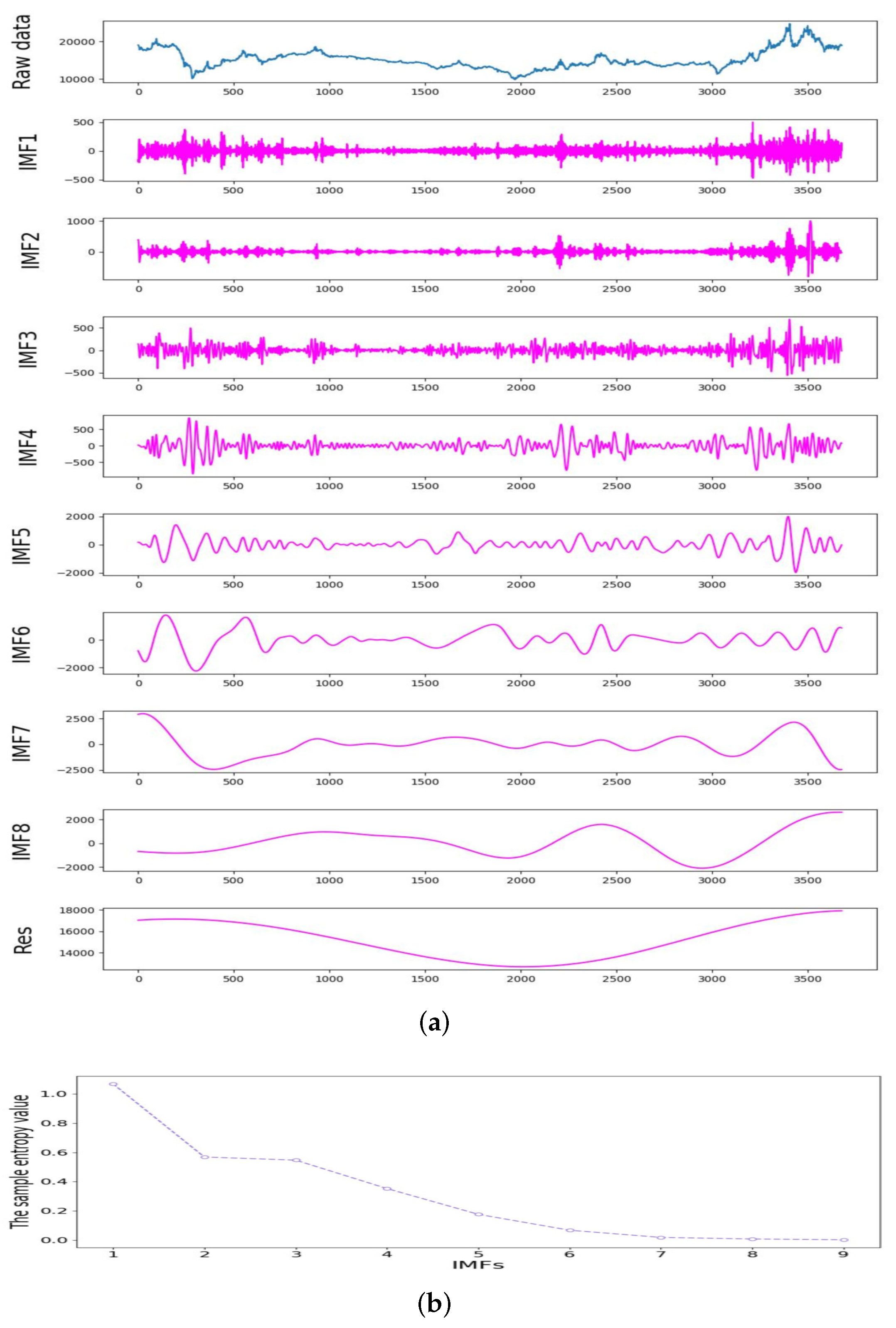
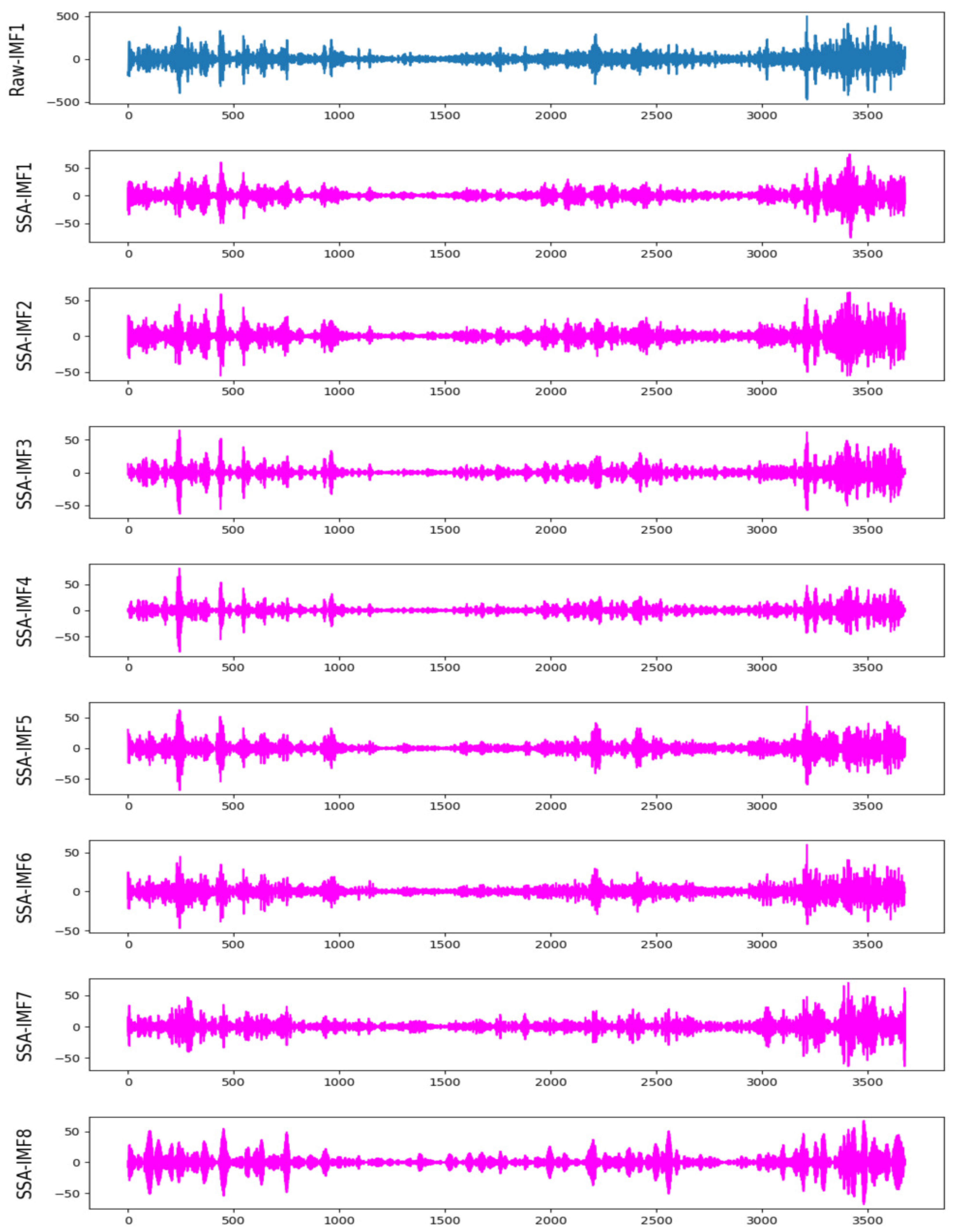
In the case of aluminum price, the Figure 4a shows the treatment results of CEEMDAN, including eight IMFs and one residual. The residual component of low frequency approximately represents the trend of price, while the other components contain the details or differences of the original signal. Relatively speaking, the subsequences become smoother, but the high-frequency subsequences still fluctuate sharply, consistent with the SE results in Figure 4b. According to Figure 4b, in order not to waste computing resources, the six components with small sample entropy are integrated into Combined Intrinsic Mode Functions (Co-IMFs), namely Co-IMF4 (IMF4, IMF5, IMF6, IMF7, IMF8 and Res). Its sample entropy is 0.0432. What’s more, IMF1 has the largest SE, indicating that it has the most complex structure. As seen Figure 5, IMF1 is decomposed by the SSA method into 8 components. Further decomposition and the combination can reduce the complexity of the original series, which is conducive to mining the change law.

4.4.2. Analysis of Forecast Results

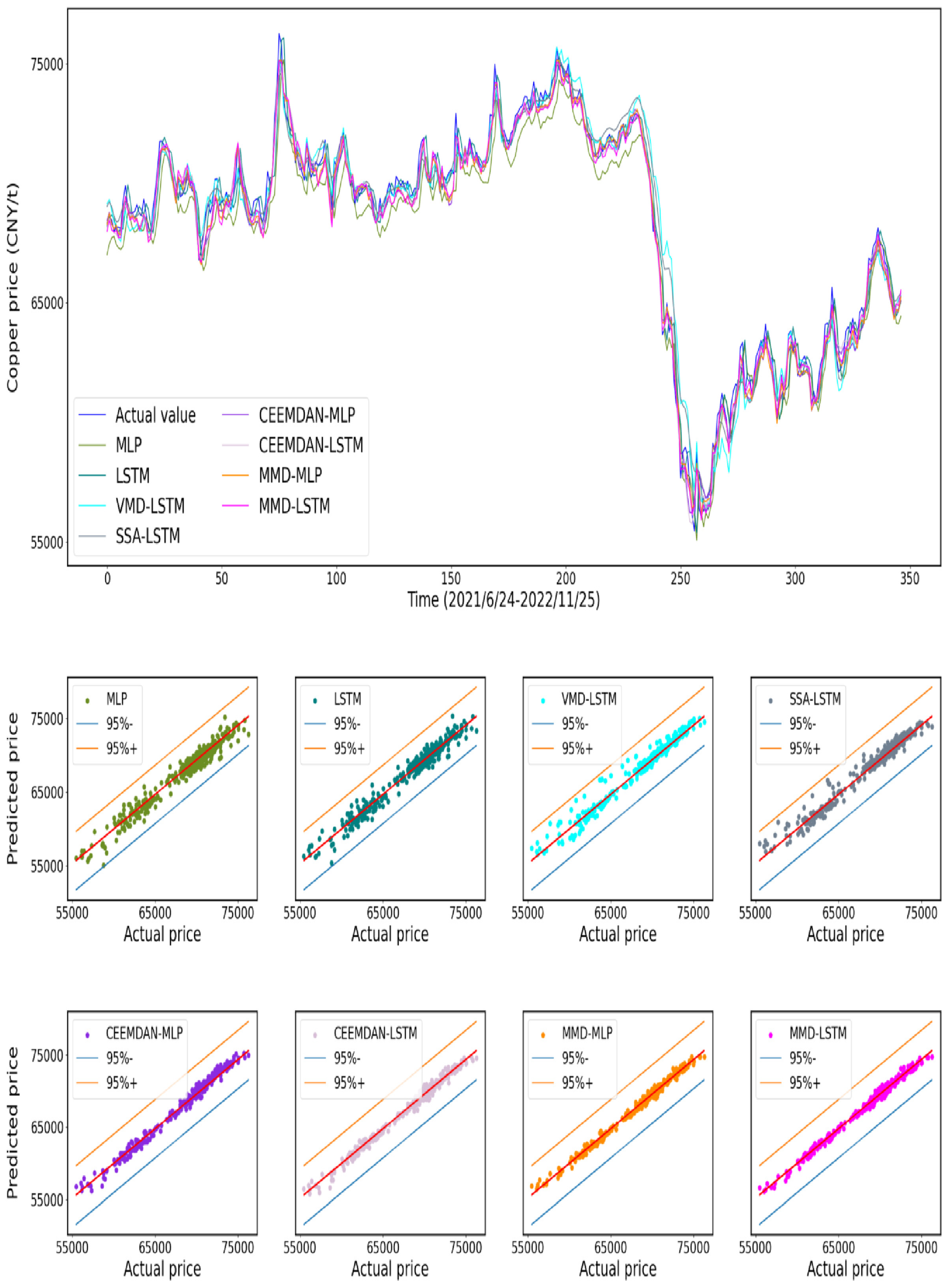
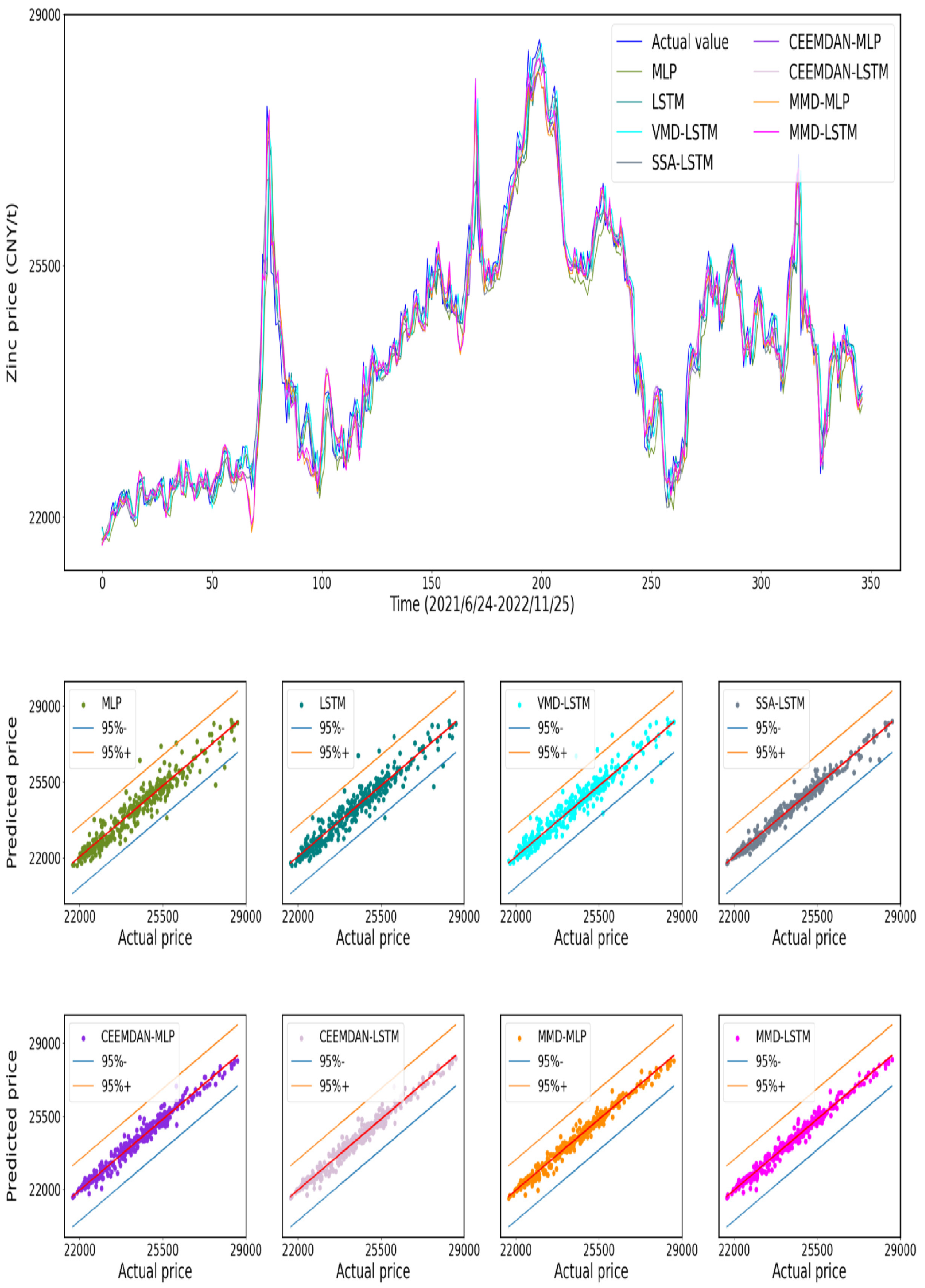
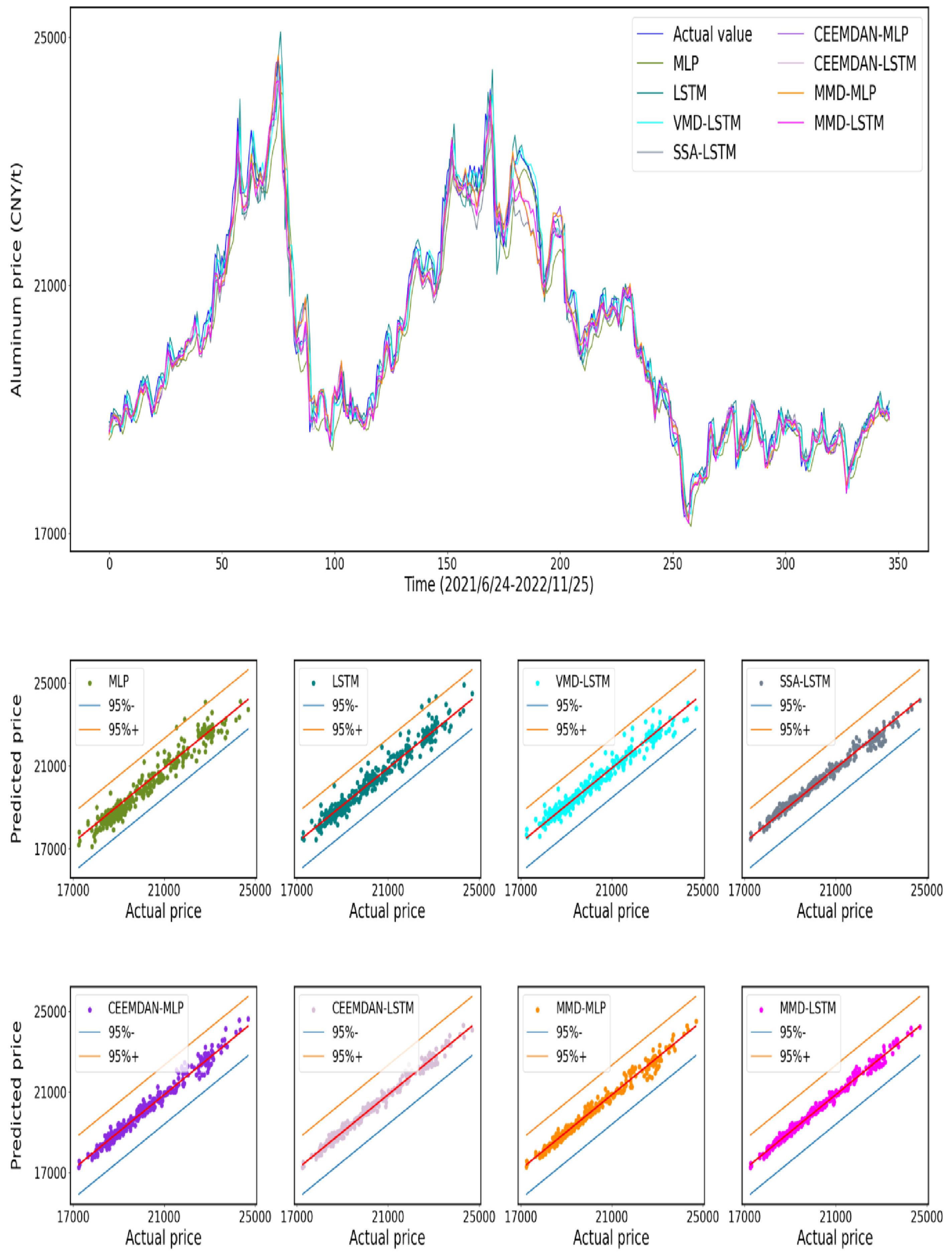
After obtaining the smooth data, we employ various neural network models to learn the laws of historical data, with the prediction schemes being: MLP, LSTM, VMD-LSTM, SSA-LSTM, CEEMDAN-MLP, CEEMDAN-LSTM, MMD-MLP, and MMD-LSTM. To validate the validity of the proposed model, it is compared with seven benchmark models from different angles. Figure 6, Figure A1 and Figure A2 illustrate the comparison graphs and scatter graphs, which visually show the accuracy of various models to forecast non-ferrous metals price.

In the first place, take the aluminum price as an example, the proximity between the predicted and actual values is demonstrated by viewability, as shown in Figure 6. According to the top error comparison graph, the error trend is gradually decreasing; both MMD-LSTM, MMD-MLP and CEEMDAN-LSTM model have the smaller error and the smaller fluctuation range. The scatter plots below mainly present the scattered observation values obtained from linear fitting of the predicted values, and the confidence intervals are used to evaluate the prediction performance [2,18,39,40]. Drawing a scatter plot of the following eight models, it can be seen that comparing the proposed model with the other seven models. It pointed out that the proposed model focuses on the linear fitting line and has the narrowest 95% forecast band. It indicates the 95% forecast band of fusion models are better than single models, and the forecast band of MMD-LSTM is clearly better than VMD-LSTM, SSA-LSTM, CEEMDAN-MLP, and MMD-MLP. These conclusions demonstrate that the choice of LSTM and MMD is proper.

In the second place, While the complex nonlinear price series are decomposed into several subsequences by the CEEMDAN algorithm, the fluctuation characteristics become more obvious, reducing the complexity of the original price sequence. As a result, the CEEMDAN-class method can significantly improve the prediction performance, compared to the single model. Further, if the high-frequency subsequences continue to be decomposed by SSA, the prediction accuracy is improved again. This means that the MMD algorithm facilitates the mining of underlying regularities about price sequence.

Last but not least, quantitative analyses are performed, and the RMSE, MAE, MAPE, and $R^2$ for each method on the three datasets are shown in

Table 2. The metrics of various models for aluminum price forecast.

Models	RMSE	MAE	MAPE(%)	${\mathit{R}}^2$
MLP	405.5379	312.0251	1.5204	0.9415
LSTM	362.5705	258.0344	1.2651	0.9532
VMD-LSTM	317.6078	223.8584	1.1006	0.9641
SSA-LSTM	280.2321	198.3769	0.9435	0.9721
CEEMDAN-MLP	244.8113	184.1368	0.8947	0.9786
CEEMDAN-LSTM	219.5632	163.7091	0.7903	0.9828
MMD-MLP	223.7218	164.3561	0.7953	0.9822
MMD-LSTM	195.6278	141.2734	0.6779	0.9863

and

Table A1. The metrics of non-ferrous metals price forecast by various models.

Metals	Models	RMSE	MAE	MAPE(%)	${\mathit{R}}^2$
Copper	MLP	1111.9553	903.2919	1.3233	0.9389
	LSTM	836.6295	633.7231	0.9452	0.9654
	VMD-LSTM	740.8218	555.5603	0.8238	0.9665
	SSA-LSTM	764.3102	545.408	0.8217	0.9711
	CEEMDAN-MLP	537.9811	423.3759	0.6307	0.9856
	CEEMDAN-LSTM	524.3169	411.9391	0.6101	0.9864
	MMD-MLP	443.2475	357.9791	0.5306	0.9902
	MMD-LSTM	435.5633	352.4775	0.5167	0.9906
Zinc	MLP	463.8865	334.9679	1.3571	0.9127
	LSTM	429.8289	299.0934	1.2194	0.9251
	VMD-LSTM	407.9518	282.3788	1.1504	0.9325
	SSA-LSTM	256.5028	189.0633	0.7684	0.9733
	CEEMDAN-MLP	268.7251	204.0592	0.8297	0.9707
	CEEMDAN-LSTM	250.2042	188.0501	0.7693	0.9746
	MMD-MLP	239.2537	181.464	0.7374	0.9767
	MMD-LSTM	209.4423	153.0592	0.6266	0.9822

. In the case of aluminum price, from Table 2, the RMSE, MAE, MAPE, and $R^2$ of LSTM are 362.5705, 358.0344, 1.2651% and 0.9532, which are significantly better than MLP. This is attributed to its ability to capture the long-term dependence of the price sequence through the gate mechanism, while the single model cannot effectively extract features from complex price sequences. The RMSE, MAE, and MAPE of VMD-LSTM, SSA-LSTM, CEEMDAN-LSTM and MMD-LSTM are smaller than LSTM, which indicates that the decomposition algorithm can reduce the interference of Gaussian noise and improve the prediction performance. This is to say, the fusion model can efficiently extract main features from trend and detail components, thus alleviating the forecast difficulty caused by complex original series. Additionally, in terms of MMD-LSTM, the RMSE, MAE, MAPE and $R^2$ are 195.6278, 141.2734, 0.6779%, and 0.9863, concretely. Furthermore, the RMSE, MAE, and MAPE compared with MMD-MLP are respectively decreased by 12.5576%, 14.0443%, and 14.7617% at least; comparing with LSTM are respectively decreased by 46.0442%, 45.2502%, and 46.4153% at least. From among VMD-LSTM, SSA-LSTM, CEEMDAN-LSTM and MMD-LSTM, obviously, the MMD-LSTM has higher prediction accuracy. This is ascribed to the fact that the dual-stage processing using the MMD method reduces the complexity of the original sequence.

4.4.3. Analysis of Statistics

Aiming to explore the predictive performance of the various methods, Wilcoxon signed-rank test is used to validate whether there are significant differences between these methods [11,41]. Here, the significance level is 5%, and the control group is the MMD-LSTM method. The statistical results for Wilcoxon signed-rank test are shown in

Table 3. The Wilcoxon signed-rank test of aluminum price forecast.

Non-Ferrous Metals	Models	Wilcoxon Signed-Rank Test
		W = 100	p-Value
Aluminum	MLP	0	0.000000
	LSTM	0	0.000000
	VMD-LSTM	0	0.000002
	SSA-LSTM	48	0.00100
	CEEMDAN-MLP	22	0.000327
	CEEMDAN-LSTM	57	0.004319
	MMD-MLP	22	0.000131

and

Table A2. The Wilcoxon signed-rank test of non-ferrous metals price forecast.

Non-Ferrous Metals	Models	Wilcoxon Signed-Rank Test
		W = 100	p-Value
Copper	MLP	0	0.000000
	LSTM	0	0.000002
	VMD-LSTM	22	0.000372
	SSA-LSTM	43	0.000905
	CEEMDAN-MLP	56	0.002495
	CEEMDAN-LSTM	81	0.008776
	MMD-MLP	134	0.077883
Zinc	MLP	0	0.000000
	LSTM	73	0.007916
	VMD-LSTM	56	0.002537
	SSA-LSTM	15	0.000153
	CEEMDAN-MLP	0	0.000000
	CEEMDAN-LSTM	57	0.004081
	MMD-MLP	23	0.000420

. Where the p-value is the probability that more extreme results than the resulting observed sample will appear when the null hypothesis is true. The smaller p-value, the more sufficient justification for the null hypothesis being rejected. According to the statistical results from Table 3, the p-value of these benchmark models is less than 5%, which means that the prediction performance of the proposed method is significantly different from MLP, LSTM, VMD-LSTM, SSA-LSTM, CEEMDAN-MLP, CEEMDAN-LSTM, and MMD-MLP. These conclusions demonstrate the feasibility of the proposed dual-stage MMD algorithm in the non-ferrous metals price forecast.

5. Conclusions

The forecast of non-ferrous metals prices is significant for establishing a practical and stable pricing mechanism and providing practical guidance for production, operation, and investment. In this work, we have proposed a novel fusion model based on CEEMDAN, SSA, and LSTM, namely MMD-LSTM. To validate the prediction performance of the proposed model, test experiments were performed on historical data of aluminum, copper, and zinc from SHFE and compared with MLP, LSTM, VMD-LSTM, SSA-LSTM, CEEMDAN-MLP, CEEMDAN-LSTM, and MMD-MLP. The qualitative and quantitative analysis results show that the proposed MMD-LSTM model is a better prediction framework. Compared with single models, the fusion model based on the decomposition algorithm has higher prediction accuracy, which denotes that the signal decomposition is beneficial to fully grasp the features of the raw sequence. Even more, the prediction models based on VMD, SSA, or CEEMDAN algorithm, have made great progress in recent years. Nevertheless, the proposed dual-stage processing using the MMD algorithm can reduce the complexity of high-frequency sequences and has higher prediction accuracy. Because the proposed MMD-LSTM method has taken the irregularities of non-ferrous metals price sequence into account, it could provide some meaningful references for the industry.

6. Future Work

The proposed prediction method performs well in non-ferrous metals price forecasts. However, it is noteworthy that although the dual-stage decomposition algorithm is beneficial in reducing the complexity of the original sequence, substantial computational resources are consumed. In addition, the MMD-LSTM method is not processed by a parallel algorithm in this paper, and the computational efficiency is greatly reduced. Therefore, to save computing resources and improve prediction performance, we will further optimize the prediction model by combining a more feasible decomposition algorithm with the state-of-the-art network in future work.

References

1. Ron, A.; Bhattarai, S.; Coibion, O. Commodity-price comovement and global economic activity. J. Monet. Econ. 2020, 112, 41–56. [Google Scholar]
2. Gil, C. Algorithmic Strategies for Precious Metals Price Forecasting. Mathematics 2022, 10, 1134. [Google Scholar]
3. Garcĺa, D.; Kristjanpoller, W. An adaptive forecasting approach for copper price volatility through hybrid and non-hybrid models. Appl. Soft Comput. 2019, 74, 466–478. [Google Scholar] [CrossRef]
4. Gillian, D.; Lenihan, H. An assessment of time series methods in metal price forecasting. Resour. Policy 2005, 30, 208–217. [Google Scholar]
5. Sungdo, K.; Min, M.B.; Joo, B.S. Data depth based support vector machines for predicting corporate bankruptcy. Appl. Intell. 2018, 48, 791–804. [Google Scholar]
6. Yusheng, H.; Gao, Y.; Gan, Y.; Ye, M. A new financial data forecasting model using genetic algorithm and long short-term memory network. Neurocomputing 2021, 425, 207–218. [Google Scholar]
7. Yunlei, Y.; Yang, W.; Muzhou, H.; Lou, J.; Xie, X. Solving Emden-Fowler Equations Using Improved Extreme Learning Machine Algorithm Based on Block Legendre Basis Neural Network. Neural Process. Lett. 2023, 1–20. [Google Scholar]
8. Liu, C.; Hu, Z.; Li, Y.; Liu, S. Forecasting copper prices by decision tree learning. Resour. Policy 2017, 52, 427–434. [Google Scholar] [CrossRef]
9. Pinyi, Z.; Ci, B. Deep belief network for gold price forecasting. Resour. Policy 2020, 69, 101806. [Google Scholar]
10. Chen, Y.; Wang, D.; Kai, C.; Pan, C.; Yu, Y.; Hou, M. Prediction of safety parameters of pressurized water reactor based on feature fusion neural network. Ann. Nucl. Energy 2022, 166, 108803. [Google Scholar] [CrossRef]
11. Liu, Q.; Liu, M.; Zhou, H.; Yan, F. A multi-model fusion based non-ferrous metal price forecasting. Resour. Policy 2022, 77, 102714. [Google Scholar] [CrossRef]
12. Dehghani, H.; Bogdanovic, D. Copper price estimation using bat algorithm. Resour. Policy 2018, 55, 55–61. [Google Scholar] [CrossRef]
13. Bilin, S.; Maolin, L.; Yu, Z.; Genqing, B. Nickel Price Forecast Based on the LSTM Neural Network Optimized by the Improved PSO Algorithm. Math. Probl. Eng. 2019, 2019, 1934796. [Google Scholar]
14. Roslindar, Y.S.; Zakaria, R. ARIMA and Symmetric GARCH-type Models in Forecasting Malaysia Gold Price. J. Phys. Conf. Ser. 2019, 1366, 012126. [Google Scholar]
15. Hou, M.; Liu, T.; Yang, Y.; Hao, Z.; Hongjuan, L.; Xiugui, Y.; Xinge, L. A new hybrid constructive neural network method for impacting and its application on tungsten price prediction. Appl. Intell. 2017, 47, 28–43. [Google Scholar]
16. Andrés, V.; Werner, K. Gold Volatility Prediction using a CNN-LSTM approach. Expert Syst. Appl. 2020, 157, 113481. [Google Scholar]
17. Hu, Y.; Ni, J.; Wen, L. A hybrid deep learning approach by integrating LSTM-ANN networks with GARCH model for copper price volatility prediction. Phys. A Stat. Mech. Its Appl. 2020, 557, 124907. [Google Scholar] [CrossRef]
18. Chu, Z.; Muhammad, S.N.; Tian, P.; Hua, L.; Ji, C. An evolutionary robust solar radiation prediction model based on WT-CEEMDAN and IASO-optimized outlier robust extreme learning machine. Appl. Energy 2022, 322, 119518. [Google Scholar]
19. Wang, J.; Li, X. A combined neural network model for commodity price forecasting with SSA. Soft Comput. 2018, 22, 5323–5333. [Google Scholar] [CrossRef]
20. Zhou, S.; Lai, K.K.; Yen, J. A dynamic meta-learning rate-based model for gold market forecasting. Expert Syst. Appl. 2012, 39, 6168–6173. [Google Scholar] [CrossRef]
21. Ming, L.; Yang, S.; Cheng, C. The double nature of the price of gold-A quantitative analysis based on Ensemble Empirical Mode Decomposition. Resour. Policy 2016, 47, 125–131. [Google Scholar] [CrossRef]
22. Wen, F.; Yang, X.; Gong, X.; Lai, K.K. Multi-Scale Volatility Feature Analysis and Prediction of Gold Price. Int. J. Inf. Technol. Decis. Mak. 2017, 16, 205–223. [Google Scholar] [CrossRef]
23. Lahmiri, S. Long memory in international financial markets trends and short movements during 2008 financial crisis based on variational mode decomposition and detrended fluctuation analysis. Phys. A Stat. Mech. Its Appl. 2015, 437, 130–138. [Google Scholar] [CrossRef]
24. Liu, Y.; Yang, C.; Huang, K.; Gui, W. Non-ferrous metals price forecasting based on variational mode decomposition and LSTM network. Knowl. Based Syst. 2019, 188, 105006. [Google Scholar] [CrossRef]
25. Feite, Z.; Zhehao, H.; Changhong, Z. Carbon price forecasting based on CEEMDAN and LSTM. Appl. Energy 2022, 311, 118601. [Google Scholar]
26. Wei, S.; Wang, X.; Tan, B. Multi-step wind speed forecasting based on a hybrid decomposition technique and an improved back-propagation neural network. Environ. Sci. Pollut. Res. 2022, 49, 684–699. [Google Scholar]
27. Zhaohua, W.; Huang, N.E. Ensemble empirical mode decomposition: A noise-assisted data analysis method. Adv. Adapt. Data Anal. 2009, 1, 1–41. [Google Scholar]
28. Yeh, J.-R.; Shieh, J.-S.; Huang, N.E. Complementary ensemble empirical mode decom-position: A novel noise enhanced data analysis method. Adv. Adapt. Data Anal. 2010, 2, 135–156. [Google Scholar] [CrossRef]
29. Colominas, M.A.; Schlotthauer, G.; Torres, M.E. Improved complete ensemble EMD: A suitable tool for biomedical signal processing. Biomed. Signal Process. Control 2014, 14, 19–29. [Google Scholar] [CrossRef]
30. Richman, J.S.; Moorman, J.R. Physiological time-series analysis using approximate entropy and sample entropy. Am. J. Physiol. Heart Circ. Physiol. 2000, 278, H2039–H2049. [Google Scholar] [CrossRef]
31. Peng, D.; Xiu, N.; Yu, J. Global Optimality Condition and Fixed Point Continuation Algorithm for Non-Lipschitz lp Regularized Matrix Minimization. Sci. China Math. 2018, 61, 1139–1152. [Google Scholar] [CrossRef]
32. Yan, X.; Weihan, W.; Chang, M. Research on financial assets transaction prediction model based on LSTM neural network. Neural. Comput. Appl. 2020, 33, 257–270. [Google Scholar] [CrossRef]
33. Cao, X.; Fekan, M.; Shen, D.; Wang, J. Iterative learning control for multi-agent systems with impulsive consensus tracking. Nonlinear Anal. Model. 2021, 26, 130–150. [Google Scholar] [CrossRef]
34. Yu, C.; Zhao, Y.; Qi, X.; Ma, H.; Wang, C. LLR: Learning learning rates by LSTM for training neural networks. Neurocomputing 2020, 394, 41–50. [Google Scholar] [CrossRef]
35. He, Q.; Wang, Y. Reparameterized full-waveform inversion using deep neural networks. Geophysics 2021, 86, 1–13. [Google Scholar] [CrossRef]
36. Xue, J.; Shen, B. A novel swarm intelligence optimization approach: Sparrow search algorithm. Syst. Sci. Control. Eng. 2020, 8, 22–34. [Google Scholar] [CrossRef]
37. Hochreiter, S.; Schmidhuber, J. Long short-term memory. Neural Comput. 1997, 9, 1735–1780. [Google Scholar] [CrossRef]
38. Li, Y.; Fan, C.; Li, Y.; Wu, Q.; Ming, Y. Improving deep neural network with multiple parametric exponential linear units. Neurocomputing 2018, 301, 11–24. [Google Scholar] [CrossRef]
39. Hou, M.; Lv, W.; Kong, M.; Li, R.; Liu, Z.; Wang, D.; Wang, J.; Chen, Y. Efficient predictor of pressurized water reactor safety parameters by topological information embedded convolutional neural network. Ann. Nucl. Energy. 2023, 192, 110004. [Google Scholar] [CrossRef]
40. Xia, Y.; Wang, J.; Zhang, Z.; Wei, D.; Yin, L. Short-term PV power forecasting based on time series expansion and high-order fuzzy cognitive maps. Appl. Soft Comput. 2023, 135, 110037. [Google Scholar] [CrossRef]
41. Li, M.-W.; Xu, D.-Y.; Jing, G.; Hong, W.-C. A hybrid approach for forecasting ship motion using CNN-GRU-AM and GCWOA. Appl. Soft Comput. 2022, 114, 108084. [Google Scholar] [CrossRef]
Figure 1. The overall structure of LSTM network.
Axioms 12 00670 g001
Figure 2. The whole prediction flow of metals price forecast by LSTM model.
Axioms 12 00670 g002
Figure 3. The non-ferrous metals price on SHFE from 16 October 2007 to 25 November 2022. (a) Aluminum futures price. (b) Copper futures price. (c) Zinc futures price.
Axioms 12 00670 g003
Figure 4. The decomposition result of SHFE aluminum price. (a) demonstrates the first stage decomposition result by CEEMDAN, (b) shows the sample entropy value of each subsequence.
Axioms 12 00670 g004
Figure 5. The second stage decomposition result of IMF1 by SSA.
Axioms 12 00670 g005
Figure 6. The forecast result of aluminum price.
Axioms 12 00670 g006