A Fuzzy-Random Extension of Jamshidian’s Bond Option Pricing Model and Compatible One-Factor Term Structure Models

Abstract

The primary objective of this paper is to expand Jamshidian’s bond option formula and compatible one-factor term structure models by incorporating the existence of uncertainty in the parameters governing interest-rate fluctuations. Specifically, we consider imprecision in the parameters related to the speed of reversion, equilibrium short-term interest rate, and volatility. To model this uncertainty, we utilize fuzzy numbers, which, in this context, are interpreted as epistemic fuzzy sets. The second objective of this study is to propose a methodology for estimating these parameters based on historical data. To do so, we use the possibility distribution functions capability to quantify imprecise probability distributions. Furthermore, this paper presents an application to the term structure of fixed-income bonds with the highest credit rating in the Euro area. This empirical application allows for evaluating the effectiveness of the fuzzy extension in fitting the dynamics of interest rates and assessing the suitability of the proposed extension.

1. Introduction

The Black–Scholes–Merton option pricing model (referred to as BSM) introduced by Black and Scholes [1] and Merton [2] is widely recognized as a cornerstone in the field of option pricing and financial economics [3]. The value of the BSM model can be seen from two perspectives. First, from a narrow viewpoint of option pricing, the BSM model provides an operational formula. Second, from a broader asset pricing context, the “arbitrage argument” generalized by the concepts of “risk-neutral valuation” offers a powerful framework. This framework allows for determining the price of any contingent asset as the expected present value of promised cash flows [4].

The analytical framework initiated by the BSM model has been particularly fruitful in modeling the term structure of interest rates, as it has generated a wide range of models that have been applied to the evaluation of yield-curve dynamics and bond valuation, as well as the valuation of derivative assets on interest-rate-sensitive instruments such as bond options, caps, or floors. Following Sundaresan [5], we can distinguish three types of models: unifactorial, multifactorial, and calibrated, also known as variable parameter models [6].

• Unifactorial models fit the term structure with solely the movement of short-term interest rates. Examples of such models are [7,8];
• Multifactorial models, developed toward the end of the 1970s, explain the dynamics of interest-rate movements using one or several additional factors, such as fluctuations in long-term interest rates, the spread between short- and long-term interest rates, or volatility. An example of this approach is [9];
• The parsimony of the models discussed above allows them to be useful for a wide range of economic and financial analyses, such as testing the existence of mean reversion in prices and modeling discount rates for financial and actuarial pricing. Likewise, their estimation has a low cost since it requires the adjustment of a few parameters. On the other hand, that parsimony leads them to have a limited ability to capture the profiles of the term structure of interest rates, thus limiting their usefulness in other applications such as valuing derivative assets [6]. This problem gave rise in the late 1980s to models called calibrated or time-varying parameter models [10,11,12,13]. These are unifactorial models that model the fluctuation of short-term interest rates in a manner similar to [7] but allow for variability in the parameters of the stochastic process, which are calibrated with zero-coupon bond prices to perfectly capture the observed yield curve. While such models are widely used in derivative asset valuation, their lack of parsimony reduces their interest in other types of analysis.

Option pricing models have relied on the analytical framework of stochastic calculus and probability theory since their inception [14]. Nevertheless, financial and economic activity involves varying degrees of knowledge and may combine risk with other sources of uncertainty, such as imprecision or vagueness. Fuzzy-subset theory is a valid tool for modeling uncertainty, and fuzzy numbers can be used for this same purpose regarding a variable. For example, for a reference ${\mathbb{R}}^{+}$ and a variable ${\sigma }_0$ (such as volatility), we can define the fuzzy number $\tilde{\sigma }$, which can be interpreted as “volatility is approximately $\tilde{\sigma }$” with the degree of possibility of σ$\in {\mathbb{R}}^{+}$ in $\tilde{\sigma }$ being the likelihood that this variable precisely takes the value σ [15].

The usefulness of fuzzy-subset theory has been exploited by various authors to model the uncertainty of the parameters that govern the random movement of the underlying asset in option pricing models. This stochastic process, which can be in discrete or continuous time, is fuzzified by modeling the uncertainty about the parameters that govern the evolution of the underlying asset prices, assuming that they are fuzzy numbers, defined through a possibility distribution [16]. This is a set of works that make up a current within fuzzy mathematics that can be categorized as fuzzy-random option pricing (FROP) [17]. A review of the FROP literature leads us to conclude that the type of random schemes in which the vagueness of the parameters is treated through fuzzy uncertainty is relatively broad. There is also a wide range of production in both equity and index options, as well as in real options [16]. However, the concern for connecting objective information from financial markets with the calibration of the parameters that make up the models has been much scarcer [16]. Moreover, the application of the FROP approach to fixed-income markets is practically nonexistent [17].

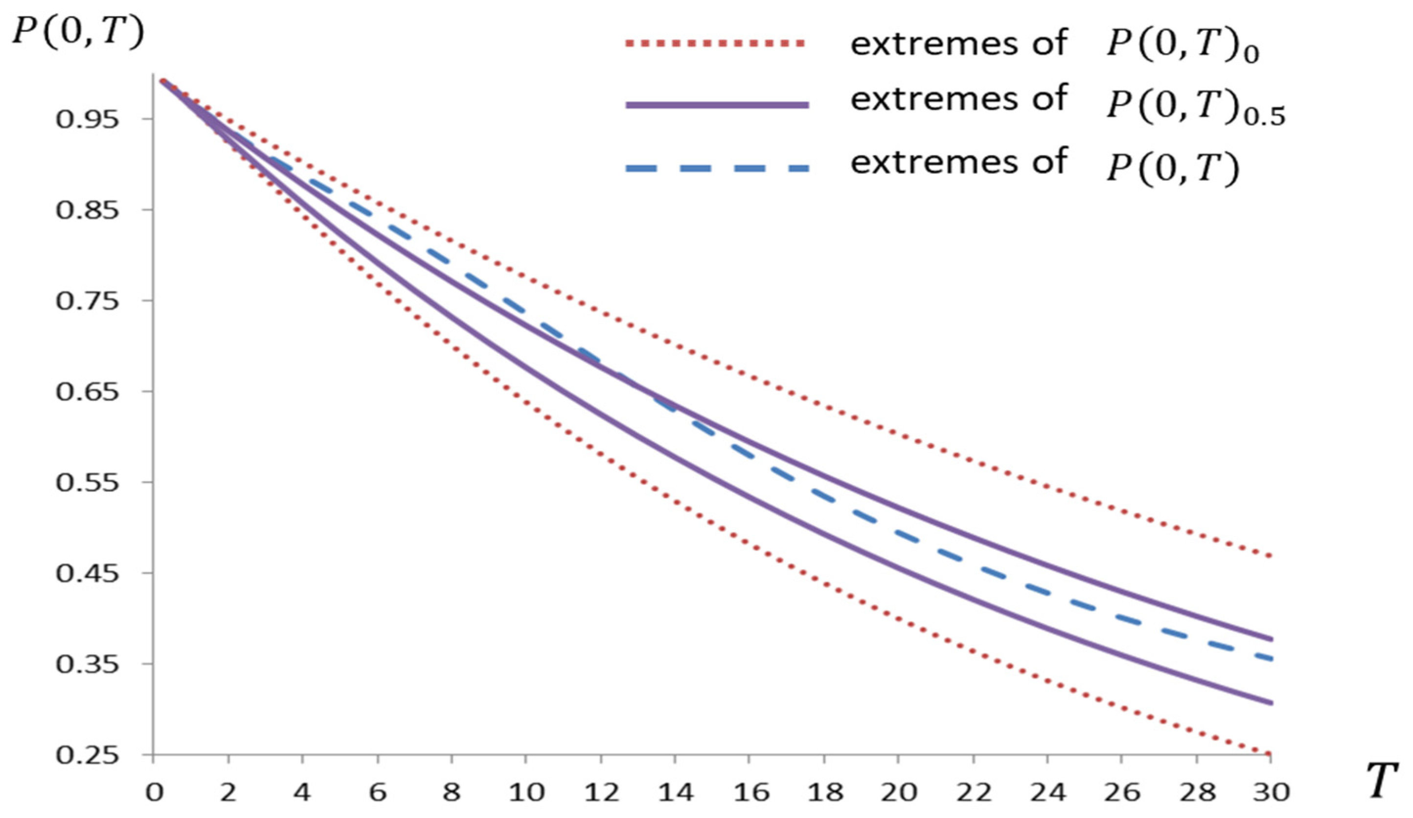
Thus, this paper aims to make a twofold contribution. The first would be motivated by the fact that the FROP literature is scarce in the context of fixed-income markets and the valuation of derivative instruments sensitive to interest rates. This work extends the term structure models compatible with bond option pricing by Jamshidian [18] and that option pricing formula to the assumption that the parameters governing the variation of short-term interest rates (equilibrium interest rate, speed of return to equilibrium, and market volatility) are imprecisely given through fuzzy numbers. Therefore, this paper extends the results in [19] about Vasicek’s model of term structure developed under the hypothesis that the parameters that rule short-term interest rates are given by fuzzy numbers.

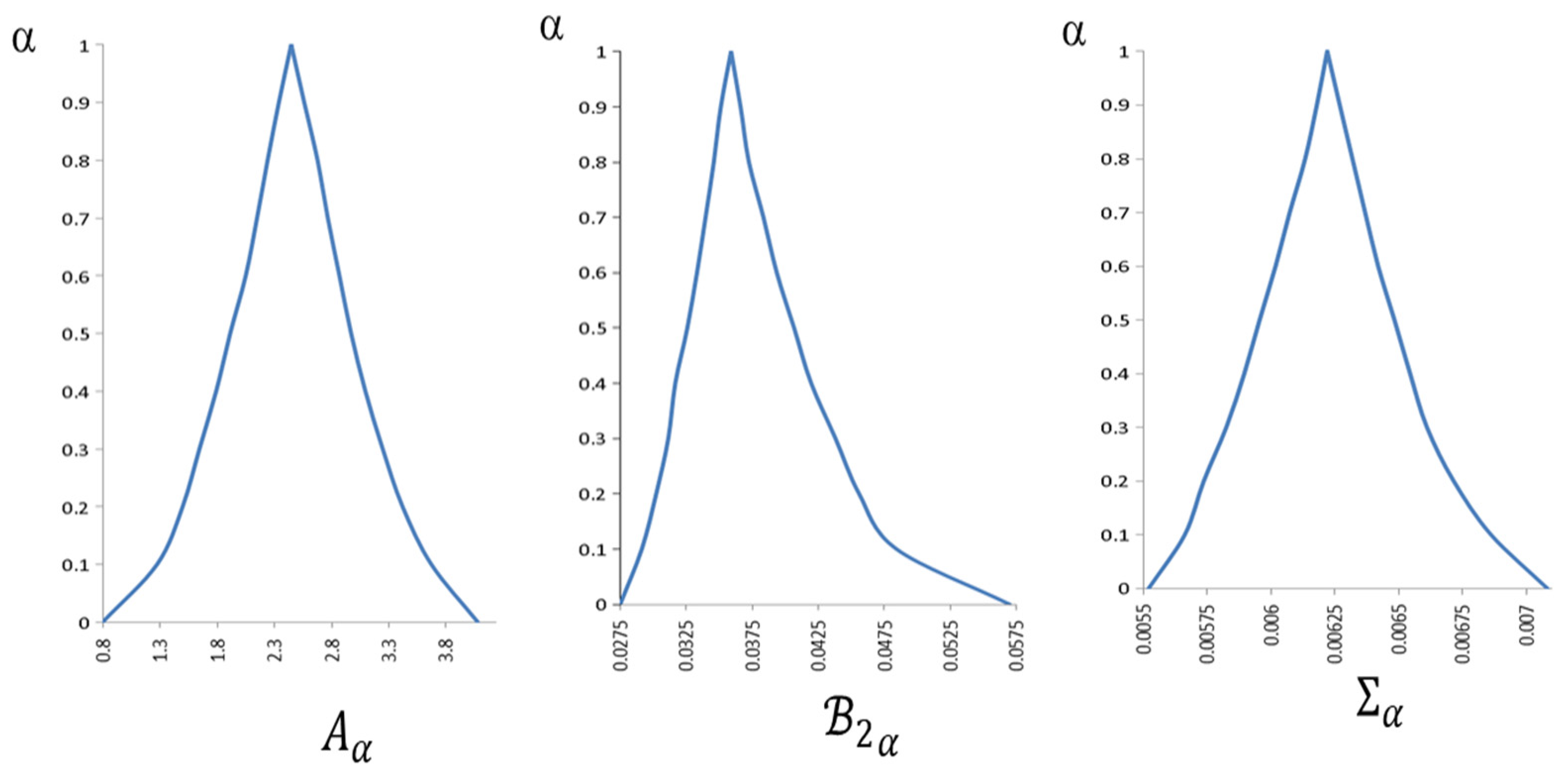
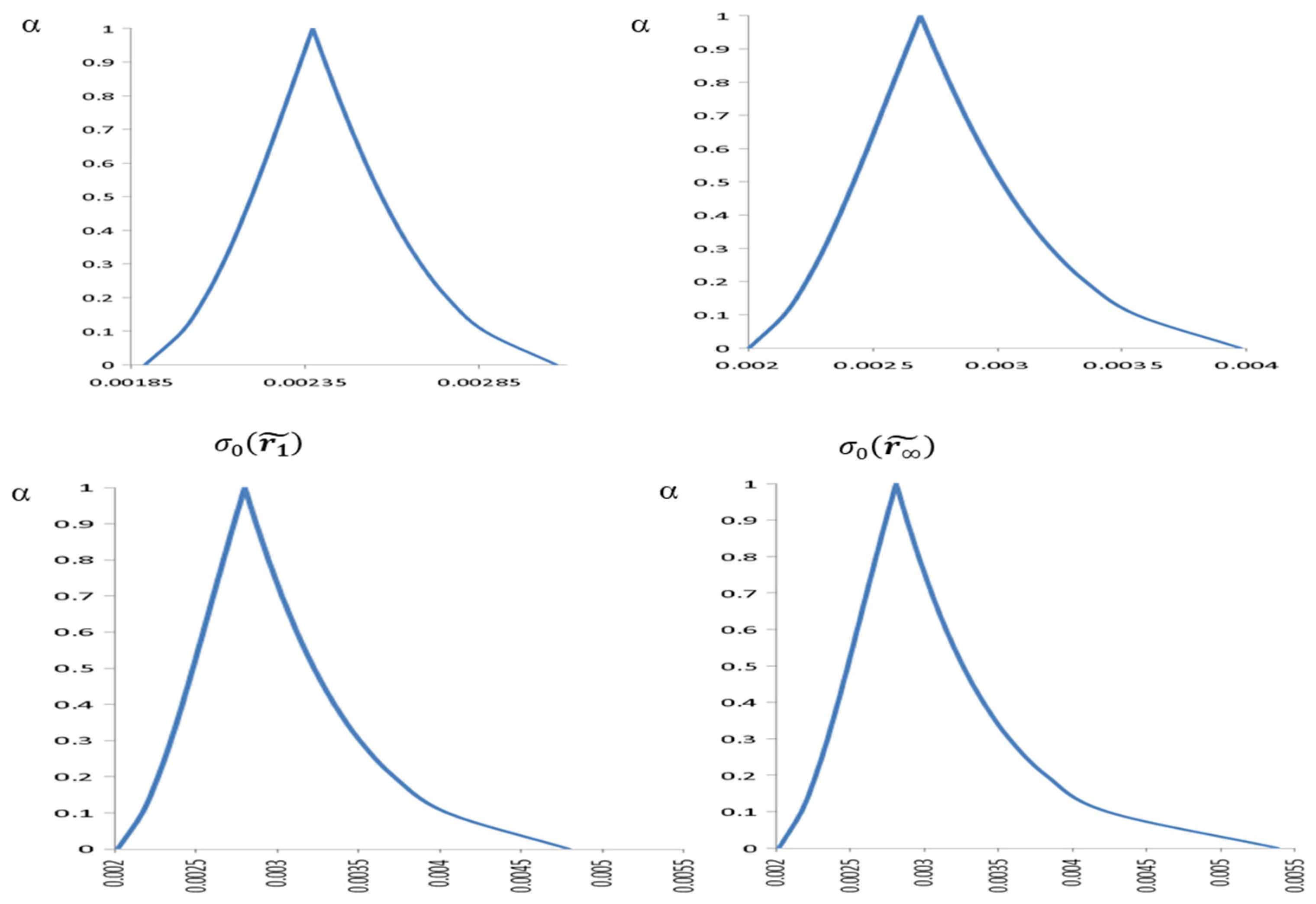
The second contribution of this work is to develop a methodology for estimating fuzzy parameters based on market data. On the one hand, we will take advantage of the fact that the α-cut of a fuzzy number can be interpreted as a confidence interval in which the probability that the variable of interest is $1-\alpha$ [20]. This allows us to use the approaches of [21,22,23], who propose quantifying estimates from conventional regression models through fuzzy numbers induced by statistical confidence intervals, and [24], who use an analogous procedure to model uncertainty of variance by using fuzzy numbers. 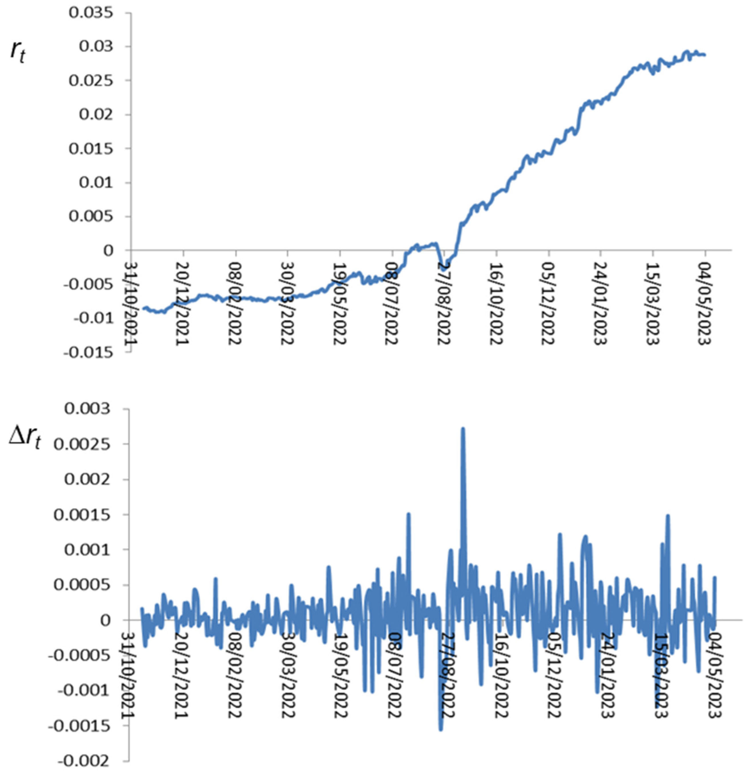On the other hand, those fuzzy estimates will be grounded in the standard parameter-calibration methodologies based on least-squares regression [6]. Our developments will be applied to data on the zero-coupon curve published by the European Central Bank for the highest credit-rated bonds in the Eurozone during the period from November 2021 to May 2023.

2. Fuzzy-Random Option Pricing

The fuzzy sets theory (FST) has provided tools that have been used in option pricing valuation to capture uncertainty as fuzzy measures, fuzzy numbers, fuzzy expert systems, or fuzzy regression [16,17]. These instruments have been intensively applied since the beginning of the 21st century to option valuation from four different perspectives [17]. The first perspective is what we have called FROP, with seminal works in this regard by [25,26,27]. This is the setting in which this paper must be understood. The second approach consists of using Sugeno’s integral and fuzzy measures to model the existence of imperfections in the market [28]. The third focus is the so-called fuzzy payoff for real options valuation [29]. The fourth approach seeks to take advantage of the ability of fuzzy neural networks as a universal function approximator to generate nonparametric option valuation models [30].

The mainstream in the literature on applications of fuzzy set theory to option pricing is likely the FROP approach [17]. These works assume that the fluctuations in underlying asset prices are governed by the hypothesis of a conventional option valuation model which, in continuous time, is often the geometric Brownian motion that underlies BSM and, in discrete time, the binomial framework by Cox, Ross, and Rubinstein [31]. In this approach, it is considered that the parameters of the stochastic process governing price fluctuations, such as volatility, are not crisp but are observed vaguely. A natural way to represent such uncertainty is through possibility distributions by means of fuzzy numbers [15]. Thus, the possibility function can be understood as an adequate approximation to the plausible values of the parameter of interest, while the degree of possibility of a value is interpreted as a physical measure of how easily that value will materialize in practice [15].

As an illustrative example of FROP, let us consider the random instantaneous fluctuations of the price of a financial asset, denoted as $\mathit{d}\mathit{S}$, which follows a geometric Brownian motion defined by the equation $\mathit{d}\mathit{S}=mSdt+\sigma S\mathit{d}\mathit{z}$. Here, $S$ represents the current price of the asset, $\mathit{d}\mathit{z}$ is a Gaussian random variable with a mean of zero and a standard deviation of $dt$, $m$ denotes the price annual growth rate, and $\sigma$ represents the annualized standard deviation of these fluctuations.

In the fuzzy-random approach, the precise values of the parameters m and σ are not known but are represented by fuzzy numbers $\tilde{m}$ and $\tilde{\sigma }$, respectively. The possibility distribution functions for $\tilde{m}$ and $\tilde{\sigma }$ are denoted as ${\mu }_m\left(x\right)$ and ${\mu }_{\sigma }\left(y\right)$, respectively. Consequently, the price fluctuation becomes a fuzzy-random variable and, for a possible random realization $\mathit{d}\mathit{S}=mSdt+\sigma S\mathit{d}\mathit{z}$, the possibility measure is $\mu \left(\mathit{d}\mathit{S}\right)=\min \left\{{\mu }_m\left(x\right),{\mu }_{\sigma }\left(y\right)\right\}$.

Regarding the framework utilized by FROP, contributions can be differentiated between discrete and continuous time. Developments in continuous time typically rely on conventional univariate geometric Brownian motion [25,26,27], which can be multivariate in the case of compound options [32]. However, the fuzzy-random literature has also extended to more complex continuous time modeling, such as Lévy processes [33,34] or fractional-type random movements [35,36,37,38]. In discrete time, the most common approach is provided by the binomial framework [31], with examples in this context found in [39,40,41,42,43]. Although less common, FROP has also employed other discrete time approximations, such as the trinomial methodology developed in [43] and Monte Carlo simulation [44].

The literature review of FROP in both continuous and discrete time leads to the conclusion that most works are devoted to the valuation of options on stocks or stock indices, either under the framework provided by the BSM model [26,45], other more sophisticated continuous time models [37,46], or using the binomial model as a reference [38,39,40].

Another particularly fertile field has been the valuation of real options, which has been carried out in continuous time with the framework provided by BSM [25] or with the derivative of the geometric diffusion models for multiple assets by Geske [47] or Margabre [48], [32,49]. In discrete time, we can mention the contributions [40,41,43,50,51,52]. Other applications of FROP to asset valuation include assessing firms’ values [27], as suggested by the seminal work [1], credit default swaps [53,54], bank deposit insurance [55], catastrophe bonds [56], and forward contracts in energy markets [57]. It is striking that FROP extensions to equilibrium models of the term structure or interest-rate derivative valuation models are scarce. In this sense, we can outline the extension of the [7] model of the yield curve in [19].

On the other hand, empirical applications that connect theoretical developments with objective market data are relatively scarce [16]. While [38] tests a fuzzy binomial extension on DAX index option data, ref. [58] proposes estimating the implied volatility of options using a probability–possibility transformation based on the empirical distribution function and [45,52] also use a probability–possibility transformation grounded on the confidence intervals of the underlying asset’s volatility that were obtained with inferential statistics mathematics.

3. One-Factor Equilibrium Term Models and Jamshidian’s Bond Option Pricing Formula

3.1. One-Factor Term Structure Models of Vasicek’s Type

In fixed-income markets, stochastic fluctuations of prices do not come directly from prices, as stated in option pricing models for stock markets, but due to fluctuations in the short-term rate r, which directly influences price fluctuations. In general, one-factor models suppose that r follows an Ito process [7]:

$$\mathit{d}\mathit{r}=m\left(r,t\right)dt+\mathsf{\sigma }\left(r,t\right)\mathit{d}\mathit{z},$$

(1)

where $m(r,t)$ and $\sigma \left(r,t\right)$ are the instantaneous drift and variance, respectively, and $\mathit{d}\mathit{z}$ is a Wiener process with standard deviation $dt.$ The price of any asset affected by $r$ (bonds, derivatives on fixed income assets, etc.) with maturity $T$ at $t$, $f(t,T$) in a market with the absence of arbitrage must accomplish the following [7]:

$$\frac{\partial f}{\partial t}+m\left(r,t\right)\frac{\partial f}{\partial r}dt+\frac{1}{2}\frac{{\partial }^{2}f}{{\partial r}^2}{\sigma }^2\left(r,t\right)=rf,$$

(2)

Term structure models state the price of t, a risk-free zero-coupon bond with a face value of 1 m.u. whose cash flow matures at $T\ge t$, $P(t,T)$, by using the nonarbitrage Equation (2). Thus, to obtain the price of a zero-coupon bond $P(t,T)$, we have to consider the condition $P\left(T,T\right)=1.$ So-called affine models [59] allow expressing $P(t,T)$ such as:

$$P\left(t,T\right)=A\left(t,T\right)e^{-B\left(t,T\right)·r_t},$$

(3)

where $A\left(t,T\right)$ and $B\left(t,T\right)$ are built up from $m(r,t)$ and $\sigma \left(r,t\right)$ and $r_t$ is the short-term rate in t.

Affine models of term structure with the Jamshidian option pricing formula [8] are those so-called “extended Vasicek’s model” [59] that embed short-term interest-rate stochastic movements supposed in [7,10,12] in their studies about the yield curve. Let us write for those models the functions $P\left(·\right)$, $A\left(·\right)$ and $B\left(·\right)$ also as functions of three parameters $a,\beta$, and $\sigma$ that describe the movements of short-term interest rates, i.e., $P\left(t,T,a,\beta ,\sigma \right)$, $B\left(t,T,a,\beta ,\sigma \right)$, and $A\left(t,T,a,\beta ,\sigma \right)$.

The classical model [7] supposes that the fluctuations of the short interest rate follow a mean-reverting process:

$$\mathit{d}\mathit{r}=a\left(\beta -r\right)dt+\sigma \mathit{d}\mathit{z},$$

(4a)

where $\beta$ stands for the equilibrium short-term, $a$ for the rate of adjustment and $\sigma$ for the volatility of interest rate movements. Under conditions that we can consider “rational” from an economic point of view $a,\beta \ge 0$ and, of course, also $\sigma \ge 0$, since it is a standard deviation. In this stochastic process, the standard deviation of the short-term rate ${\mathit{r}}_{\mathit{T}}$ at moment t, ${\sigma }_t\left({\mathit{r}}_{\mathit{T}}\right)$, is:

$${\sigma }_t\left({\mathit{r}}_{\mathit{T}}\right)=\sigma \sqrt{\frac{1-e^{-2a\left(T-t\right)}}{2a}}.$$

(4b)

Likewise, (4b) suggests that the standard deviation of the short-term rate is affected by an exponential decay at rate $a$. That decreasing behavior can be easily checked in the limit because if $T⟶\infty ,$ ${\sigma }_t\left({\mathit{r}}_{\infty }\right)=\frac{\sigma }{\sqrt{2a}}$ and the long-term variance is decreasing with respect to $a$ and, of course, increasing with respect to $\sigma$.

In this model, the functions $A\left(·\right)$ and $B\left(·\right)$ to implement (3) also depend on $a,\beta$ and $\sigma$ in such a way that:

$$B\left(t,T,a,\beta ,\sigma \right)=\frac{1-e^{-a\left(T-t\right)}}{a},$$

(4c)

$$\begin{gathered} A\left(t,T,a,\beta ,\sigma \right)=\mathrm{e}\mathrm{x}\mathrm{p}\left[\frac{\left(B\left(t,T,a,\beta ,\sigma \right)-T+t\right)\left(a^2\beta -\frac{{\sigma }^2}{2}\right)}{a^2} \\ -\frac{{\sigma }^2{B}^2\left(t,T,a,\beta ,\sigma \right)}{4a}\right]. \end{gathered}$$

(4d)

The binomial approach to the yield curve [10] does not suppose a mean-reverting process but a flexible drift that depends on time [59] in such a way that:

$$\mathit{d}\mathit{r}=\vartheta (t)dt+\sigma \mathit{d}\mathit{z},$$

(5a)

where $\sigma$ stands for the volatility and $\vartheta (t)$ can be interpreted as the slope of the instantaneous forward rate at t$.$ If we denote $F\left(0,t\right)$ to the instantaneous forward rate and t, the subscript t denotes the derivative:

$$\vartheta \left(t\right)=\frac{\partial F\left(0,t\right)}{\partial t}+{\sigma }^{2}t.$$

(5b)

In this regard, it can be easily checked that the variance of the short-term rate ${\mathit{r}}_{\mathit{T}}$ at moment t, ${\sigma }_t\left({\mathit{r}}_{\mathit{T}}\right)$ is:

$${\sigma }_t\left({\mathit{r}}_{\mathit{T}}\right)=\sigma \sqrt{T-t}.$$

(5c)

In this model, the functions $A\left(·\right)$ and $B\left(·\right)$ to implement (3) are:

$$B\left(t,T,a,\beta ,\sigma \right)=T-t,$$

(5d)

$$A\left(t,T,a,\beta ,\sigma \right)=\mathrm{e}\mathrm{x}\mathrm{p}\left[\ln \frac{P\left(0,T\right)}{P\left(0,t\right)}+(T-t)F\left(0,t\right)-\frac{1}{2}{\sigma }^2{t\left(T-t\right)}^2\right].$$

(5e)

The approach [12] captures the mean reversion property that usually has interest rates and the flexibility in the drift introduced by [10] that allows capturing all the shapes of the yield curve. Thus,

$$\mathit{d}\mathit{r}=a\left[\frac{\vartheta \left(t\right)}{a}-r\right]dt+\sigma \mathit{d}\mathit{z},$$

(6a)

where $\sigma$ stands for the volatility, $a$ the mean reverting rate, and $\frac{\vartheta (t)}{a}$ the interest rate of equilibrium at t, in such a way that:

$$\theta \left(t\right)=\frac{\partial F\left(0,t\right)}{\partial t}+aF\left(0,t\right)+\frac{{\sigma }^2}{2a}\left(1-e^{-2a\left(T-t\right)}\right).$$

(6b)

Likewise, the standard deviation of the short-term rate ${\sigma }_t\left({\mathit{r}}_{\mathit{T}}\right)$ at moment t is the same as that for (4a), i.e., (4b). In this model, the functions $A\left(·\right)$ and $B\left(·\right)$ to implement (3) are:

$$B\left(t,T,a,\beta ,\sigma \right)=\frac{1-e^{-a\left(T-t\right)}}{a},$$

(6c)

$$A\left(t,T,a,\beta ,\sigma \right)=\mathrm{e}\mathrm{x}\mathrm{p}\left[\ln \frac{P\left(0,T\right)}{P\left(0,t\right)}+B\left(t,T,a,\beta ,\sigma \right)F\left(0,t\right)-\frac{{\sigma }^2{\left(e^{-aT}-e^{-at}\right)}^2\left(e^{-2at}-1\right)}{4a^3}\right].$$

(6d)

3.2. Jamshisian’s Bond Option Pricing Formula

Jamshidian [8] extends the Black–Scholes–Merton formula for European options on stocks to zero-coupon bonds under the assumption that interest-rate movements follow a mean-reverting process as described in Equation (4a) within the analytical framework (3). The obtained result is interesting for three reasons. First, the interpretation of the formula closely resembles the commonly applied Black–Scholes–Merton expression. Second, this option valuation formula, with slight adjustments, can be used to price a wide range of options that do exist in financial markets, such as those on coupon bonds, caps, floors, and swaptions [12]. The third reason is that the pricing expressions also apply for the interest-rate dynamics described in (5a) and (6a), [59].

Therefore, the price in the actual moment of a call option with strike price $K$ that matures at $T$ over a zero-coupon bond with facial value $L$ payable in s years, $C\left(L,K,s,T,a,\sigma \right)$ is [8]:

$$C\left(L,K,s,T,a,\sigma \right)=L·P\left(0,s\right)\mathsf{\Phi }\left(h\right)-K·P\left(0,T\right)\mathsf{\Phi }\left(h-{\sigma }_P\right),$$

(7a)

where $\mathsf{\Phi }\left(·\right)$ stands for the cumulative normal function.

Likewise, the price of a put option $\mathsf{\Pi }\left(L,K,s,T,a,\sigma \right)$ is stated as:

$$\mathsf{\Pi }\left(L,K,s,T,a,\sigma \right)=K·P\left(0,T\right)\mathsf{\Phi }\left(-h+{\sigma }_P\right)-L·P\left(0,s\right)\mathsf{\Phi }\left(-h\right),$$

(7b)

where in both cases:

$$h\left(L,K,s,T,a,\sigma \right)=\frac{1}{{\sigma }_P}\ln \frac{LP\left(0,s\right)}{KP\left(0,T\right)}+\frac{{\sigma }_P}{2}.$$

(7c)

In the case of the [7,12] models, ${\sigma }_P$ is

$${\sigma }_P\left(s,T,a,\sigma \right)=\frac{\sigma }{a}\left[1-e^{-a(s-T)}\right]\sqrt{\frac{1-e^{-2aT}}{2a},}$$

(7d)

in the model [10], (6d) becomes [59]:

$${\sigma }_P\left(s,T,a,\sigma \right)=\sigma \left(s-T\right)\sqrt{T}.$$

(7e)

Note that in Equation (7a,b), the volatility parameter ${\sigma }_P$ in $h$ plays a similar role to the volatility of the subjacent asset in the BSM model. It depends positively on the volatility of the interest-rate movements ($\sigma$) ($\frac{\partial {\sigma }_P}{\partial \sigma }>0$) and decays exponentially the speed rate of the mean reversion $a$ ($\frac{\partial {\sigma }_P}{\partial a}<0)$. Therefore, given that the price of options, regardless of whether they are call and puts, increases with volatility, then for call options $\frac{\partial C}{\partial \sigma }>0$ and $\frac{\partial C}{\partial a}<0$ and for put options $\frac{\partial \mathsf{\Pi }}{\partial \sigma }>0$ and $\frac{\partial \mathsf{\Pi }}{\partial a}<0$.

It should be emphasized that although call and puts options on zero-coupon bonds are not very common financial derivative assets; their value is related to the prices of floorlets and caplets, respectively, which are traded actively in over-the-counter markets. Thus, for example, a caplet is equivalent to $\frac{P\left(0,s\right)}{P\left(0,T\right)}$ puts with a strike price $K=\frac{P\left(0,T\right)}{P\left(0,s\right)}$ monetary units expiring in $T$ years.

4. Fitting the Parameters Derived from Generalized Vasicek’s One-Factor Interest-Rate Models with a Probability–Possibility Transformation Methodology

4.1. Preliminaries

In the following, we will suppose that the parameters of the random differential Equations (4a), (5a) and (6a) are imprecise and quantified by means of fuzzy numbers (FNs). An FN is a fuzzy set $\tilde{\theta }$ defined on the reference set $\mathbb{R}$ and is normal, i.e., $\underset{x\in \mathbb{R}}{\mathrm{m}\mathrm{a}\mathrm{x}}{\mu }_{\theta }(x)=1$, where ${\mu }_{\theta }(x)$ is its membership function, and convex, i.e., all its $\alpha$-cuts are convex and compact sets. Therefore, they can be represented as a set of confidence intervals (so-called $\alpha$-cuts or $\alpha$-level sets) ${\theta }_{\alpha }=\left[\underset{\_}{{\theta }_{\alpha }},\overline{{\theta }_{\alpha }}\right]$, where $\underset{\_}{{\theta }_{\alpha }}$ ($\overline{{\theta }_{\alpha }}$) are continuously increasing (decreasing) functions of $\alpha$. The parameters $a,\beta ,$ and $\sigma$ are now the imprecise quantities $\tilde{a},\tilde{\beta }$, and $\tilde{\sigma }$ whose $\alpha$-cuts are denoted as $a_{\alpha }=\left[\underset{\_}{a_{\alpha }},\overline{a_{\alpha }}\right],$ ${\beta }_{\alpha }=\left[\underset{\_}{{\beta }_{\alpha }},\overline{{\beta }_{\alpha }}\right],$ and ${\sigma }_{\alpha }=\left[\underset{\_}{{\sigma }_{\alpha }},\overline{{\sigma }_{\alpha }}\right]$ and their membership functions ${\mu }_a(x)$, ${\mu }_{\beta }(x)$, and ${\mu }_{\sigma }(x)$. In the case of the [10,12] models, the uncertainty about the parameters $\tilde{\vartheta }\left(t\right)$ will come from the parameters $\tilde{a}$ and $\tilde{\sigma }$ since the instantaneous forward rates $F\left(0,t\right)$ and its derivative $\frac{\partial F\left(0,t\right)}{\partial t}$ are directly observable in the contemporary yield curve.

An FN can be interpreted as a fuzzy quantity approximately equal to the value $\theta ϵ\mathbb{R}$ whose membership function is 1, ${\theta }_1$. In the FROP literature, the uncertain parameters $\tilde{\theta }$ are epistemic sets [60] since, following the definition in [15], they try to capture in a rough way the information about the true value of the parameter $\theta$ by means of a possibility distribution that is modeled by ${\mu }_{\theta }\left(x\right)$. In this regard, that quantity may be an ill-known deterministic value, for example, to price real options [25], but it may also represent an unknown probability distribution that has been captured by means of a compatible possibility function with the available information [20,61]. This second conceptualization of fuzzy numbers is what we will consider in this paper.

This section develops a methodology that is illustrated in the flowchart presented in Figure 1 to convert statistical information concerning the parameters $a$, $\beta$, and $\sigma$ into fuzzy numbers denoted as $\tilde{a}$, $\tilde{\beta },$ and $\tilde{\sigma }$. The proposed procedure combines the econometric modeling of mean reversion processes [6] and the construction of fuzzy numbers based on the overlapping of probabilistic confidence intervals. This approach to building up distribution functions has previously been applied in a regression setting [21,22,23] and relies on the interpretation of a strong α-cut ${\theta }_{\alpha }=\left[\underset{\_}{{\theta }_{\alpha }},\overline{{\theta }_{\alpha }}\right]$ as the most precise set for which the probability on which the parameter $\theta$ is in that set is at least $1-\alpha$, as outlined in [20].

4.2. Step 1: Fit-Point Estimates of the Mean Reversion Parameters to the Available Data

This step involves the following sub steps.

Step 1.1. Fit a basic mean reversion model to the available data. The data are assumed to have a frequency of $m$, (e.g., if the data are collected daily, $m=252$). In this step, we employ ordinary least-squares (OLS) regression, which is commonly adopted to estimate mean reverting models [6].

$${\displaystyle {\Delta \mathit{r}}_{\mathit{t}}}=\mathsf{\gamma }-a_{(m)}{r}_t+{\mathsf{\epsilon }}_{\mathit{t}},t=\mathrm{1,2},\dots ,n,$$

(8a)

The daily mean reversion speed is denoted as $a_{(m)}$, which quantifies the rate at which variables revert toward their long-term averages on a daily basis. To express this speed in annual terms, we can use the relationship $a=m·a_{(m)}$. Moreover, it is assumed that the error terms, denoted as ${\mathsf{\epsilon }}_{\mathit{t}}$, exhibit the properties usually supposed in OLS regressions. Specifically, error terms are identically distributed and uncorrelated and follow a normal distribution with a mean of 0 and a constant standard deviation of ${\sigma }_{(m)}^{}$. Consequently, the annual standard deviation, $\sigma$, is computed as $\sigma ={\sigma }_{(m)}^{}\sqrt{m}$. Note that $\gamma$ encompasses the equilibrium short-term interest rate $\beta =\frac{\gamma }{a_{(m)}}$.

Step 1.2. Test the switch of regime in the short-term interest rate of equilibrium. If the time series spans a significant duration, it is expected that the parameters $b$ and, consequently, $\gamma$ may exhibit variations over time. A pertinent example can be observed in the European Union fixed-income markets, where the European Central Bank implemented a substantial shift in its economic policy starting in mid-2022. From this period, the interest rate, which had remained unchanged at 0% since 2016, experienced a sharp increase to 3.75% by May 2023 [62,63]. As a result, it is reasonable to assume that the equilibrium short-term interest rate in the bond markets has also undergone a corresponding change. Detecting regime changes within the time series necessitates two key aspects: first, a thorough understanding of the time series to identify potential points susceptible to regime shifts and, second, the application of appropriate statistical methods, such as the Chow test, to validate these suspected changes [64]. Additionally, we assume that the convergence speed to equilibrium, $a_{(m)}$, is constant throughout time.

Step 1.3. Fit a mean reverting model taking into account regime changes. If we state that there exists a change in the short-term rate of equilibrium in $1<t_1<t_2<\dots <t_P<n$, we adjust (8a) as follows:

$${\displaystyle {\Delta \mathit{r}}_{\mathit{t}}}=\sum _{p=0}^P{\mathsf{\gamma }}_p{x}_{p,t}-a_{(m)}{r}_t+{\mathsf{\epsilon }}_{\mathit{t}},t=\mathrm{1,2},\dots ,n,$$

(8b)

where $x_{p,t}$ is a dummy variable that takes 1 if $t_{p-1}{<t\le t}_p$ and 0 otherwise. In Equation (8b), we have an equilibrium interest rate for each subperiod, $p=\mathrm{1,2},\dots ,P$, that for the p-th subperiod is: ${\beta }_p=\frac{{\gamma }_p}{a_{(m)}}.$ Notice that the hypothesis of the nonexistence of reversion [10] simply implies that $a_{(m)}=0.$

4.3. Step 2: Adjust the Parameters $a,\beta$, and $\sigma$ by Means of Statistical Confidence Intervals

At this step, we fit any parameter $\theta$ by means of confidence intervals with a significance level $\alpha$, ${\mathsf{\Theta }}_{\alpha }$, that allow $\mathrm{P}\mathrm{r}\left(\theta \mathsf{ϵ}{\mathsf{\Theta }}_{\alpha }\right)=1-\alpha$. Therefore, ${\mathsf{\Theta }}_{\alpha }=\left[{\widehat{\theta }}_{\frac{\alpha }{2}},{\widehat{\theta }}_{1-\frac{\alpha }{2}}\right]$ in such a way that $\mathrm{P}\mathrm{r}\left(\theta \le {\widehat{\theta }}_{\frac{\alpha }{2}}\right)=\frac{\alpha }{2}$ and $\mathrm{P}\mathrm{r}\left(\theta \ge {\widehat{\theta }}_{1-\frac{\alpha }{2}}\right)=\frac{\alpha }{2}$, with Pr(·) being a probability measure. These bounds are fitted from available information and can be adjusted either with classical parametrical approximation or with bootstrapping [64].

4.3.1. Parametrical Approximation

A classical way to fit the confidence intervals for the parameters that are embedded in the regression equations is the conventional OLS parametrical method, which is especially adequate if hypotheses on the error term are reached [64]. To implement it, we proceed as follows:

Step 2.1. In case we were dealing with regression coefficients, $\frac{\widehat{\theta }-\theta }{s_{\widehat{\theta }}}~t\left(n-k\right)$ where $\widehat{\theta }$ is the point estimate, $s_{\widehat{\theta }}$ its standard deviation of this estimate and $t\left(n-k\right)$ the Student’s t distribution with n − k degrees of freedom, with k the number of coefficients to fit in the equation finally fitted in (8a,d). Therefore, the confidence interval for a significance level $\alpha$ is:

$${\mathsf{\Theta }}_{\alpha }=\left[{\widehat{\theta }}_{\frac{\alpha }{2}},{\widehat{\theta }}_{1-\frac{\alpha }{2}}\right]=\left[\widehat{\theta }+s_{\widehat{\theta }}{t\left(n-k\right)}_{\frac{\alpha }{2}},\widehat{\theta }+s_{\widehat{\theta }}{t\left(n-k\right)}_{1-\frac{\alpha }{2}}\right],$$

(9a)

where ${t\left(n-k\right)}_{(·)}$ stands for the (·) percentile of the $t\left(n-k\right)$ distribution function. In the case of the mean reverting coefficient, if we refer to the confidence interval that directly comes from the regression, such as $A_{(m)}$, its annual value is ${A_{(m)}}_{\alpha }=m·A_{\alpha }.$

Step 2.2. As far as ${\sigma }_{(m)}^{}$ is concerned, conventional OLS assumes that $\frac{(n-k)s_{(m)}^2}{{\sigma }_{(m)}^2}~{\chi }^2\left(n-k\right)$, where $s_{(m)}^{}$ is the standard deviation of residuals and ${\chi }^2\left(n-k\right)$ is a Chi-squared distribution with $n-k$ degrees of freedom. The confidence interval for ${\sigma }_{(m)}^{}$, whose significance level is $\alpha$, is obtained as:

$${{\mathsf{\Sigma }}_{(m)}^{}}_{\alpha }=\left[{s_{(m)}^{}}_{\frac{\alpha }{2}},{s_{(m)}^{}}_{1-\frac{\alpha }{2}}\right]=\left[\frac{s_{(m)}^{}\sqrt{n-k}}{\sqrt{{{\chi }^2\left(n-k\right)}_{1-\frac{\alpha }{2}}}},\frac{s_{(m)}^{}\sqrt{n-k}}{\sqrt{{{\chi }^2\left(n-k\right)}_{\frac{\alpha }{2}}}}\right],$$

(9b)

and the confidence interval in annual terms, ${\mathsf{\Sigma }}_{\alpha }$ is ${\mathsf{\Sigma }}_{\alpha }=\sqrt{m}{{\mathsf{\Sigma }}_{(m)}^{}}_{\alpha }.$

4.3.2. Bootstrapping Approximation

An alternative approach to fit the parameters (8a,b) as confidence intervals is using a bootstrapping procedure. There are many ways to implement bootstrapping in a multiple regression model framework. We will follow the methodology depicted in [64]. To do it:

Step 2.1. Built B resamples with a replacement for the error terms that come after fitting the parameters in step 1, which are denoted as ${\left\{e_t\right\}}_{t=\mathrm{1,2},\dots ,n}$. Therefore, for the bth resample, the residuals are ${\left\{e_t^{(b)}\right\}}_{t=\mathrm{1,2},\dots ,n}$, b = 1, 2, …, B.

Step 2.2. For the bth resample, obtain the standard deviation $s_{(m)}^{(b)}$.

Step 2.3. Built B resamples for the observed interest rate fluctuations in such a way that for the bth bootstrap resample, it is found that $\mathsf{\Delta }{r}_t^{(b)}={\widehat{\Delta r}}_t+e_t^{(b)},$ being ${\widehat{\Delta r}}_t$ the estimated value of ${\Delta r}_t$ after fitting the coefficients in step 1.

Step 2.4. Fit for the bth resample the model finally chosen in step 1. Every parameter is estimated B times. Therefore, in the bth resample, for $a_{(m)}^{}$ we obtain ${\widehat{a}}_{(m)}^{(b)}$; for ${\gamma }_p$, ${\widehat{\gamma }}_p^{(b)}$ and, consequently, in the case of ${\beta }_p$, ${\widehat{\beta }}_p^{(b)}=\frac{{\widehat{\gamma }}_p^{(b)}}{{\widehat{a}}_{(m)}^{(b)}}$.

Step 2.5. We now have B observations about the possible values of ${\sigma }_{(m)}^{}$, $a_{(m)}^{}$, and ${\beta }_p$, which are denoted as ${\widehat{a}}_{(m)}^{(b)}$, ${\widehat{\beta }}_p^{(b)}$, and $s_{(m)}^{(b)}$, respectively. Therefore, for any parameter $\theta$, we have available the realizations ${\widehat{\theta }}^{(b)},b=\mathrm{1,2},\dots ,B.$ Without loss of generality, let us suppose that ${\widehat{\theta }}^{(b)}$ are ordered in ascending order. The confidence interval with a significance level $\alpha$ is:

$${\mathsf{\Theta }}_{\alpha }=\left[{\widehat{\theta }}_{\frac{\alpha }{2}},{\widehat{\theta }}_{1-\frac{\alpha }{2}}\right]=\left[{\widehat{\theta }}^{\left(\mathrm{r}\mathrm{o}\mathrm{u}\mathrm{n}\mathrm{d}\left[B·\frac{\alpha }{2}\right]\right)},{\widehat{\theta }}^{\left(\mathrm{r}\mathrm{o}\mathrm{u}\mathrm{n}\mathrm{d}\left[B\left(1-\frac{\alpha }{2}\right)\right]\right)}\right].$$

(10)

4.4. Step 3: Adjust a Possibility Distribution to the Parameters $a,b$, and $\sigma$

An α-cut of the fuzzy number $\tilde{\theta }$, ${\theta }_{\alpha }$ can be interpreted as the most precise set that contains the reference parameter $\theta$ with a probability greater than or equal to 1 − α [20]. Therefore, a set of probabilistic nested intervals such as (9a,b) and (10) with a significance level $\alpha$ can be interpreted as the α-cuts of an FN. In this regard [65]:

$${\mu }_{\theta }(x)=\mathrm{s}\mathrm{u}\mathrm{p}\left\{\mathrm{P}\mathrm{r}\left(\theta \mathsf{ϵ}{\mathsf{\Theta }}_{\alpha }\right)=1-\alpha |xϵ{\mathsf{\Theta }}_{\alpha }\right\}.$$

(11)

Definition (11) is strictly applied by [66] to infer the mean of a population with fuzzy numbers and by [21] to do so for the coefficients and error term of the residuals in an OLS regression setting. In these studies, the probabilistic confidence interval ${\mathsf{\Theta }}_{\alpha }=\left[{\widehat{\theta }}_{\frac{\alpha }{2}},{\widehat{\theta }}_{1-\frac{\alpha }{2}}\right]$ is interpreted as the α-cut of the parameter $\theta$ in such a way that $\tilde{\theta }$ is defined as

$${\theta }_{\alpha }=\left[\underset{\_}{{\theta }_{\alpha }},\overline{{\theta }_{\alpha }}\right]=\left[{\widehat{\theta }}_{\frac{\alpha }{2}},{\widehat{\theta }}_{1-\frac{\alpha }{2}}\right],$$

(12a)

and consequently:

$${\mu }_{\theta }({\widehat{\theta }}_{\frac{\alpha }{2}})={\mu }_{\theta }({\widehat{\theta }}_{1-\frac{\alpha }{2}})=\alpha .$$

(12b)

A slight generalization of Buckley’s approach to building up fuzzy numbers from probabilistic confidence intervals is proposed in [24] to fit a fuzzy estimate of the variance. The first step to adjust $\tilde{\theta }$ consists of fixing its support as the confidence interval from a significance level $\delta$, ${\theta }_0={\mathsf{\Theta }}_{\delta }$; typically, $\delta$ = 0.01 or 0.05. Subsequently, the α-cuts of ${\theta }_{\alpha }$ are built up with the help of a nondecreasing function $h\left(\alpha \right):\left(\mathrm{0,1}\right]⟶\left[\frac{\delta }{2},0.5\right]$. A commonly used function in practical applications is $h\left(\alpha \right)=\left(\frac{1}{2}-\frac{\delta }{2}\right)\alpha +\frac{\delta }{2}$, see [22,23,24].

Subsequently, the α-cuts of $\tilde{\theta }$ are fitted as:

$${\theta }_{\alpha }=\left[\underset{\_}{{\theta }_{\alpha }},\overline{{\theta }_{\alpha }}\right]=\left[{\widehat{\theta }}_{h\left(\alpha \right)},{\widehat{\theta }}_{1-h\left(\alpha \right)}\right],$$

(12c)

This approach can be done either on the statistical confidence intervals fitted by means of the parametrical approach, analogously to [24], or over bootstrap confidence intervals.

4.4.1. Build Up Fuzzy Parameters over the Basis of Parametric Confidence Intervals

The use of a parametric approach implies stating the following steps:

Step 3.1. State $1>\delta \ge 0$ and so, ${\theta }_0=\left[\underset{\_}{{\theta }_0},\overline{{\theta }_0}\right]={\mathsf{\Theta }}_{\delta }=\left[{\widehat{\theta }}_{\frac{\delta }{2}},{\widehat{\theta }}_{1-\frac{\delta }{2}}\right].$ If we were dealing with coefficients such as $a_{(m)}$ and ${\beta }_p$, the 0-cut of the fuzzy numbers ${\tilde{a}}_{(m)}$ and ${\tilde{\beta }}_p$, ${a_{(m)}}_0$ and ${{\beta }_p}_0$ are obtained from (9a). In the case of the fuzzy standard deviation ${\tilde{\sigma }}_{(m)}^{}$, the 0-cut, ${{\sigma }_{(m)}^{}}_0$ is fitted from (9b).

Step 3.2. The α-cuts ${a_{(m)}}_{\alpha }$ and ${b_p}_{\alpha }$ (in general ${\theta }_{\alpha }$) are obtained following (9a) as:

$${\theta }_{\alpha }=\left[\underset{\_}{{\theta }_{\alpha }},\overline{{\theta }_{\alpha }}\right]=\left[\widehat{\theta }+s_{\widehat{\theta }}{t\left(n-k\right)}_{h\left(\alpha \right)},\widehat{\theta }+s_{\widehat{\theta }}{t\left(n-k\right)}_{1-h\left(\alpha \right)}\right],$$

(13a)

and in the case of the α-cut of ${\tilde{\sigma }}_{(m)}^{}$, ${{\sigma }_{(m)}^{}}_{\alpha }$, from (9b) is:

$${{\sigma }_{(m)}^{}}_{\alpha }=\left[\underset{\_}{{{\sigma }_{(m)}^{}}_{\alpha }},\overline{{{\sigma }_{(m)}^{}}_{\alpha }}\right]=\left[\frac{s_{(m)}^{}\sqrt{n-k}}{\sqrt{{{\chi }^2\left(n-k\right)}_{1-h\left(\alpha \right)}}},\frac{s_{(m)}^{}\sqrt{n-k}}{\sqrt{{{\chi }^2\left(n-k\right)}_{h\left(\alpha \right)}}}\right],$$

(13b)

Step 3.3. Then, the α-cuts of $\tilde{a}$, $a_{\alpha }=m·{a_{(m)}}_{\mathsf{\alpha }}$ and ${\sigma }_{\alpha }^{}={\sqrt{m}{\sigma }_{(m)}^{}}_{\alpha }$.

4.4.2. Build Up Membership Functions over the Basis of Bootstrap Confidence Intervals

This approach to build up the membership functions of the parameters could be performed on the basis of bootstrap confidence intervals. To do so, we proceed as follows:

Step 3.1. State $1>\delta >0$ and so, ${\theta }_0=\left[\underset{\_}{{\theta }_0},\overline{{\theta }_0}\right]={\mathsf{\Theta }}_{\delta }=\left[{\widehat{\theta }}_{\frac{\delta }{2}},{\widehat{\theta }}_{1-\frac{\delta }{2}}\right].$ Therefore, in this case, we perform for all the parameters ${\theta }_0=\left[\underset{\_}{{\theta }_0},\overline{{\theta }_0}\right]=\left[{\widehat{\theta }}^{\left(\mathrm{r}\mathrm{o}\mathrm{u}\mathrm{n}\mathrm{d}\left[B·\frac{\delta }{2}\right]\right)},{\widehat{\theta }}^{\left(\mathrm{r}\mathrm{o}\mathrm{u}\mathrm{n}\mathrm{d}\left[B\left(1-\frac{\delta }{2}\right)\right]\right)}\right]$

Step 3.2. Then, the α-cuts ${a_{(m)}}_{\alpha }$, ${b_p}_{\alpha }$, and ${{\sigma }_{(m)}^{}}_{\alpha }$ (in general, ${\theta }_{\alpha }$) are also obtained following (10) as:

$${\theta }_{\alpha }=\left[\underset{\_}{{\theta }_{\alpha }},\overline{{\theta }_{\alpha }}\right]=\left[{\widehat{\theta }}^{\left(\mathrm{r}\mathrm{o}\mathrm{u}\mathrm{n}\mathrm{d}\left[B·h\left(\alpha \right)\right]\right)},{\widehat{\theta }}^{\left(\mathrm{r}\mathrm{o}\mathrm{u}\mathrm{n}\mathrm{d}\left[B\left(1-h\left(\alpha \right)\right)\right]\right)}\right],$$

(14)

Step 3.3. Obtain the α-cuts of $\tilde{a}$, $a_{\alpha }=m·{a_{(m)}}_{\mathsf{\alpha }}$, and ${\sigma }_{\alpha }^{}={\sqrt{m}{\sigma }_{(m)}^{}}_{\alpha }$.

4.5. An Application in the European Union Bond Market

The empirical applications developed in this work are performed over the zero-coupon yield curve for European public bonds with the highest rating (AAA), published on the European Central Bank’s website (https://www.ecb.europa.eu/home/html/index.en.html, accessed on 4 June 2023). In establishing the sample size, we have sought a compromise between using a large number of observations and ensuring that they are not from a temporally distant moment that would distort the final estimation. In statistics, it is not always the case that using more data is better [67]. Likewise, there are widely accepted rules of thumb in the analysis of time series that a sample size greater than 50 can be considered acceptable and that the sample used should tend to provide parameters with a sufficiently small standard deviation [67]. Based on this criterion, we have developed this numerical application in which we use daily observations over approximately one and a half years (i.e., approximately 380 observations).

4.5.1. Analysis for the Period November 2021–May 2023

This application uses daily data from 16 November 2021 to 5 May 2023, resulting in a total of 378 observations. The 3-month interest rate has been considered the short-term interest rate since it is the interest rate with the lowest maturity published in the long-term bond market by the European Central Bank. Figure 2 illustrates the evolution of short-term interest rates and their fluctuations.

Step 1: Fit-point estimates of mean reverting parameters.

In step 1, we have to fit the mean reversion parameters of the short-term interest rate. To do so, and following step 1.1, we adjust (8a) to the data. The results are as follows:

${\displaystyle {\Delta \mathit{r}}_{\mathit{t}}}=$	8.70 × 10−5	+0.002620$·r_t$	+${\mathsf{\epsilon }}_{\mathit{t}}$
std. dev.	(2.23 × 10−5)	(0.001585)	(0.000403).

While the intercept exhibits statistical significance at a 5% level, the same cannot be said for the mean reversion coefficient. Likewise, the estimated value of that coefficient indicates the absence of mean reverting effects (${\widehat{a}}_{(252)}<0$). Additionally, we calculated an adjusted R² value of 0.5% and a Snedecor’s F statistic of 2.73, yielding a p value of 0.09927. Consequently, we reject the statistical significance of the model at a 5% significance level.

In step 1.2, we have tested the potential regime change in the equilibrium interest rate starting from 14 September 2022. This date corresponds to a significant and continuous increase in the interest rates of the European Central Bank, which rose from 0% on 1 July 2022 to 3.5% in May 2023. The Chow test results in a Snedecor’s F test statistic value of F = 12.999 (p < 0.001), suggest the presence of a regime change at that specific date.

Thus, in step 1.3, we estimated model (8b) with a regime change in the intercept on 14 September 2022. The adjusted equation is as follows:

${\displaystyle {\Delta \mathit{r}}_t}=$	−1.26 × 10−5	+0.00036	−0.00991$r_t$	+${\mathsf{\epsilon }}_t$
std. dev.	(0.00003)	(0.00007)	(0.00345)	(0.000395).

where ${\widehat{\gamma }}_1$ = −1.26 × 10⁻⁵ stands for the observations from 11 November 2021 to 14 September 2022, and is not significantly different from zero. The intercept starting from 15 September 2022 is estimated to be ${\widehat{\gamma }}_2=0.00036$, and it is significantly different from zero (p < 0.0001). The mean reversion term on a daily basis, ${\widehat{a}}_{(252)}=0.00991$, is statistically significant at conventional levels (p = 0.0043). Thus, the long-term equilibrium interest rates are estimated to be ${\widehat{\beta }}_1=\frac{-1.26\times {10}^{-5}}{0.00991}=-0.00127$ and ${\widehat{\beta }}_2=\frac{0.00036}{0.00991}=0.03605$ starting from 15 September 2022 and, thus, $\widehat{a}=2.497$.

The estimated standard deviation of the error term is $s_{(252)}=0.000395$. Consequently, the annual standard deviation is $s=0.000395\sqrt{252}=0.006270$. Additionally, the adjusted R² was found to be 4.41%. Snedecor’s F statistic for testing the significance of the model yielded a value of 9.70 (p < 0.001). Hence, we accept the statistical significance of the model.

We tested the potential regime change in the speed of convergence to the long-term equilibrium interest rate on 14 September 2022. The Chow test for the slope on 14 September 2022, does not detect the presence of a significant change in the convergence speed to the equilibrium interest rate. The ARCH test does not reveal the presence of heteroscedasticity in the errors, and the Breusch–Godfrey test does not indicate the existence of serial correlation. However, the Jarque–Bera test rejects the normality of the residuals (p < 0.0001).

Step 2: Fit the parameters by means of confidence intervals with significance level α.

The fact that the error term does not possess all desirable properties implies that the use of bootstrapping in calculating confidence intervals should be considered a suitable alternative to parametric estimation. Therefore, we will discuss both possibilities in this subsection. Regarding the confidence intervals obtained through the parametric approach, for $a_{(252)},$ the confidence interval for a significance level α, denoted as ${A_{(252)}}_{\alpha }$, is obtained taking into account that ${\widehat{a}}_{(252)}=0.00991$ and $s_{{\widehat{a}}_{(252)}}=0.00345$ and:

$${A_{(252)}}_{\alpha }=\left[0.00991+0.00345·{t\left(376\right)}_{\frac{\alpha }{2}},0.00991+0.00345·{t\left(376\right)}_{1-\frac{\alpha }{2}}\right],$$

In the case of the equilibrium interest rate ${\beta }_1$, ${\widehat{\beta }}_1=-0.00127$ and $s_{{\widehat{\beta }}_1}=0.0003414$ until 14 September 2022 and ${\beta }_2,$ ${\widehat{\beta }}_2=0.03605$ and $s_{{\widehat{\beta }}_2}=0.00551$ starting from that date. Thus, the confidence interval of ${\beta }_2$, with a significance level α, ${{\mathcal{B}}_2}_{\alpha }$ is:

$${{\mathcal{B}}_2}_{\alpha }=\left[0.03605+0.00551·{t\left(376\right)}_{\frac{\alpha }{2}},0.03605+0.00551·{t\left(376\right)}_{1-\frac{\alpha }{2}}\right]$$

Likewise, given that $s_{(252)}=0.000395$, with the parametrical approach, we find:

$${{\mathsf{\Sigma }}_{(252)}^{}}_{\alpha }=\left[\frac{0.000395\sqrt{376}}{\sqrt{{{\chi }^2\left(376\right)}_{1-\frac{\alpha }{2}}}},\frac{0.000395\sqrt{376}}{\sqrt{{{\chi }^2\left(376\right)}_{\frac{\alpha }{2}}}}\right],$$

Regarding the bootstrapping methodology, steps 2.1 to 2.5 have been implemented with a number of resamples B = 5000. The implementation of these steps allows us to obtain the interval estimates of $a$, ${\beta }_2$, and $\sigma$, which are denoted $A_{\alpha }$, ${{\mathcal{B}}_2}_{\alpha }$, and ${\mathsf{\Sigma }}_{\alpha }$, respectively, and are displayed in Figure 3.

Step 3. Fit the parameters by means of a probability–possibility transformation.

The shape of the fuzzy numbers that quantify the parameters of interest depends on the methodology used to adjust the confidence intervals. Whether we start with parametric confidence intervals or adjust them using the bootstrapping methodology, we will consider setting the support of the coefficients at step 3.1 by using $\delta =0.05$ and $h\left(\alpha \right)=\left(\frac{1}{2}-\frac{\delta }{2}\right)\alpha +\frac{\delta }{2}$. Thus, in the case of using parametrically estimated confidence intervals, the results are presented in

Table 1. Estimates of $\tilde{a},{\tilde{\beta }}_2$, and $\tilde{\sigma }$ from parametrical confidence intervals (from 16 November 2021 to 5 May 2023).

α	$\underset{\_}{{\mathit{a}}_{\mathit{\alpha }}}$	$\overline{{\mathit{a}}_{\mathit{\alpha }}}$	$\underset{\_}{{{\mathit{\beta }}_2}_{\mathit{\alpha }}}$	$\overline{{{\mathit{\beta }}_2}_{\mathit{\alpha }}}$	$\underset{\_}{{\mathit{\sigma }}_{\mathit{\alpha }}}$	$\overline{{\mathit{\sigma }}_{\mathit{\alpha }}}$
1	2.497	2.497	0.03605	0.03605	0.00628	0.00628
0.9	2.394	2.601	0.03539	0.03670	0.00625	0.00630
0.8	2.288	2.707	0.03472	0.03737	0.00622	0.00633
0.7	2.180	2.815	0.03403	0.03806	0.00619	0.00636
0.6	2.066	2.929	0.03331	0.03878	0.00616	0.00639
0.5	1.944	3.051	0.03254	0.03955	0.00613	0.00642
0.4	1.811	3.184	0.03169	0.04040	0.00610	0.00646
0.3	1.658	3.337	0.03073	0.04136	0.00606	0.00650
0.2	1.474	3.521	0.02956	0.04253	0.00602	0.00656
0.1	1.228	3.767	0.02800	0.04409	0.00596	0.00663
0	0.788	4.207	0.02521	0.04688	0.00585	0.00675

, while the use of estimates derived from the bootstrap methodology leads to the results in

Table 2. Estimates of $\tilde{a},$ ${\tilde{\beta }}_2$ and $\tilde{\sigma }$ from bootstrap confidence intervals (from 16 November 2021 to 5 May 2023).

α	$\underset{\_}{{\mathit{a}}_{\mathit{\alpha }}}$	$\overline{{\mathit{a}}_{\mathit{\alpha }}}$	$\underset{\_}{{{\mathit{\beta }}_2}_{\mathit{\alpha }}}$	$\overline{{{\mathit{\beta }}_2}_{\mathit{\alpha }}}$	$\underset{\_}{{\mathit{\sigma }}_{\mathit{\alpha }}}$	$\overline{{\mathit{\sigma }}_{\mathit{\alpha }}}$
1	2.445	2.445	0.03589	0.03589	0.00622	0.00622
0.9	2.337	2.559	0.03512	0.03661	0.00618	0.00627
0.8	2.240	2.675	0.03459	0.03724	0.00613	0.00632
0.7	2.147	2.765	0.03396	0.03834	0.00607	0.00637
0.6	2.048	2.867	0.03332	0.03935	0.00602	0.00642
0.5	1.912	2.969	0.03259	0.04066	0.00595	0.00648
0.4	1.790	3.093	0.03167	0.04195	0.00589	0.00654
0.3	1.644	3.245	0.03114	0.04379	0.00582	0.00661
0.2	1.497	3.418	0.03024	0.04557	0.00574	0.00671
0.1	1.274	3.669	0.02914	0.04839	0.00566	0.00686
0	0.799	4.075	0.02751	0.05696	0.00552	0.00708

. In both cases, the mean reversion speed and volatility are expressed on an annual basis.

4.5.2. Analysis for the Period July 2006 to December 2007

In this case, we will use data from the period spanning from 10 July 2006 to 31 December 2007 (i.e., 378 observations). During this precrisis period, the interest rate of the European Central Bank remained steady at 4.25%, so a long-term interest-rate regime change is not expected during this period. Thus, in step 1, we obtain an estimation of the econometric model.

${\displaystyle {\Delta \mathit{r}}_{\mathit{t}}}=$	0.000224	+$0.00549·r_t$	+${\mathsf{\epsilon }}_{\mathit{t}}$
std. dev.	(5.97 × 10−5)	(0.00167915)	(0.000123)

Both the intercept and the mean reversion coefficient have a statistical significance <1%. Additionally, the adjusted R² is 2.5%, and Snedecor’s F statistic is 10.69, yielding a p value of <1%; thus, we accept the statistical significance of the model. Thus, the long-term equilibrium interest rate is estimated to be $\widehat{\beta }=\frac{0.00022426}{0.00549116}=0.04084077$ and, thus, $\widehat{a}=1.384$.

Step 2 involves implementing confidence intervals for the chosen significance levels, following a similar approach to 4.5.1. Therefore, the probabilistic confidence intervals for the parameters in Equation (4a) are obtained in a similar manner. Finally, in step 3, considering $\delta =0.05$ once again in $h(\alpha )$, we obtain the α-cuts of the parameters $\tilde{a}$, $\tilde{b}$, and $\tilde{\sigma }$, as presented in

Table 3. Estimates of $\tilde{a},{\tilde{\beta }}_2$, and $\tilde{\sigma }$ from parametrical confidence intervals (from 10 July 2006 to 31 December 2007).

α	$\underset{\_}{{\mathit{a}}_{\mathit{\alpha }}}$	$\overline{{\mathit{a}}_{\mathit{\alpha }}}$	$\underset{\_}{{{\mathit{\beta }}_2}_{\mathit{\alpha }}}$	$\overline{{{\mathit{\beta }}_2}_{\mathit{\alpha }}}$	$\underset{\_}{{\mathit{\sigma }}_{\mathit{\alpha }}}$	$\overline{{\mathit{\sigma }}_{\mathit{\alpha }}}$
1	1.384	1.384	0.04084	0.04084	0.00195	0.00195
0.9	1.333	1.434	0.03951	0.04217	0.00194	0.00196
0.8	1.282	1.486	0.03817	0.04351	0.00193	0.00196
0.7	1.229	1.538	0.03678	0.04490	0.00192	0.00197
0.6	1.174	1.594	0.03533	0.04635	0.00191	0.00198
0.5	1.115	1.653	0.03377	0.04791	0.00190	0.00199
0.4	1.049	1.718	0.03207	0.04961	0.00189	0.00200
0.3	0.975	1.792	0.03012	0.05156	0.00188	0.00202
0.2	0.886	1.882	0.02777	0.05391	0.00187	0.00203
0.1	0.766	2.002	0.02462	0.05706	0.00185	0.00205
0	0.552	2.216	0.01900	0.06268	0.00182	0.00209

and

Table 4. Estimates of $\tilde{a},$ ${\tilde{\beta }}_2$, and $\tilde{\sigma }$ from bootstrap confidence intervals (from 16 November 2021 to 5 May 2023).

α	$\underset{\_}{{\mathit{a}}_{\mathit{\alpha }}}$	$\overline{{\mathit{a}}_{\mathit{\alpha }}}$	$\underset{\_}{{{\mathit{\beta }}_2}_{\mathit{\alpha }}}$	$\overline{{{\mathit{\beta }}_2}_{\mathit{\alpha }}}$	$\underset{\_}{{\mathit{\sigma }}_{\mathit{\alpha }}}$	$\overline{{\mathit{\sigma }}_{\mathit{\alpha }}}$
1	1.390	1.390	0.04084	0.04084	0.00194	0.00194
0.9	1.341	1.442	0.03951	0.04217	0.00192	0.00195
0.8	1.277	1.498	0.03817	0.04351	0.00190	0.00197
0.7	1.218	1.551	0.03678	0.04490	0.00189	0.00198
0.6	1.167	1.616	0.03533	0.04635	0.00187	0.00201
0.5	1.101	1.669	0.03377	0.04791	0.00186	0.00204
0.4	1.024	1.743	0.03207	0.04961	0.00183	0.00210
0.3	0.934	1.818	0.03012	0.05156	0.00180	0.00213
0.2	0.872	1.886	0.02777	0.05391	0.00177	0.00216
0.1	0.741	2.024	0.02462	0.05706	0.00174	0.00219
0	0.568	2.179	0.01900	0.06268	0.00170	0.00226

.

5. A Fuzzy-Random Extension of Vasicek’s Generalized One-Factor Term Structure Models and Jamshidian’s Bond Option Pricing Formula

5.1. An Extension of Compatible One-Factor Term Equilibrium Models with Jamshidian’s Option Pricing Model

5.1.1. The Volatility of Generalized Vasicek’s Models with Fuzzy Parameters

Under our hypothesis about how to model the uncertainty in the parameters $a,\beta$, and $\sigma$, which are supposed to be captured by possibility distributions ${\mu }_a(x_1),{\mu }_{\beta }(x_2),{\mu }_{\sigma }(x_3)$, $x_1,x_2,x_3ϵ{\mathbb{R}}^{+}$, the mean-reverting processes (4a), (5a), and (6a) turn into a fuzzy-random process $\widetilde{\mathit{d}\mathit{r}}$ where the parameters that rule interest-rate movements are fuzzy numbers. Therefore, given the epistemic nature of the parameters $\tilde{a},\tilde{\beta }$, and $\tilde{\sigma }$ outlined in Section 4.1, each possible real value $x_1,x_2$, and $x_3$ generates a crisp stochastic process $\mathit{d}\mathit{r}$ whose possibility distribution is obtained via an extension principle. Therefore, for (4a), we find:

$$\mu (\mathit{d}\mathit{r})=\underset{\mathit{dr}=x_1\left(x_2-r\right)\mathit{dt}+x_3\mathit{dz}}{\min }\left\{{\mu }_a(x_1),{\mu }_{\beta }(x_2),{\mu }_{\sigma }(x_3)\right\}.$$

Thus, following [68], the future interest rate $\widetilde{{\mathit{r}}_{\mathit{T}}}$ in T is a fuzzy-random variable in the way defined by [69,70] because the realizations of $\widetilde{{\mathit{r}}_{\mathit{T}}}$ must be understood as epistemic fuzzy sets. Therefore, the variance and standard deviation of $\widetilde{{\mathit{r}}_{\mathit{T}}}$ are obtained via the extension principle. In the case of the models with mean reversion, the α-cuts of ${\sigma }_t\left(\widetilde{{\mathit{r}}_{\mathit{T}}}\right)$ are from (4b):

$${{\sigma }_t\left({\mathit{r}}_{\mathit{T}}\right)}_{\alpha }=\left[{\underset{\_}{{\sigma }_t\left({\mathit{r}}_{\mathit{T}}\right)}}_{\alpha },{\overline{{\sigma }_t\left({\mathit{r}}_{\mathit{T}}\right)}}_{\alpha }\right]=\left\{x|x=\sigma \sqrt{\frac{1-e^{-2a\left(T-t\right)}}{2a}},a\in a_{\alpha },\sigma \in {\sigma }_{\alpha }\right\}$$

(15a)

and, given that the variance exponentially decays with $a$ but is increasing with respect to $\sigma$, by applying [71], we found the following:

$${{\sigma }_t\left({\mathit{r}}_{\mathit{T}}\right)}_{\alpha }=\left[{\underset{\_}{{\sigma }_t\left({\mathit{r}}_{\mathit{T}}\right)}}_{\alpha },{\overline{{\sigma }_t\left({\mathit{r}}_{\mathit{T}}\right)}}_{\alpha }\right]=\left[\underset{\_}{{\sigma }_{\alpha }}\sqrt{\frac{1-e^{-2\overline{a_{\alpha }}\left(T-t\right)}}{2\overline{a_{\alpha }}}},\overline{{\sigma }_{\alpha }}\sqrt{\frac{1-e^{-2\underset{\_}{a_{\alpha }}\left(T-t\right)}}{2\underset{\_}{a_{\alpha }}}}\right],$$

(15b)

where the asymptotic value for T⟶∞:

$${{\sigma }_t\left({\mathit{r}}_{\mathbf{\infty }}\right)}_{\alpha }=\left[{\underset{\_}{{\sigma }_t\left({\mathit{r}}_{\mathbf{\infty }}\right)}}_{\alpha },{\overline{{\sigma }_t\left({\mathit{r}}_{\mathbf{\infty }}\right)}}_{\alpha }\right]=\left[\frac{\underset{\_}{{\sigma }_{\alpha }}}{\sqrt{2\overline{a_{\alpha }}}},\frac{\overline{{\sigma }_{\alpha }}}{\sqrt{2\underset{\_}{a_{\alpha }}}}\right],$$

(15c)

Analogously, for the Ho–Lee model [10], from (5c) comes directly:

$${{\sigma }_t\left({\mathit{r}}_{\mathit{T}}\right)}_{\alpha }=\left[{\underset{\_}{{\sigma }_t\left({\mathit{r}}_{\mathit{T}}\right)}}_{\alpha },{\overline{{\sigma }_t\left({\mathit{r}}_{\mathit{T}}\right)}}_{\alpha }\right]=\left[\underset{\_}{{\sigma }_{\alpha }}\sqrt{T-t},\overline{{\sigma }_{\alpha }}\sqrt{T-t}\right].$$

(15d)

An application to the Eurozone bond market: Figure 4 displays the shapes of fuzzy numbers related to the variance of the 3-month interest rate within 3 and 6 months, 1 year, and T⟶∞ years on 5 May 2023 at the European Union bond market linked with the estimates in Section 4.4. These forms were obtained using Equation (15b,c) by applying the fuzzy estimation of the mean reversion ratio and volatility obtained through the parametric approach displayed in Table 1.

5.1.2. One-Factor Term Structure Models with Fuzzy Parameters

In the fuzzy-random approach to option pricing, the differential Equation (5) has fuzzy parameters but a crisp boundary condition $P\left(T,T\right)=1$. FROP literature obtains fuzzy prices by evaluating the pricing formula that comes from the free-of-arbitrage differential equation, which affine in term structure models is (3), with fuzzy numbers, by using the rules in [71]. This procedure is theoretically supported by the concept of the solution of differential equations with fuzzy coefficients in [72]. Thus, in our case, the assumption of fuzzy parameters in (3) leads to the need to apply (4c,d) for the yield curve [7], (5d,e) if we are dealing with [10] and (6c,d) if we are applying [12]. Therefore, the price of a zero-coupon bond turns into a fuzzy number $\tilde{P}\left(t,T\right)=P\left(t,T,\tilde{a},\tilde{\beta },\tilde{\sigma },r_t\right)$ whose α-levels ${P\left(t,T\right)}_{\alpha }=\left[{\underset{\_}{P\left(t,T\right)}}_{\alpha },{\overline{P\left(t,T\right)}}_{\alpha }\right]$ can be obtained by evaluating (3) in $a_{\alpha },$ ${\beta }_{\alpha }$, and ${\sigma }_{\alpha }$:

$${P\left(t,T\right)}_{\mathsf{\alpha }}=\left\{x|x=P\left(t,T,a,\beta ,\sigma \right)=A\left(t,T,a,\beta ,\sigma \right)e^{-B\left(t,T,a,\beta ,\sigma \right)·r_t},a\in a_{\alpha },\beta \in {\beta }_{\alpha },\sigma \in {\sigma }_{\alpha }\right\},$$

(16a)

and given that $\frac{\partial P}{\partial \beta }<0,$ $\frac{\partial P}{\partial \sigma }<0$ and $\frac{\partial P}{\partial a}>0$ [19], we can obtain the extremes of the α-cuts by evaluating (3) in the extremes of $a_{\alpha },$ ${\beta }_{\alpha },$ and ${\sigma }_{\alpha }$ as:

$${\underset{\_}{P\left(t,T\right)}}_{\alpha }=P\left(t,T,\underset{\_}{a_{\alpha }},\overline{{\beta }_{\alpha }},\overline{{\sigma }_{\alpha }},r_t\right)=A\left(t,T,\underset{\_}{a_{\alpha }},\overline{{\beta }_{\alpha }},\overline{{\sigma }_{\alpha }}\right)e^{-B\left(t,T,\underset{\_}{a_{\alpha }},\overline{{\beta }_{\alpha }},\overline{{\sigma }_{\alpha }}\right)·r_t},$$

(16b)

and:

$${\overline{P\left(t,T\right)}}_{\alpha }=P\left(t,T,\overline{a_{\alpha }},\underset{\_}{{\beta }_{\alpha }},\underset{\_}{{\sigma }_{\alpha }},r_t\right)=A\left(t,T,\overline{a_{\alpha }},\underset{\_}{{\beta }_{\alpha }},\underset{\_}{{\sigma }_{\alpha }}\right)e^{-B\left(t,T,\overline{a_{\alpha }},\underset{\_}{{\beta }_{\alpha }},\underset{\_}{{\sigma }_{\alpha }}\right)·r_t}.$$

(16c)

Application to the Eurozone bond market: Figure 5 presents the 0-cut, 0.5-cut, and theoretical discount factors on 30 May 2023, in the European Union bond market associated with the conventional term structure model [7]. These values were calculated using Equation (16b,c), which are implemented based on Equation (4c,d). The fuzzy numbers quantifying the parameters in Equation (4a) are also shown in Table 1. Notice that the 3-month interest rate on 30 May was $r$ = 3.178%. This theoretical fuzzy-discount factor is compared to the prices of zero-coupon bonds actually observed on the same date and coincides with the term structure fitted on 30 May for t = 0 in the case of [10,12] models.

Therefore, the observed real-term structure on 30 May is subsequent to the time span of the sample used to estimate the parameters in Equation (4a), which finishes on 5 May.

It can be observed that for all analyzed maturities ranging from 3 months to 30 years, the 0-cut of Vasicek’s model [7] contains the observed price of the zero-coupon bond. In fact, in most maturities, the 0.5-cut of the theoretical discount factor also includes the observed price of the zero-coupon bond. Thus, while it is true that [10,12], as they defined, perfectly fit the present yield curve; the fuzzification of [7] also allows for capturing the actually observed realizations of the zero-coupon bond prices using possibility distributions by using short-term interest rates as input. Therefore, we have observed that the fuzzified model [7] has a prediction interval coverage probability (PICP) of 100% in its 0-cut and 52% in the 0.5-cut; i.e., the PICP is close to the probability 1 − α linked to the α-cut, which can be considered adequate [22]. Likewise, the support of fitted $\tilde{P}\left(0,T\right)$ contains the actual observed value in all maturities.

On the other hand, the [10,12] models need to use the prices of zero-coupon bonds of all maturities (see (5e) and (6d)) to produce an exact but less parsimonious estimate of the zero-coupon yield curve.

Figure 6 displays the 0-cut, 0.5-cut, and theoretical discount factors on 14 January 2008, using the same market and conventional term structure model as described in reference [7]. The fuzzy numbers used to quantify the parameters in Equation (4a) correspond to the fitting conducted for the period from July 2005 to December 2007, and these values are presented in Table 3. It is important to note that the observed 3-month interest rate on 30 May was $r$ = 3.858%. The theoretical fuzzy-discount factor obtained from the model is compared to the actual prices observed on 14 January 2008. Once again, for all analyzed maturities ranging from 3 months to 30 years, the zero-cut of Vasicek’s model [7] encompasses the observed price of the zero-coupon bond. Additionally, the fuzzified model [7] exhibits a PICP of 100% in its 0-cut.

5.2. An Extension of Jamshidians’ Option Pricing Formula

The prices of call and puts (7a,b) can be easily extended by using the evaluation of functions by means of α-cuts by using [71]. Therefore, the price of call options is a function $\tilde{C}=C\left(L,K,s,T,\tilde{a},\tilde{\sigma }\right),$ whose α-cuts are:

$$C_{\mathsf{\alpha }}=\left\{x|x=L·P\left(0,s\right)\mathsf{\Phi }\left(h\right)-K·P\left(0,T\right)\mathsf{\Phi }\left(h-{\sigma }_P\right),a\in a_{\alpha },\sigma \in {\sigma }_{\alpha }\right\},$$

(17a)

where $h$, (7c) and ${\sigma }_P$, (7d). Note that (7a) is decreasing (increasing) with respect to the speed of mean reverting (volatility), so:

$$C_{\mathsf{\alpha }}=\left[\underset{\_}{C_{\mathsf{\alpha }}},\overline{C_{\mathsf{\alpha }}}\right]=\left[C\left(L,K,s,T,\overline{a_{\alpha }},\underset{\_}{{\sigma }_{\alpha }}\right),C\left(L,K,s,T,\underset{\_}{a_{\alpha }},\overline{{\sigma }_{\alpha }}\right)\right],$$

(17b)

and so, while in $\underset{\_}{C_{\mathsf{\alpha }}}$,

$$\underset{\_}{C_{\mathsf{\alpha }}}=C\left(L,K,s,T,\overline{a_{\alpha }},\underset{\_}{{\sigma }_{\alpha }}\right)=L·P\left(0,s\right)\mathsf{\Phi }\left(\underset{\_}{h_{\alpha }}\right)-K·P\left(0,T\right)\mathsf{\Phi }\left(\underset{\_}{h_{\alpha }}-\underset{\_}{{{\sigma }_P}_{\alpha }}\right),$$

(17c)

$$\underset{\_}{h_{\alpha }}=\frac{1}{\underset{\_}{{{\sigma }_P}_{\alpha }}}\ln \frac{LP\left(0,s\right)}{KP\left(0,T\right)}+\frac{\underset{\_}{{{\sigma }_P}_{\alpha }}}{2}\mathrm{a}\mathrm{n}\mathrm{d}\underset{\_}{{{\sigma }_P}_{\alpha }}=\frac{\underset{\_}{{\sigma }_{\alpha }}}{\overline{a_{\alpha }}}\left[1-e^{-\overline{a_{\alpha }}(s-T)}\right]\sqrt{\frac{1-e^{-2\overline{a_{\alpha }}T}}{2\overline{a_{\alpha }}}},$$

(17d)

for $\overline{C_{\mathsf{\alpha }}}$, we implement:

$$\overline{C_{\mathsf{\alpha }}}=C\left(L,K,s,T,\underset{\_}{a_{\alpha }},\overline{{\sigma }_{\alpha }}\right)=L·P\left(0,s\right)\mathsf{\Phi }\left(\overline{h_{\alpha }}\right)-K·P\left(0,T\right)\mathsf{\Phi }\left(\overline{h_{\alpha }}-\overline{{{\sigma }_P}_{\alpha }}\right),$$

(17e)

$$\overline{h_{\alpha }}=\frac{1}{\overline{{{\sigma }_P}_{\alpha }}}\ln \frac{LP\left(0,s\right)}{KP\left(0,T\right)}+\frac{\overline{{{\sigma }_P}_{\alpha }}}{2}\mathrm{a}\mathrm{n}\mathrm{d}\overline{{{\sigma }_P}_{\alpha }}=\frac{\overline{{\sigma }_{\alpha }}}{\underset{\_}{a_{\alpha }}}\left[1-e^{-\overline{a_{\alpha }}(s-T)}\right]\sqrt{\frac{1-e^{-2\underset{\_}{a_{\alpha }}T}}{2\underset{\_}{a_{\alpha }}}}.$$

(17f)

The fuzzy price of the put option is a function $\tilde{\mathsf{\Pi }}=\mathsf{\Pi }\left(L,K,s,T,\tilde{a},\tilde{\sigma }\right),$ whose α-cuts are obtained by evaluating (7b):

$${\mathsf{\Pi }}_{\mathsf{\alpha }}=\left\{x|x=K·P\left(0,T\right)\mathsf{\Phi }\left(-h+{\sigma }_P\right)-L·P\left(0,s\right)\mathsf{\Phi }\left(-h\right),a\in a_{\alpha },\sigma \in {\sigma }_{\alpha }\right\},$$

(18a)

where $h$, (7c) and ${\sigma }_P$, (7d). Note that (7b) is decreasing (increasing) with respect to the speed of mean reverting (volatility), so:

$${\mathsf{\Pi }}_{\mathsf{\alpha }}=\left[\underset{\_}{{\mathsf{\Pi }}_{\mathsf{\alpha }}},\overline{{\mathsf{\Pi }}_{\mathsf{\alpha }}}\right]=\left[\mathsf{\Pi }\left(L,K,s,T,\overline{a_{\alpha }},\underset{\_}{{\sigma }_{\alpha }}\right),\mathsf{\Pi }\left(L,K,s,T,\underset{\_}{a_{\alpha }},\overline{{\sigma }_{\alpha }}\right)\right],$$

(18b)

and so, while in $\underset{\_}{{\mathsf{\Pi }}_{\mathsf{\alpha }}}$,

$$\underset{\_}{{\mathsf{\Pi }}_{\mathsf{\alpha }}}=\mathsf{\Pi }\left(L,K,s,T,\overline{a_{\alpha }},\underset{\_}{{\sigma }_{\alpha }}\right)=K·P\left(0,T\right)\mathsf{\Phi }\left(-\underset{\_}{h_{\alpha }}+\underset{\_}{{{\sigma }_P}_{\alpha }}\right)-L·P\left(0,s\right)\mathsf{\Phi }\left(-\underset{\_}{h_{\alpha }}\right),$$

(18c)

for $\overline{{\mathsf{\Pi }}_{\mathsf{\alpha }}}$, the following must be done:

$$\overline{{\mathsf{\Pi }}_{\mathsf{\alpha }}}=\mathsf{\Pi }\left(L,K,s,T,\underset{\_}{a_{\alpha }},\overline{{\sigma }_{\alpha }}\right)=K·P\left(0,T\right)\mathsf{\Phi }\left(-\overline{h_{\alpha }}+\overline{{{\sigma }_P}_{\alpha }}\right)-L·P\left(0,s\right)\mathsf{\Phi }\left(-\overline{h_{\alpha }}\right).$$

(18d)

where $\underset{\_}{h_{\alpha }}$, $\underset{\_}{{{\sigma }_P}_{\alpha }}$, and $\overline{h_{\alpha }}$, $\overline{{{\sigma }_P}_{\alpha }}$ are the expressions in (17d) and (17f), respectively. In the case of the nonexistence of mean reversion, $\underset{\_}{{{\sigma }_P}_{\alpha }}$ and $\overline{{{\sigma }_P}_{\alpha }}$ become

$$\underset{\_}{{{\sigma }_P}_{\alpha }}=\underset{\_}{{\sigma }_{\alpha }}\left(s-T\right)\sqrt{T}\mathrm{a}\mathrm{n}\mathrm{d}\overline{{{\sigma }_P}_{\alpha }}=\overline{{\sigma }_{\alpha }}\left(s-T\right)\sqrt{T}.$$

(19)

This fuzzy value of prices needs to be simplified to facilitate decision-making and enhance interpretability. Thus, based on the complexity of defuzzification, we can refer to a third-level approximation, a second-level approximation, and a first-level approximation [73]. The third-level approximation would involve fitting a fuzzy number (trapezoidal or triangular) to the α-cuts (17a,f) and (18a,d). In our case, a very simple approximation, but effective for financial functions, would be to fit a triangular fuzzy number with the same support and core [26,74]. The second-level approximation consists of reducing the fuzzy number to a confidence interval such as the expected interval [73]. The first-level approximation involves obtaining a crisp value. In this regard, we will consider the proposed expected value of a fuzzy number in [75], which allows incorporating the evaluator’s risk attitude into the defuzzification process. Thus, the expected price interval $EI\left(\tilde{\mathsf{\Pi }}\right)$:

$$EI\left(\tilde{\mathsf{\Pi }}\right)=\left[\underset{\_}{EI\left(\tilde{\mathsf{\Pi }}\right)},\overline{EI\left(\tilde{\mathsf{\Pi }}\right)}\right]=\left[\underset{0}{\overset{1}{\int }}\underset{\_}{{\mathsf{\Pi }}_{\mathsf{\alpha }}}d\alpha ,\underset{0}{\overset{1}{\int }}\overline{{\mathsf{\Pi }}_{\mathsf{\alpha }}}d\alpha \right],$$

(20a)

and the expected value for an optimism–pessimism index $\lambda \in \left[\mathrm{0,1}\right]$ is:

$$EV\left(\tilde{\mathsf{\Pi }};\lambda \right)=\lambda \underset{0}{\overset{1}{\int }}\underset{\_}{{\mathsf{\Pi }}_{\mathsf{\alpha }}}d\alpha +\left(1-\lambda \right)\underset{0}{\overset{1}{\int }}\overline{{\mathsf{\Pi }}_{\mathsf{\alpha }}}d\alpha .$$

(20b)

Notice that the integrals of expressions (20a) and (20b) do not have a closed form, so they must be obtained using Simpson’s.

An application to the Eurozone bond market. We present the theoretical prices of put options with maturities at $T$ = 3, 6, and 9 months on a bond with a face value of 100,000 monetary units, which matures 3 months later, i.e., at s = 6, 9, and 12 months, respectively, on 5 May 2023. The prices of zero-coupon bonds on 5 May 2023 needed to calculate the option prices (18a,d) are indicated in

Table 5. Price of zero-coupon bonds (face value 100) within the next 12 months on 5 May 2023 in the European Union fixed-income market.

$\mathit{s}$	$\mathit{P}(\mathbf{0},\mathit{s})$
3 months	0.99209
6 months	0.98437
9 months	0.97702
12 months	0.97010

. The option prices come in

Table 6. Theoretical price of various put options (notional value L = 100,000) with maturities at $T$ = 0.25, 0.5, and 0.75 on zero-coupon bonds, considering that at the expiration date, the subjacent bond has an additional 3 months to maturity.

	$L=\mathrm{100,000};K=\mathrm{100,000}·\frac{P\left(\mathrm{0,0.5}\right)}{P\left(\mathrm{0,0.25}\right)};s=0.5\mathrm{a}\mathrm{n}\mathrm{d}T=0.25$
$\mathsf{\alpha }$	$\underset{\_}{{{\sigma }_P}_{\alpha }}$	$\overline{{\sigma }_{\alpha }}$	$\underset{\_}{h_{\alpha }}$	$\overline{h_{\alpha }}$	$\underset{\_}{{\mathsf{\Pi }}_{\mathsf{\alpha }}}$	$\overline{{\mathsf{\Pi }}_{\mathsf{\alpha }}}$
1	0.000441	0.000441	0.000220	0.000220	14.20	14.20
0.9	0.000430	0.000453	0.000215	0.000226	13.89	14.51
0.8	0.000418	0.000465	0.000209	0.000233	13.59	14.84
0.7	0.000407	0.000478	0.000204	0.000239	13.29	15.18
0.6	0.000396	0.000493	0.000198	0.000246	12.98	15.56
0.5	0.000384	0.000509	0.000192	0.000254	12.66	15.97
0.4	0.000372	0.000527	0.000186	0.000263	12.31	16.43
0.3	0.000358	0.000549	0.000179	0.000274	11.94	16.99
0.2	0.000343	0.000576	0.000171	0.000288	11.50	17.68
0.1	0.000324	0.000616	0.000162	0.000308	10.95	18.67
0	0.000292	0.000697	0.000146	0.000348	10.04	20.59
	$L=\mathrm{100,000};K=\mathrm{100,000}·\frac{P\left(\mathrm{0,0.75}\right)}{P\left(\mathrm{0,0.5}\right)};s=0.75\mathrm{a}\mathrm{n}\mathrm{d}T=0.5$
$\mathsf{\alpha }$	$\underset{\_}{{{\sigma }_P}_{\alpha }}$	$\overline{{\sigma }_{\alpha }}$	$\underset{\_}{h_{\alpha }}$	$\overline{h_{\alpha }}$	$\underset{\_}{{\mathsf{\Pi }}_{\mathsf{\alpha }}}$	$\overline{{\mathsf{\Pi }}_{\mathsf{\alpha }}}$
1	0.000480	0.000480	0.000240	0.000240	17.59	17.59
0.9	0.000466	0.000495	0.000233	0.000247	17.14	18.06
0.8	0.000453	0.000510	0.000226	0.000255	16.69	18.56
0.7	0.000439	0.000527	0.000220	0.000263	16.24	19.08
0.6	0.000426	0.000545	0.000213	0.000272	15.79	19.66
0.5	0.000412	0.000565	0.000206	0.000283	15.33	20.29
0.4	0.000397	0.000588	0.000199	0.000294	14.83	21.02
0.3	0.000381	0.000617	0.000191	0.000308	14.30	21.89
0.2	0.000363	0.000653	0.000182	0.000326	13.68	23.00
0.1	0.000341	0.000706	0.000170	0.000353	12.91	24.59
0	0.000305	0.000815	0.000153	0.000408	11.66	27.79
	$L=\mathrm{100,000};K=\mathrm{100,000}·\frac{P\left(\mathrm{0,1}\right)}{P\left(\mathrm{0,0.75}\right)};s=1\mathrm{a}\mathrm{n}\mathrm{d}T=0.75$
$\mathsf{\alpha }$	$\underset{\_}{{{\sigma }_P}_{\alpha }}$	$\overline{{\sigma }_{\alpha }}$	$\underset{\_}{h_{\alpha }}$	$\overline{h_{\alpha }}$	$\underset{\_}{{\mathsf{\Pi }}_{\mathsf{\alpha }}}$	$\overline{{\mathsf{\Pi }}_{\mathsf{\alpha }}}$
1	0.000500	0.000500	0.000250	0.000250	19.16	19.16
0.9	0.000485	0.000517	0.000242	0.000258	18.61	19.75
0.8	0.000469	0.000534	0.000235	0.000267	18.06	20.36
0.7	0.000454	0.000553	0.000227	0.000276	17.52	21.02
0.6	0.000439	0.000574	0.000220	0.000287	16.98	21.74
0.5	0.000424	0.000597	0.000212	0.000299	16.42	22.54
0.4	0.000408	0.000624	0.000204	0.000312	15.84	23.47
0.3	0.000391	0.000658	0.000195	0.000329	15.21	24.60
0.2	0.000371	0.000701	0.000186	0.000350	14.49	26.05
0.1	0.000347	0.000765	0.000174	0.000383	13.60	28.17
0	0.000310	0.000901	0.000155	0.000451	12.18	32.53

. In all cases, we assume that the bond has a strike price $K=\mathrm{100,000}·\frac{P\left(0,s\right)}{P\left(0,T\right)}$, which can be understood as an at-the-money quotation. Again, the values of the parameters $\tilde{a}$ and $\tilde{\sigma }$ are those obtained from estimations using the parametric inferential statistical techniques in Section 4.4 and displayed in Table 1.

Table 7. Results of the defuzzified values of the put option prices in Table 5 and the theoretical value by using point statistical estimates.

	3rd Level		2nd Level	$\mathbf{1}\mathbf{st}\mathbf{Level},\mathit{E}\mathit{V}\left(\widetilde{\mathsf{\Pi };}\mathit{\lambda }\right)$
	Support	Core	$\mathit{E}\mathit{I}\left(\tilde{\mathsf{\Pi }}\right)$	$\mathit{\lambda }=\mathbf{1}$	$\mathit{\lambda }=\mathbf{0.75}$	$\mathit{\lambda }=\mathbf{0.5}$	$\mathit{\lambda }=\mathbf{0.25}$	$\mathit{\lambda }=\mathbf{0}$	Crisp
T = 0.25	[10.04, 20.59]	14.20	[12.53, 16.30]	12.53	13.47	14.42	15.36	16.30	14.2
T = 0.5	[11.66, 27.79]	17.59	[15.16, 20.85]	15.16	16.59	18.01	19.43	20.85	17.59
T = 0.75	[12.18, 32.53]	19.16	[16.25, 23.31]	16.25	18.02	19.78	21.54	23.31	19.16

In the “crisp” column, we indicate the conventional values from Jamshidian’s formula of the put options in Table 5.

presents different results when defuzzifying the prices of put options from Table 6 at the third, second, and first levels. Additionally, this table shows the value that would be theoretically obtained using the conventional Jamshidian’s formula with statistical point estimates, which falls within the third- and second-level defuzzifications. Furthermore, to obtain a single value for the options, the concept of expected value allows for reducing the expected interval to a single price that reflects the evaluator’s degree of optimism. On the other hand, the price obtained through the point estimate of $a$ and $\sigma$, which should be calculated using conventional option pricing mathematics, should be considered a neutral value regarding the evaluator’s optimism, very close to the one obtained from the expected value of the fuzzy number for $\lambda =0.5$.

6. Discussion and Conclusions

6.1. Discussion

The first contribution of this study consists of developing an extension of Jamshidian’s model for pricing zero-coupon bond options [8], which also embeds price defuzzification and the single-factor models of the term structure of interest rates that are compatible with that model. These single-factor models are commonly referred to as derived from the “generalized Vasicek model” [12]. The extension takes into account the existence of uncertainty in the parameters that define short-term movements. This uncertainty is modeled using possibility distributions and the parameters affected by this uncertainty are the mean reversion rate, the long-term equilibrium interest rate, and volatility.

The second contribution involves the development of a methodology that allows for the adjustment of parameters through fuzzy numbers compatible with data from fixed-income markets.

The literature that utilizes the fuzzy-random approach in option pricing provides an epistemic interpretation of the parameters modeled by fuzzy subsets [60]. In other words, a possibility distribution should be interpreted as a measure of the plausibility that the parameter of interest takes on a particular value [76]. This parameter modeling assumes that the short-term interest rate at a given time is a fuzzy-random variable, with realizations being fuzzy sets with an epistemic interpretation. Following [68], short terms are fuzzy-random variables in the way defined by [69,70]. Therefore, the volatility of interest rates is represented through a fuzzy standard deviation, the expressions of which are further developed.

The parameter estimation methodology presented in this study is theoretically grounded in the interpretation provided in [20] of the strong α-cut. In that work, the authors demonstrate that a strong α-cut can be conceptualized in a manner similar to a confidence interval in statistical inference with a significance level α. Thus, our methodology for adjusting possibility distributions combines interval statistical estimation of the coefficients of the econometric model underlying the mean reversion model with the conversion of econometric information using a coherent probability-possibility transformation criterion. This conversion is applied over the set of probabilistic confidence intervals that estimate the coefficients of interest [61] and are functions of the significance level. Among the various approaches that can be used for this transformation [66], our methodology is based on the slight generalization that [24] makes of Buckley’s approach [21,67] in estimating the mean and population variance using a possibility distribution. This approach has been used in a regression context [21,22,23]. As demonstrated in the practical application, our analysis can be applied starting from parametric confidence intervals, which are suitable when the error term in econometric estimations adheres to the assumptions underlying ordinary least-squares regression or through confidence intervals obtained through bootstrapping.

We have conducted several empirical applications in the long-term bond market of the Eurozone, focusing on bonds that can be considered “risk-free” (i.e., those with an AAA credit rating). The results obtained suggest that the methodology used has the potential to be applied in practice. Particularly noteworthy are the results obtained with the framework [7], which, as discussed in the introduction, has traditionally been criticized for its limited ability to capture the term structure for all maturities. We have observed that on a specific date (30 May 2023), its fuzzification allows for fitting the value of zero-coupon bond prices across all maturities by solely using the time series of the 3-month interest rate. Thus, the models [10,12] fit the contemporary yield curve perfectly but at the cost of using all zero-coupon bond prices for all maturities, which may result in a nonparsimonious estimation that may be of limited usefulness in some subsequent analyses. Fuzzifying [7] requires fewer inputs (only the short-term interest-rate series) and the adjustment of only three parameters, enabling the capture of the yield curve. However, the cost of its parsimony is that the estimates are imprecise and represented by possibility distributions.

It should be emphasized that in an option valuation context, the ability of possibility distributions to capture asset prices has been demonstrated in [39,40] in options markets for stock indices using the binomial model [24,31] using a probability–possibility transformation approach similar to ours. We also mention [58] in estimating implied volatility with the Black–Scholes–Merton model and [37] in implementing the Heston model [36], and [46] for a fuzzy-random Levy process model. Additionally, [19], with a substantially different probability–possibility transformation methodology based on the use of the Tchebichev inequality to generate symmetric triangular fuzzy numbers, also showed that fuzzifying [7] allows for capturing the actual shape of the yield curve at a specific moment.

6.2. Theoretical and Practical Implications

We think that the extension of the Jamshidian model [8] proposed in this study has potential practicality in several settings. Although zero-coupon bond options are not commonly traded in financial markets, this approach can be applied, with slight modifications, to other commonly traded over-the-counter fixed-income instruments such as caps, floors, or bond options with coupon payments [59]. Implementing Jamshidian’s pricing formulas [8] using the extension principle is relatively straightforward, as it requires applying conventional formulas in two extreme volatility scenarios (maximum and minimum) associated with a specific α-level. Moreover, the interpretation of fuzzy prices is relatively intuitive for a practitioner, even without knowledge of fuzzy mathematics. While the 1-cut provides the most plausible option price, the extreme cuts inform about the values under the most extreme volatility scenarios.

The approach used to adjust the parameters of the fuzzy-random mean-reversion process, which combines a traditional econometric approach with a coherent probability–possibility transformation criterion, is applied in an options valuation context. However, this type of process is common in modeling a wide range of economic and financial variables, such as financial asset prices, returns, and volatility [77], or commodity prices [78]. Therefore, introducing uncertainty in the parameters governing such phenomena through possibility distributions could benefit from the proposed estimation methodology.

6.3. Conclusions and Further Research

This work extends Jamshidian’s option pricing model [18] and the yield-curve models derived from Vasicek’s generalized model [12] to incorporate parameters that determine the movement of interest rates using imprecise fuzzy numbers, which must be interpreted in their epistemic aspect. Additionally, we propose a methodology that allows obtaining these parameters through fuzzy numbers using market data. This methodology benefits from the interpretation provided by [20] on strong α-cuts, where the 1-α level is assimilated to statistical confidence intervals with a significance level α.

Certainly, the values obtained from the fuzzy extension of the Jamshidian formula must be defuzzified. We propose the concept of value [78], which intuitively incorporates the investor’s risk aversion with a coefficient ranging from zero to one. Naturally, any of the existing fuzzy defuzzification methods can be used to ultimately determine a crisp value for the options.

Furthermore, the formulas presented in the valuation can be applied to any other form of fuzzy-number estimation. The fact that volatility, mean-reverting rate, and long-term equilibrium interest rate have a clear intuitive interpretation would allow these parameters to be estimated with the assistance of the decisionmaker’s subjectivity. The use of forms, such as adaptive fuzzy numbers, would enable the introduction of more subjectivity through the use of linguistic hedges. Alternatively, while the point estimates of the parameters could be estimated using statistical methods as proposed, their uncertainty can be subjectively adjusted by the decisionmaker based on the perceived level of market uncertainty, which may vary among evaluators.

We believe that this study opens up future lines of research, some of which are highlighted below. First, as mentioned earlier, fuzzy-random option pricing developments in fixed-income markets and interest-rate-sensitive instruments are uncommon. Therefore, extending continuous-time models such as [8,9] or discrete-time models such as [11] to account for quantified uncertainty through probability distributions would be a natural extension of this work. The use of fuzzy numbers to adjust parameters in option pricing models is a novel approach that has the potential to improve the accuracy of pricing models in uncertain market conditions. Further research is needed to validate the proposed methodology and explore its potential applications in other financial markets.

Another potential research direction would involve the application of alternative consistent probability–possibility transformation methodologies to those explored in [19] and this study. For example, algorithms based on approximating empirical distribution functions using fuzzy numbers, as demonstrated in [58,79,80], could be employed to conduct a comparative study of their goodness of fit compared to the methods proposed in this work.

It should be noted that the parameter estimation scheme proposed by us can be considered theoretical or direct, meaning that the parameters governing the underlying asset price movements are first adjusted and then applied in the option pricing formula. This approach aligns with the fuzzy mathematics of derivative assets, as seen in the works [45,61]. The fuzzy extension of the Jamshidian formula can also be used to estimate parameters using an inverse approach, as some authors refer to it [16], where the fuzzy implied volatility and fuzzy mean-reversion speed are deduced from option prices, similar to methods employed in options markets on stock indices [58].

Alternative artificial intelligence techniques, such as neural networks or fuzzy expert systems, as well as hybrid approaches such as neuro–fuzzy systems, have been widely employed in the prediction of stock markets [17,30]. These methodologies could be utilized either to fine-tune parameters for implementing Jamshidian’s formula or to directly price interest-rate-sensitive instruments.

A logical pathway to expand the findings of this work would be to incorporate more complex forms of representing fuzzy uncertainty, such as type-2 fuzzy numbers [38] or intuitionistic fuzzy numbers [43], in the modeling of parameters. The use of these types of fuzzy numbers offers the advantage of introducing more nuances in the information related to the parameters of interest, given their higher complexity compared to type-1 fuzzy numbers. However, due to their greater complexity, their utilization is also subject to certain drawbacks: their computational manipulation is more intricate, they require estimating a larger number of parameters, and, in these cases, probability–possibility transformation methods are much less developed, making their adjustment based on market data problematic. Additionally, their interpretation by a financial analyst who is not well-versed in fuzzy logic is less intuitive than that of a fuzzy number, which can complicate their practical application.