Article

Robust Multi-Criteria Traffic Network Equilibrium Problems with Path Capacity Constraints

Department of Mathematics, Chongqing University of Posts and Telecommunications, Chongqing 400065, China
*
Author to whom correspondence should be addressed.
Axioms 2023, 12(7), 662; https://doi.org/10.3390/axioms12070662
Submission received: 5 June 2023 / Revised: 24 June 2023 / Accepted: 29 June 2023 / Published: 3 July 2023
(This article belongs to the Special Issue Optimization Models and Applications)

Abstract

:
With the progress of society and the diversification of transportation modes, people are faced with more and more complicated travel choices, and thus, multi-criteria route choosing optimization problems have drawn increased attention in recent years. A number of multi-criteria traffic network equilibrium problems have been proposed, but most of them do not involve data uncertainty nor computational methods. This paper focuses on the methods for solving robust multi-criteria traffic network equilibrium problems with path capacity constraints. The concepts of the robust vector equilibrium and the robust vector equilibrium with respect to the worst case are introduced, respectively. For the robust vector equilibrium, an equivalent min–max optimization problem is constructed. A direct search algorithm, in which the step size without derivatives and redundant parameters, is proposed for solving this min–max problem. In addition, we construct a smoothing optimization problem based on a variant version of ReLU activation function to compute the robust weak vector equilibrium flows with respect to the worst case and then find robust vector equilibrium flows with respect to the worst case by using the heaviside step function. Finally, extensive numerical examples are given to illustrate the excellence of our algorithms compared with existing algorithms. It is shown that the proposed min–max algorithm may take less time to find the robust vector equilibrium flows and the smoothing method can more effectively generate a subset of the robust vector equilibrium with respect to the worst case.

1. Introduction

Traveling is necessary for everyday human life. However, with the progress of society and the diversification of transportation modes, people also expect to find the most efficient route. Traffic network equilibrium problem can describe the distributions of traffic flows in the logistics industry and transportation network, which is expected to provide an effective method for travelers to choose an optimization route. The fundamental principle in the model is the concept of equilibrium that was initially introduced by Wardrop [1]. The principle asserts that travelers will choose the path only if the cost for this path is the minimum possible among all the paths joining the same O-D pair.

1.1. Literature Reviews

It has been shown that the Wardrop equilibrium concept is a powerful principle which is widely used in supply and demand networks, traffic assignment, optimization of traffic control, and other fields (see, e.g., Athanasenas [2]; Nagurney [3]; Ji and Chu [4]; Xu et al. [5]; Wang et al. [6]; Ma et al. [7]). It is worth noting that most of these equilibrium models in the above references are based on a single criterion. Travelers (in this paper, we use the terms ’user’ and ’traveler’ interchangeably) will naturally consider multi-criteria when choosing travel paths, including travel time, distance, cost, weather, safety, and other relevant factors. The equilibrium model with multi-criteria was first put forward by Chen and Yen [8], which was an extension of the classical Wardrop user equilibrium principle. Regarding the theoretical analysis for multi-criteria traffic equilibrium models, we refer the reader to Yang and Goh [9], Li et al. [10], Luc et al. [11], and Raith and Ehrgott [12].
Recently, Phuong and Luc [13] established the equivalent relationship between strong vector equilibrium flows and the solutions of variational inequality problems in terms of a kind of increasing functions. Moreover, they presented a modified projection method to handle multi-criteria traffic network equilibrium problems. Subsequently, Luc and Phuong [14] introduced two optimization problems to show that the optimal solutions are exactly the equilibrium of the traffic network and then put forward a modified Frank–Wolfe gradient algorithm for multi-criteria traffic network equilibrium problems. However, this method may lead to the non-differentiability of the objective functions of the two optimization problems. After that, Phuong [15] proposed a smoothing method to solve multi-criteria network equilibrium problems. Although this method solves the defects existing in [14], it does not take into account the data uncertainty.
In the actual traffic network, there are various uncertain factors, such as traveler preferences, weather, traffic congestion, and holidays. Hence, uncertainty in the logistics industry and transportation has received more and more attention. In recent years, some related works with uncertain demands or uncertain parameters in traffic network or ecological networks have been investigated in [16,17,18,19,20,21]. Daniele and Giuffré [16] investigated a general random traffic equilibrium problem and characterize the random Wardrop equilibrium distribution by means of a random variational inequality. Dragicevic and Gurtoo [17] modeled the maintenance of ecological networks in forest environments based on random processes, such as extreme natural events. However, the two above papers do not consider the multi-criteria. Recently, Ehrgott and Wang [18] presented alternative approaches for combining the principles of multi-objective decision-making with a stochastic user equilibrium model based on random utility theory. However, since uncertain parameters in [18] need to know probabilistic information, this may be inconsistent with the reality because the probabilistic information of related data are usually known. Cao et al. [19] and Wei et al. [20] only discussed relationships between and the solutions of variational inequality and robust equilibrium flows but not give the computational methods. Minh and Phuong [21] paid attention to a modified Frank–Wolfe gradient algorithm for robust equilibrium flows. The uncertain data in the model proposed in [21] are in a parameter set that does not need probability information. However, the computational efficiency of the algorithm is not good, due to the non-differentiability of the objective functions. In all, there are some research gaps on computational methods for robust multi-criteria traffic network equilibrium problems with path capacity constraint. This prompts us to continuously investigate this topic.

1.2. Contributions

To overcome computational inefficiency for the robust vector equilibrium flows in existing methods, this paper proposes two new computational methods for the robust vector equilibrium principle and the robust vector equilibrium principle with respect to the worst case, respectively. Firstly, an equivalent min–max optimization problem is constructed, in which the solution is equivalent to the robust vector equilibrium flow. A direct search algorithm with constraints for solving this problem is proposed. For the robust vector equilibrium with respect to the worst case, we transform it into an deterministic vector equilibrium problem based on a variant version of ReLU activation function. Then, we give an algorithm to solve the robust vector equilibrium with respect to the worst case.
In summary, the contributions of the manuscript are ranked in ascending gathered as follows:
(1)
The robust vector equilibrium and the robust vector equilibrium with respect to the worst case principles are introduced.
(2)
An equivalent min–max optimization problem is established and then a direct search algorithm is proposed to generate a subset of robust vector equilibrium flows.
(3)
To generate a subset of the robust vector equilibrium with respect to the worst case, a two-step strategy is implemented. More specifically, a smoothing optimization problem is constructed based on a variant version of ReLU activation function to compute the robust weak vector equilibrium flows with respect to the worst case, and then, the robust vector equilibrium flows are found with respect to the worst case by using the heaviside step function.
This paper is divided into the following parts. Section 2 mainly introduces the robust vector equilibrium principle and robust vector equilibrium principle with respect to the worst case. Section 3 gives a min–max method to generate the subset of robust vector equilibrium flows. Section 4 presents a smoothing algorithm to find the subset of the robust vector equilibrium principle with respect to the worst case. Finally, conclusions of this paper and discussions for future research are provided in Section 5.

2. Definitions and Main Derivations

We review some fundamental definitions and properties that are relevant to this study. Throughout this paper, let R * ( * = n , m ) denote the *-dimensional Euclidean space. Let R + m : = { x R m : x i 0 , i = 1 , , m } and R + + m : = { x R m : x i > 0 , i = 1 , , m } . The superscript denotes transpose. The partial order in R m is induced by R + m , defined by:
x y if x i y i for all i = 1 , , m ,
x y if x i y i for all i = 1 , , m and there exists i 0 such that x i 0 > y i 0 .
and the following stronger relation is given by:
x y if x i > y i for all i = 1 , , m .
Next, we will denote by e the vector of all ones. Given X R m , the set of minimal elements of X is denoted by Min ( X ) , consists of vectors x X such that there is no x X , x x .
 Definition 1. 
Given f : R × R R , we say that a point ( x * , y * ) is a saddle-point of the function f, if 
f ( x * , y ) f ( x * , y * ) f ( x , y * ) , ( x , y ) R × R .

2.1. Robust Multi-Criteria Traffic Network

For a traffic network, N denotes the set of the nodes and E denotes the set of directed arcs. Let W be the set of origin–destination (O-D) pairs and D = ( d ω ) ω W be the demand vector, where d ω > 0 is the flow demand on O-D pair ω . Thus, a traffic network is always denoted by G = { N , E , W , D } . For  ω W , P ω is the set of available paths on the O-D pair ω and P = ω W P ω is the set of all available paths of the network. Let n = ω W | p ω | . For a given p k P ω , y p k is the traffic flow on this path and y = ( y 1 , y 2 , , y n ) R n is called a path flow. For given p k P ω , suppose l p k R + , u p k R + with l p k < u p k ; the path flow y p k needs to satisfy the capacity constraint l p k y p k u p k . The traffic load is always presented by arc flows z α , α E , or path flows y p k , p k P . Given a path flow, the arc flow can be obtained by the following formula:
z α = p k P y p k δ α p k ,
where
δ α p k = 1 , if α belongs to path p k , 0 , o t h e r w i s e .
The arc flow is denoted by z : = ( z α ) α E . A path flow y is said to be feasible flow if it satisfies:
Ω = { y R + : ω W , p k P ω , l p k y p k u p k , p k P ω y p k = d ω } .
Let t α : R n R m be a vector-valued cost function along with arc α E . Let c p k : R n R m be a vector-valued cost function on the path p k . Thus, we have that the cost function c p k for path p k is the sum of cost functions for arcs belonging to path p k , namely:
c p k ( y ) = α E δ α p k t α ( y ) .
However, the path cost functions may be perturbed in reality. This means that it not only depends on the path flow y but also on parameters of ξ U : = U 1 × U 2 × × U n . Throughout this paper, the cost function c p k ( y , ξ ) is often given in the form c p k ( y , ξ ) = c p k ( y ) + ξ p k .

2.2. Robust Vector Equilibrium and Related Concepts

Now, we give the following definitions on a robust vector equilibrium and a robust (weak) vector equilibrium with respect to the worst case.
 Definition 2. 
A feasible flow y ¯ Ω is said to be a robust vector equilibrium, if for each O-D ω W , path p k , p j P ω , one has:
c p k ( y ¯ , ξ ) c p j ( y ¯ , ξ ) 0 R m , ξ U either y ¯ p k = l p k o r y ¯ p j = u p j .
The worst case of the cost function on the path p k under all possible scenarios is defined as follows:
C p k ( y ) = sup ξ U c 1 p k ( y , ξ ) sup ξ U c m p k ( y , ξ ) , C p j ( y ) = sup ξ U c 1 p j ( y , ξ ) sup ξ U c m p j ( y , ξ )
The following definitions are given based on the worst case of path costs, which is called the robust vector equilibrium with respect to the worst case and the robust weak vector equilibrium with respect to the worst case.
 Definition 3. 
A feasible flow y ¯ Ω is a robust vector equilibrium with respect to the worst case, if for ω W , p k , p j P ω , one has:
C p k ( y ¯ ) C p j ( y ¯ ) 0 R m either y ¯ p k = l p k o r y ¯ p j = u p j .
 Definition 4. 
A feasible flow y ¯ Ω is in robust weak vector equilibrium with respect to the worst case, if for ω W , p k , p j P ω , one has:
C p k ( y ¯ ) C p j ( y ¯ ) 0 R m e i t h e r y ¯ p k = l p k o r y ¯ p j = u p j .
 Remark 1. 
What should be noteworthy is that a robust vector equilibrium with respect to the worst case is also a robust vector equilibrium when U is a compact set. Conversely, it is not necessarily true. Although there is no parameter in the concept of the robust vector equilibrium with respect to the worst case, it still depends on the values of the parameter or sensitive to parameters. Now, we give the following example to illustrate the above cases.
 Example 1. 
Consider a network problem with one O-D pair ω = ( x , x ) . Two criteria, i.e., travel time and travel cost, and two available paths, i.e., P ω = { p 1 , p 2 } , with the travel demand d ω = 30 . Assume that the path capacity constraints and cost function on the paths p 1 and p 2 are, respectively, given as follows:
l p 1 = 0 , l p 2 = 0 ; u p 1 = 30 , u p 2 = 30 .
c p 1 ( y , ξ 1 ) = y 1 + 2 y 2 + ξ 1 6 y 1 + 2 y 2 + ξ 1 , c p 2 ( y , ξ 2 ) = y 1 + 6 y 2 6 y 1 + 2 y 2 ξ 2 .
with ξ 1 [ 1 , 2 ] and ξ 2 [ 0 , 1 ] .
Direct computation shows that y ¯ = ( 30 , 0 ) is the robust vector equilibrium. However, it is not the robust vector equilibrium with respect to the worst case since we have:
C p 1 ( y ¯ ) = 32 182 , C p 2 ( y ¯ ) = 30 180 ,
but y p 1 l p 1 and y p 2 u p 2 .
If ξ 1 [ 1 , 0 ] and ξ 2 [ 2 , 0 ] , then we have C p 2 ( y ¯ ) C p 1 ( y ¯ ) 0 R m , y p 1 = u p 1 and y p 2 = l p 2 . Hence, y ¯ = ( 30 , 0 ) is the robust vector equilibrium with respect to the worst case. It can be seen that the robust vector equilibrium with respect to the worst case is sensitive to parameter perturbations.

3. Min–Max Method for Robust Vector Equilibrium

In this section, a min–max algorithm is proposed to look for a subset of the robust vector equilibrium flows.

3.1. Description of the Algorithm

In this subsection, we construct an optimization problem whose solution is equivalent to the the robust vector equilibrium flow. For ( y , ξ ) Ω × U , we define:
ψ ( y , ξ ) : = p k , p j P ω , ω W ( y p k l p k ) ( u p j y p j ) [ c p k ( y , ξ ) c p j ( y , ξ ) ] H + [ c p k ( y , ξ ) c p j ( y , ξ ) ]
.
 Proposition 1. 
Let y ¯ be a feasible flow. The following statements are equivalent.
 (i) 
y ¯ is a robust vector equilibrium;
 (ii) 
There exists ( y ¯ , ξ ¯ ) such that it is a saddle-point of the problem, denoted as follows:
m i n y Ω m a x ξ U ψ ( y , ξ ) s . t . y Ω .
and ψ ( y ¯ , ξ ¯ ) is equal to zero.
 Proof. 
Firstly, we prove the implication ( i ) ( i i ) . Since ψ ( y , ξ ) 0 , it suffices to prove ψ ( y ¯ , ξ ) = 0 for all ξ U , i.e.,  0 = ψ ( y ¯ , ξ ) = ψ ( y ¯ , ξ ¯ ) ψ ( y , ξ ) . Hence, for every ξ U , p k P ω , ω W , we consider the following term:
O p k = p j P ω ( y p k l p k ) ( u p j y p j ) [ c p k ( y , ξ ) c p j ( y , ξ ) ] H + [ c p k ( y , ξ ) c p j ( y , ξ ) ] .
If c p k ( y ¯ , ξ ) c p j ( y ¯ , ξ ) 0 R m for some p j P ω , then by Definition 2, one has y ¯ p k = l p k or y ¯ p j = u p j and so O p k = 0 . If c p k ( y ¯ , ξ ) c p j ( y ¯ , ξ ) 0 R m , for some p j P ω , H + [ c p k ( y ¯ , ξ ) c p j ( y ¯ , ξ ) ] = 0 R m , and hence, O p k = 0 . By the above cases, one has ψ ( y ¯ , ξ ) = 0 for all ξ U .
Conversely, if (ii) is satisfied, ( y ¯ , ξ ¯ ) is a saddle-point and O p k = 0 . If for every ξ U , some p k , p j P ω , ω W one has c p k ( y ¯ , ξ ) c p j ( y ¯ , ξ ) 0 R m , then [ c p k ( y ¯ , ξ ) c p j ( y ¯ , ξ ) ] H + [ c p k ( y ¯ , ξ ) c p j ( y ¯ , ξ ) ] > 0 and so y ¯ p k = l p k o r y ¯ p j = u p j . Consequently, y ¯ is a robust vector equilibrium.    □
Now, a min–max algorithm is proposed to solve problem (2). In our algorithm, we select different steps for the two variables y and ξ , which is different from one proposed in [22]. In addition, we extend the search directions of the algorithm to make the search faster and more suitable for different needs. Thus, our algorithm is an improvement of that in [22].
Direction set: The set D consist of finite unit vectors which can span R n . Here, in order to reduce the computational cost, we only consider some directions in D. For example, when n = 2 , in this paper, let D = { ( 1 , 0 ) , ( 3 2 , 1 2 ) , ( 1 , 1 ) , ( 1 2 , 3 2 ) , ( 0 , 1 ) , ( 1 2 , 3 2 ) , ( 1 , 1 ) , ( 3 2 , 1 2 ) , ( 1 , 0 ) , ( 3 2 , 1 2 ) , ( 1 , 1 ) , ( 1 2 , 3 2 ) , ( 0 , 1 ) , ( 1 2 , 3 2 ) , ( 1 , 1 ) , ( 3 2 , 1 2 ) } .
Step length: Let initial step t 0 = 1 and d k = arg min y i ψ k ( y k + t k d , ξ k ) , d D . Let y ˜ k = y k + t k d k . If iteration is successful, i.e.,  ψ k ( y ˜ k , ξ k ) ) < ψ k ( y k + t k d , ξ k ) c t k 2 for all d D ( c > 0 ), then the next step length value t k + 1 = 1 ; if the iteration is unsuccessful, then t k + 1 = y ˜ y k / 2 .
 Remark 2. 
It is worth noting that computations for y t and ξ t in Algorithm 1 are based on Algorithm 2.
Algorithm 1: Min–max algorithm (Algorithm 1).
Axioms 12 00662 i001
Algorithm 2: Algorithm 2 ( ψ ( ) , y 0 ) .
Axioms 12 00662 i002

3.2. Comparison with Other Methods

In this subsection, we will give three numerical examples to show the comparison with that of [22]. In these numerical examples, both Algorithm 1 and the algorithm proposed in [22] start from the same set of initial points. To make a fair comparison, all test problems are run five times to reduce the impact of randomness.
 Remark 3. 
There is a step calculation method in reference [22]—if the iteration is successful: t k + 1 = min ( t m a x , γ t k ) , γ > 1 , where t m a x is the largest step size; if iteration is unsuccessful: t k + 1 = 1 γ t k . Compared with the step calculation method in reference [22], the step calculation method presented in Algorithm 1 has better performance, since Algorithm 1 selects different step size for different variables and extends the search directions. What is more, Algorithm 1 requires neither gradient information nor redundant parameters.
 Example 2. 
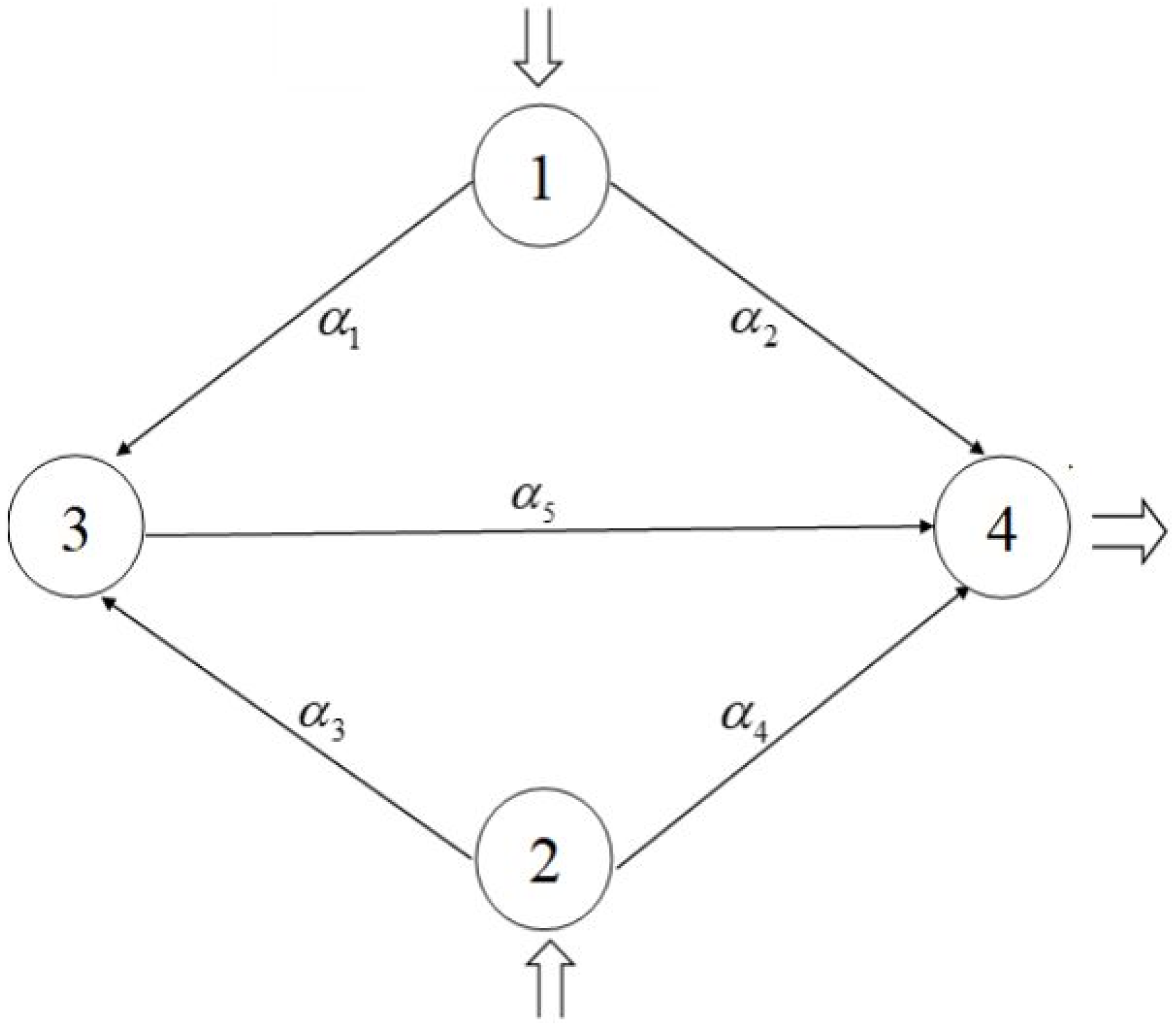
Consider a network problem depicted in Figure 1, where N = { 1 , 2 } , W = { ω } = ( 1 , 2 ) , E = { α 1 , α 2 } , D = d ω = 30 . There are two criteria: travel time and travel cost. The cost functions of arcs and constraints of paths are given as bellow: t 1 , α 1 ( y , ξ ) = y 1 2 + 2 y 1 y 2 + y 2 ξ 1 , t 2 , α 1 ( y , ξ ) = y 1 + y 2 2 ;   t 1 , α 2 ( y , ξ ) = y 1 2 + 10 y 2 y 2 , t 2 , α 2 ( y , ξ ) = 7 y 1 + 6 y 2 2 6 ξ 2 .
l p 1 = 0 , l p 2 = 0 ; u p 1 = 30 , u p 2 = 30 .
Then, we have:
c p 1 ( y , ξ ) = y 1 2 + 2 y 1 y 2 + y 2 ξ 1 y 1 + y 2 2 , c p 2 ( y , ξ ) = y 1 2 + 10 y 2 y 2 7 y 1 + 6 y 2 2 6 ξ 2 .
where ξ 1 [ 0 , 1 ] and ξ 2 [ 0 , 1 ] . Initial feasible flows and a subset of the robust vector equilibrium flows are obtained in 23.82 s . The results are shown in Table 1. However, if we use step calculational method in [22], then it takes 25.68 s and the obtain the same robust vector equilibrium flows with our algorithm.
 Example 3. 
Consider the network problem depicted in Figure 2, where N = { 1 , 2 , 3 , 4 } , W = ( 1 , 4 ) , ( 2 , 4 ) , and there are two O-D pairs, ω 1 , ω 2 . E = { α 1 , α 2 , α 3 , α 4 , α 5 } , p 1 = ( α 1 α 5 ) , p 2 = ( α 2 ) , p 3 = ( α 3 α 5 ) , p 4 = ( α 4 ) , D = { d ω 1 , d ω 2 } = { 55 , 35 } . There are two criteria: travel time and travel cost. Constrains of paths are given as follows:
l p 1 = 0 , l p 2 = 0 , l p 3 = 0 , l p 4 = 0 ;
u p 1 = 55 , u p 2 = 55 , u p 3 = 35 , u p 4 = 35 .
The cost functions of arcs are defined as follows:
t α 1 ( y , ξ ) = y 1 2 + 2 y 2 + y 3 2 + y 4 2 + 1 2 y 1 + y 2 2 + 2 y 3 + y 4 + 3 2 6 ξ 1 , t α 2 ( y , ξ ) = 2 y 1 + 3 y 2 + 5 y 3 + y 4 + 1 + ξ 2 2 y 1 y 2 + y 2 + y 3 2 + y 4 + 1 2 ,
t α 3 ( y , ξ ) = 2 y 1 + y 2 + y 3 2 + y 4 + 3 2 + 3 ξ 3 y 3 2 + 5 y 4 + 1 , t α 4 ( y , ξ ) = 2 y 2 + 3 y 3 y 4 + y 4 2 + 1 y 1 2 + y 2 + y 4 + 1 2 8 ξ 4 , t α 5 ( y , ξ ) = y 1 + y 2 y 3 + y 4 .
Then, we have:
c p 1 ( y , ξ ) = y 1 2 + y 1 + 3 y 2 + y 3 2 + y 4 2 + 1 2 y 1 + y 2 2 + 3 y 3 + 2 y 4 + 1.5 6 ξ 1 , c p 2 ( y , ξ ) = 2 y 1 + 3 y 2 + 5 y 3 + y 4 + 1 + ξ 2 2 y 1 y 2 + y 2 + y 3 2 + y 4 + 0.5
c p 3 ( y , ξ ) = 3 y 1 + 2 y 2 + y 3 2 + y 4 + 1.5 + 3 ξ 3 y 3 2 + y 3 + 6 y 4 + 1 , c p 4 ( y , ξ ) = 2 y 2 + 3 y 3 y 4 + y 4 2 + 1 y 1 2 + y 2 + 8 y 4 + 0.5 8 ξ 4
where ξ i [ 0 , 1 ] , i = 1 , 2 , 3 , 4 . Initial feasible flows and a subset of the robust vector equilibrium flows are obtained in 40.56 s . The results are shown in Table 2. The time cost of Algorithm 1 is 4 % lower than that of the step calculation method in [22].
 Example 4. 
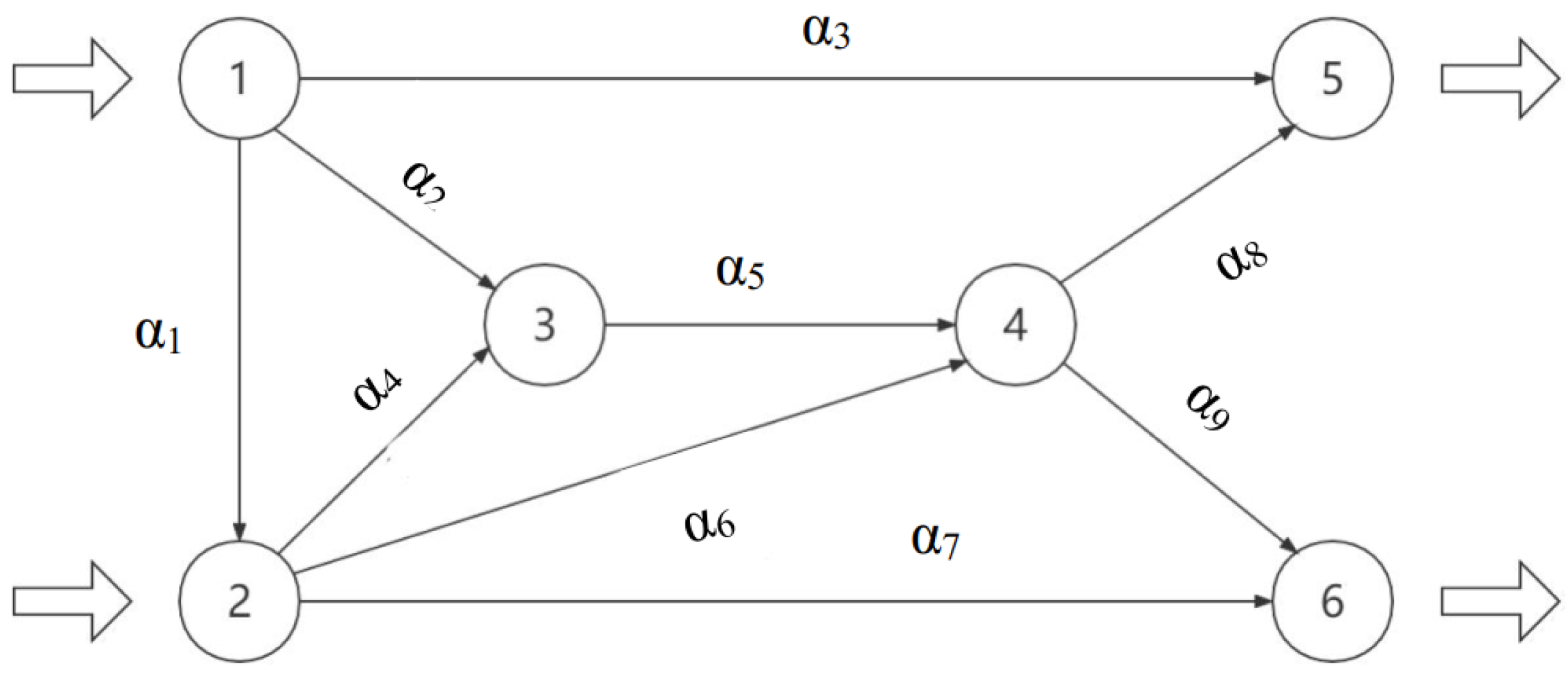
Consider the network problem depicted in Figure 3, where N = { 1 , 2 , 3 , 4 , 5 , 6 } , W = { ω 1 , ω 2 } = ( 1 , 5 ) , ( 2 , 6 ) , E = { α 1 , α 2 , α 3 , α 4 , α 5 , α 6 , α 7 , α 8 , α 9 } , D = { d ω 1 , d ω 2 } , d ω 1 = 25 , d ω 2 = 20 , with two criteria: travel time and travel cost. P ω = { p 1 , p 2 , p 3 , p 4 , p 5 , p 6 , p 7 } , where P ω 1 = { p 1 , p 2 , p 3 , p 4 } , P ω 2 = { p 5 , p 6 , p 7 } , p 1 = ( α 3 ) , p 2 = ( α 2 α 5 α 8 ) , p 3 = ( α 1 α 4 α 5 α 8 ) , p 4 = ( α 1 α 6 α 8 ) , p 5 = ( α 7 ) , p 6 = ( α 6 α 9 ) , and p 7 = ( α 4 α 5 α 9 ) .
The constrains of paths and cost functions are given as follows:
l p 1 = 0 , l p 2 = 0 , l p 3 = 0 , l p 4 = 0 , l p 5 = 0 , l p 6 = 0 , l p 7 = 0 ;
u p 1 = 25 , u p 2 = 25 , u p 3 = 25 , u p 4 = 25 , u p 5 = 20 , u p 6 = 20 , u p 7 = 20 .
t 1 , α 1 ( y , ξ ) = 4 ( y 6 + y 7 ) + 50 2 ξ 3 , t 2 , α 1 ( y , ξ ) = ( y 6 + y 7 ) 2 + 90 2 ξ 3 ;
t 1 , α 2 ( y , ξ ) = 2 y 2 + 20 ξ 2 + 4 ξ 6 , t 2 , α 2 ( y , ξ ) = 3 y 2 2 + 10 ;
t 1 , α 3 ( y , ξ ) = 4 y 1 2 + 100 + ξ 1 , t 2 , α 3 ( y , ξ ) = 2 y 1 2 + 110 + 6 ξ 1 ;
t 1 , α 4 ( y , ξ ) = 2 ( y 4 + y 7 ) + 10 + ξ 2 , t 2 , α 4 ( y , ξ ) = ( y 4 + y 7 ) 2 + 30 ξ 2 + ξ 3 ;
t 1 , α 5 ( y , ξ ) = 2 ( y 3 + y 4 + y 7 ) 2 + 10 ξ 2 , t 2 , α 5 ( y , ξ ) = ( y 3 + y 4 + y 7 ) 2 + 20 + ξ 2 ;
t 1 , α 6 ( y , ξ ) = 5 ( y 4 + y 5 ) 2 + 430 + 2 ξ 3 + ξ 4 , t 2 , α 6 ( y , ξ ) = 2 ( y 4 + y 5 ) + 530 + 2 ξ 3 ξ 4 ;
t 1 , α 7 ( y , ξ ) = 2 y 2 2 + 100 + 5 ξ 5 , t 2 , α 7 ( y , ξ ) = 3 y 5 + 300 ;
t 1 , α 8 ( y , ξ ) = ( y 3 + y 6 + y 7 ) 2 + 20 , t 2 , α 8 ( y , ξ ) = 2 ( y 3 + y 6 + y 7 ) 2 + 10 ;
t 1 , α 9 ( y , ξ ) = ( y 5 + y 6 ) 2 + 30 4 ξ 6 , t 2 , α 9 ( y , ξ ) = 2 ( y 5 + y 6 ) + 10 + 2 ξ 7 ξ 3 ;
where z α i ( i = 1 , 2 , , 9 ) denotes the flow on arc α i . Then we have
c p 1 ( y , ξ ) = 4 y 1 2 + 100 + ξ 1 2 y 1 2 + 110 + 6 ξ 1 , c p 2 ( y , ξ ) = 2 y 2 + 2 ( y 3 + y 4 + y 7 ) 2 + ( y 3 + y 6 + y 7 ) 2 + 50 2 ξ 2 3 y 2 2 + ( y 3 + y 4 + y 7 ) 2 + 2 ( y 3 + y 6 + y 7 ) 2 + 40 + ξ 2
c p 3 ( y , ξ ) = 4 ( y 6 + y 7 ) + 2 ( y 4 + y 7 ) + 2 ( y 3 + y 4 + y 7 ) 2 + ( y 3 + y 6 + y 7 ) 2 + 90 2 ξ 3 ( y 6 + y 7 ) 2 + ( y 4 + y 7 ) 2 + ( y 3 + y 4 + y 7 ) 2 + 2 ( y 3 + y 6 + y 7 ) 2 + 150 ξ 3
c p 4 ( y , ξ ) = 4 ( y 6 + y 7 ) + 5 ( y 4 + y 5 ) 2 + ( y 3 + y 6 + y 7 ) 2 + 500 + ξ 4 ( y 6 + y 7 ) 2 + 2 ( y 4 + y 5 ) + 2 ( y 3 + y 6 + y 7 ) 2 + 630 ξ 4
c p 5 ( y , ξ ) = 2 y 2 2 + 100 + 5 ξ 5 3 y 5 + 300 , c p 6 ( y , ξ ) = 5 ( y 4 + y 5 ) 2 + ( y 5 + y 6 ) 2 + 460 4 ξ 6 2 ( y 4 + y 5 ) + 2 ( y 5 + y 6 ) + 540
c p 7 ( y , ξ ) = 2 ( y 4 + y 7 ) + 2 ( y 3 + y 4 + y 7 ) 2 + ( y 5 + y 6 ) 2 + 50 ( y 4 + y 7 ) 2 + ( y 3 + y 4 + y 7 ) 2 + 2 ( y 5 + y 6 ) 2 + 60 + 2 ξ 7
where ξ i [ 0 , 1 ] , i = 1 , 2 , 3 , 4 , 5 , 6 , 7 . Initial feasible flows and a subset of the robust vector equilibrium flows are obtained in 538.47  s. The results are shown in Table 3. The algorithm proposed in [22] obtains the same robust vector equilibrium flows, but its time cost is 548.32 s.

4. Smoothing Method for the Robust Vector Equilibrium with the Worst Case

It is worth noting that the algorithm in [21] needs to solve a non-smoothing optimization problem. This results in its computational inefficiency. This prompts us to continuously investigate algorithm for solving robust equilibrium flows. In this section, we propose a smoothing method to calculate a subset of the robust vector equilibrium with respect to the worst case. The algorithm is denoted Algorithm 3. To generalize a subset of the robust vector equilibrium flows with respect to the worst case, we use a two-step strategy. The first step is to construct an equivalent optimization problem with the help of a variant version of ReLU activation function for finding the robust weak vector equilibrium flows with respect to the worst case. The second step is to judge whether or not the robust weak vector equilibrium flows with respect to the worst case are equal to the robust vector equilibrium flows with respect to the worst case by an equivalent optimization problem using the vector version of heaviside step function.
Algorithm 3: Robust vector equilibrium algorithm (denoted Algorithm 3).
        1
Choose a positive integer q and a tolerance level ϵ 0 .
        2
Enter l = ( l p k ) p k P and u = ( u p k ) P k P . Set δ j = d ω j / ( q | P ω j | ) , j = 1 , , l ˜ .
        3
Choose ( k 1 , , k n ) N n satisfying
i I j k i = q | P ω j | , and l p i k i δ j u p i , i I j , j = 1 , , l ˜ .
        4
Store y = ( y p 1 , , y p n ) in S 0 where
y p i = k i δ j , i I j , j = 1 , , l ˜
and return to Step 3 for other vectors ( k 1 , , k n ) unless no one left.
        5
Choose a feasible flow y 0 from S 0 to start. Set k = 0 , S 0 = S 0 { y 0 } and W E = .
        6
For every i , j { 1 , , n } , solve
minimize ϕ ( y ) subject to y Ω y p i y p i 0 δ ω ( i ) , i = 1 , , n .
If ϕ ( y ) ϵ , store y in W E and return to Step 5 until no element of S 0 left.
        7
Choose a feasible flow y W E , W E = W E { y } .
        8
Compute
φ ( y ) = ω W p k , p j P ω ( y p k l p k ) ( u p j y p j ) ( C p k ( y ) C p j ( y ) ) H + [ C p k ( y ) C p j ( y ) ]
        9
If φ ( y ) ϵ , store y in E and return to Step 7 until no element of W E left.
Define a function r : R R and give its vector version function R : R n R m as follows:
r ( a ) = m a x { 0 , a } 2 .
R ( x ) = ( i = 1 n r ( x i ) ) e ,
In addition, the heaviside step function h + : R R and its vector version function H + : R n R m are also given below:
h + ( a ) = 1 , if a 0 , 0 , o t h e r w i s e .
H + ( x ) = ( i = 1 n h + ( x i ) ) e , x R m .

4.1. Description of the Algorithm

In this subsection, we construct an optimization problem whose solution is equivalent to a robust weak vector equilibrium flow with respect to the worst case. For y Ω , we define:
ϕ ( y ) : = ω W p k , p j P ω ( y p k l p k ) ( u p j y p j ) ( C p k ( y ) C p j ( y ) ) R [ C p k ( y ) C p j ( y ) ] .
 Proposition 2. 
Let y ¯ be a feasible flow. The following statements are equivalent.
 (i) 
y ¯ is a robust weak vector equilibrium with respect to the worst case;
 (ii) 
y ¯ is an optimal solution of the problem, denoted:
min ϕ ( y ¯ ) s . t . y Ω .
and the optimal value ϕ ( y ¯ ) is equal to zero.
 Proof. 
We first prove the implication ( i ) ( i i ) . It is not hard to see ϕ ( y ) 0 for every y Ω . Thus, if y ¯ is a robust weak vector equilibrium with respect to the worst case, in order to deduce (ii), it suffices to prove ϕ ( y ¯ ) = 0 . In addition, for every p k p ω , ω W , consider the term:
Q p = ω W p k , p j P ω ( y p k l p k ) ( u p j y p j ) ( C p k ( y ) C p j ( y ) ) R [ C p k ( y ) C p j ( y ) ] .
If C p k ( y ¯ ) C p j ( y ¯ ) 0 R m , for some p j P ω , then by Definition 3, either y ¯ p k = l p k or y ¯ p j = u p j ; if C p k ( y ¯ ) C p j ( y ¯ ) = 0 R m , for some p j P ω , we also get Q p = 0 ; if C p k ( y ¯ ) C p j ( y ¯ ) 0 R m , then R [ C p k ( y ) C p j ( y ) ] = 0 R m , and thus, Q p = 0 . As a result, one has ϕ ( y ¯ ) = 0 .
Conversely, assume that y ¯ is an optimal solution of Problem (3) and ϕ ( y ¯ ) = 0 . Then, we have Q p = 0 for all p P . If there exists some p k , p j p ω , ω W such that C p k ( y ¯ ) C p j ( y ¯ ) 0 R m , then ( C p k ( y ) C p j ( y ) ) R [ C p k ( y ) C p j ( y ) 0 R m , and thus, either y ¯ p k = l p k or y ¯ p j = u p j by Q p = 0 . Consequently, we deduce that y ¯ is a robust weak vector equilibrium with respect to the worst case. □
For y Ω , we define
φ ( y ) = ω W p k , p j P ω ( y p k l p k ) ( u p j y p j ) ( C p k ( y ) C p j ( y ) ) H + [ C p k ( y ) C p j ( y ) ] .
Then, by using a similar method of proof, we may establish the following result for the robust vector equilibrium with respect to the worst case.
 Proposition 3. 
Let y ¯ be a feasible flow. The following statements are equivalent.
 (i) 
y ¯ is a robust vector equilibrium with respect to the worst case.
 (ii) 
y ¯ is an optimal solution of the problem, denoted as follows:
min φ ( y ) s . t . y Ω .
and the optimal value φ ( y ¯ ) is equal to zero.
Algorithm 3 is mainly based on ideas of Propositions 2 and 3. Steps  1–4 create a subset of feasible flows with the initial conditions, denoted as S 0 , with which Steps  4–6 will start. Steps  5–6 are aimed at solving Problem (3) given in Proposition 2 by using first-order optimization methods, and then a subset of the robust weak vector equilibrium flows with respect to the worst case is gained. Steps  7–9 focus on solving Problem (4) given in Proposition 3, and then a subset of the robust vector equilibrium flows with respect to the worst case is generated.
Assume that W consists of l ˜ elements ω 1 , , ω l ˜ in the network and for each pair ω i . Let I j = i 1 , , n : p i P w j . Denote W E by the subset of the robust weak vector equilibrium flows with respect to the worst case and E by the subset of the robust vector equilibrium flows with respect to worst case.

4.2. Comparison with Other Methods

In this subsection, we will give two numerical examples to show the comparison with that of [21]. In these numerical examples, both Algorithm 3 and the algorithm proposed in [21] start from the same set of initial points. To make a fair comparison, all test problems are run five times to reduce the impact of randomness.
 Example 5. 
Consider the network problem depicted in Figure 4, where N = { 1 , 2 , 3 , 4 , 5 } , W = { ω 1 , ω 2 } = ( 1 , 4 ) , ( 1 , 5 ) , E = { α 1 , α 2 , α 3 , α 4 , α 5 , α 6 , α 7 , α 8 , α 9 } , D = { d ω 1 , d ω 2 } , d ω 1 = 25 , d ω 2 = 20 , with two criteria: travel time and travel cost, P ω = { p 1 , p 2 , p 3 , p 4 , p 5 , p 6 , p 7 } , where P ω 1 = { p 1 , p 2 , p 3 , p 4 } , P ω 2 = { p 5 , p 6 , p 7 } .
Assume that:
l p 1 = l p 2 = l p 3 = l p 4 = l p 5 = l p 6 = l p 7 = l p 8 = 0 ;
u p 1 = 100 , u p 2 = 100 , u p 3 = 100 , u p 4 = 200 , u p 5 = 100 , u p 6 = 120 , u p 7 = 150 , u p 8 = 100 ;
t 1 , α 1 ( y , ξ ) = y 1 2 + y 2 2 + y 3 3 + ξ 1 , t 2 , α 1 ( y , ξ ) = 2 y 1 + 5 y 2 + 3 y 3 + y 4 2 ξ 1 ;
t 1 , α 2 ( y , ξ ) = 8 y 1 y 2 + y 2 2 + y 7 + y 8 + 4 ξ 2 , t 2 , α 2 ( y , ξ ) = y 2 + 10 y 3 + 2 y 7 + y 8 + 2 ξ 2 ;
t 1 , α 3 ( y , ξ ) = y 1 + y 2 2 + y 3 3 + y 5 + y 6 3 ξ 3 , t 2 , α 3 ( y , ξ ) = 10 y 3 3 + 2 y 5 + ξ 3 ;
t 1 , α 4 ( y , ξ ) = y 1 + y 2 + y 4 3 + y 5 2 + y 8 3 + ξ 4 , t 2 , α 4 ( y , ξ ) = y 1 + 2 y 4 + y 6 y 5 + 15 y 8 ;
t 1 , α 5 ( y , ξ ) = y 1 + y 3 + y 4 3 + y 5 2 + y 6 2 , t 2 , α 5 ( y , ξ ) = y 1 + 5 y 3 + 5 y 5 + 3 y 6 + 12 y 7 + 4 ξ 5 ;
t 1 , α 6 ( y , ξ ) = y 3 + y 4 + y 5 + y 6 3 3 ξ 6 , t 2 , α 6 ( y , ξ ) = 3 y 3 + 10 y 5 + y 6 + 2 y 8 2 ξ 6 ;
t 1 , α 7 ( y , ξ ) = y 2 + 8 y 4 2 + y 5 + y 7 3 + 2 ξ 7 , t 2 , α 7 ( y , ξ ) = y 1 + y 2 + 5 y 4 + 3 y 7 ;
t 1 , α 8 ( y , ξ ) = y 1 + y 3 + 8 y 6 y 7 + y 8 2 + ξ 8 , t 2 , α 8 ( y , ξ ) = y 1 + y 3 + 10 y 5 3 + y 8 ξ 8 ,
where ξ i [ 0 , 1 ] , i = 1 , 2 , 3 , 4 , 5 , 6 , 7 , 8 . Then, we have
C p 1 ( y ) = y 1 2 + y 2 2 + y 3 3 + 1 2 y 1 + 5 y 2 + 3 y 3 + y 4 , C p 2 ( y ) = 8 y 1 y 2 + y 2 2 + y 7 + y 8 + 4 y 2 + 10 y 3 + 2 y 7 + y 8 + 2
C p 3 ( y ) = y 1 + y 2 2 + y 3 3 + y 5 + y 6 10 y 3 3 + 2 y 5 + 1 , C p 4 ( y ) = y 1 + y 2 + y 4 3 + y 5 2 + y 8 3 + 1 y 1 + 2 y 4 + y 6 y 5 + 15 y 8
C p 5 ( y ) = y 1 + y 3 + y 4 3 + y 5 2 + y 6 2 y 1 + 5 y 3 + 5 y 5 + 3 y 6 + 12 y 7 + 4 , C p 6 ( y ) = y 3 + y 4 + y 5 + y 6 3 3 y 3 + 10 y 5 + y 6 + 2 y 8
C p 7 ( y ) = y 2 + 8 y 4 2 + y 5 + y 7 3 + 2 y 1 + y 2 + 5 y 4 + 3 y 7 , C p 8 ( y ) = y 1 + y 3 + 8 y 6 y 7 + y 8 2 + 1 y 1 + y 3 + 10 y 5 3 + y 8
Choosing q = 2 , we have 32 feasible flows and 2 robust (weak) vector equilibrium flows with respect to the worst case, which are obtained in 0.18 s . Robust (weak) vector equilibrium flows with respect to the worst case are shown in Table 4. However, using the algorithm proposed in [21], it will take 13.826 s to obtain five robust vector equilibrium flows with respect to the worst case, which are shown in Table 5.
 Example 6. 
Consider the network problem depicted in Figure 5, where N = { 1 , 2 , 3 , 4 , 5 } , W = { ω 1 , ω 2 } = ( 1 , 4 ) , ( 1 , 5 ) , E = { α 1 , α 2 , α 3 , α 4 , α 5 , α 6 , α 7 , α 8 , α 9 } , D = { d ω 1 , d ω 2 } with d ω 1 = 25 , d ω 2 = 20 , with two criteria: travel time and travel cost, P ω = { p 1 , p 2 , p 3 , p 4 , p 5 , p 6 , p 7 } , where P ω 1 = { p 1 , p 2 , p 3 , p 4 } , P ω 2 = { p 5 , p 6 , p 7 } . p 1 = ( α 4 ) , p 2 = ( α 2 α 8 ) , p 3 = ( α 2 α 6 α 3 ) , p 4 = ( α 1 α 3 ) , p 5 = ( α 5 ) , p 6 = ( α 2 α 9 ) , p 7 = ( α 1 α 7 ) . Let:
l 1 = 0 , l 2 = 0 , l 3 = 0 , l 4 = 0 , l 5 = 0 , l 6 = 0 , l 7 = 0 ;
u 1 = 15 , u 2 = 20 , u 3 = 15 , u 4 = 10 , u 5 = 15 , u 6 = 10 , u 7 = 15 .
Now, we give the cost function of arcs as follows:
t α 1 ( y , ξ ) = 4 ( y 6 + y 7 ) + 2 ( y 3 + y 4 + y 7 ) 2 + 300 2 ξ 1 ( y 6 + y 7 ) 2 + ( y 3 + y 4 + y 7 ) 2 + 330 ξ 1 , t α 2 ( y , ξ ) = 2 ( y 3 + y 4 + y 7 ) 2 + 50 + ξ 2 ( y 3 + y 4 + y 7 ) 2
t α 3 ( y , ξ ) = 2 ( y 3 + y 7 ) + 2 ( y 4 + y 7 ) 2 + 300 + 2 ξ 1 + ξ 6 ( y 3 + y 7 ) 2 + 2 ( y 4 + y 7 ) + 100 + ξ 1 ξ 3 , t α 4 ( y , ξ ) = 4 y 1 2 + 100 + ξ 4 2 y 1 2 + 110 + 6 ξ 4
t α 5 ( y , ξ ) = 2 y 2 2 + 100 + 5 ξ 5 3 y 2 + y 5 + 300 , t α 6 ( y , ξ ) = ( y 3 + y 6 + y 7 ) 2 260 ξ 6 ξ 2 2 ( y 3 + y 6 + y 7 ) 2 + 50 ξ 1
t α 7 ( y , ξ ) = 2 ( y 3 + y 7 ) + 2 ( y 4 + y 7 ) 2 150 + 3 ξ 1 ξ 7 ( y 3 + y 7 ) 2 + ( y 4 + y 7 ) 2 310 + ξ 1 , t α 8 ( y , ξ ) = 2 y 2 + ( y 3 + y 6 + y 7 ) 2 ξ 2 3 y 2 2 + 2 ( y 3 + y 6 + y 7 ) 2 + 40 ξ 8
t α 9 ( y , ξ ) = 5 ( y 5 + y 6 ) 2 + 410 + ξ 2 2 ( y 5 + y 6 ) 2 + 540 ξ 9
where ξ i [ 0 , 1 ] , i = 1 , 2 , 3 , 4 , 5 , 6 , 7 , 8 , 9 . Then, we have:
C p 1 ( y ) = 4 y 1 2 + 101 2 y 1 2 + 116 , C p 2 ( y ) = 2 y 2 + 2 ( y 3 + y 4 + y 7 ) 2 + ( y 3 + y 6 + y 7 ) 2 + 50 3 y 2 2 + ( y 3 + y 4 + y 7 ) 2 + 2 ( y 3 + y 6 + y 7 ) 2 + 41 ,
C p 3 ( y ) = 4 ( y 3 + y 7 ) + 2 ( y 4 + y 7 ) 2 + 2 ( y 3 + y 4 + y 7 ) 2 + ( y 3 + y 6 + y 7 ) 2 + 90 ( y 3 + y 7 ) 2 + 2 ( y 4 + y 7 ) + ( y 3 + y 4 + y 7 ) 2 + 2 ( y 3 + y 6 + y 7 ) 2 + 150 ,
C p 4 ( y ) = 4 ( y 3 + y 7 ) + 2 ( y 4 + y 7 ) 2 + 4 ( y 6 + y 7 ) + 2 ( y 3 + y 4 + y 7 ) 2 + 601 ( y 3 + y 7 ) 2 + 2 ( y 4 + y 7 ) + ( y 6 + y 7 ) 2 + ( y 3 + y 4 + y 7 ) 2 + 430 ,
C p 5 ( y ) = 2 y 2 2 + 105 3 y 2 + y 5 + 300 , C p 6 ( y ) = 5 ( y 5 + y 6 ) 2 + 2 ( y 3 + y 4 + y 7 ) 2 + 460 2 ( y 5 + y 6 ) + ( y 3 + y 4 + y 7 ) 2 + 540 ,
C p 7 ( y ) = 4 ( y 6 + y 7 ) + 2 ( y 4 + y 7 ) 2 + 2 ( y 3 + y 4 + y 7 ) 2 + 2 ( y 3 + y 7 ) + 152 ( y 6 + y 7 ) 2 + ( y 4 + y 7 ) 2 + ( y 3 + y 4 + y 7 ) 2 + ( y 3 + y 7 ) 2 + 20 .
Choosing q = 1 , 80 feasible flows are created and a subset of robust vector equilibrium flows with respect to the worst case (displayed in Table 6) are obtained. This takes about 0.62 s . However, using the algorithm presented in [21], it spends 579 s to obtain a subset of robust vector equilibrium flows with respect to the worst case, which are shown in Table 7.

5. Conclusions

In this paper, we mainly consider a robust multi-criteria traffic network equilibrium problem with path capacity constraints. Firstly, the robust vector equilibrium principle and the robust vector equilibrium principle with respect to the worst case are given. We pay attention to constructing an equivalent min–max optimization problem for the robust vector equilibrium, in which the solution is equivalent to a robust vector equilibrium. Then, a direct search algorithm is proposed for solving the corresponding min–max optimization problem. The step size in the algorithm requires neither gradient information nor redundant parameters. What is more, we select different step sizes for different variables and extend the search directions. The results of three numerical experiments show that it takes less time than the method in [22] to find the robust vector equilibrium flows.
To generate a subset of the robust vector equilibrium with respect to the worst case, we employ a two-step strategy. The first step is to construct a smoothing optimization problem based on a variant version of the ReLU activation function to compute the robust weak vector equilibrium flows with respect to the worst case. The second step is to judge whether or not the robust weak vector equilibrium flows with respect to the worst case are equal to the robust vector equilibrium flows with respect to the worst case. Compared with the algorithm in [21], the results of two numerical experiments show that our algorithm can greatly reduce the computational cost.
Recently, robust vector optimization based on set orders is widely used in the uncertain optimization environment [23,24]. It is noteworthy that the robust vector equilibrium principles considered in this paper are all based on vector order. In addition, our method can only be applied to small-scale traffic networks. Therefore, an interesting topic for future research is to investigate large-scale, multi-criteria traffic networks based on set orders.

Author Contributions

Conceptualization, X.-X.M. and Y.-D.X.; Writing—original draft preparation, X.-X.M. and Y.-D.X.; Writing—review and editing, X.-X.M. and Y.-D.X. All authors have read and agreed to the published version of the manuscript.

Funding

This research was supported by the National Natural Science Foundation of China (Grant number: 11801051) and the Natural Science Foundation of Chongqing (Grant number: cstc2019jcyj-msxmX0075).

Data Availability Statement

The data that support the findings of this study are available from the corresponding author upon reasonable request.

Conflicts of Interest

The authors declare no conflict of interest.

References

  1. Wardrop, J. Some theoretical aspects of road traffic research. Proc. Inst. Civil Eng. Part II 1952, 1, 325–362. [Google Scholar] [CrossRef]
  2. Athanasenas, A. Traffic simulation model for rural road network management. Trans. Res. Part E 1997, 33, 233–243. [Google Scholar] [CrossRef]
  3. Nagurney, A. On the relationship between supply chain and transportation network equilibria: A super network equivalence with computations. Trans. Res. Part E 2006, 42, 293–316. [Google Scholar] [CrossRef] [Green Version]
  4. Ji, X.F.; Chu, Y.Y. A target-oriented bi-attribute user equilibrium model with travelers perception errors on the tolled traffic network. Trans. Res. Part E 2020, 144, 102–150. [Google Scholar] [CrossRef]
  5. Xu, Z.T.; Chen, Z.B.; Yin, Y.F.; Ye, J.P. Equilibrium analysis of urban traffic networks with ride-sourcing services. Trans. Sci. 2021, 55, 1227–1458. [Google Scholar] [CrossRef]
  6. Wang, J.; Du, M.Q.; Lu, L.L.; He, X.Z. Maximizing network throughput under stochastic user equilibrium with elastic demand. Netw. Spat. Econ. 2018, 18, 115–143. [Google Scholar] [CrossRef]
  7. Ma, J.; Meng, Q.; Cheng, L.; Liu, Z.Y. General stochastic ridesharing user equilibrium problem with elastic demand. Trans. Res. Part B 2022, 162, 162–194. [Google Scholar] [CrossRef]
  8. Chen, G.Y.; Yen, N.D. On the Variational Inequality Model for Network Equilibrium; Internal Report 3; Department of Mathematics, University of Pisa: Pisa, Italy, 1993; Volume 196. [Google Scholar]
  9. Yang, X.Q.; Goh, C.J. On vector variational inequalities: Application to vector equilibria. J. Optim. Theory Appl. 1997, 95, 431–443. [Google Scholar] [CrossRef]
  10. Li, S.J.; Teo, K.L.; Yang, X.Q. A remark on a standard and linear vector network equilibrium problem with capacity constraints. Eur. J. Oper. Res. 2008, 184, 13–23. [Google Scholar] [CrossRef] [Green Version]
  11. Luc, D.T.; Rocca, M.; Papalia, M. Equilibrium in a vector supply demand network with capacity. Appl. Anal. 2011, 90, 1029–1045. [Google Scholar] [CrossRef]
  12. Raith, A.; Ehrgott, A. On vector equilibria, vector optimization and vector variational inequalities. J. Multi-Crit. Decis. Anal. 2011, 18, 39–54. [Google Scholar] [CrossRef]
  13. Phuong, T.T.T.; Luc, D.T. Equilibrium in multi-criteria supply and demand networks with capacity constraints. Math. Methods Oper. Res. 2015, 81, 83–107. [Google Scholar]
  14. Luc, D.T.; Phuong, T.T.T. Equilibrium in multi-criteria transportation networks. J. Optim. Theory Appl. 2016, 169, 116–147. [Google Scholar] [CrossRef]
  15. Phuong, T.T.T. Smoothing method in multi-criteria transportation network equilibrium problem. Optimization 2019, 68, 1577–1598. [Google Scholar] [CrossRef]
  16. Daniele, P.; Giuffré, S. Random variational inequalities and the random traffic equilibrium problem. J. Optim. Theory Appl. 2015, 167, 363–381. [Google Scholar] [CrossRef]
  17. Dragicevic, A.; Gurtoo, A. Stochastic Control of Ecological Networks. J. Math. Biol. 2022, 85, 7. [Google Scholar] [CrossRef]
  18. Ehrgott, M.; Wang, J.Y.T.; Watling, D.P. On multi-objective stochastic user equilibrium. Trans. Res. Part B 2015, 81, 704–717. [Google Scholar] [CrossRef] [Green Version]
  19. Cao, J.D.; Li, R.X.; Huang, W.; Guo, J.H.; Wei, Y. Traffic network equilibrium problems with demands uncertainty and capacity constraints of arcs by scalarization approaches. Sci. China Technol. Sci. 2018, 61, 1642–1653. [Google Scholar] [CrossRef]
  20. Wei, H.Z.; Chen, C.R.; Wu, B.W. Vector network equilibrium problems with uncertain demands and capacity constraints of arcs. Optim. Lett. 2021, 15, 1113–1131. [Google Scholar] [CrossRef]
  21. Minh, N.B.; Phuong, T.T.T. Robust equilibrium in transportation networks. Acta Math. Vietnam. 2020, 45, 635–650. [Google Scholar] [CrossRef]
  22. Dzahini, K.J. Expected complexity analysis of stochastic direct-search. Comput. Optim. Appl. 2022, 81, 1–22. [Google Scholar] [CrossRef]
  23. Bouza, G.; Quintana, E.; Tammer, C. A steepest descent method for set optimization problems with set-valued mappings of finite cardinality. J. Optim. Theory Appl. 2021, 190, 711–743. [Google Scholar] [CrossRef]
  24. Eichfelder, G.; Quintana, E.; Rocktäschel, S. A vectorization scheme for nonconvex set optimization problems. SIAM J. Optim. 2022, 32, 1184–1209. [Google Scholar] [CrossRef]
Figure 1. Network topology for Example 2.
Axioms 12 00662 g001
Figure 2. Network topology for Example 3.
Axioms 12 00662 g002
Figure 3. Network topology for Example 4.
Axioms 12 00662 g003
Figure 4. Network topology for Example 5.
Axioms 12 00662 g004
Figure 5. Network topology for Example 6.
Axioms 12 00662 g005
Table 1. Computational results of Algorithm 1.
Initial Feasible FlowsRobust Vector Equilibrium Flows
( 0.00 , 30.00 ) ( 3.75 , 26.25 ) ( 25.00 , 5.00 ) ( 25.75 , 4.25 )
( 11.25 , 18.75 ) ( 11.25 , 18.75 ) ( 25.50 , 4.50 ) ( 25.25 , 4.75 )
( 15.00 , 15.00 ) ( 18.75 , 11.25 ) ( 25.00 , 5.00 ) ( 25.75 , 4.25 )
( 22.50 , 7.50 ) ( 26.25 , 3.75 ) ( 25.50 , 4.50 ) ( 26.25 , 3.75 )
( 30.00 , 0.00 ) ( 30.00 , 0.00 )
Table 2. Computational results of Algorithm 1.
Initial Feasible FlowsRobust Vector Equilibrium Flows
(0.00, 55.00, 0.00, 35.00)(27.00, 28.00, 27.00, 8.00)
(5.00, 50.00, 5.00, 30.00)(27.00, 28.00, 27.00, 8.00)
(10.00, 45.00, 10.00, 25.00)(27.00, 28.00, 27.00, 8.00)
(15.00, 40.00, 15.00, 20.00)(27.00, 28.00, 27.00, 8.00)
(20.00, 35.00, 20.00, 15.00)(27.00, 28.00, 27.00, 8.00)
(25.00, 30.00, 25.00, 10.00)(29.00, 26.00, 29.00, 6.00)
(30.00, 25.00, 30.00, 5.00)(29.00, 26.00, 29.00, 6.00)
(35.00, 20.00, 35.00, 0.00) 
Table 3. Computational results of Algorithm 1.
Initial Feasible FlowsRobust Vector Equilibrium Flows
( 0 , 0 , 0 , 25 , 0 , 0 , 20 )   ( 0 , 0 , 25 , 0 , 0 , 0 , 20 ) ( 9 , 7 , 9 , 0 , 19 , 0 , 1 )   ( 12 , 13 , 0 , 0 , 8 , 0 , 12 )
( 0 , 25 , 0 , 0 , 0 , 0 , 20 )   ( 25 , 0 , 0 , 0 , 0 , 0 , 20 ) ( 15 , 10 , 0 , 0 , 9 , 0 , 11 )   ( 15 , 10 , 0 , 0 , 9 , 0 , 11 )
( 0 , 0 , 0 , 25 , 0 , 20 , 0 )   ( 0 , 0 , 25 , 0 , 0 , 20 , 0 ) ( 12 , 8 , 5 , 0 , 15 , 0 , 5 )   ( 15 , 10 , 0 , 0 , 9 , 0 , 11 )
( 0 , 25 , 0 , 0 , 0 , 20 , 0 )   ( 25 , 0 , 0 , 0 , 0 , 20 , 0 ) ( 9 , 7 , 9 , 0 , 19 , 0 , 1 )   ( 12 , 13 , 0 , 0 , 8 , 0 , 12 )
( 0 , 0 , 0 , 25 , 20 , 0 , 0 )   ( 0 , 0 , 25 , 0 , 20 , 0 , 0 ) ( 11 , 7 , 7 , 0 , 18 , 0 , 2 )
( 0 , 25 , 0 , 0 , 20 , 0 , 0 )   ( 25 , 0 , 0 , 0 , 20 , 0 , 0 )  
Table 4. Computational results of Algorithm 3.
Robust Weak Vector Equilibrium Flows (Worst Case)Robust Vector Equilibrium Flows (Worst Case)
( 100 , 100 , 100 , 145.125 , 0 , 120 , 134.875 , 100 ) ( 100 , 100 , 100 , 145.125 , 0 , 120 , 134.875 , 100 )
( 100 , 100 , 100 , 150 , 0 , 120 , 130 , 100 ) ( 100 , 100 , 100 , 150 , 0 , 120 , 130 , 100 )
Table 5. Computational results of algorithm in [21].
Robust Vector Equilibrium Flows (Worst Case)
( 100 , 100 , 100 , 30 , 100 , 120 , 150 , 100 )
( 100 , 100 , 100 , 50 , 100 , 120 , 130 , 100 )
( 100 , 100 , 100 , 100 , 100 , 120 , 80 , 100 )
( 100 , 100 , 100 , 150 , 100 , 120 , 30 , 100 )
( 100 , 100 , 100 , 200 , 100 , 100 , 100 , 0 )
Table 6. Computational results of Algorithm 3.
Robust Weak Vector Equilibrium Flows (Worst Case)Robust Vector Equilibrium Flows (Worst Case)
( 11.88 , 11.29 , 1.83 , 0 , 13.23 , 0 , 6.77 ) ( 11.88 , 11.29 , 1.83 , 0 , 13.23 , 0 , 6.77 )
( 10.56 , 12.5 , 1.94 , 0 , 13.33 , 0 , 6.67 ) ( 10.56 , 12.5 , 1.94 , 0 , 13.33 , 0 , 6.67 )
( 10.04 , 14.92 , 0.04 , 0 , 11.89 , 0 , 8.11 ) ( 10.04 , 14.92 , 0.04 , 0 , 11.89 , 0 , 8.11 )
( 11.03 , 12.4 , 1.57 , 0 , 13.33 , 0 , 6.67 ) ( 11.03 , 12.4 , 1.57 , 0 , 13.33 , 0 , 6.67 )
( 11.42 , 13.58 , 0 , 0 , 11.93 , 0 , 8.07 ) ( 11.42 , 13.58 , 0 , 0 , 11.93 , 0 , 8.07 )
( 10.45 , 12.5 , 2.05 , 0 , 13.33 , 0 , 6.67 ) ( 10.45 , 12.5 , 2.05 , 0 , 13.33 , 0 , 6.67 )
( 11.12 , 10 , 3.88 , 0 , 15 , 0 , 5 ) ( 11.12 , 10 , 3.88 , 0 , 15 , 0 , 5 )
Table 7. Computational results of algorithm in [21].
Robust Vector Equilibrium Flows (Worst Case)
( 10.94 , 12.5 , 1.56 , 0 , 12.29 , 0 , 7.71 )
( 10.94 , 13.28 , 0.78 , 0 , 12.29 , 0 , 7.71 )
( 12.66 , 10.78 , 1.56 , 0 , 12.29 , 0 , 7.71 )
( 10.94 , 12.5 , 1.56 , 0 , 12.5 , 0 , 7.5 )
Disclaimer/Publisher’s Note: The statements, opinions and data contained in all publications are solely those of the individual author(s) and contributor(s) and not of MDPI and/or the editor(s). MDPI and/or the editor(s) disclaim responsibility for any injury to people or property resulting from any ideas, methods, instructions or products referred to in the content.