Article

New Wave Solutions for the Two-Mode Caudrey–Dodd–Gibbon Equation

by
Rodica Cimpoiasu
1,† and
Radu Constantinescu
2,*,†
1
Applied Life Sciences and Biotechnologies Research Center, University of Craiova, 13 A. I. Cuza Street, 200585 Craiova, Romania
2
Department of Physics, University of Craiova, 13 A. I. Cuza Street, 200585 Craiova, Romania
*
Author to whom correspondence should be addressed.
These authors contributed equally to this work.
Axioms 2023, 12(7), 619; https://doi.org/10.3390/axioms12070619
Submission received: 17 May 2023 / Revised: 14 June 2023 / Accepted: 20 June 2023 / Published: 21 June 2023
(This article belongs to the Special Issue Special Topics in Differential Equations with Applications)

Abstract

:
In this paper, we present new dynamical properties of the two-mode Caudrey–Dodd–Gibbon (TMCDG) equation. This equation describes the propagation of dual waves in the same direction with different phase velocities, dispersion parameters, and nonlinearity. This study takes a full advantage of the Kudryashov method and of the exponential expansion method. For the first time, dual-wave solutions are obtained for arbitrary values of the nonlinearity and dispersive factors. Graphs of the novel solutions are included in order to show the waves’ propagation, as well as the influence of the involved parameters.

1. Introduction

Two-mode nonlinear partial differential equations (NPDEs) represent extensions of the usual NPDEs. Both types of NPDEs, standard and two-mode, play a considerable role in explaining nonlinear phenomena appearing in nature [1]. Two-mode equations describe the interaction of solitons in gravitation, or the slow–fast propagation of waves in hydrodynamics. They can also model dynamical phenomena in variable magnetic fields appearing in plasma physics.
Standard evolutionary NPDEs involve a first-order partial derivative with respect to time, and describe the unidirectional motion of a single wave. Dual/two-mode equations are NPDEs of a second order in time, and govern the evolution of two-wave modes, propagating in the same direction and with the same dispersion relation, while the phase velocity and the linear and nonlinear parameters are different. The current investigations of the two-mode waves mainly use the method proposed by Korsunsky [2]. It shows that to derive the two-mode PDEs, it is necessary to collect, as two distinct components, the nonlinear terms N ( u , u x u , ) and the linear terms L ( u q x , q 2 ) , other than u t . in the last period of time, many authors considered topics related to two-mode PDEs [3,4,5,6]. The dynamics of the two-mode KdV equation associated with the standard-mode third -order KdV equation was studied by various analytical methods, including reductive perturbation [7], the Hamiltonian system [8], or Bell polynomials [9]. In [10], it was shown that the two modes are solitons that continue to propagate separately, without shape and velocity changes, and with the only effect of their collision consisting of some phase shifts. Rather similar methods to what we will apply in our paper, namely the Kudryashov and exponential expansion methods, were used in [11] for the two-mode Sawada–Kotera equation. Bright, dark, periodic, and singular-periodic dual-wave solutions were constructed using a slight different auxiliary equation, as we will consider here. In [12] a dual-mode version of the nonlinear Schrödinger equation was studied, and its solution was expressed as a finite series of tanh-sech functions. More exactly, dual-mode dark and singular soliton solutions were obtained. The tanh expansion method and Kudryashov technique were used in [13] with the dual-mode Kadomtsev–Petviashvili equation to find the necessary constraint conditions that guarantee the existence of soliton solutions. Multiple kink solutions were pointed out in [14] for the two-mode Sharma–Tasso–Olver equation, as well as for the two-mode fourth-order Burgers equation by using the Cole–Hopf transformation combined with the simplified Hirota method. Three different techniques, including the Kudryashov expansion method that will be used here, were applied in [15] in order to study the dynamic behaviors for a dual-mode generalized Hirota–Satsuma coupled KdV system.
The contributions of this work are twofold. First, we find explicit dual-wave solutions for the dual/two-mode Caudrey–Dodd–Gibbon (TMCDG) equation for arbitrary nonlinearity and dispersion parameters, α and β . Previously, only the case α = β = ± 1 was considered in [16], using the Hirota method. The same method was applied in [17] on a more general form of TMCDG. Second, we study the influence of the mentioned parameters, as well as of s , which stands for phase velocity, on the wave propagations, showing how the dual-wave propagation depends on them.
The paper is organized as follows: After the Introduction, in Section 2, an overview on the general form of the TMCDG equation is provided. In Section 3 we present basic facts on the Kudryashov method [18,19] and the exponential expansion method [20]. The findings of our investigation, where the previous methods were applied to the TMCDG equation, are pointed out in Section 4. The analytical results were obtained using the Maple program. Some graphical representations of the solutions are included and discussed in Section 5. Section 6 is dedicated to some conclusions and final remarks.

2. Two-Mode Equations

2.1. Generic Two-Mode Equations

Korsunsky proposed in [2] a two-mode equation of the following form:
u 2 t s 2 u 2 x + t α s x N ( u , u x u , ) + t β s x L ( u q x , q 2 ) = 0 .
The starting point for obtaining Equation (1) is an evolutionary equation of the form u t + N ( u ,   u x u , )   +   L ( u q x , q 2 ) = 0 . In Equation (1), u ( x , t ) is the field function, s > 0 is the interaction phase velocity, and α 1 , β 1 represent parameters describing the nonlinearity and the dispersion, while N ( u , u x u , ) and L ( u q x , q 2 ) represent the nonlinear and linear parts, respectively. It is important to note that the existence of the dispersion is essential for finding soliton solutions [21,22]. The way of generating a two-mode equation used here for CDG could be also applied to other NPDs, for example, the Eckhaus–Kundu equation [23] or the Kundu–Mukherjee–Naskar equation [24].

2.2. Two-Mode Caudrey–Dodd–Gibbon (TMCDG) Equation

In this paper, we use a standard-mode equation such as [25,26,27]:
G t + a G 2 G x + b G x G 2 x + m G G 3 x + G 5 x = 0 ,
where a , b , m are positive parameters and G 5 x is the linear term, while the nonlinear one is represented by a G 2 G x + b G x G 2 x + m G G 3 x . It is used to describe various phenomena appearing in various fields, such as plasma physics, optics, hydrodynamics, and mathematical biology, as well as gauge field theory.
For a = 180 ,   b = m = 30 , Equation (2) becomes the Caudrey–Dodd–Gibbon (CDG) Equation [28]:
G t + 180 G 2 G x + 30 G x G 2 x + 30 G G 3 x + G 5 x = 0 .
Based on the Korsunsky proposal scheme, the two-mode equation associated to Equation (3) is under the following form:
G 2 t s 2 G 2 x + t α s x ( 180 G 2 G x + 30 G x G 2 x + 30 G G 3 x ) + t β s x G 5 x = 0 .
A more general equation, starting from (2), was considered in [17]. In this paper, multisoliton solutions were generated using the Hirota method, the same method used in [16]. In our case, we chose a specific equation from the same class, but we pointed out other types of solutions, for example, the rational ones that were not reported in either of the mentioned papers.
For s = 0 , the previous equation takes the form of an usual evolutionary equation of the type (2). By expanding the previous equation, we arrive at the equivalent expression:
G 2 t s 2 G 2 x + 30 [ 12 G G x G t + 6 G 2 G x t + G x t G 2 x + G x G ( 2 x ) t + G t G 3 x + G G ( 3 x ) t ] 30 α s 12 G G x 2 + 6 G 2 G 2 x + 30 G 2 x 2 + 2 G x G 3 x + G G 4 x + G ( 5 x ) t β s G 6 x = 0 .
In order to solve (5), we use the wave variable ξ = k x c t , and therefore, we transform it into the traveling wave equation of the following form:
c 2 k 2 s 2 G 30 c [ 12 k G ( G ) 2 + k G 2 G + k 3 ( G ) 2 + 2 k 3 G G ( 3 ) + k 3 G G ( 4 ) ] 30 α k 2 s [ 12 G ( G ) 2 + G 2 G + k 2 ( G ) 2 + 2 k 2 G G ( 3 ) + k 2 G G ( 4 ) ] k 5 ( c + k β s ) G ( 6 ) = 0 .
In [16], a one-soliton solution was derived for (4) through the simplified Hirota method. It is obtained if—and only if— α = β . In the next section, we will extend this result, showing how the equation can be solved for arbitrary nonlinearity and dispersion parameters, α and β . New dual-wave solutions of (4) will be reported for the first time, using two well-known solving methods: the Kudryashov and the exponential expansion methods. These are two of the methods for solving NPDEs based on the auxiliary equation techniques, but other alternative approaches, for example, attached flow [29], the symmetry method [30,31,32,33], or the BRST technique [34,35], could also be considered.

3. Brief Overview of The Applied Methods

In this section, we will take a brief review of the two methods applied later to the TMCDG equation. They are effective analytical methods for finding the traveling wave solutions of NPDEs with the generic form:
E ( u , u t , u x , u t t , u x x , ) = 0 .
When the wave transformation is applied:
u ( t , x ) = u ( ξ ) , ξ = k x c t ,
where k , c are constants, and Equation (7) becomes an ODE in u = u ( ξ ) and its derivatives in respect to β :
F ( u , u , u , ) = 0 .

3.1. The Kudryashov Method (KM)

In this section, a brief overview of the KM method [36,37] is presented. Let us assume that the solution of Equation (9) can be expressed as follows:
u ( ξ ) = j = 0 N a j Q j ( ξ ) ,
where the arbitrary constants a j , j = 1 , N ¯ , a N 0 , are determined later, and Q ( ξ ) is the solution of the equation [38]:
Q ( ξ ) = Q 2 ( ξ ) Q ( ξ ) .
The positive integer N can be determined by applying the homogeneous balance technique to Equation (9). The general solution of the auxiliary Equation (11) is:
Q ( ξ ) = 1 1 ± d e ξ , d = c o n s t . 0 .
By substituting Equations (10) and (11) into Equation (9), we obtain a polynomial R ( Q ( ξ ) ) , which can generate a set of algebraic equations allowing us to explicitly determine the parameters a j , k , c. Then, using the solutions in Equation (10), we obtain wave solutions for the master Equation (7).

3.2. The Exponential Expansion Method (EEM)

Let us consider now the EEM [39]. In this case, the solution of (9) has to be assumed of the following form:
u ( ξ ) = j = 0 N ρ j e j f ( ξ ) ,
where ρ j , j = 1 , N ¯ are arbitrary constants to be calculated, such that ρ N 0 and f ( ξ ) are the solution of the following auxiliary equation:
f ( ξ ) = p e 2 f ( ξ ) + r e 2 f ( ξ ) ,
where the parameters p , r appear.
The value of N can be established by making the balance between the highest dispersion and nonlinearity in Equation (9). Inserting expansion (13) with the value of N along with the auxiliary Equation (14) into Equation (9) yields a polynomial P ( e f ( ξ ) ) .
Vanishing all the coefficients of P ( e f ( ξ ) ) , we obtain a system of equations that allows us to determine the parameters ρ j , p , r , k , c, for which nontrivial wave solutions of Equation (7) exist.

4. Dual Wave Solutions of the TMCDG Equation

Let us apply now the two methods described above for finding wave solutions of the TMCDG Equation (4).

4.1. Application of the Kudryashov Method

By applying (10) and (11) and imposing the balance between the most nonlinear term G 2 G and the higher-order derivative G ( 6 ) , the generic solution of Equation (6) is expressed as:
G ( ξ ) = a 0 + a 1 Q ( ξ ) + a 2 Q ( ξ ) 2 .
With (15) and (11), Equation (6) becomes an eight-degree polynomial in Q . If we solve the system generated when the various coefficients of the powers Q j , j = 0 , 8 ¯ are set to zero, we obtain the following solutions:
Solution 1: k , s > 0 , α 1 , and
a 0 = k 2 9 , a 1 = a 2 = 4 k 2 3 , c 1 , 2 = ± k s , β = 1 + 10 α 9 , β 1 ;
Solution 2: k , s > 0 , α 1 , a 2 and
a 0 = a 2 12 , a 1 = a 2 , c 3 , 4 = k 4 k 2 a 2 + 3 a 2 2 ± 16 k 4 a 2 2 + 24 k 2 a 2 3 + 9 a 2 4 + 64 k 2 a 2 s α + 64 s 2 + 48 a 2 2 s α 8 , β = ± E [ a 2 2 + 3 k 2 a 2 + 2 k 4 ] 3 a 2 4 13 k 2 a 2 3 2 a 2 2 [ 9 k 4 + 4 s α ] 8 k 2 a 2 [ k 4 + 3 s α ] 16 s k 4 ,
with
E = 9 a 2 4 + 24 k 2 a 2 3 + 16 a 2 2 ( k 4 + 3 s α ) + 64 k 2 a 2 s α + 64 s 2 , β 1 .
Plugging (16) and (17) into Equation (15) and considering the solution of (11), we obtain the following new dual-wave solutions:
G 1 , 2 ( x , t ) = k 2 3 1 3 + 4 1 1 + d e ( k x c 1 , 2 t ) 1 1 + d e ( k x c 1 , 2 t ) 2 , d
G 3 , 4 ( x , t ) = a 2 1 12 1 1 + d e ( k x c 3 , 4 t ) + 1 1 + d e ( k x c 3 , 4 t ) 2 , d ,
where the waves’ velocities c 1 , 2 and c 3 , 4 are given by expressions (16) and (17).

4.2. Application of the Exponential Expansion Method (EEM)

To obtain the dual-wave solutions of the TMCDG equation through the EEM, the solution of Equation (6) is derived as follows:
G ( ξ ) = ρ 0 + ρ 1 e f ( ξ ) + ρ 2 e 2 f ( ξ ) .
By plugging Equation (21) along with the auxiliary Equation (14) into the traveling wave Equation (6), and equating the coefficients of various powers of exponential terms to zero, a set of algebraic equations involving ρ j , j = 0 , 2 ¯ , p , r , c , k is derived. Its solution is obtained with the help of the Maple program, under the following form:
ρ 0 , ρ 2 , s > 0 , k , p , r , α = β = 1 , ρ 1 = 0 , c = ± s k .
Substituting relations (22) into Equation (21), we should look for other TMCDG solutions in the following form:
G ( ξ ) = ρ 0 + ρ 2 e 2 f ( ξ ) .
For example, taking into account the solution of the auxiliary Equation (14) and considering p r > 0 , the dual-wave solution is derived as a periodic one:
G 5 , 6 ( x , t ) = ρ 0 + ρ 2 p r tan 2 p r k ( x ± s t ) + q ,
with ρ 0 , ρ 2 , k , p , r , q , s > 0 arbitrary constants.

5. Discussions on the Dual-Wave Solutions

Let us now analyze the dual-wave solutions obtained in the previous section. We will give here their graphical representations that will describe the dynamical behavior of the model.
Let us start with solutions (19). Their 3 D and 2 D graphics are presented in Figure 1 for the following values of the parameters d = 3 , k = 2 , and α = 0.8, β = 1 for different s. Subgraphs (a 1 –a 3 ) present the spatiotemporal variation of these solutions for s = 1 , 3 , 10 , respectively. Subgraphs (b 1 –b 3 ) depict the 2 D plots of (a 1 –a 3 ) when x = 0 .
We observe that during their interaction, the two waves G 1 ( x , t ) and G 2 ( x , t ) keep their amplitudes unchanged, while their widths decrease when the phase velocity increases. These behaviors are shown in the 2 D plots given by subgraphs (b 1 –b 3 ). The influences of the wave number k and of the the interaction phase velocity s , on the motion of the waves (19) are shown, respectively, in subgraphs (a), (b) in Figure 2. It can be seen from subgraph (a) that the profiles of G 1 and G 2 are stable for k [ 0 , 1 ] , while for k increasing from 1 to 5, they become different. This happens under particular values x = 1 , t = 1 , s = 3 , d = 3 , α = 0.8, β = 1 . On the other hand, the profile of G 2 is lower than that of G 1 , and their profiles become stable for phase velocity s  > 6 , when x = 1 , t = 1 , k = 1 , d = 3 , α = 0.8, β = 1 are considered.
Moreover, in order to analyze the dynamical behavior of the novel dual-mode solution (20), the 3 D and 2 D graphics are presented in Figure 3, considering the particular values of the free parameters as a 2 = 0.1, d = 3 , k = 2 , α = 0.2, for various values of phase velocity s . Subgraphs (a 1 –a 3 ) present the physical structure of the dual waves G 3 ( x , t ) and G 4 ( x , t ) upon increasing s ( s = 1 , 3 , 5 ) , which are, respectively, associated with the values of β = 0.881, 0.971, 0.997. The motion described by (20) looks like singular dual kink waves, as is clearly shown in subgraphs (b 1 –b 3 ), representing the 2 D plots of (a 1 –a 3 ) for x = 0 . The collision of the waves occurs for the phase velocity s = 5 . The influence of parameters k, s, and α on the motion of dual waves (20) is illustrated in subgraphs (a–c) in Figure 4. When increasing both the wave number k within [ 1 ,   3 ] and the phase velocity s inside the interval of values s min = 6.8 and s max = 12 , we observe that the profiles of G 3 ( x , t ) and G 4 ( x , t ) increase and remain fixed for any values k > 3 , s > 12 .
Next, we will analyze the remainder of the obtained solutions. The 3 D and 2 D graphical configurations of the dual-mode solutions (24) are presented in Figure 5. Subgraphs (a 1 ), (a 2 ) show the physical structure of the two-mode waves G 5 ( x , t ) and G 6 ( x , t ) upon increasing s (s = 0.3 and s = 1 , respectively ), for ρ 0 = 1 , ρ 2 = 4 , k = 0.1, p = 0.5, r = 2 , q = 0 ,   α = β = 1 . Both waves have a periodic evolution, following t a n -shapes that collide with each other. For a fixed-phase velocity parameter s, the periods of the dual waves are the same. As s increases, one can see from subgraphs (b 1 ) and (b 2 ) that the periodicity increases for G 5 ( x , t ) and G 6 ( x , t ) . The impacts of the parameters k, s, on the motion of the two-mode waves (24), when x = 3 , t = 3 , ρ 0 = 1 , ρ 2 = 4 , p = 0.5, r = 2 , q = 0 , α = β = 1 , are presented in subgraphs (a)–(b) in Figure 6.
We discussed the TMCDG equation from the perspective of two solving methods: Kudryashov and exponential expansion. We illustrated the reach of the model in dual-mode wave solutions, and chose only a few of them. In the case of the Kudryashov method, we used the auxiliary equation in the form (11), accepting the rational solution (12). In these circumstances, the obtained dual waves (19) and (20) also had a rational form. When we applied the exponential expansion, we chose a periodic solution of the auxiliary Equation (14), and by consequence, we obtained the periodic dual wave (24).

6. Conclusions

In this work, we investigated the two-mode Caudrey–Dodd–Gibbon (TMCDG) equation, which reads:
G 2 t s 2 G 2 x + 30 t α s x ( 6 G 2 G x + G x G 2 x + G G 3 x ) + t β s x G 5 x = 0 .
The Kudryashov expansion and the exponential expansion methods were implemented in order to construct new dual-wave solutions. Previously, in [16], soliton solutions for TMCDG were obtained only in the case of unitary parameters, α = β = ± 1 .
In our article, novel dual-mode wave solutions given by (19), (20), and (24) are generated for arbitrary values of the nonlinearity and dispersion parameters, α and β . To the best of our knowledge, they are reported here for the first time. Some interesting properties of the dynamical behavior of the TMCDG model were pointed out using graphical representations of the new acquired solutions. They can be summarized as follows:
-
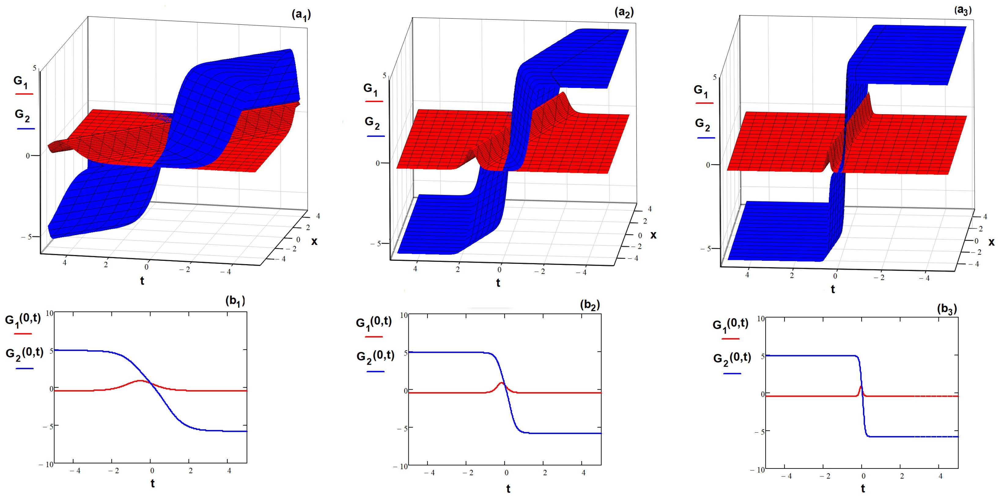
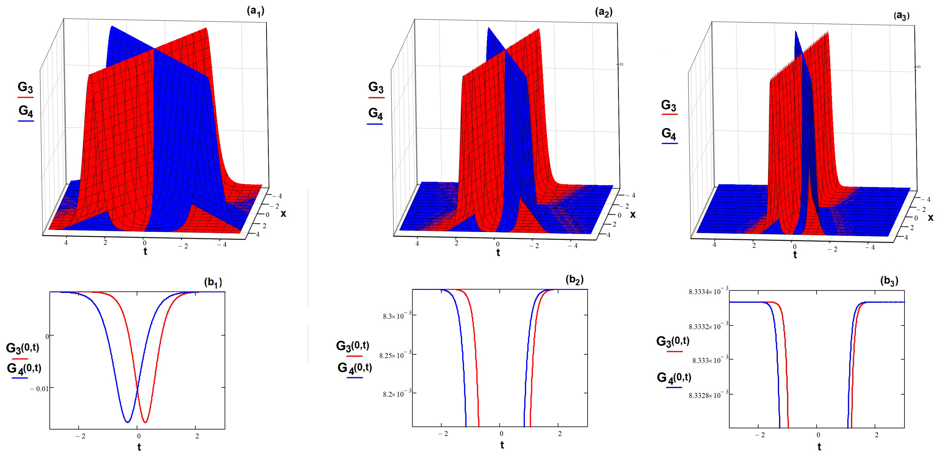
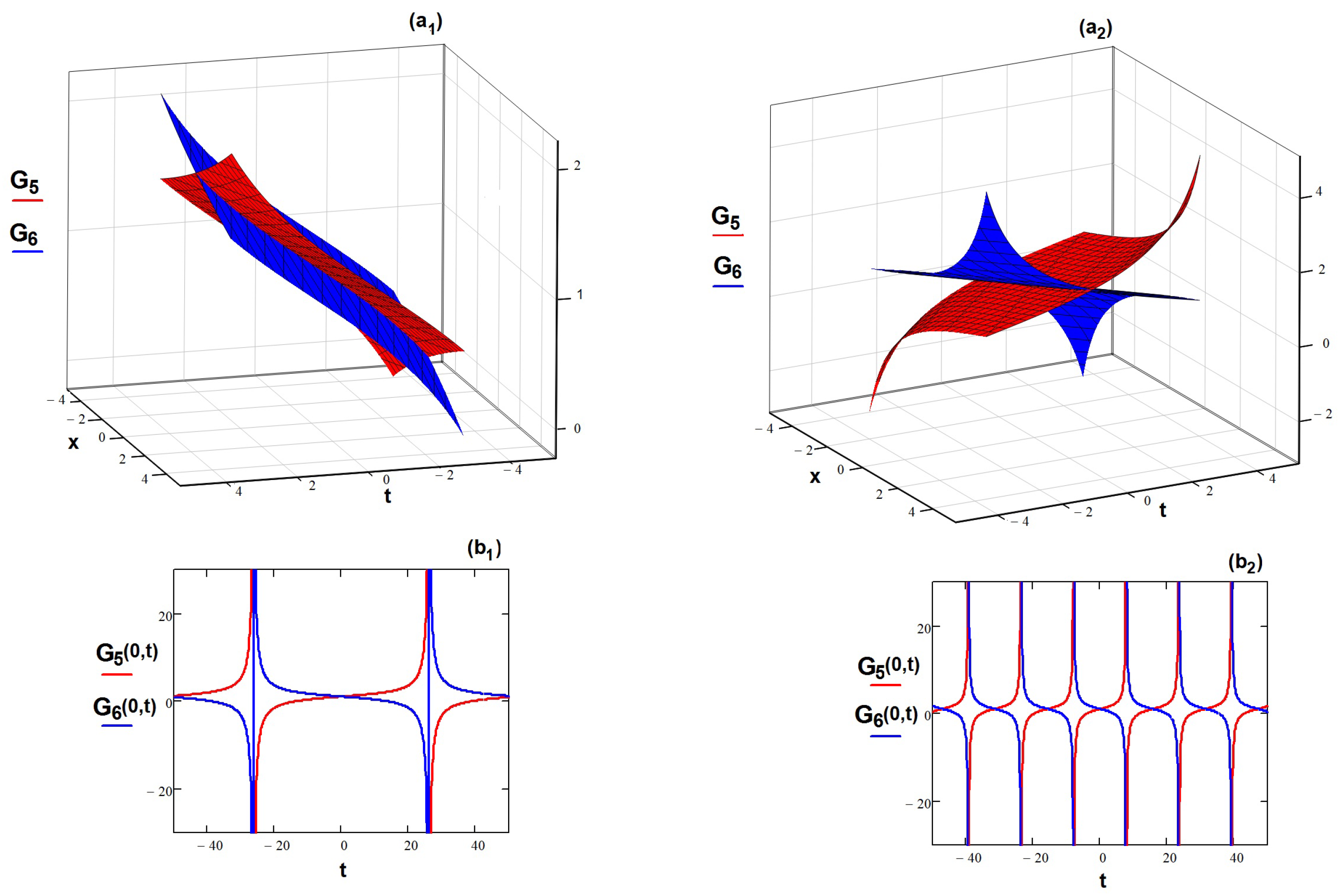
The TMCDG equation admits all of the same classes of solutions—hyperbolic, harmonic, and rational—as the unimodal Equation (3). As examples, we show that, using the Kudryashov expansion method, the TMCDG waves move in dual-mode, bright, and kink-wave shapes, while using the exponential expansion method, the motion could appear as having a dual t a n -periodic pattern. Of course, these are not the only solutions that can be generated; other solutions appear for different values of p and r.
-
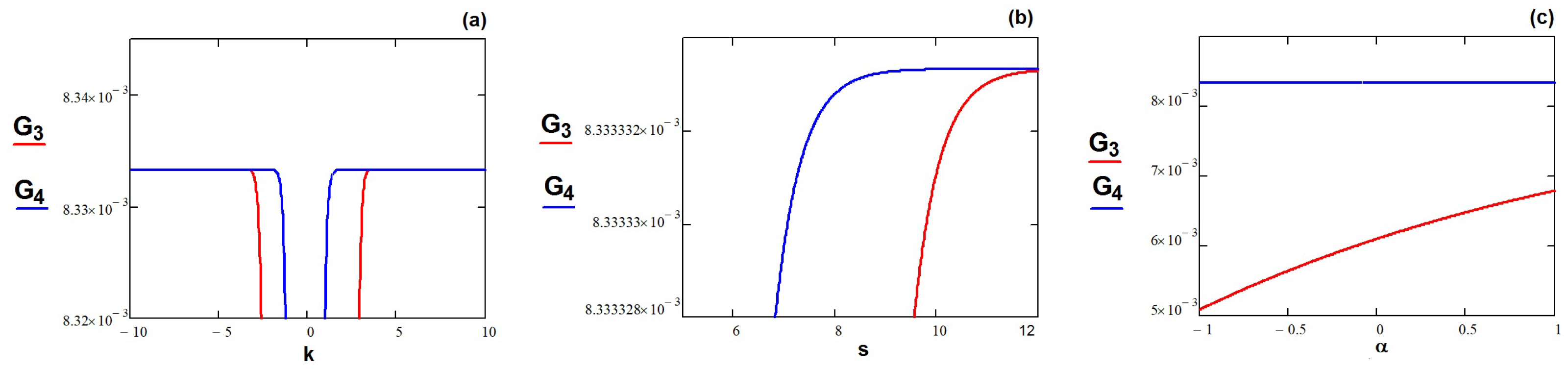
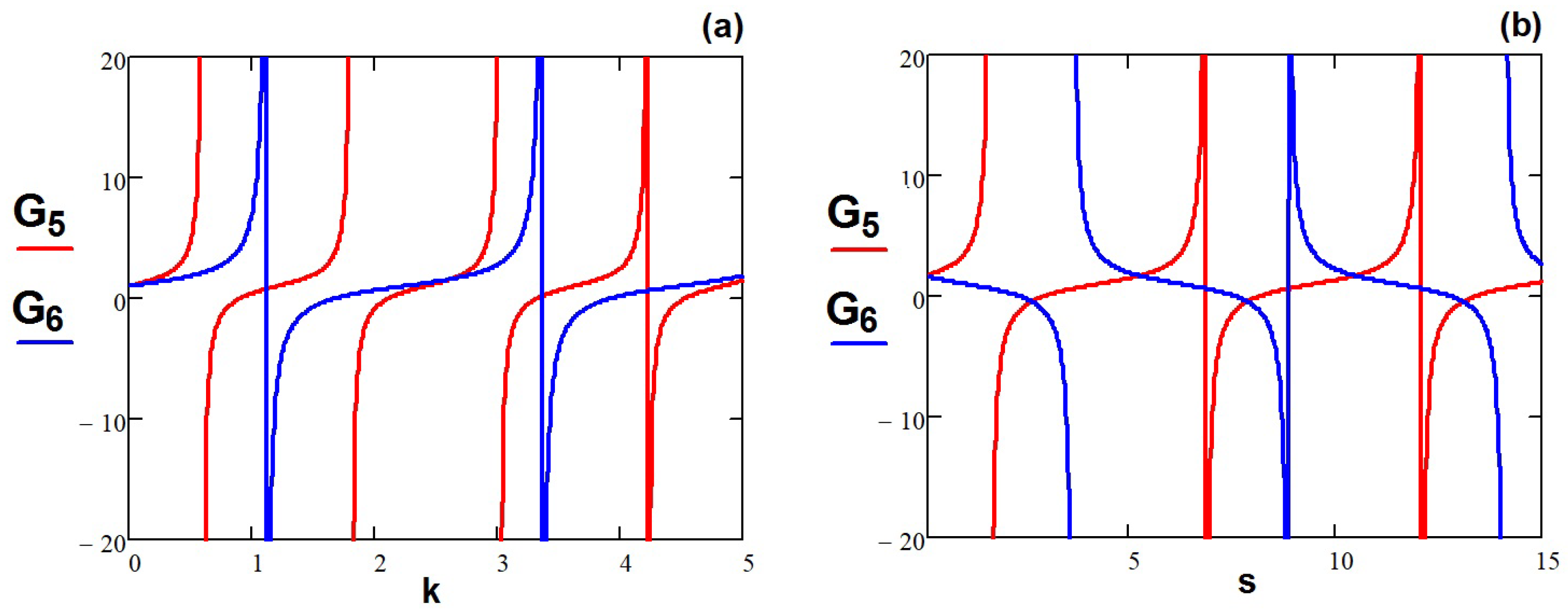
All solutions depend on the involved parameters, but the dependence is different. We note, for example, that the nonlinearity parameter β cannot take any value, but one depending on α . For G 1 , 2 ( x , t ) , the dependence is linear, while for G 3 , 4 ( x , t ) , a more complicated relation (17) appears. The periodic solution G 5 , 6 ( x , t ) asks for unitary values of the two parameters α and β , as the relation (22) shows.
-
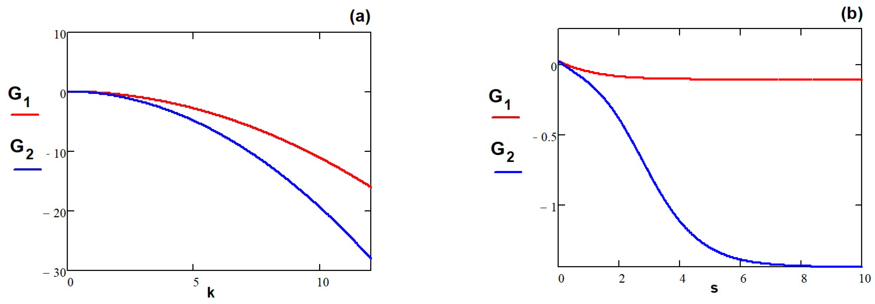
The influence of the main parameters (phase velocity s, wave number k and nonlinearity α ) is explained using the graphic representation of the solutions. Depending on their values, the parameters can increase or decrease the velocity of the dual waves.
The approach used here can be applied to any evolutionary NPDE of interest in mathematical physics and engineering, in order to achieve new dual-wave equations and their associated solutions. We will investigate in future work the possibility of extending the two-mode procedure to other higher-dimensional NPDEs or to integrodifferential systems [40], as well as trying to implement alternative techniques [41,42].

Author Contributions

The authors made an equal contribution to this work, with special involvements as follows: conceptualization, R.C. (Rodica Cimpoiasu); methodology, R.C. (Rodica Cimpoiasu); formal analysis, R.C. (Radu Constantinescu); writing—review and editing, R.C. (Radu Constantinescu) and R.C. (Rodica Cimpoiasu). All authors have read and agreed to the published version of the manuscript.

Funding

This research received no external funding.

Data Availability Statement

Not applicable.

Acknowledgments

The authors acknowledge the support offered by ICTP through the NT-03 Grant and by the University of Craiova.

Conflicts of Interest

The authors declare no conflict of interest.

References

  1. Zwillinger, D. Handbook of Differential Equations; Academic Press: New York, NY, USA, 1992. [Google Scholar]
  2. Korsunsky, S.V. Soliton solutions for a second order KdV equation. Phys. Lett. A 1994, 185, 174–176. [Google Scholar] [CrossRef]
  3. Wazwaz, A.M. A study on a two-wave mode Kadomtsev–Petviashvili equation: Conditions for multiple soliton solutions to exist. Math. Method Appl. Sci. 2017, 40, 4128–4133. [Google Scholar] [CrossRef]
  4. Wazwaz, A.M. Two wave mode higher-order modified KdV equations: Essential conditions for multiple soliton solutions to exist. Int. J. Numer. Method H. 2017, 27, 2223–2230. [Google Scholar] [CrossRef]
  5. Alquran, M.; Sulaiman, T.A.; Yusuf, A. Kink-soliton, singular-kink-soliton and singular-periodic solutions for a new two-mode version of the Burger-Huxley model: Applications in nerve fibers and liquid crystals. Opt. Quant. Electron. 2021, 53, 227. [Google Scholar] [CrossRef]
  6. Jaradat, I.; Alquran, M. Geometric perspectives of the two-mode upgrade of a generalized Fisher–Burgers equation that governs the propagation of two simultaneously moving waves. J. Comput. Appl. Math. 2022, 404, 113908. [Google Scholar] [CrossRef]
  7. Lee, C.T.; Liu, J.L. A Hamiltonian model and soliton phenomenon for a two-mode KdV equation. Rocky Mt. J. Math. 2011, 41, 1273–1289. [Google Scholar] [CrossRef]
  8. Lee, C.T.; Lee, C.C. On wave solutions of a weakly nonlinear and weakly dispersive two-mode wave system. Wave Random Complex 2013, 23, 56–76. [Google Scholar] [CrossRef]
  9. Wazwaz, A.M. Multiple soliton solutions and other exact solutions for a two-mode KdV equation. Math. Method Appl. Sci. 2017, 40, 2277–2283. [Google Scholar] [CrossRef]
  10. Xiao, Z.J.; Tian, B.; Zhen, H.L.; Chai, J.; Wu, X.Y. Multi-soliton solutions and Bcklund transformation for a two-mode KdV equation in a fluid. Wave Random Complex 2017, 27, 1–14. [Google Scholar] [CrossRef]
  11. Kumar, D.; Park, C.; Tamanna, N.; Paul, G.C.; Osman, M.S. Dynamics of two-mode Sawada-Kotera equation: Mathematical and graphical analysis of its dual-wave solutions. Results Phys. 2020, 19, 103581. [Google Scholar] [CrossRef]
  12. Jaradat, I.; Alquran, M.; Momani, S.; Biswas, A. Dark and singular optical solutions with dual-mode nonlinear Schrödinger’s equation and Kerr-law nonlinearity. Optik 2018, 172, 822–825. [Google Scholar] [CrossRef]
  13. Abu Irwaq, I.; Alquran, M.; Jaradat, I.; Baleanu, D. New dual-mode Kadomtsev–Petviashvili model with strong–weak surface tension: Analysis and application. Adv. Differ. Equ. 2018, 2018, 433. [Google Scholar] [CrossRef]
  14. Wazwaz, A.M. Two-mode Sharma-Tasso-Olver equation and two-mode fourth-order Burgers equation: Multiple kink solutions. Alex. Eng. J. 2018, 57, 1971–1976. [Google Scholar] [CrossRef]
  15. Alquran, M.; Jaradat, I.; Baleanu, D. Shapes and dynamics of dual-mode Hirota–Satsuma coupled KdV equations: Exact traveling wave solutions and analysis. Chin. J. Phys. 2019, 58, 49–56. [Google Scholar] [CrossRef]
  16. Wazwaz, A.M. Two-mode fifth-order KdV equations: Necessary conditions for multiple-soliton solutions to exist. Nonlinear Dynam. 2017, 87, 1685–1691. [Google Scholar] [CrossRef]
  17. Kumar, S.; Mohan, B.; Kumar, R. Lump, soliton, and interaction solutions to a generalized two-mode higher-order nonlinear evolution equation in plasma physics. Nonlinear Dyn. 2022, 110, 693–704. [Google Scholar] [CrossRef]
  18. Alquran, M.; Alhami, R. Convex-periodic, kink-periodic, peakon-soliton and kink bidirectional wave-solutions to new established two-mode generalization of cahn-allen equation. Results Phys. 2022, 34, 105257. [Google Scholar] [CrossRef]
  19. Cimpoiasu, R.; Pauna, A.S. Complementary wave solutions for the long-short wave resonance model via the extended trial equation method and the generalized Kudryashov method. Open Phys. 2018, 16, 419–426. [Google Scholar] [CrossRef]
  20. Ferdous, F.; Hafez, M.G.; Akther, S. Oblique traveling wave closed-form solutions to space-time fractional coupled dispersive long wave equation through the generalized exponential expansion method. Int. J. Comput. Math. 2022, 8, 142. [Google Scholar] [CrossRef]
  21. Babalic, C.N. Complete integrability and complex solitons for generalized Volterra system with branched dispersion. Int. J. Mod. Phys. B 2020, 34, 2050274. [Google Scholar] [CrossRef]
  22. Babalic, C.N. Integrable discretization of coupled Ablowitz-Ladik equations with branched dispersion. Rom. J. Phys. 2018, 63, 114. [Google Scholar]
  23. Cimpoiasu, R.; Constantinescu, R. Invariant solutions of the Eckhaus-Kundu model with nonlinear dispersion and non-Kerr nonlinearities. Wave Random Complex 2021, 31, 331–341. [Google Scholar] [CrossRef]
  24. Cimpoiasu, R.; Rezazadeh, H.; Florian, D.A.; Ahmad, H.; Nonlaopon, K.; Altanji, M. Symmetry reductions and invariant-group solutions for a two-dimensional Kundu-Mukherjee-Naskar model. Results Phys. 2021, 28, 104583. [Google Scholar] [CrossRef]
  25. Khater, M.M. Computational and numerical wave solutions of the Caudrey–Dodd–Gibbon equation. Heliyon 2023, 9, e13511. [Google Scholar] [CrossRef]
  26. Polat, M.; Oruç, Ö. A combination of Lie group-based high order geometric integrator and delta-shaped basis functions for solving Korteweg-de Vries (KdV) equation. Int. J. Geom. M. 2021, 18, 2150216. [Google Scholar] [CrossRef]
  27. Hu, X.B.; Li, Y. Some results on the Caudrey-Dodd-Gibbon-Kotera-Sawada equation. J. Phys. A-Math. Gen. 1991, 24, 3205. [Google Scholar] [CrossRef]
  28. Majeed, A.M.; Rafiq, V.; Kamran, M.; Abbas, M.; Inc, M. Analytical solutions of the fifth-order time fractional nonlinear evolution equations by the unified method. Mod. Phys. Lett. B 2022, 36, 2150546. [Google Scholar] [CrossRef]
  29. Ionescu, C. The sp(3) BRST Hamiltonian formalism for the Yang-Mills fields. Mod. Phys. Lett. A 2008, 23, 737–775. [Google Scholar] [CrossRef]
  30. Adeyemo, O.D.; Khalique, C.M. Lie group theory, stability analysis with dispersion property, new soliton solutions and conserved quantities of 3D generalized nonlinear wave equation in liquid containing gas bubbles with applications in mechanics of fluids, biomedical sciences and cell biology. Commun. Nonlinear Sci. 2023, 123, 107261. [Google Scholar]
  31. Márquez, A.P.; Bruzón, M.S. Lie point symmetries, traveling wave solutions and conservation laws of a non-linear viscoelastic wave equation. Mathematics 2021, 9, 2131. [Google Scholar] [CrossRef]
  32. Cimpoiasu, R. Conservation Laws and associated Lie symmetries for 2D Ricci flow model. Rom. J. Phys. 2013, 58, 519–528. [Google Scholar]
  33. Cimpoiasu, R. Multiple invariant solutions of the 3 D potential Yu–Toda–Fukuyama equation via symmetry technique. Int. J. Mod. Phys. B 2020, 34, 2050188. [Google Scholar] [CrossRef]
  34. Ionescu, C.; Constantinescu, R. Solving Nonlinear Second-Order Differential Equations through the Attached Flow Method. Mathematics 2022, 10, 2811. [Google Scholar] [CrossRef]
  35. Henneaux, M.; Teitelboim, C. Quantization of Gauge Systems; Princeton University Press: Princeton, NJ, USA, 1992. [Google Scholar]
  36. Alquran, M. Optical bidirectional wave-solutions to new two-mode extension of the coupled KdV–Schrodinger equations. Opt. Quant. Electron. 2021, 53, 588. [Google Scholar] [CrossRef]
  37. Jaradat, I.; Alquran, M. Construction of solitary two-wave solutions for a new two-mode version of the Zakharov-Kuznetsov equation. Mathematics 2020, 8, 1127. [Google Scholar] [CrossRef]
  38. Akbar, M.A.; Akinyemi, L.; Yao, S.W.; Jhangeer, A.; Rezazadeh, H.; Khater, M.M.; Ahmad, H.; Inc, M. Soliton solutions to the Boussinesq equation through sine-Gordon method and Kudryashov method. Results Phys. 2021, 25, 104228. [Google Scholar] [CrossRef]
  39. Akbar, M.A.; Ali, N.H.M.; Tanjim, T. Outset of multiple soliton solutions to the nonlinear Schrodinger equation and the coupled Burgers equation. J. Phys. Commun. 2019, 3, 095013. [Google Scholar] [CrossRef]
  40. Vijayakumar, V.; Nisar, K.S.; Chalishajar, D.; Shukla, A.; Malik, M.; Alsaadi, A.; Aldosary, S.F. A note on approximate controllability of fractional semilinear integrodifferential control systems via resolvent operators. Fractal Fract 2022, 6, 73. [Google Scholar] [CrossRef]
  41. Xu, G.Q.; Wazwaz, A.M. Bidirectional solitons and interaction solutions for a new integrable fifth-order nonlinear equation with temporal and spatial dispersion. Nonlinear Dyn. 2020, 101, 581–595. [Google Scholar] [CrossRef]
  42. Cimpoiasu, R.; Cimpoiasu, V.; Constantinescu, R. Nonlinear dynamical systems in various space-time dimensions. Rom. J. Phys. 2010, 55, 25–35. [Google Scholar]
Figure 1. The 3 D plots of the dual-wave solutions G 1 ( x , t ) (red color) and G 2 (blue color) given by (19), for α = 0.8 , β = 1 , d = 3 , k = 2 , and (a 1 ) s = 1 , (a 2 ) s = 3 , (a 3 ) s = 10 . The 2 D cross-sections of (a 1 a 3 ) at x = 0 are plotted in (b 1 b 3 ).
Axioms 12 00619 g001
Figure 2. (a) The dependence on k when s = 1 , d = 3 , α = 0.8, β = 1 , (b) the dependence on s when k = 1 , d = 3 , α = 0.8, β = 1 of the motion of the two-mode waves G 1 ( x , t ) (red color) and G 2 ( x , t ) (blue color) given by (19) for x = 1 , t = 1 .
Axioms 12 00619 g002
Figure 3. (a) The 3 D plots of the dual-wave solutions G 3 ( x , t ) (red color) and G 4 ( x , t ) (blue color) given by (20) for a 2 = 0.1, d = 3 , k = 2 , α = 0.2 and variable s. Three phase velocities were considered: (a 1 ) s = 1 , (a 2 ) s = 3 , and (a 3 ) s = 5 . The 2 D cross-sections of (a 1 a 3 ) at x = 0 are plotted in (b 1 b 3 ).
Axioms 12 00619 g003
Figure 4. The effect on the motion of the two-mode waves G 3 ( x , t ) (red color) and G 4 ( x , t ) (blue color) given by (20), at x = 3 , t = 1 , of (a) wave number k when s = 5 , α = 0.2, a 2 = 0.1, d = 3 ; (b) phase velocity s when k = 2 , α = 0.2 , a 2 = 0.1, d = 3 ; and (c) the nonlinearity parameter α when k = 2 , s = 5 , a 2 = 0.1, d = 3 .
Axioms 12 00619 g004
Figure 5. The 3 D graphs of G 5 ( x , t ) (red color) and G 6 (blue color) given by (24), with α = β = 1 , ρ 0 = 1 , ρ 2 = 4 , k = 0.1, p = 0.5, r = 2 , q = 0 , and the phase velocities: (a 1 ) s = 0.3, (a 2 ) s = 1 . The 2 D graphs of (a 1 ,a 2 ) at x = 0 are plotted in (b 1 ,b 2 ).
Axioms 12 00619 g005
Figure 6. The effect on the motion of the two-mode waves G 5 ( x , t ) (red color) and G 6 ( x , t ) (blue color) given by (24) at x = 3 , t = 3 , of (a) the wave number k when α = β = 1 , s = 0.3, ρ 0 = 1 , ρ 2 = 4 , p = 0.5, r = 2 , q = 0 ; (b) the phase velocity parameter s when ρ 0 = 1 , ρ 2 = 4 , k = 0.1, p = 0.5, r = 2 , q = 0 .
Axioms 12 00619 g006
Disclaimer/Publisher’s Note: The statements, opinions and data contained in all publications are solely those of the individual author(s) and contributor(s) and not of MDPI and/or the editor(s). MDPI and/or the editor(s) disclaim responsibility for any injury to people or property resulting from any ideas, methods, instructions or products referred to in the content.

