An Efficient Jarratt-Type Iterative Method for Solving Nonlinear Global Positioning System Problems

Abstract

The global positioning system (GPS) is a satellite navigation system that determines locations. Whenever the baseline satellites are serviced or deactivated, the Space Force often flies more than 24 GPS satellites to maintain coverage. The additional satellites are not regarded as a part of the core constellation but may improve the performance of the GPS. In this study of GPS models, we solved various problems. We examined each set of four satellites separately. Advancements in computer softwares have made computations much more precise. We can use iterative methods to solve GPS problems. Iterative schemes for solving nonlinear equations have always been of great importance because of their applicability to real-world problems. This paper involves the development of an efficient family of sixth-order Jarratt-type iterative schemes for analyzing nonlinear global positioning systems.

1. Introduction

In the field of numerical analysis, developing fast and cost-effective iterative schemes to approximate the solutions for nonlinear systems of equations is a noteworthy and demanding task. The importance of this subject has been the incentive behind the development of many numerical iterative techniques [1,2,3,4,5,6,7,8,9]. Generally, higher-order iterative schemes are developed for scalar equations, which are then extended to the multidimensional case conserving the order of convergence.

However, not all methods are extendable in this way. Recently, researchers have proposed sixth-order iterative methods using weight functions and parameters [10,11,12,13]. We typically turn to their numerical solutions because exact nonlinear solutions are rarely available. There are a wide range of nonlinear phenomena in GPS problems. Awange and Grafarend [14] presented alternative algebraic procedures using a multipolynomial resultant and Groebner basis to solve the GPS navigation problems. Pachter and Nguyenan [15] proposed an efficient GPS position determination two-step algorithm. In step one, the linear regression problem is solved and the result is updated based on a single nonlinear measurement equation. Instead of the five iterations generally required by the current conventional iterative least-squares (ILS) technique, just two or three iterations are needed in step two. For situations in which two or more GPS receivers are active at once, Yang [16] developed a highly compatible algebraic positioning method using a noniterative approach that uses a direct solution to the double-difference pseudorange equations. Li et al. [17] analyzed a new GPS positioning technique using direct linearization. Ko and Choi [18] proposed mathematical methods for two-dimensional positioning based on a GPS pseudorange technique. Jwoa et al. [19] used the iterative least-absolute-deviation approach to solve GPS navigation problems. Different methods [20,21,22,23,24] have been proposed to find solutions to GP problems. In many modern GPS devices, the Newton–Raphson method is primarily used [21].

Astronavigation systems such as GPS facilitate users to obtain worldwide coverage. This service is attainable around the clock by users. At least 24 satellites are above the Earth’s surface at an altitude of approximately 20,000 km in the shape of a circular orbital constellation. The GPS can be categorized (Figure 1) into three major segments:

(1)

The space segment comprises a cluster of 24 Navstar satellites;

(2)

The control segment is composed of a network of tracking and governing equipment;

(3)

The user segment receives, interprets, and processes the GPS satellite data with a specially designed variety of navigational radio receivers.

These three segments deliver extensive features, validity, and authenticity.

Figure 1. NAVSTAR/GPS major segments.

A settlement between user demand, commercial constraints, and technical feasibility has always been expressed by the configuration of GPS satellites. Making decisions about where to put the satellites, how many there should be, how high, and how close is difficult. The goal of the constellation is to provide an efficient operating system for an extensive class of users. In early GPS models, each orbit contained eight satellites uniformly distributed 45 degrees apart. The angle of inclination was usually set to 63 degrees with an orbital period of 11 h and 58 min.

The mechanics of each satellite play a vital role in determining the optimal GPS satellite configuration. Scientists and researchers must consider the reliability of parts in a satellite (Figure 2) by taking into account various constraints. The atomic clock is an essential part of a satellite. There are three or four cesium or rubidium atomic clocks in each GPS satellite. Atomic clocks show the most accurate time. The atomic clock is highly precise but, at the same time, it is not ideal because of the high cost and clock errors. Each day, the clock error in a satellite amounts to about 8.64 to 17.28 nanoseconds. For the maintenance of satellites and their proper functioning, the operational control segment (OCS) is responsible. It predicts satellite locations by tracking the GPS satellites. Recent and corrected navigation messages from each satellite are updated by the OCS once a day or depending on the need. The messages are based on information about each satellite’s position. Monitoring stations, the ground antennas, and the master control station (MCS) are the components of the control segment of the GPS (Figure 3).

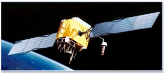
Figure 2. Navstar GPS IIF.

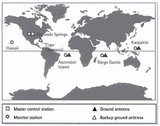
Figure 3. GPS master control center and monitoring stations.

Measurement of Pseudorange

Various problems had to be solved while testing and studying the GPS models. For example, each set of four satellites had to be examined separately. Current advancements in computer software have made computations much more precise. Now, satellites are fixed in six orbital planes at 60 degrees apart with four satellites in each plane (Figure 4).

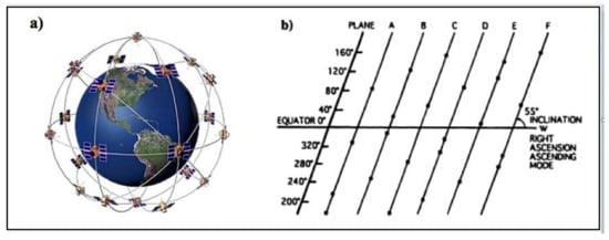
Figure 4. GPS satellite constellation: (a) orbital planes; (b) satellite positions on the orbital planes.

The nonlinear pseudorange equations used to determine the user position from the satellite swarm are computed with higher precision. We changed the coordinates into a spherical system to integrate the user position. We could determine unknown user positions by estimating the distance from the specified position in space. The three distances are required in determining a two-dimensional user position, as displayed in Figure 5. By using two satellites, two possible solutions can be obtained where both of the circles intersect.

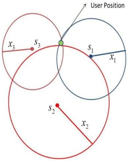
Figure 5. Two-dimensional user position.

For a three-dimensional case, we take four satellites with four distances, as can be viewed in Figure 6 (for more detail, see [25]).

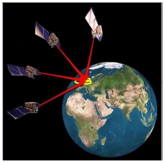
Figure 6. Three-dimensional user position.

The pseudorange is known as a common bias that is measured by the receiver range of the satellites. The pseudorange, $\zeta$, is the distance between the user and the satellite geometric range multiplied by the velocity of light, c. The mathematical form is given as:

$${\zeta }_i=\sqrt{{(x_{1sati}-x_{1user})}^2+{(x_{2sati}-x_{2user})}^2+{(x_{3sati}-x_{3user})}^2}+c\Delta t_i.$$

(1)

where ${\zeta }_i$, $x_{1sati}$, $x_{2sati}$, and $x_{3sati}$ are known and $x_{1user}$, $x_{2user}$, $x_{3user}$, and $\Delta t_i$ are unknowns. As $\Delta t_i$ is the true bias, as has been estimated [26,27,28], it is sufficient to consider the coordinates of four satellites to figure out the position values. Thus, for i = 1, 2, …, n $\in N$, the equations are given as:

$${\zeta }_i=p_i+c\Delta t_i,$$

where

$$p_i=\sqrt{{(x_{1sati}-x_{1user})}^2+{(x_{2sati}-x_{2user})}^2+{(x_{3sati}-x_{3user})}^2}.$$

2. Development of Method

We developed a new sixth-order method by modifying the second step of the method from [29] for solving nonlinear systems of equations.

Derivation of the Scheme

For our multidimensional scheme, we let $G:\mu \subset {\mathbb{R}}^n\to {\mathbb{R}}^n$ be a multivariate vector-valued function; then, we define

$$\begin{array}{ccc}\hfill w^{\left(\alpha \right)}& =& s^{\left(\alpha \right)}-\frac{2}{3}{\left(G^{\prime }\left(s^{\left(\alpha \right)}\right)\right)}^{-1}G\left(s^{\left(\alpha \right)}\right),\hfill \\ \hfill z^{\left(\alpha \right)}& =& s^{\left(\alpha \right)}-\Omega \left(u^{(\alpha )}\right){\left(G^{\prime }\left(s^{\left(\alpha \right)}\right)\right)}^{-1}G\left(s^{\left(\alpha \right)}\right),\hfill \\ \hfill s^{\left(\alpha +1\right)}& =& z^{\left(\alpha \right)}-\varphi \left(v^{(\alpha )}\right){\left(G^{\prime }\left(s^{\left(\alpha \right)}\right)\right)}^{-1}G\left(z^{\left(\alpha \right)}\right),\hfill \end{array}$$

(2)

with

$$u^{(\alpha )}={\left(G^{\prime }\left(w^{\left(\alpha \right)}\right)\right)}^{-1}{G}^{\prime }\left(s^{\left(\alpha \right)}\right),$$

$$v^{(\alpha )}={\left(G^{\prime }\left(s^{\left(\alpha \right)}\right)\right)}^{-1}{G}^{\prime }\left(w^{\left(\alpha \right)}\right).$$

where $\Omega ,\sigma :A_{n\times n}(\mathbb{R})\to \Gamma ({\mathbb{R}}^n),$ with $A_{n\times n}$ being the set of $n\times n$ matrices and $\Gamma ({\mathbb{R}}^n)$ being the set of linear operators from ${\mathbb{R}}^n$ to ${\mathbb{R}}^n.$

Theorem 1.

Let us suppose that $G:\mu \subseteq R^n\to R^n$ is a sufficiently Frechet-differentiable function in a closed neighborhood ω containing the simple root Υ. Let $G^{\prime }(s)$ be continuous and nonsingular at Υ and the initial guess for $s^{(0)}$ be close to the root Υ; then, Equation (2) becomes a sixth-order convergent numerical scheme for the following conditions:

$$\Omega (I)=I,{\Omega }^{\prime }(I)=\frac{3}{4}I,{\Omega }^{″}(I)=\frac{3}{4}I,$$

$$\parallel {\Omega }^{‴}(I)\parallel <\infty ,$$

$$\varphi (I)=I,{\varphi }^{\prime }(I)=-\frac{3}{2}I,\parallel {\varphi }^{″}(I)\parallel <\infty .$$

Proof. 

We take $e^{(\alpha )}$ = $s^{(k)}-\mathsf{{\rm Y}}$ as the error in the $\alpha$th iteration. The Taylor’s series expansion of the function $G(s^{(k)})$ and its first-order derivative $G^{\prime }(s^{(k)})$ with the assumption $\parallel G^{\prime }(\mathsf{{\rm Y}})\parallel \ne 0$ leads us to:

$$\begin{array}{ccc}\hfill G(s^{(\alpha )})& =& G^{\prime }(\mathsf{{\rm Y}})[e^{(\alpha )}+d_2{(e^{(\alpha )})}^2+d_3{(e^{(\alpha )})}^3+d_4{(e^{(\alpha )})}^4+d_5{(e^{(\alpha )})}^5+d_6{(e^{(\alpha )})}^6\hfill \end{array}$$

$$\begin{array}{c}\hfill +O({(e^{(\alpha )})}^7)],\end{array}$$

(3)

where

$$d_i=\frac{1}{i!}{\left[G^{\prime }(\mathsf{{\rm Y}})\right]}^{-1}{G}^i(\mathsf{{\rm Y}}),i=2,3,\dots$$

and

$$\begin{array}{ccc}\hfill G^{\prime }(s^{(\alpha )})& =& G^{\prime }(\mathsf{{\rm Y}})[I+2d_2{e}^{(\alpha )}+3d_3{(e^{(\alpha )})}^2+4d_4{(e^{(\alpha )})}^3+5d_5{(e^{(\alpha )})}^4+6d_6{(e^{(\alpha )})}^5\hfill \end{array}$$

$$\begin{array}{c}\hfill +O({(e^{(\alpha )})}^6)],\end{array}$$

as $G^{\prime }(s^{(\alpha )})$ and ${(G^{\prime }(s^{(\alpha )}))}^{-1}$ are $n\times n$ matrices and I is the $n\times n$ identity matrix. We found ${(G^{\prime }(s^{(\alpha )}))}^{-1}$ by choosing

$$E=-(2d_2{e}^{(\alpha )}+3d_3{(e^{(\alpha )})}^2+4d_4{(e^{(\alpha )})}^3+5d_5{(e^{(\alpha )})}^4+6d_6{(e^{(\alpha )})}^5+O({(e^{(\alpha )})}^6)),$$

from the relation

$${(I-E)}^{-1}=I+E+E^{(2)}+E^{(3)}+E^{(4)}+E^{(5)}+O(E^{(6)}),$$

Thus, we obtain the inversion of $G^{\prime }(s^{(\alpha )})$ as

$$\begin{array}{ccc}\hfill {(G^{\prime }(s^{(\alpha )}))}^{-1}& =& [I-2d_2{e}^{(\alpha )}+(4d_2^2-3d_3){(e^{(\alpha )})}^2+(-8d_2^3+6d_2{d}_3+6d_3{d}_2-4d_4){(e^{(\alpha )})}^3\hfill \end{array}$$

$$\begin{array}{ccc}& & +(16d_2^4+9d_3^2-12d_2^2{d}_3-12d_2{d}_3{d}_2-12d_3{d}_2^2+8d_2{d}_4+8d_4{d}_2-5d_5){(e^{(\alpha )})}^4\hfill \end{array}$$

$$\begin{array}{c}\hfill +O({(e^{(\alpha )})}^5)].\end{array}$$

(4)

By using Equations (3) and (4) in the first step of Equation (2) and applying Taylor’s series expansion, we get

$$\begin{array}{ccc}\hfill w^{(\alpha )}-\mathsf{{\rm Y}}& =& s^{(\alpha )}-\mathsf{{\rm Y}}-\frac{2}{3}{(G^{\prime }(s^{(\alpha )}))}^{-1}G\left(s^{(\alpha )}\right)\hfill \\ & =& \frac{1}{3}{e}^{(\alpha )}+\frac{2}{3}{d}_2{(e^{(\alpha )})}^2+(\frac{4}{3}{d}_3-\frac{4}{3}{d}_2^2){(e^{(\alpha )})}^3+(2d_4-\frac{14}{3}{d}_2{d}_3+\frac{8}{3}{d}_2^3){(e^{(\alpha )})}^4\hfill \end{array}$$

$$\begin{array}{c}\hfill +{\displaystyle \sum _{i=5}^6}{A}_i{(e^{(\alpha )})}^i+O({(e^{(\alpha )})}^7),\end{array}$$

$$A_i=A_i(d_2,d_3,\dots d_6),5⩽i⩽6.$$

Furthermore, $G^{\prime }(w^{(\alpha )})={\left.G^{\prime }(s^{(\alpha )})\right|}_{e^{(\alpha )}\to (w^{(\alpha )}-\mathsf{{\rm Y}})}$ is given by

$$\begin{array}{ccc}\hfill G^{\prime }(w^{(\alpha )})& =& G^{\prime }(\mathsf{{\rm Y}})[I+\frac{2}{3}{d}_2{e}^{(\alpha )}+\frac{1}{3}(4d_2^2+d_3){(e^{(\alpha )})}^2+(\frac{8}{3}{d}_2{d}_3-\frac{8}{3}{d}_2^3+\frac{4}{27}{d}_4){(e^{(\alpha )})}^3\hfill \\ & & +{\displaystyle \sum _{i=4}^5}{B}_i{(e^{(\alpha )})}^i]+O({(e^{(\alpha )})}^7),\hfill \end{array}$$

where

$$B_i=B_i(d_2,d_3,\dots d_6),4⩽i⩽5.$$

Now

$$u^{(\alpha )}={(G^{\prime }(w^{(\alpha )}))}^{-1}{G}^{\prime }(s^{(\alpha )}),$$

$$\begin{array}{ccc}\hfill u^{(\alpha )}& =& I+\frac{4}{3}{d}_2{e}^{(\alpha )}+(\frac{8}{3}{d}_3-\frac{20}{9}{d}_2^2){(e^{(\alpha )})}^2+{\displaystyle \sum _{i=3}^5}{D}_i{(e^{(\alpha )})}^i+O({(e^{(\alpha )})}^7).\hfill \end{array}$$

(5)

where

$$D_i=D_i(d_2,d_3,\dots d_6),3⩽i⩽5.$$

Moreover, $\Omega (u^{(\alpha )})$ is given by

$$\begin{array}{ccc}\hfill \Omega (u^{(\alpha )})& =& \Omega (I)+\frac{4}{3}{\Omega }^{\prime }(I)d_2{e}^{(\alpha )}+(\frac{8}{3}{\Omega }^{\prime }(I)d_3-\frac{20}{9}{\Omega }^{\prime }(I)d_2^2+\frac{8}{9}{\Omega }^{″}(I)d_2^2){(e^{(\alpha )})}^2\hfill \\ & & +{\displaystyle \sum _{i=3}^5}{H}_i{(e^{(\alpha )})}^i+O({(e^{(\alpha )})}^6),\hfill \end{array}$$

where

$$H_i=H_i(d_2,d_3,\dots d_6,{\Omega }^{\prime }(I),{\Omega }^{″}(I),{\Omega }^{‴}(I){\Omega }^{iv}(I)),3⩽i⩽5.$$

Considering the second step of Equation (2) as

$$\begin{array}{ccc}\hfill z^{(\alpha )}-\mathsf{{\rm Y}}& =& s^{(\alpha )}-\mathsf{{\rm Y}}-\Omega (u^{(\alpha )}){\left(G^{{}^{\prime }}\left(s^{\left(\alpha \right)}\right)\right)}^{-1}G\left(s^{\left(\alpha \right)}\right)\hfill \end{array}$$

$$\begin{array}{c}\hfill =(I-\Omega (I))e^{(\alpha )}-\frac{1}{3}{d}_2(-3\Omega (I)+4{\Omega }^{\prime }(I)){(e^{(\alpha )})}^2+(2\Omega (I)d_3-\frac{8}{3}{\Omega }^{\prime }(I)d_3+\frac{32}{9}{\Omega }^{\prime }(I)d_2^2\\ \hfill -\frac{8}{9}{\Omega }^{″}(I)d_2^2-2\Omega (I)d_2^2){(e^{(\alpha )})}^3+{\displaystyle \sum _{i=4}^6}{H}_i{(e^{(\alpha )})}^i+O({(e^{(\alpha )})}^7),\end{array}$$

(6)

and taking the conditions for weight functions

$$\Omega (I)=I,{\Omega }^{\prime }(I)=\frac{3}{4}I,{\Omega }^{\prime }(I)=\frac{3}{4}I,\parallel {\Omega }^{‴}(I)\parallel <\infty ,$$

Equation (6) becomes

$$\begin{array}{ccc}\hfill z^{(\alpha )}& =& (-d_2{d}_3+\frac{1}{9}{d}_4+\frac{13}{9}{d}_2^3-\frac{32}{81}{\Omega }^{‴}(I)d_2^3){(e^{(\alpha )})}^4+{\displaystyle \sum _{i=5}^6}{J}_i{(e^{(\alpha )})}^i+O({(e^{(\alpha )})}^7),\hfill \end{array}$$

where

$$J_i=J_i(d_2,d_3,\dots d_6,{\Omega }^{‴}(I),{\Omega }^{iv}(I)),5⩽i⩽6.$$

Moreover, we have $G(z^{(\alpha )})={\left.G(s^{(\alpha )})\right|}_{e^{(\alpha )}\to (z^{(\alpha )}-\mathsf{{\rm Y}})}$

$$\begin{array}{ccc}\hfill G(z^{(\alpha )})& =& G^{\prime }(\mathsf{{\rm Y}})(-d_2{d}_3+\frac{1}{9}{d}_4+\frac{13}{9}{d}_2^3-\frac{32}{81}{\Omega }^{‴}(I)d_2^3){(e^{(\alpha )})}^4+{\displaystyle \sum _{i=5}^6}{J}_i{(e^{(\alpha )})}^i\hfill \\ & & +O({(e^{(\alpha )})}^7).\hfill \end{array}$$

(7)

Furthermore,

$$v^{(\alpha )}={(G^{\prime }(s^{(\alpha )}))}^{-1}{G}^{\prime }(w^{(\alpha )})$$

$$\begin{array}{ccc}\hfill v^{(\alpha )}& =& I-\frac{4}{3}{d}_2{e}^{(\alpha )}+(-\frac{8}{3}{d}_3+4d_2^2){(e^{(\alpha )})}^2+(-\frac{104}{27}{d}_4+\frac{40}{3}{d}_2{d}_3-\frac{32}{3}{d}_2^3){(e^{(\alpha )})}^3\hfill \\ & & +{\displaystyle \sum _{i=4}^5}{K}_i{(e^{(\alpha )})}^i+O({(e^{(\alpha )})}^6),\hfill \end{array}$$

where

$$K_i=K_i(d_2,d_3,\dots d_6),4⩽i⩽5.$$

Similarly, $\varphi (v^{(\alpha )})$ is given as

$$\varphi (v^{(\alpha )})=\varphi (I)-\frac{4}{3}{\varphi }^{\prime }(I)d_2{e}^{(\alpha )}+(-\frac{8}{3}{\varphi }^{\prime }(I)d_3+4{\varphi }^{\prime }(I)d_2^2+\frac{8}{9}{\varphi }^{″}(I)d_2^2){(e^{(\alpha )})}^2+{\displaystyle \sum _{i=3}^5}{L}_i{(e^{(\alpha )})}^i$$

$$+O({(e^{(\alpha )})}^6),$$

(8)

where

$$L_i=L_i(d_2,d_3,\dots d_6,\varphi (I),{\varphi }^{\prime }(I),{\varphi }^{‴}(I),{\varphi }^{iv}(I)),3⩽i⩽5.$$

Finally, using Equations (4), (7) and (8) in last step of Equation (2) gives

$$\begin{array}{ccc}\hfill e^{(\alpha +1)}& =& (-d_2{d}_3+\frac{1}{9}{d}_4+\frac{13}{9}{d}_2^3-\frac{32}{81}{\Omega }^{‴}(I)d_2^3-\frac{1}{9}\varphi (I)d_4+\varphi (I)d_2{d}_3-\frac{13}{9}{d}_2^3\varphi (I)+\hfill \\ & & \frac{32}{81}\varphi (I){\Omega }^{‴}(I)d_2^3){(e^{(\alpha )})}^4+{\displaystyle \sum _{i=5}^6}{M}_i{(e^{(\alpha )})}^i+O({(e^{(\alpha )})}^6),\hfill \end{array}$$

(9)

where

$$M_i=M_i(d_2,d_3,\dots d_6,{\Omega }^{‴}(I),{\Omega }^{iv}(I),{\Omega }^v(I),\varphi (I),{\varphi }^{\prime }(I)),5⩽i⩽6.$$

It is apparent that, taking the following condition for the weight function

$$\varphi (I)=I,$$

Equation (9) becomes

$$\begin{array}{ccc}\hfill e^{(\alpha +1)}& =& (-\frac{4}{3}{\varphi }^{\prime }(I)d_3{d}_2^2+\frac{4}{27}{\varphi }^{\prime }(I)d_2{d}_4+\frac{52}{27}{\varphi }^{\prime }(I)d_2^4-\frac{128}{243}{\varphi }^{\prime }(I){\Omega }^{‴}(I)d_2^4\hfill \\ & & -2d_3{d}_2^2+\frac{2}{9}{d}_2{d}_4+\frac{26}{9}{d}_2^4-\frac{64}{81}{\Omega }^{‴}(I)d_2^4){(e^{(\alpha )})}^5+{\displaystyle \sum _{i=5}^6}{W}_i{(e^{(\alpha )})}^i\hfill \end{array}$$

$$\begin{array}{c}\hfill +O({(e^{(\alpha )})}^7),\end{array}$$

(10)

where

$$W_i=W_i(d_2,d_3,\dots d_6,{\Omega }^{‴}(I),{\Omega }^{iv}(I),{\Omega }^v(I),{\varphi }^{\prime }(I),{\varphi }^{″}(I)),5⩽i⩽6.$$

We get the fifth-order scheme, which forces us to choose

$${\varphi }^{\prime }(I)=-\frac{3}{2}I,\parallel {\varphi }^{″}(I)\parallel <\infty ,$$

to obtain the following error expression from Equation (10)

$$\begin{array}{ccc}\hfill e^{(\alpha +1)}& =& \frac{1}{729}(-54d_2^2+9d_3+8{\varphi }^{″}(I)d_2^2)(81d_2{d}_3-117d_2^3+32{\Omega }^{‴}(I)d_2^3-9d_4){(e^{(\alpha )})}^6\hfill \end{array}$$

$$\begin{array}{c}\hfill +O({(e^{(\alpha )})}^7).\end{array}$$

Thus, the error analysis indicates that the proposed scheme (Equation (2)) approaches the sixth-order of convergence. It completes the proof. □

Next, we consider a few particular cases of our presented scheme (Equation (2)) as follows.

Case one: Let us take $\Omega (u^{(\alpha )})$ and $\varphi (v^{(k)})$ as rational and polynomials operators as follows:

$$\Omega (u^{(\alpha )})=a_{0}I{\left(I+a_1{u}^{(\alpha )}+a_2{(u^{(\alpha )})}^2\right)}^{-1},$$

$$\varphi (v^{(\alpha )})=b_{0}I+b_1{v}^{(\alpha )}+b_2{(v^{(\alpha )})}^2,$$

and

$$a_0=\frac{16}{31}I,a_1=-\frac{18}{31}I,a_2=\frac{3}{31}I,$$

$$b_0=\frac{5}{2}I+b_2,b_1=-\frac{3}{2}I-2b_2,b_2=b_2,$$

such that, for $b_2=3I$,

$$b_0=\frac{11}{2}I,b_1=-\frac{15}{2}I.$$

Thus, we have a sixth-order scheme titled $F{S}_1$, which is presented as:

$$\begin{array}{ccc}\hfill w^{(\alpha )}& =& s^{(\alpha )}-\frac{2}{3}{\left(G^{\prime }\left(s^{\left(\alpha \right)}\right)\right)}^{-1}G\left(s^{\left(\alpha \right)}\right),\hfill \\ \hfill z^{(\alpha )}& =& s^{(\alpha )}-16I{\left(31I-18u^{(\alpha )}+3{(u^{(\alpha )})}^2\right)}^{-1}{\left(G^{\prime }\left(s^{\left(\alpha \right)}\right)\right)}^{-1}G\left(s^{\left(\alpha \right)}\right),\hfill \\ \hfill s^{(\alpha +1)}& =& z^{(\alpha )}-\left(\frac{11}{2}I-\frac{15}{2}{v}^{(\alpha )}+3{(v^{(\alpha )})}^2\right){\left(G^{\prime }\left(s^{\left(\alpha \right)}\right)\right)}^{-1}G\left(z^{\left(\alpha \right)}\right).\hfill \end{array}$$

(11)

Case two: If the weight functions $\Omega (u^{(\alpha )})$ and $R(v^{(\alpha )})$ are taken as:

$$\Omega (u^{(\alpha )})=a_{0}I{\left(I+a_1{u}^{(\alpha )}+a_2{(u^{(\alpha )})}^2\right)}^{-1},$$

$$\varphi (v^{(\alpha )})=b_{0}I{\left(I+b_1{v}^{(\alpha )}+b_2{(v^{(\alpha )})}^2\right)}^{-1},$$

with

$$a_0=\frac{16}{31}I,a_1=-\frac{18}{31}I,a_2=\frac{3}{31}I,$$

$$b_0=-2I+2b_2,b_1=-3I+b_2,b_2=b_2,$$

for $b_2=0$,

$$b_0=-2I,b_1=-3I.$$

Thus, we have the following sixth-order scheme specified as $F{S}_2$

$$\begin{array}{ccc}\hfill w^{(\alpha )}& =& s^{(\alpha )}-\frac{2}{3}{\left(G^{\prime }\left(s^{\left(\alpha \right)}\right)\right)}^{-1}G\left(s^{\left(\alpha \right)}\right),\hfill \\ \hfill z^{(\alpha )}& =& s^{(\alpha )}-16I{\left(31I-18u^{(\alpha )}+3{(u^{(\alpha )})}^2\right)}^{-1}{\left(G^{\prime }\left(s^{\left(k\right)}\right)\right)}^{-1}G\left(s^{\left(\alpha \right)}\right),\hfill \\ \hfill s^{(\alpha +1)}& =& z^{(\alpha )}+2I{\left(I-3v^{(\alpha )}\right)}^{-1}{\left(G^{\prime }\left(s^{\left(\alpha \right)}\right)\right)}^{-1}G\left(z^{\left(\alpha \right)}\right).\hfill \end{array}$$

(12)

Case three: If the weight functions $\Omega (u^{(\alpha )})$ and $\varphi (v^{(\alpha )})$ are chosen as:

$$\Omega (u^{(\alpha )})=a_0+a_1{(u^{(\alpha )})}^{-1}+a_2{u}^{(\alpha )},$$

and

$$\varphi (v^{(\alpha )})=b_0+b_1{(v^{(\alpha )})}^{-1}+b_2{v}^{(\alpha )},$$

with

$$a_0=-\frac{1}{2}I,a_1=\frac{3}{8}I,a_2=\frac{9}{8}I,$$

$$b_0=-\frac{1}{2}I-2b_2,b_1=\frac{3}{2}I+b_2,b_2=b_2,$$

for $b_2=2I$,

$$b_0=-\frac{9}{2}I,b_1=\frac{7}{2}I.$$

Thus, we get the following sixth-order scheme termed $F{S}_3$

$$\begin{array}{ccc}\hfill w^{(\alpha )}& =& s^{(\alpha )}-\frac{2}{3}{\left(G^{\prime }\left(s^{\left(\alpha \right)}\right)\right)}^{-1}G\left(s^{\left(\alpha \right)}\right),\hfill \\ \hfill z^{(\alpha )}& =& s^{(\alpha )}-\left(-\frac{1}{2}I+\frac{3}{8}{(u^{(\alpha )})}^{-1}+\frac{9}{8}{u}^{(\alpha )}\right){\left(G^{\prime }\left(s^{\left(\alpha \right)}\right)\right)}^{-1}G\left(s^{\left(\alpha \right)}\right),\hfill \\ \hfill s^{(\alpha +1)}& =& z^{(\alpha )}-\left(-\frac{9}{2}I+\frac{7}{2}{(v^{(\alpha )})}^{-1}+2v^{(\alpha )}\right){\left(G^{\prime }\left(s^{\left(\alpha \right)}\right)\right)}^{-1}G\left(z^{\left(\alpha \right)}\right).\hfill \end{array}$$

(13)

3. Efficiency of the Schemes

We represent the computational efficiency index as $CEI=p^{\frac{1}{h+op}}$ and the efficiency index $I=p^{\frac{1}{h}}$ as defined in [30], where p represents the order of convergence, h is the number of evaluations performed at each iteration, and $op$ is the number of product–quotient calculations performed per iteration. At each iteration, the number of evaluations of functions for each G is n and that for $G^{\prime }$ is $n^2$. When we compute the computational efficiency index (see Table 1) $CEI$, $\frac{1}{3}{n}^3+d{n}^2-\frac{1}{3}n$ products–quotients are required to solve d linear systems in the LU decomposition. In addition, $n^2$ products are computed in the case where a matrix is multiplied by a vector. We compared our schemes (11)–(13) for $EI$ and $CEI$ (Figure 7) with the sixth-order methods given in [10,12,13]. These schemes are given below.

BA:

$$\begin{array}{ccc}\hfill w^{(\alpha )}& =& s^{(\alpha )}-\frac{2}{3}{\left(G^{\prime }(s^{(\alpha )})\right)}^{-1}G\left(s^{(\alpha )}\right),\hfill \\ \hfill z^{(\alpha )}& =& s^{(k)}-P\left(s^{(\alpha )}\right){\left(G^{\prime }(s^{(\alpha )})\right)}^{-1}G\left(s^{(\alpha )}\right),\hfill \\ \hfill z^{(\alpha +1)}& =& z^{(\alpha )}+2{\left(Q(s^{(\alpha )})\right)}^{-1}G\left(z^{(\alpha )}\right)\hfill \end{array}$$

(14)

where

$$P\left(s^{(\alpha )}\right)=\left(\frac{3}{8}\left(G^{\prime }(s^{(\alpha )}){)}^{-1}{G}^{\prime }(w^{(\alpha )})\right)+\frac{9}{8}{\left({(G^{\prime }(s^{(\alpha )}))}^{-1}{G}^{\prime }(w^{(\alpha )})\right)}^{-1}-\frac{1}{2}I\right),$$

and

$$Q\left(s^{(\alpha )}\right)=G^{\prime }\left(s^{(\alpha )}\right)-3G^{\prime }\left(w^{(\alpha )}\right).$$

KC:

$$\begin{array}{ccc}\hfill w^{\left(\alpha \right)}& =& s^{\left(\alpha \right)}-\frac{2}{3}\Gamma \left(s^{\left(\alpha \right)}\right),\hfill \\ \hfill z^{\left(\alpha \right)}& =& s^{\left(\alpha \right)}-{\left(\tau \left(s^{\left(\alpha \right)}\right)\right)}^{-1}\mu \left(s^{\left(\alpha \right)}\right)\Gamma \left(s^{\left(k\right)}\right),\hfill \\ \hfill s^{(\alpha +1)}& =& z^{\left(\alpha \right)}-3I+\Omega \left(s^{\left(\alpha \right)}\right)\left(-\frac{5}{2}I+\frac{1}{2}\Omega \left(s^{\left(\alpha \right)}\right)\right){\left(G^{\prime }{s}^{\left(\alpha \right)}\right)}^{-1}G\left(z^{\left(\alpha \right)}\right),\hfill \end{array}$$

where

$$\begin{array}{ccc}\hfill \Gamma \left(s^{\left(\alpha \right)}\right)& =& {\left(G^{\prime }\left(s^{\left(\alpha \right)}\right)\right)}^{-1}G\left(s^{\left(\alpha \right)}\right),\hfill \\ \hfill \Omega \left(s^{\left(k\right)}\right)& =& {\left(G^{\prime }\left(s^{\left(\alpha \right)}\right)\right)}^{-1}{G}^{\prime }\left(w^{\left(\alpha \right)}\right),\hfill \\ \hfill \mu \left(s^{\left(\alpha \right)}\right)& =& I-9{\left(\Omega \left(s^{\left(\alpha \right)}\right)\right)}^2,\hfill \\ \hfill \tau \left(s^{\left(\alpha \right)}\right)& =& \frac{19}{4}I-\frac{3}{4}\Omega \left(s^{\left(\alpha \right)}\right)+\frac{9}{4}{\left(\Omega \left(s^{\left(\alpha \right)}\right)\right)}^2-\frac{27}{8}{\left(\Omega \left(s^{\left(\alpha \right)}\right)\right)}^3.\hfill \end{array}$$

LK:

$$\begin{array}{ccc}\hfill w^{\left(\alpha \right)}& =& s^{\left(\alpha \right)}-\frac{2}{3}{\left(G^{\prime }\left(s^{\left(\alpha \right)}\right)\right)}^{-1}G\left(s^{\left(\alpha \right)}\right),\hfill \\ \hfill z^{\left(\alpha \right)}& =& s^{\left(\alpha \right)}-T_f\left(t\right).{\left(G^{\prime }\left(s^{\left(\alpha \right)}\right)\right)}^{-1}G\left(s^{\left(\alpha \right)}\right),\hfill \\ \hfill s^{\left(\alpha +1\right)}& =& z^{\left(\alpha \right)}-L_f\left(t\right).{\left(G^{\prime }\left(s^{\left(\alpha \right)}\right)\right)}^{-1}G\left(z^{\left(\alpha \right)}\right),\hfill \\ & \end{array}$$

where $T_f\left(t\right)$ and $L_f\left(t\right)$ are weight functions with $t={\left(G^{\prime }\left(s^{\left(k\right)}\right)\right)}^{-1}{G}^{\prime }\left(w^{\left(k\right)}\right),$ such that

$$\begin{array}{ccc}\hfill T_f\left(t\right)& =& \frac{1}{8}(5I+3{(t)}^{-2}),\hfill \\ \hfill L_f\left(t\right)& =& \frac{1}{2}\left(5I-3t\right).\hfill \end{array}$$

Figure 7. Comparisons of CEI.

Table 1. Comparisons of EI and CEI.

Schemes	EI	CEI
$KC$	$6^{\frac{1}{2n^2+2n}}$	$6^{\frac{1}{\frac{1}{3}{n}^3+8n^2+\frac{5}{3}n}}$
$BA$	$6^{\frac{1}{2n^2+2n}}$	$6^{\frac{1}{\frac{2}{3}{n}^3+6n^2+\frac{4}{3}n}}$
$LK$	$6^{\frac{1}{2n^2+2n}}$	$6^{\frac{1}{\frac{1}{3}{n}^3+6n^2+\frac{5}{3}n}}$
$F{S}_1$	$6^{\frac{1}{2n^2+2n}}$	$6^{\frac{1}{\frac{1}{3}{n}^3+7n^2+\frac{5}{3}n}}$
$F{S}_2$	$6^{\frac{1}{2n^2+2n}}$	$6^{\frac{1}{\frac{1}{3}{n}^3+6n^2+\frac{5}{3}n}}$
$F{S}_3$	$6^{\frac{1}{2n^2+2n}}$	$6^{\frac{1}{\frac{1}{3}{n}^3+8n^2+\frac{5}{3}n}}$

Table 1. Comparisons of EI and CEI.

Schemes	EI	CEI
$KC$	$6^{\frac{1}{2n^2+2n}}$	$6^{\frac{1}{\frac{1}{3}{n}^3+8n^2+\frac{5}{3}n}}$
$BA$	$6^{\frac{1}{2n^2+2n}}$	$6^{\frac{1}{\frac{2}{3}{n}^3+6n^2+\frac{4}{3}n}}$
$LK$	$6^{\frac{1}{2n^2+2n}}$	$6^{\frac{1}{\frac{1}{3}{n}^3+6n^2+\frac{5}{3}n}}$
$F{S}_1$	$6^{\frac{1}{2n^2+2n}}$	$6^{\frac{1}{\frac{1}{3}{n}^3+7n^2+\frac{5}{3}n}}$
$F{S}_2$	$6^{\frac{1}{2n^2+2n}}$	$6^{\frac{1}{\frac{1}{3}{n}^3+6n^2+\frac{5}{3}n}}$
$F{S}_3$	$6^{\frac{1}{2n^2+2n}}$	$6^{\frac{1}{\frac{1}{3}{n}^3+8n^2+\frac{5}{3}n}}$

Numerical Solutions to Nonlinear Pseudorange Equations

Upon simplification, the pseudoranges from Equation (1) are transformed to the following form:

$${\zeta }_i=p_i+C_i,i=1,2,\dots ,n,$$

where $C_i=c\Delta t_i$ is the user clock bias error. Now, by differentiating the above equation, we obtain

$$\delta {\zeta }_i=\frac{(x_{1sati}-x_{1user})\delta x_{1user}}{{\zeta }_i-C_i}+\frac{(x_{2sati}-x_{2user})\delta x_{2user}}{{\zeta }_i-C_i}+\frac{(x_{3sati}-x_{3user})\delta x_{3user}}{{\zeta }_i-C_i}+\delta C_i.$$

(15)

The variables $x_{1user}$, $x_{2user}$, $x_{3user}$, and $C_i$ are usually initialized at the center of the Earth. The set of unknown values $x_{1user}$, $x_{2user}$, $x_{3user}$, and $C_i$ can be obtained by using these initial values. To find the next set of solutions, we add a set of values calculated from the previous steps to the present values $\delta x_{1user}$, $\delta x_{2user}$, $\delta x_{3user}$, and $\delta C_i$. The procedure is continued for the desirable solution until the absolute values of $\delta x_{1user}$, $\delta x_{2user}$, $\delta x_{3user}$, and $\delta C_i$ become very small. The set of linear equations obtained from the above expression can be presented in matrix form as:

$$\left(\begin{array}{c}\delta {\zeta }_1\\ \delta {\zeta }_2\\ \delta {\zeta }_3\\ \delta {\zeta }_4\end{array}\right)=\left(\begin{array}{cccc}{\beta }_{11}& {\beta }_{12}& {\beta }_{13}& 1\\ {\beta }_{21}& {\beta }_{22}& {\beta }_{23}& 1\\ {\beta }_{31}& {\beta }_{32}& {\beta }_{33}& 1\\ {\beta }_{41}& {\beta }_{42}& {\beta }_{43}& 1\end{array}\right)\left(\begin{array}{c}\delta x_{1user}\\ \delta x_{2user}\\ \delta x_{3user}\\ \delta C_i\end{array}\right),$$

(16)

where

$$\begin{array}{ccc}\hfill {\beta }_{i1}& =& \frac{x_{1sati}-x_{1user}}{{\zeta }_i-C_i},{\alpha }_{i2}=\frac{x_{2sati}-x_{2user}}{{\zeta }_i-C_i},\hfill \\ \hfill {\beta }_{i3}& =& \frac{x_{3sati}-x_{3user}}{{\zeta }_i-C_i},\hfill \end{array}$$

(17)

The solution to Equation (16) is

$$\left(\begin{array}{c}\delta x_{1user}\\ \delta x_{2user}\\ \delta x_{3user}\\ \delta C_i\end{array}\right)={\left(\begin{array}{cccc}{\beta }_{11}& {\beta }_{12}& {\beta }_{13}& 1\\ {\beta }_{21}& {\beta }_{22}& {\beta }_{23}& 1\\ {\beta }_{31}& {\beta }_{32}& {\beta }_{33}& 1\\ {\beta }_{41}& {\beta }_{42}& {\beta }_{43}& 1\end{array}\right)}^{-1}\left(\begin{array}{c}\delta {\zeta }_1\\ \delta {\zeta }_2\\ \delta {\zeta }_3\\ \delta {\zeta }_4\end{array}\right).$$

(18)

This technique notably fails to provide the needed answers directly but, in a few situations, it can be used to produce the desired results. So, we can use an iterative approach to determine the necessary user position solution.

For $s=x_{user}=(x_{1user},x_{2user},x_{3user},x_{4user})$, we use $\Vert s^{(\alpha )}-$s${}^{(\alpha -1)}\Vert <{10}^{-5}$ as the stopping criteria for the iterative process. In order to demonstrate the numerical results of our iterative methods, we compared the results of our schemes expressed as $F{S}_1$, $F{S}_2$, and $F{S}_3$ using the number of iterations k, the absolute residual error of the function $∥G\left(s^{(\alpha )}\right)∥$, and the absolute error in two successive iterations $∥s^{(\alpha )}{-s}^{(\alpha -1)}∥$. All numerical computations were undertaken using Maple 13. Our methods were compared with the sixth-order methods given by Behl and Argyros [10], Kansal et al. [12], and Lee and Kim [13]; namely, $BA$, $KC$, and $LK$, respectively.

Example 1.

We used the coordinates of the satellites and the pseudorange computed by El-Naggar [31] and given in Table 2 to find the user position. We employed our scheme (see Table 3) to solve for the user position. We initialized $s^{(0)}={(0,0,0,0)}^t$ by taking the initial user location as the center of the Earth and setting $C_i=0$. The actual solution is given as $\mathrm{Y}={(4732338.512,2723851.268,3285484.240,6.97198052638877)}^t$.

Table 2. Coordinates of observed satellites and pseudorange.

$\mathbf{Satellites}$	${\mathit{x}}_1$	${\mathit{x}}_2$	${\mathit{x}}_3$	$\mathit{\zeta }$
Satellite one	1.7934 × ${10}^7$	1.2016 × ${10}^6$	2.5412 × ${10}^7$	2.6063 × ${10}^7$
Satellite two	1.3642 × ${10}^7$	6.2412 × ${10}^6$	2.7327 × ${10}^7$	2.5880 × ${10}^7$
Satellite three	9.0781 × ${10}^6$	1.6940 × ${10}^7$	2.3258 × ${10}^6$	2.4898 × ${10}^7$
Satellite four	1.3950 × ${10}^7$	2.2815 × ${10}^7$	4.8765 × ${10}^6$	2.2162 × ${10}^7$

Using Equation (1), we obtained the system of equations as follows:

$$\begin{array}{ccc}\hfill g_1& =& {(x_{1sat1}-x_{1user})}^2+{(x_{2sat1}-x_{2user})}^2+{(x_{3sat1}-x_{3user})}^2-{({\zeta }_1-t)}^2=0,\hfill \\ \hfill g_2& =& {(x_{1sat2}-x_{1user})}^2+{(x_{2sat2}-x_{2user})}^2+{(x_{3sat2}-x_{3user})}^2-{({\zeta }_2-t)}^2=0,\hfill \\ \hfill g_3& =& {(x_{1sat3}-x_{1user})}^2+{(x_{2sat3}-x_{2user})}^2+{(x_{3sat3}-x_{3user})}^2-{({\zeta }_3-t)}^2=0,\hfill \\ \hfill g_4& =& {(x_{1sat4}-x_{1user})}^2+{(x_{2sat4}-x_{2user})}^2+{(x_{3sat4}-x_{3user})}^2-{({\zeta }_4-t)}^2=0.\hfill \end{array}$$

Table 3. Performance of various schemes for the GPS problem 1.

$\mathbf{Schemes}$	k	${\Vert \mathit{s}}^{(\mathit{\alpha })}{-\mathit{s}}^{(\mathit{\alpha }-1)}\Vert$	$\Vert \mathit{G}\left({\mathit{s}}^{(\mathit{\alpha })}\right)\Vert$
$F{S}_1$	3	2.49299 × ${10}^{-24}$	2.05341 × ${10}^{-173}$
$F{S}_2$	3	6.33085 × ${10}^{-24}$	1.65211 × ${10}^{-170}$
$F{S}_3$	3	1.34284 × ${10}^{-24}$	3.510800 × ${10}^{-175}$
$BA$	3	8.64970 × ${10}^{-24}$	2.25679 × ${10}^{-169}$
$KC$	25	7.66582 × ${10}^{-6}$	9.99000 × ${10}^1$
$LK$	3	1.09788 × ${10}^{-23}$	1.75257 × ${10}^{-168}$

Table 3. Performance of various schemes for the GPS problem 1.

$\mathbf{Schemes}$	k	${\Vert \mathit{s}}^{(\mathit{\alpha })}{-\mathit{s}}^{(\mathit{\alpha }-1)}\Vert$	$\Vert \mathit{G}\left({\mathit{s}}^{(\mathit{\alpha })}\right)\Vert$
$F{S}_1$	3	2.49299 × ${10}^{-24}$	2.05341 × ${10}^{-173}$
$F{S}_2$	3	6.33085 × ${10}^{-24}$	1.65211 × ${10}^{-170}$
$F{S}_3$	3	1.34284 × ${10}^{-24}$	3.510800 × ${10}^{-175}$
$BA$	3	8.64970 × ${10}^{-24}$	2.25679 × ${10}^{-169}$
$KC$	25	7.66582 × ${10}^{-6}$	9.99000 × ${10}^1$
$LK$	3	1.09788 × ${10}^{-23}$	1.75257 × ${10}^{-168}$

Example 2.

Next, we give another example that utilizes the mathematics behind the global positioning system (GPS). We used the data given in Table 4 to calculate the accurate $x_1$, $x_2$, and $x_3$ coordinates of the receiver and determine the transmission time. We employed our scheme (see Table 5) to solve for the receiver position ($x_1$,$x_2$,$x_3$,d) near Earth and the time correction d using four satellites with (A,B,C) coordinates given as part of the problem. Furthermore, the desired root of the problem was $\mathrm{Y}={(-41.77271,-16.78919,6370.0596,-0.003201566)}^t$.

Table 4. Coordinates of observed satellites and transmission time.

$\mathbf{Satellites}$	${\mathit{A}}_{\mathit{i}}{\mathit{x}}_1$	${\mathit{B}}_{\mathit{i}}{\mathit{x}}_2$	${\mathit{C}}_{\mathit{i}}{\mathit{x}}_3$	$\mathbf{Time}$
Satellite one	15,600	7540	20,140	0.07074
Satellite two	18,760	2750	18,610	0.07220
Satellite three	17,610	14,630	13,480	0.07690
Satellite four	19,170	610	18,390	0.07242

We obtain the system of equations as follows

$$\begin{array}{ccc}\hfill g_1& =& {(x_1-A_1)}^2+{(x_2-B_1)}^2+{(x_3-C_1)}^2-{(c(t_1-d))}^2=0,\hfill \\ \hfill g_2& =& {(x_1-A_2)}^2+{(x_2-B_2)}^2+{(x_3-C_2)}^2-{(c(t_2-d))}^2=0,\hfill \\ \hfill g_3& =& {(x_1-A_3)}^2+{(x_2-B_3)}^2+{(x_3-C_3)}^2-{(c(t_3-d))}^2=0,\hfill \\ \hfill g_4& =& {(x_1-A_4)}^2+{(x_2-B_4)}^2+{(x_3-C_4)}^2-{(c(t_4-d))}^2=0,\hfill \end{array}$$

where

$$\mathrm{speed}\mathrm{of}\mathrm{light}c=\mathrm{299,792.458}\mathrm{km}/\mathrm{s}.$$

Table 5. Performance of various schemes for GPS problem two.

$\mathbf{Schemes}$	k	${\Vert \mathit{s}}^{(\mathit{\alpha })}{-\mathit{s}}^{(\mathit{\alpha }-1)}\Vert$	$\Vert \mathit{G}\left({\mathit{s}}^{(\mathit{\alpha })}\right)\Vert$
$F{S}_1$	2	8.83524 × ${10}^{-8}$	6.700200 × ${10}^{-59}$
$F{S}_2$	2	1.40267 × ${10}^{-6}$	3.21847 × ${10}^{-51}$
$F{S}_3$	2	1.26051 × ${10}^{-6}$	3.95511 × ${10}^{-52}$
$BA$	2	3.20383 × ${10}^{-6}$	9.59700 × ${10}^{-49}$
$KC$	7	8.14721 × ${10}^{-6}$	2.09318 × ${10}^4$
$LK$	2	6.43427 × ${10}^{-6}$	1.16939 × ${10}^{-46}$

Table 5. Performance of various schemes for GPS problem two.

$\mathbf{Schemes}$	k	${\Vert \mathit{s}}^{(\mathit{\alpha })}{-\mathit{s}}^{(\mathit{\alpha }-1)}\Vert$	$\Vert \mathit{G}\left({\mathit{s}}^{(\mathit{\alpha })}\right)\Vert$
$F{S}_1$	2	8.83524 × ${10}^{-8}$	6.700200 × ${10}^{-59}$
$F{S}_2$	2	1.40267 × ${10}^{-6}$	3.21847 × ${10}^{-51}$
$F{S}_3$	2	1.26051 × ${10}^{-6}$	3.95511 × ${10}^{-52}$
$BA$	2	3.20383 × ${10}^{-6}$	9.59700 × ${10}^{-49}$
$KC$	7	8.14721 × ${10}^{-6}$	2.09318 × ${10}^4$
$LK$	2	6.43427 × ${10}^{-6}$	1.16939 × ${10}^{-46}$

4. Conclusions

Using the weight function technique, we developed sixth-order numerical iterative algorithms for nonlinear systems of equations. Each iteration of our techniques requires four function evaluations. The proposed schemes were applied to GPS problems and evaluated against several modern strategies to show their effectiveness, as given in Table 3 and Table 5. In Example 1, our method $F{S}_3$ performed better than the others and took three iterations to obtain the desired results. In Example 2, $F{S}_1$ performed better than other methods and took two iterations to get the desired results. Moreover, to show the efficiency of our methods, we presented the computational efficiency of our methods and other existing methods, as given in Table 1. Both the numerical results and the computational efficiency showed that our methods were more efficient than or equally efficient to the other existing schemes.

References

- Cordero, A.; Hueso, J.L.; Martinez, E.; Torregrosa, J.R. A modified Newton-Jarratt’s composition. Numer. Algorithms 2010, 55, 87–99. [Google Scholar] [CrossRef]
- Cordero, A.; Torregrosa, J.R. Variants of Newton’s method for functions of several variables. Appl. Math. Comput. 2006, 183, 199–208. [Google Scholar] [CrossRef]
- Cordero, A.; Torregrosa, J.R. Iterative methods of order four and five for systems of nonlinear equations. Comput. Appl. Math. 2009, 231, 541–551. [Google Scholar] [CrossRef]
- Darvishi, M.T.; Barati, A. A third-order Newton-type method to solve systems of non-linear equations. Appl. Math. Comput. 2007, 187, 630–635. [Google Scholar] [CrossRef]
- Grau-Sanchez, M.; Grau, A.; Noguera, M. On the computational efficiency index and some iterative methods for solving systems of non-linear equations. Comput. Appl. Math. 2011, 236, 1259–1266. [Google Scholar] [CrossRef]
- Homeier, H.H.H. A modified Newton method with cubic convergence:the multivariable case. Comput. Appl. Math. 2004, 169, 161–169. [Google Scholar] [CrossRef]
- Sharma, J.R.; Arora, H. Efficient Jarratt-like methods for solving systems of nonlinear equations. Calcolo 2014, 51, 193–210. [Google Scholar] [CrossRef]
- Sharma, J.R.; Guna, R.K.; Sharma, R. An efficient fourth order weighted-Newton method for systems of nonlinear equations. Numer. Algorithms 2013, 2, 307–323. [Google Scholar] [CrossRef]
- Soleymani, F.; Sharifi, M.; Shateyi, S.; Haghani, F.K. Iterative methods for nonlinear equations or systems and their applications. J. Appl. Math. 2014, 2014, 705375. [Google Scholar] [CrossRef]
- Behl, R.; Argyros, I.K. A new higher order iterative scheme for the solutions of nonlinear systems. Mathematics 2020, 8, 271. [Google Scholar] [CrossRef]
- Behl, R.; Sarría, I.; González, R.; Magreñán, A.A. Highly efficient family of iterative methods for solving nonlinear models. J. Comput. Appl. Math. 2019, 346, 110–132. [Google Scholar] [CrossRef]
- Kansal, M.; Cordero, A.; Bhalla, S.; Torregrosa, J.R. New fourth and sixth-order classes of iterative methods for solving systems of nonlinear equations and their stability analysis. Numer. Algorithms 2021, 87, 1017–1060. [Google Scholar] [CrossRef]
- Lee, M.; Kim, Y.I. Development of a family of Jarratt-like sixth-order iterative methods for solving nonlinear systems with their basins of attraction. Algorithms 2020, 55, 303. [Google Scholar] [CrossRef]
- Awange, J.L.; Grafarend, E.W. Algebraic Solution of GPS Pseudo-Ranging Equations. GPS Solut. 2002, 5, 20–32. [Google Scholar] [CrossRef]
- Pachter, M.; Nguyen, T.Q. An Efficient GPS Position Determination Algorithm. J. Inst. Navig. 2003, 50, 131–141. [Google Scholar] [CrossRef]
- Yang, M. Noniterative Method of Solving the GPS Double-Differenced Pseudorange Equations. J. Surv. Eng. 2005, 131, 130–134. [Google Scholar] [CrossRef]
- Li, W.; Yang, S.H.; Li, D.; Xu, Y.W.; Zhao, W. Design and Analysis of a New GPS Algorithm. In Proceedings of the 2010 IEEE 30th International Conference on Distributed Computing Systems, Genova, Italy, 21–25 June 2010. [Google Scholar]
- Ko, K.S.; Choi, C.M. Mathematical Algorithms for Two-Dimensional Positioning Based on GPS Pseudorange Technique. J. Inf. Commun. Converg. Eng. 2010, 8, 602–607. [Google Scholar] [CrossRef]
- Jwoa, D.; Hsiehb, M.; Leea, Y. GPS navigation solution using the iterative least absolute deviation approach. Sci. Iran. B 2015, 22, 2103–2111. [Google Scholar]
- Bancroft, S. An algebraic solution of the GPS equations. IEEE Trans. Aerosp. Electron. Syst. 1986, 21, 56–59. [Google Scholar] [CrossRef]
- Dailey, D.J.; Bell, B.M. A method for GPS positioning. IEEE Trans. Aerosp. Electron. Syst. 1996, 32, 1148–1154. [Google Scholar] [CrossRef]
- Leva, J.L. An alternative closed-form solution to the GPS pseudorange equations. IEEE Trans. Aerosp. Electron. Syst. 1996, 32, 1430–1439. [Google Scholar] [CrossRef]
- Lundberg, J.B. Alternative algorithms for the GPS static positioning solution. Appl. Math. Comput. 2001, 119, 21–34. [Google Scholar] [CrossRef]
- Nardi, S.; Pachter, M. GPS estimation algorithm using stochastic modeling. In Proceedings of the 37th Conference on Decision and Control, Tampa, FL, USA, 18 December 1998; pp. 4498–4502. [Google Scholar]
- Tsui, J.B. Fundamentals of Global Positioning System Receivers, a Software Approach, 2nd ed.; Wiley Interscience: Hoboken, NJ, USA, 2005. [Google Scholar]
- Kaplan, E.D. Understanding GPS: Principles and Applications Norwood; Artech House Publishers: Boston, MA, USA; London, UK, 1996. [Google Scholar]
- Misra, P. The Role of the Clock in a GPS Receiver. GPS World 1996, 7, 60–66. [Google Scholar]
- Sturza, M.A. GPS navigation using three satellites and a precise clock, Navigation. J. Inst. Navig. 1983, 30, 146–156. [Google Scholar] [CrossRef]
- Yaseen, S.; Zafar, F. A new sixth-order Jarratt-type iterative method for systems of nonlinear equations. Arab. J. Math. 2022, 11, 585–599. [Google Scholar] [CrossRef]
- Capdevila, R.R.; Cordero, A.; Torregrosa, J.R. A new three-step class of iterative methods for solving nonlinear systems. Mathematics 2019, 7, 1221. [Google Scholar] [CrossRef]
- El-Naggar, A.M. An alternative methodology for the mathematical treatment of gps positioning. Alexandria Eng. J. 2011, 50, 359–366. [Google Scholar] [CrossRef]
Disclaimer/Publisher’s Note: The statements, opinions and data contained in all publications are solely those of the individual author(s) and contributor(s) and not of MDPI and/or the editor(s). MDPI and/or the editor(s) disclaim responsibility for any injury to people or property resulting from any ideas, methods, instructions or products referred to in the content. |
© 2023 by the authors. Licensee MDPI, Basel, Switzerland. This article is an open access article distributed under the terms and conditions of the Creative Commons Attribution (CC BY) license (https://creativecommons.org/licenses/by/4.0/).