Efficient Method to Solve the Monge–Kantarovich Problem Using Wavelet Analysis

Abstract

In this paper, we present and justify a methodology to solve the Monge–Kantorovich mass transfer problem through Haar multiresolution analysis and wavelet transform with the advantage of requiring a reduced number of operations to carry out. The methodology has the following steps. We apply wavelet analysis on a discretization of the cost function level j and obtain four components comprising one corresponding to a low-pass filter plus three from a high-pass filter. We obtain the solution corresponding to the low-pass component in level $j-1$ denoted by ${\mu }_{j-1}^{*}$, and using the information of the high-pass filter components, we get a solution in level j denoted by ${\widehat{\mu }}_j$. Finally, we make a local refinement of ${\widehat{\mu }}_j$ and obtain the final solution ${\mu }_j^{\sigma }$.

1. Introduction

In recent years, schemes to approximate infinite linear programs have become very important in theory. The authors of [1] showed that under suitable assumptions, the program’s optimum value can be approximated by the values of finite-dimensional linear programs and that every accumulation point of a sequence of optimal solutions for the approximating programs is an optimal solution for the original problem. In particular, in [2] the authors studied the Monge–Kantorovich mass transfer (MT) problem on metric spaces. They considered conditions under the MT problem as solvable and, furthermore, that an optimal solution can be obtained as the weak limit of a sequence of optimal solutions to suitably approximate MT problems.

Moreover, in [3], the authors presented a numerical approximation for the value of the mass transfer (MT) problem on compact metric spaces. A sequence of transportation problems was built, and it proved that the value of the MT problem is a limit of the optimal values of these problems. Moreover, they gave an error bound for the numerical approximation. A generalization of this scheme of approximation was presented in [4,5]. They proposed an approximation scheme for the Monge–Kantorovich (MK) mass transfer problem on compact spaces that consisted of reducing to solve a sequence of finite transport problems. The method presented in that work uses a metaheuristic algorithm inspired by a scatter search in order to reduce the dimensionality of each transport problem. Finally, they provided some examples of that method.

On the other hand, the authors of [6] provided orthonormal bases for $L^2({\mathbb{R}}^n)$ that have properties that are similar to those enjoyed by the classical Haar basis for $L^2(\mathbb{R})$. For example, each basis consists of appropriate dilates and translates of a finite collection of “piecewise constant” functions. The construction is based on the notion of multiresolution analysis and reveals an interesting connection between the theory of compactly supported wavelet bases and the theory of self-similar tilings. Recent applications of the wavelet filter methodology have been used in various problems arising in communication systems and detection of thermal defects (see, for example, [7,8], respectively).

In [9], the authors gave a scheme to approximate the MK problem based on the symmetries of the underlying spaces. They took a Haar-type MRA constructed according to the geometry of the spaces. Thus, they applied the Haar-type MRA based on symmetries to the MK problem and obtained a sequence-of-transport problem that approximates the original MK problem for each MRA space. Note that in the case of Haar’s classical wavelet, this methodology coincides with the methods presented in [2,3].

It is important to note that various scientific problems are modeled through the Monge–Kantorovich approach; therefore, providing new efficient methodologies to find approximations of such problems turns out to be very useful. Within the applications of problems whose solutions are the Monge–Kantorovich problem are found: the use of the transport problem for the analysis of elastic image registration (see, for example, [10,11,12]). Other optimization problems related to this topic and differential equation tools can be found in recent works such as [13,14].

The main goal of this paper is to present a scheme of approximation of the MK problem based on wavelet analysis in which we use wavelet filters to split the original problem. That is, we apply the filter to the discrete cost function in level j, which results in a cost function of level $j-1$ and three components of wavelet analysis. Using the information of the cost function given by the low-pass filter, which belongs to level $j-1$, we construct ${\mu }_{j-1}^{*}$ a solution of the MK problem for that level $j-1$, and using the additional information, the other three components of wavelet analysis are extended to ${\widehat{\mu }}_j$, which is a solution to level j, where the projection of ${\widehat{\mu }}_j$ to level $j-1$ is ${\mu }_{j-1}^{*}$. Finally, we make a local analysis of the solution ${\widehat{\mu }}_j$ to obtain an improved solution based on the type of points of that solution (we have two type of points that are defined in the base in the connectedness of the solution).

This work has three non-introductory sections. In the first of them we present the Haar multiresolution analysis (MRA) in one and two dimensions. Next, we relate this to the absolutely continuous measures over a compact in ${\mathbb{R}}^2$. We finish with the definition of the Monge–Kantorovich mass transfer problem and its relation to the MRA.

In the second section, we define a proximity criterion for the components of the support of the simple solutions of the $\mathrm{MK}$ problem and study in detail the problem of, given a solution ${\mu }_{j-1}^{*}$ at level $j-1$ of resolution for the $\mathrm{MK}$ problem, construct a feasible solution ${\widehat{\mu }}_j$ for the $\mathrm{MK}$ problem at level of resolution j such that it is a refinement of the solution with lees resolution.

On the other hand, in the third section we present a methodological proposal to solve the ${\mathrm{MK}}^j$ problem such that it can be summarized in a simple algorithm of six steps:

Step 1.

We consider a discretization of the cost function for the level j, denoted by $c_j$.

Step 2.

We apply the wavelet transform to $c_j$; we obtain the low-pass component $c_{j-1}$ and three high-pass components, denoted by ${\Psi }_1$, ${\Psi }_2$ and ${\Psi }_3$, respectively.

Step 3.

Using $c_{j-1}$ and the methodology of [3,4,9], we obtain a solution ${\mu }_{j-1}^{*}$ for $M{K}^{j-1}$ associated with this cost function.

Step 4.

We classify the points of the support of the solution ${\mu }_{j-1}^{*}$ by proximity criteria as points of Type I or Type II.

Step 5.

Using the solution ${\mu }_{j-1}^{*}$, the information of the high-pass components and Lemma 1, we obtain a feasible solution for the level j, which is denoted by ${\widehat{\mu }}_j$. This feasible solution has the property that its projection to the level $j-1$ is equal to ${\mu }_{j-1}^{*}$; moreover, the support of ${\widehat{\mu }}_j$ is contained in the support of ${\mu }_{j-1}^{*}$.

Step 6.

The classification of the points of ${\mu }_{j-1}^{*}$ induce classification of the points in ${\widehat{\mu }}_j$ by contention in the support. Over the points of Type I of the solution ${\widehat{\mu }}_j$, we do not move those points. For the points of Type II, we apply a permutation to the solution over the two points that better improves the solution, and we repeat the process with the rest of the points.

Finally, we present a series of examples that use the proposed methodology based on wavelet analysis and compare their results with those obtained applying the methodology of [3,4,9].

2. Preliminaries

2.1. One-Dimensional MRA

The results of this and the following subsection are well known, and for a detailed exposition, we recommend consulting [15,16,17]. We begin by defining a general multiresolution analysis and developing the particular case of the Haar multiresolution analysis on $\mathbb{R}$. Given $a>0$ and $b\in \mathbb{R}$, the dilatation operator $D_a$ and the translation operator $T_b$ are defined by

$$(D_{a}f)(x)=a^{1/2}f(ax)\mathrm{and}(T_{b}f)(x)=f(x-b)$$

(1)

for every $f\in L^2(\mathbb{R})$, where the latter denotes the usual Hilbert space of square integrable real functions defined on $\mathbb{R}$. A multiresolution analysis (MRA) on $\mathbb{R}$ is a sequence of subspaces ${(V_j)}_{j\in \mathbb{Z}}$ of $L^2(\mathbb{R})$ such that it satisfies the following properties:

(1)

$V_j\subset V_{j+1}$ for every $j\in \mathbb{Z}$.

(2)

${\displaystyle L^2(\mathbb{R})=\overline{span}\bigcup _{j\in \mathbb{Z}}{V}_j}$.

(3)

${\displaystyle \bigcap _{j\in \mathbb{Z}}{V}_j=\left\{0\right\}}$.

(4)

$V_j=D_{2^j}{V}_0$.

(5)

There exists a function $\phi \in L^2$, called the scaling function, such that the collection ${\left\{T_j\phi \right\}}_{j\in \mathbb{Z}}$ is an orthonormal system of translates and

$$V_0=\overline{span}{\left\{T_j\phi \right\}}_{i\in \mathbb{Z}}.$$

(2)

We denote as ${\chi }_A$ the characteristic function of the set A. Then, the Haar scaling function is defined by

$$\phi (x)={\chi }_{[0,1)}(x).$$

(3)

For each pair $j,k\in \mathbb{Z}$, we call

$$I_{j,k}=[2^{-j}k,2^{-j}(k+1)).$$

(4)

Hence, we define the function

$$\begin{array}{cc}\hfill {\phi }_{j,k}(x)& =(T_k{D}_{2^j}\phi )(x)\hfill \\ \hfill & =2^{j/2}\phi (2^{j}x-k)\hfill \\ \hfill & =2^{j/2}{\chi }_{I_{j,k}}(x).\hfill \end{array}$$

(5)

The collection ${\left\{{\phi }_{j,k}\right\}}_{j,k\in \mathbb{Z}}$ is called the system of Haar scaling functions. For $j_0\in \mathbb{Z}$, the collection ${\left\{{\phi }_{j_0,k}\right\}}_{k\in \mathbb{Z}}$ is referred to as the system of scale $j_0$ Haar scaling functions. The Haar function is defined by

$$\psi (x)={\chi }_{[0,1/2)}(x)-{\chi }_{[1/2,1)}(x).$$

(6)

For each pair $j,k\in \mathbb{Z}$, we define the function

$$\begin{array}{cc}\hfill {\psi }_{j,k}(x)& =(T_k{D}_{2^j}\psi )(x)\hfill \\ \hfill & =2^{j/2}\psi (2^{j}x-k)\hfill \\ \hfill & =2^{j/2}\left({\chi }_{I_{j+1,2k}}-{\chi }_{I_{j+1,2k+1}}\right)(x).\hfill \end{array}$$

(7)

The collection ${\left\{{\psi }_{j,k}\right\}}_{j,k\in \mathbb{Z}}$ is referred to as the Haar system on $\mathbb{R}$. For $j_0\in \mathbb{Z}$, the collection ${\left\{{\psi }_{j_0,k}\right\}}_{k\in \mathbb{Z}}$ is referred to as the system of scale $j_0$ Haar functions. It is well known that with respect to the usual inner product $\langle ·,·\rangle$ in $L^2(\mathbb{R})$, the Haar system on $\mathbb{R}$ is an orthonormal system. Moreover, for each $j_0\in \mathbb{Z}$, the collection of scale $j_0$ Haar scaling functions is an orthonormal system. Thus, for each $j\in \mathbb{Z}$, the approximation operator $P_j$ on $L^2(\mathbb{R})$ is defined by

$$(P_{j}f)(x)=\sum _k\langle f,{\phi }_{j,k}\rangle {\phi }_{j,k}(x),\mathrm{for}\mathrm{all}f\in L^2(\mathbb{R}),$$

(8)

and the approximation space $V_j$ by

$$V_j=\overline{span}{\left\{{\phi }_{j,k}\right\}}_{k\in \mathbb{Z}}.$$

(9)

The collection ${\left\{V_j\right\}}_{j\in \mathbb{Z}}$ is called Haar multiresolution analysis. Similarly, we have that for each $j_0\in \mathbb{Z}$, the detail operator $Q_j$ on $L^2(\mathbb{R})$ is defined by

$$(Q_{j}f)(x)=(P_{j+1}f)(x)-(P_{j}f)(x),\mathrm{for}\mathrm{all}f\in L^2(\mathbb{R}),$$

(10)

and the wavelet space $W_j$ by

$$W_j=\overline{span}{\left\{{\psi }_{j,k}\right\}}_{k\in \mathbb{Z}}.$$

(11)

Note that $V_{j+1}=V_j\oplus W_j$ for all $j\in \mathbb{Z}$. Hence, the collection

$$\{{\phi }_{j_0,k},{\psi }_{j,k}:j\ge j_0,k\in \mathbb{Z}\}$$

(12)

is a complete orthonormal system on $\mathbb{R}$; this system is called the scale $j_0$ Haar system on $\mathbb{R}$. As a consequence, the Haar system ${\left\{{\psi }_{j,k}\right\}}_{j,k\in \mathbb{Z}}$ is a complete orthonormal system on $\mathbb{R}$.

2.2. Two-Dimensional MRA

To obtain the Haar MRA on ${\mathbb{R}}^2$, we consider the Haar MRA on $\mathbb{R}$ defined in the previous subsection with scaling and Haar functions $\phi$ and $\psi$, and from them, through a tensor product approach we can construct a two-dimensional scaling and Haar function. First, we define the four possible products:

$$\begin{array}{cc}\hfill \Phi (x,y)& =\phi (x)\phi (y),{\Psi }^{(1)}(x,y)=\phi (x)\psi (y)\hfill \\ \hfill {\Psi }^{(2)}(x,y)& =\psi (x)\phi (y),{\Psi }^{(3)}(x,y)=\psi (x)\psi (y),\hfill \end{array}$$

(13)

which are the scaling function associated with the unitary square and three Haar functions, respectively. Hence, for each $j,k_1,k_2\in \mathbb{Z}$, we define naturally the scaling and Haar function systems:

$$\begin{array}{cc}{\Phi }_{j,k_1,k_2}(x,y)={\phi }_{j,k_1}(x)\phi {(y)}_{j,k_2},\hfill & {\Psi }_{j,k_1,k_2}^{(1)}(x,y)=\phi {(x)}_{j,k_1}\psi {(y)}_{j,k_2}\hfill \\ {\Psi }_{j,k_1,k_2}^{(2)}(x,y)=\psi {(x)}_{j,k_1}\phi {(y)}_{j,k_2},\hfill & {\Psi }_{j,k_1,k_2}^{(3)}(x,y)={\psi }_{j,k_1}(x)\psi {(y)}_{j,k_2}.\hfill \end{array}$$

(14)

Then for $j_0\in \mathbb{Z}$, as in the one-dimensional case, we have that the collection

$$\{{\Phi }_{j_0,k_1,k_2}:k_1,k_2\in \mathbb{Z}\}\cup \{{\Psi }_{j,k_1,k_2}^{(i)}:1\le i\le 3,j\ge j_0\}$$

(15)

is an orthonormal basis on $L^2({\mathbb{R}}^2)$. Thus, the collection

$$\{{\Psi }_{j,k_1,k_2}^{(i)}:1\le i\le 3,j,k_1,k_2\in \mathbb{Z}\}$$

(16)

is an orthonormal basis on $L^2({\mathbb{R}}^2)$. Then for $j\in \mathbb{Z}$ and $f\in L^2({\mathbb{R}}^2)$, the approximation operator is defined by

$$({\mathbf{P}}_{j}f)(x,y)=\sum _{k_1}\sum _{k_2}\langle f,{\Phi }_{j,k_1,k_2}\rangle {\Phi }_{j,k_1,k_2}(x,y),$$

(17)

and for $i=1,2,3$, the detail operators are

$$({\mathbf{Q}}_j^{(i)}f)(x,y)=\sum _{k_1}\sum _{k_2}\langle f,{\Psi }_{j,k_1,k_2}^{(i)}\rangle {\Psi }_{j,k_1,k_2}^{(i)}(x,y).$$

(18)

Hence, the projection can be written as

$$({\mathbf{P}}_{j+1}f)(x,y)=({\mathbf{P}}_{j}f)(x,y)+({\mathbf{Q}}_j^{(1)}f)(x,y)+({\mathbf{Q}}_j^{(2)}f)(x,y)+({\mathbf{Q}}_j^{(3)}f)(x,y).$$

(19)

We will describe the approximation ${\mathbf{P}}_j$ and detail operators ${\mathbf{Q}}_j^{(i)}$ from the geometric point of view. First of all, we fix some $j,k_1,k_2\in \mathbb{Z}$ and define the square

$$\begin{array}{cc}\hfill S(j,k_1,k_2)& =I_{j,k_1}\times I_{j,k_2}\hfill \\ \hfill & =[2^{-j}{k}_1,2^{-j}(k_1+1))\times [2^{-j}{k}_2,2^{-j}(k_2+1)).\hfill \end{array}$$

(20)

Then, we have that ${\Phi }_{j,k_1,k_2}$ is the characteristic function of $S(j,k_1,k_2)$, in symbols

$${\Phi }_{j,k_1,k_2}(x,y)={\chi }_S(x,y)$$

(21)

where $S=S(j,k_1,k_2)$. Therefore for $f\in L^2({\mathbb{R}}^2)$, the operator ${\mathbf{P}}_{j}f$ acts as a discretization of f that is constant over the disjointed $S(j,k_1,k_2)$ squares. On the other hand, we can split $S(j,k_1,k_2)$ as follows (see Figure 1):

(i)

Into two rectangles with half the height and the same width as $S(j,k_1,k_2)$, namely, the sets

$$\begin{array}{cc}\hfill A_1(j,k_1,k_2)& =[2^{-j}{k}_1,2^{-j}(k_1+1))\times [2^{-j-1}2k_2,2^{-j-1}(2k_2+1))\mathrm{and}\hfill \\ \hfill A_2(j,k_1,k_2)& =[2^{-j}{k}_1,2^{-j}(k_1+1))\times [2^{-j-1}2k_2+1,2^{-j-1}(2k_2+2)).\hfill \end{array}$$

(22)

(ii)

Into two rectangles with the same height and half the width as $S(j,k_1,k_2)$, namely,

$$\begin{array}{cc}\hfill B_1(j,k_1,k_2)& =[2^{-j-1}2k_1,2^{-j-1}(2k_1+1))\times [2^{-j}{k}_2,2^{-j}(k_2+1))\mathrm{and}\hfill \\ \hfill B_2(j,k_1,k_2)& =[2^{-j-1}2k_1+1,2^{-j-1}(2k_1+2))\times [2^{-j}{k}_2,2^{-j}(k_2+1)).\hfill \end{array}$$

(23)

(iii)

Into four squares with half the side lengths of $S(j,k_1,k_2)$, namely,

$$\begin{array}{cc}\hfill C_1(j,k_1,k_2)& =[2^{-j-1}2k_1,2^{-j-1}(2k_1+1))\times [2^{-j-1}2k_2,2^{-j-1}(2k_2+1)),\hfill \\ \hfill C_2(j,k_1,k_2)& =[2^{-j-1}2k_1+1,2^{-j-1}(2k_1+2))\times [2^{-j-1}2k_2,2^{-j-1}(2k_2+1)),\hfill \\ \hfill C_3(j,k_1,k_2)& =[2^{-j-1}2k_1,2^{-j-1}(2k_1+1))\times [2^{-j-1}2k_2+1,2^{-j-1}(2k_2+2))\mathrm{and}\hfill \\ \hfill C_4(j,k_1,k_2)& =[2^{-j-1}2k_1+1,2^{-j-1}(2k_1+2))\times [2^{-j-1}2k_2+1,2^{-j-1}(2k_2+2)).\hfill \end{array}$$

(24)

Hence, for $i=1,2,3$, the function ${\Psi }_{j,k_1,k_2}^{(i)}$ is defined by

$$\begin{array}{cc}\hfill {\Psi }_{j,k_1,k_2}^{(1)}(x,y)& ={\chi }_{A_1}(x,y)-{\chi }_{A_2}(x,y)\mathrm{with}{A}_l=A_l(j,k_1,k_2)\mathrm{for}l=1,2.\hfill \\ \hfill {\Psi }_{j,k_1,k_2}^{(2)}(x,y)& ={\chi }_{B_1}(x,y)-{\chi }_{B_2}(x,y)\mathrm{with}{B}_l=B_l(j,k_1,k_2)\mathrm{for}l=1,2.\hfill \\ \hfill {\Psi }_{j,k_1,k_2}^{(3)}(x,y)& ={\chi }_{C_1\cup C_4}(x,y)-{\chi }_{C_2\cup C_3}(x,y)\mathrm{with}{C}_l=C_l(j,k_1,k_2)\mathrm{for}l=1,2,3,4.\hfill \end{array}$$

(25)

(see Figure 1). Thus, the image of $f\in L^2({\mathbb{R}}^2)$ under the detail operator ${\mathbf{Q}}_j^{(i)}$ is a function ${\mathbf{Q}}_j^{(i)}f$ formed by pieces that oscillate symmetrically on each square $S(j,k_1,k_2)$.

Now we have the elements to define an MRA on ${\mathbb{R}}^2$; to do this, we will use the notation introduced for the one-dimensional MRA on $\mathbb{R}$ defined in the previous subsection. For each $j\in \mathbb{Z}$, we define

$${\mathbf{V}}_j=V_j\otimes V_j.$$

(26)

Then the collection ${\left\{{\mathbf{V}}_j\right\}}_{j\in \mathbb{Z}}$ is the Haar multiresolution analysis on ${\mathbb{R}}^2$, where the dilatation and translation operators are defined by

$${\mathbf{D}}_{2^j}=D_{2^j}\otimes D_{2^j}\mathrm{and}{\mathbf{T}}_{m,n}=T_m\otimes T_n,$$

(27)

respectively. Note that we have the following relation:

$${\mathbf{V}}_{j+1}={\mathbf{V}}_j\oplus {\mathbf{W}}_j^{(1)}\oplus {\mathbf{W}}_j^{(2)}\oplus {\mathbf{W}}_j^{(3)},$$

(28)

where ${\mathbf{W}}_j^{(1)}={\mathbf{V}}_j\otimes {\mathbf{W}}_j$, ${\mathbf{W}}_j^{(2)}={\mathbf{W}}_j\otimes {\mathbf{V}}_j$ and ${\mathbf{W}}_j^{(3)}={\mathbf{W}}_j\otimes {\mathbf{W}}_j$. For more detail with respect to the Haar MRA, see [15].

2.3. Measures and MRA

In this subsection, we will use the two previous ones and the [9] approach to relate measures over ${\mathbb{R}}^2$ with the Haar MRA on ${\mathbb{R}}^2$. The results and definitions presented in this and the following subsection can be found in the classical references [18,19]. We consider a compact subset X of ${\mathbb{R}}^2$ and a measure $\mu$ such that it is absolutely continuous with respect to the Lebesgue measure $\lambda$. We call

$${\displaystyle f_{\mu }=\frac{d\mu }{d\lambda }}$$

(29)

the Radon–Nikodym derivative of $\mu$ with respect to $\lambda$. By construction, it necessary holds that $f_{\mu }\in L^1(X)$. We additionally suppose that $f_{\mu }\in L^2(X)$. Then, as a consequence of the Haar MRA on ${\mathbb{R}}^2$, we have that

$$\parallel {\mathbf{P}}_j{f}_{\mu }-f_{\mu }{\parallel }_2\to 0\mathrm{as}j\to \infty .$$

(30)

Moreover, the compactness of X ensures that

$$\parallel {\mathbf{P}}_j{f}_{\mu }-f_{\mu }{\parallel }_1\le \lambda {(X)}^{1/2}{\parallel {\mathbf{P}}_j{f}_{\mu }-f_{\mu }\parallel }_2.$$

(31)

The above allow us to define ${\mu }_j$, the approximation of the measure $\mu$ to the level $j\in \mathbb{Z}$ of the Haar MRA on ${\mathbb{R}}^2$, as the measure induced by the projection of the Radon–Nikodym to the level j. That is, ${\mu }_j$ is defined by the relation

$$d{\mu }_j={\mathbf{P}}_j{f}_{\mu }d\lambda .$$

(32)

We denote the expectation of a function $g\in L({\mathbb{R}}^2)$ with respect to $\lambda$ as

$${\displaystyle \mathbb{E}[g]={\int }_{{\mathbb{R}}^2}gd\lambda .}$$

(33)

Then Theorem 4 and Corollary 5 in [9] ensure that for each $g\in L^2({\mathbb{R}}^2)$ and $j\in \mathbb{Z}$, it is fulfilled that

$$\mathbb{E}[{\mathbf{P}}_{j}g]=\mathbb{E}[g].$$

(34)

Thus, ${\mu }_j$ is absolutely continuous with respect to the Lebesgue measure. If, additionally, we suppose that $\mu$ is a measure with support on X, then $({\mu }_j)$ converges to $\mu$ in the $L^1$ and $L^2$ sense. That is, by the Riesz Theorem, we can associate each of these measures ${\mu }_j$ to an integrable function ${\widehat{\mu }}_j\in {\mathbf{P}}_j{L}^2({\mathbb{R}}^2)$ such that for each Lebesgue measurable set $A\subset {\mathbb{R}}^2$,

$$\begin{array}{cc}\hfill {\mu }_j(A)& {\displaystyle ={\int }_A{\widehat{\mu }}_{j}d\lambda }\hfill \\ \hfill & {\displaystyle =\int {\widehat{\mu }}_j{\chi }_{A}d\lambda }\hfill \\ \hfill & =\mathbb{E}[{\widehat{\mu }}_j{\chi }_A],\hfill \end{array}$$

(35)

and we apply the respective convergence mode. Further, the compact support of measures ensures that the sequence $({\mu }_j)$ converges weakly to the measure $\mu$, proof of which can be found in [9] Theorem 7.

2.4. M-K Problem and MRA

In this subsection, we study the Monge–Kantorovich problem from the point of view of the Haar MRA on ${\mathbb{R}}^2$ (for a detailed exposition, we recommend consulting [9]). Let X and Y be two compact subsets of ${\mathbb{R}}^2$. We denote by $M^{+}(X\times Y)$ the family of finite measures on $X\times Y$. Given $\mu \in M^{+}(X\times Y)$, we denote its marginal measures on X and Y as

$${\Pi }_1\mu (E_1)=\mu (E_1\times Y)$$

(36)

and

$${\Pi }_2\mu (E_2)=\mu (X\times E_2)$$

(37)

for each $\mu$-measurable set $E_1\subset X$ and $E_2\subset Y$. Let c be a real function defined on $X\times Y$, and ${\eta }^1,{\eta }^2$ are two measures defined on X and Y, respectively. The Monge–Kantorovich mass transfer problem is given as follows:

$$\begin{array}{cc}\hfill \mathrm{MK}:\mathrm{minimize}& {\displaystyle \langle \mu ,c\rangle :=\int cd\mu }\hfill \\ \hfill \mathrm{subject}\mathrm{to}:& {\Pi }_1\mu ={\eta }^1,{\Pi }_2\mu ={\eta }^2,\mu \in M^{+}(X\times Y).\hfill \end{array}$$

(38)

A measure $\mu \in M^{+}(X\times Y)$ is said to be a feasible solution for the $\mathrm{MK}$ problem if it satisfies (38) and $\langle \mu ,c\rangle$ is finite. We said that the $\mathrm{MK}$ problem is solvable if there is a feasible solution ${\mu }^{*}$ that attains the optimal value for it. So ${\mu }^{*}$ is called an optimal solution for (38). If, additionally, we assume that $\mu ,{\eta }^1$ and ${\eta }^2$ are absolutely continuous with respect to the Lebesgue measures on ${\mathbb{R}}^2$ and $\mathbb{R}$, then in a natural way, we can discretize the $\mathrm{MK}$ problem through the Haar MRA on ${\mathbb{R}}^2$ as follows. For $j\in \mathbb{Z}$, we define the $\mathrm{MK}$ problem of level j by:

$$\begin{array}{cc}\hfill {\mathrm{MK}}_j:\mathrm{minimize}& {\displaystyle \langle {\mu }_j,c\rangle :=\int cd{\mu }_j}\hfill \\ \hfill \mathrm{subject}\mathrm{to}:& {\Pi }_1{\mu }_j={\eta }_j^1,{\Pi }_2{\mu }_j={\eta }_j^2,\mu \in M^{+}(X\times Y).\hfill \end{array}$$

(39)

where ${\mu }_j$, ${\eta }_j^1$ and ${\eta }_j^2$ are the projections to level j of the measures $\mu$, ${\eta }^1$ and ${\eta }^2$, respectively, to the Haar MRA.

3. Technical Results

In this section, we present a series of results that ensure the good behavior of the methodological proposal of the next section. In order to do this, we start by assuming an $\mathrm{MK}$ problem with cost function $c=c(x,y)$, base sets $X=Y=[0,1]$ and measure restrictions ${\eta }^1={\eta }^2{=\lambda |}_{[0,1]}$. In other words, we consider the problem of moving a uniform distribution to a uniform one with the minimum movement cost. Since in applications we work with discretized problems, then as a result of applying the MRA on ${\mathbb{R}}^2$, we have that our objective is to solve:

$$\begin{array}{cc}\hfill {\mathrm{MK}}_j:\mathrm{minimize}& {\displaystyle \sum _{i,k}{\mu }_{i,k}^j{c}_{i,k}^j}\hfill \\ \hfill \mathrm{subject}\mathrm{to}:& {\displaystyle \sum _i{\mu }_{i,k}^j=\frac{1}{2^j},\mathrm{for}\mathrm{each}k=1,\dots ,2^j.}\hfill \\ \hfill & {\displaystyle \sum _k{\mu }_{i,k}^j=\frac{1}{2^j},\mathrm{for}\mathrm{each}i=1,\dots ,2^j.}\hfill \\ \hfill & {\displaystyle \sum _{i,k}{\mu }_{i,k}^j=1.}\hfill \\ \hfill & {\mu }_{i,k}^j\ge 0,\mathrm{for}\mathrm{each}i,k=1,\dots ,2^j.\hfill \end{array}$$

(40)

where ${\mu }_{i,k}^j$ is the portion of the initial value ${\displaystyle \frac{1}{2^j}}$ in the position $I_{j,i}$ of the x-axis allocated to the position $I_{j,k}$ of the y-axis. We call j-discrete unit square the grid formed by the squares $S(j,k_1,k_2)$ (see (20)), dividing the set $[0,1]\times [0,1]$ in $2^j\times 2^j$ blocks, in a such way that each one is identified with the point $(k_1,k_2)$. We suppose that there is a simple solution $\mu$ for (40). That is, $\mu$ is a feasible solution such that, given $i_0,k_0\in \{1,\cdots ,2^j\}$ with ${\mu }_{i_0,k_0}\ne 0$, it necessarily holds that ${\mu }_{i_0,k}=0$ for each $k\ne k_0$ and ${\mu }_{i,k_0}=0$ for each $i\ne i_0$. 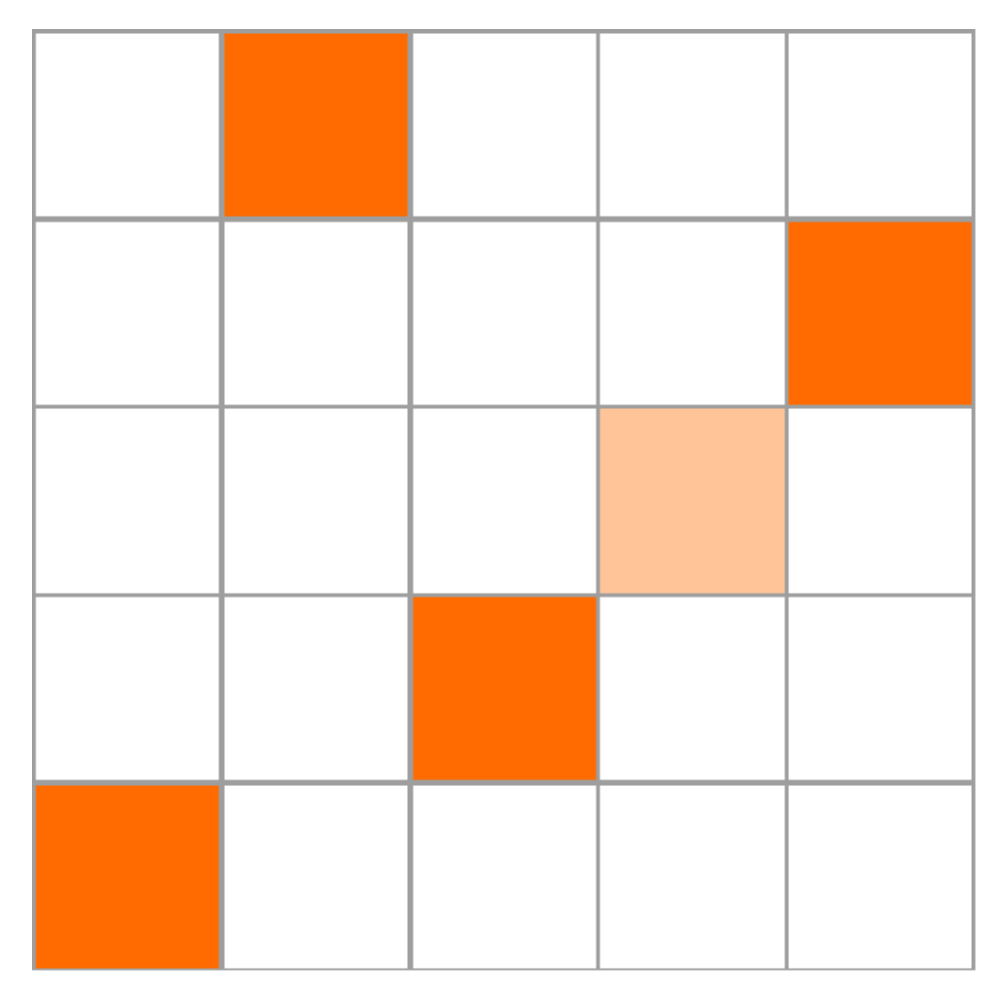Geometrically, if the measure $\mu$ is plotted as a discrete heat map in the j-discrete unit square, then no color element in the plot has another color element in its same row and column, as can be seen in Figure 2.

Definition 1. 

We define a proximity criteria in the j-discrete unit square as follows: $(i,k)$ is a neighbor of $(l,m)$ if

$$|i-l|=1\mathrm{or}|k-m|=1.$$

(41)

In Figure 2, we plot the support of the hypothetical simple solution $\mu$. Hence, the neighbors of the position in the middle of the cross are those that touch the yellow stripes. Then in this example, the middle point has four neighbors.

Figure 2. Support of $\mu$ and the proximity criteria.

Figure 2. Support of $\mu$ and the proximity criteria.

With this in mind, we can classify the points in $support(\mu )$ as follows.

Definition 2. 

We say that $(k_1,k_2)\in support(\mu )$ is a border point if $k_1$ or $k_2$ equals 0 or 1; otherwise, we call it an interior point. It is clear that a border point has at least one neighbor and at most three, whereas an interior point has at least two neighbors and at most four. Hence, we can partition $support(\mu )$ into two sets as follows.

The set of the points of Type I is given by

$$T_1=\{(i,k)\in support(\mu )|(i,k)\mathit{has}\mathit{minimun}\mathit{neighbors}\},$$

(42)

and the set of the points of Type II is given by

$$T_2=support(\mu )\backslash T_1.$$

(43)

Intuitively, the set $T_1$ is composed of well-controlled points, whereas the set $T_2$ has the points that admit permutations between them, since, as we will see in the next section, in the proposed algorithm they will be permuted. See Figure 3 and Figure 4. Naturally, since $\mu$ is a feasible solution for (40), then given elements $(k_1,k_2),(m_1,m_2)\in support(\mu )$ and for $i=1,2$ permutations ${\sigma }_i$ over $\{k_i,m_i\}$, the measure ${\mu }^{\sigma }$ defined by

$${\mu }^{\sigma }(a,b)=\mu ({\sigma }_1(a),{\sigma }_2(b))$$

(44)

is a feasible solution.

Figure 3. Classification of the points in $support(\mu )$: Type I points.

Figure 3. Classification of the points in $support(\mu )$: Type I points.

Figure 4. Classification of the points in $support(\mu )$: Type II points.

Figure 4. Classification of the points in $support(\mu )$: Type II points.

Refining Projections

In this subsection, we study the problem of improving an optimal solution ${\mu }_{j-1}^{*}$ for (40) on level $j-1\in \mathbb{Z}$ to a feasible solution ${\widehat{\mu }}_j$ for the next level j. Let ${\mu }_{j-1}^{*}$ be an optimal solution for level $j-1$. Then we are looking for ${\widehat{\mu }}_j$ such that:

$$\begin{array}{cc}\hfill (1)& {\widehat{\mu }}_j\mathrm{is}\mathrm{a}\mathrm{feasible}\mathrm{solution}.\hfill \\ \hfill (2)& {\mathbf{P}}_{j-1}{\widehat{\mu }}_j={\mu }_{j-1}^{*}.\hfill \end{array}$$

(45)

As described in the previous section, the measure ${\widehat{\mu }}_j\in L^2({\mathbb{R}}^2)$ can be decomposed in

$${\widehat{\mu }}_j={\mu }_{j-1}^{*}+{\nu }_1+{\nu }_2+{\nu }_3$$

(46)

where

$$\begin{array}{cc}\hfill {\nu }_i(x,y)& =({\mathbf{Q}}_j^{(i)}{\widehat{\mu }}_j)(x,y)\hfill \\ \hfill & =\sum _{k_1}\sum _{k_2}\langle {\widehat{\mu }}_j,{\Psi }_{j,k_1,k_2}^{(i)}\rangle {\Psi }_{j,k_1,k_2}^{(i)}(x,y).\hfill \end{array}$$

(47)

From the geometric point of view, the projections ${\nu }_i$ are formed from differences of characteristic functions, as we mentioned in Section 2.2. So we have the following result:

Lemma 1. 

Let $j\in \mathbb{Z}$ and ${\mu }_{j-1}^{*}$ be an optimal solution for (40) at level $j-1$. Then for each positive measure ${\widehat{\mu }}_j\in {\mathbf{P}}_j{L}^2({\mathbb{R}}^2)$ such that ${\mathbf{P}}_{j-1}{\widehat{\mu }}_j={\mu }_{j-1}^{*}$ and ${\widehat{\mu }}_j={\mu }_{j-1}^{*}+{\nu }_1+{\nu }_2+{\nu }_3$, it necessarily holds that

$${\mu }_{j-1}^{*}(A)=0\mathit{implies}{\nu }_i(A)=0$$

(48)

for each Lebesgue measurable set $A\subset {\mathbb{R}}^2$ and each $i=1,2,3$. Therefore, the support of ${\widehat{\mu }}_j$ is contained in the support of ${\mu }_{j-1}^{*}$.

Proof. 

We only make the proof for the case $i=1$, since the other two are very similar. To simplify the notation, we use the symbols ${\mu }_{-}$ and ${\nu }_{-}$ as measures or functions in the respective subspace of $L^2({\mathbb{R}}^2)$. Since when setting a level $j\in \mathbb{Z}$ all the measures in question are constant in pairs of rectangles dividing $S(j,k_1,k_2)$, as we prove in Section 2.2, then it is enough to prove that (65) is valid on this rectangles. Let

$$\begin{array}{cc}\hfill A_1& =A_1(j,k_1^{\prime },k_2^{\prime })\hfill \\ \hfill & =[2^{-j}{k}_1^{\prime },2^{-j}(k_1^{\prime }+1))\times [2^{-j-1}2k_2^{\prime },2^{-j-1}(2k_2^{\prime }+1)).\hfill \end{array}$$

(49)

and

$$\begin{array}{cc}\hfill A_2& =A_2(j,k_1^{\prime },k_2^{\prime })\hfill \\ \hfill & =[2^{-j}{k}_1^{\prime },2^{-j}(k_1^{\prime }+1))\times [2^{-j-1}2k_2^{\prime }+1,2^{-j-1}(2k_2^{\prime }+2)),\hfill \end{array}$$

(50)

as in (22). Then for $l=1,2$, we have that

$$\begin{array}{cc}\hfill {\widehat{\mu }}_j(A_l)& {\displaystyle ={\mu }_{j-1}^{*}(A_l)+\sum _{i=1}^3{\nu }_i(A_l)}\hfill \\ \hfill & {\displaystyle =\mathbb{E}[{\mu }_{j-1}^{*}{\chi }_{A_l}]+\sum _{i=1}^3\mathbb{E}[{\nu }_i{\chi }_{A_l}].}\hfill \end{array}$$

(51)

Now we will calculate each one of the expectations separately. By (17), (18) and (25), we have that

$$\begin{array}{cc}\hfill {\mu }_{j-1}^{*}(x,y)& =\sum _{k_1}\sum _{k_2}\langle {\mu }_{j-1}^{*},{\Phi }_{j,k_1,k_2}\rangle {\Phi }_{j,k_1,k_2}(x,y)\hfill \end{array}$$

(52)

and

$$\begin{array}{cc}\hfill {\nu }_1(x,y)& =\sum _{k_1}\sum _{k_2}\langle {\nu }_1,{\Psi }_{j,k_1,k_2}^{(1)}\rangle {\Psi }_{j,k_1,k_2}^{(1)}(x,y)\hfill \\ \hfill & =\sum _{k_1}\sum _{k_2}\langle {\nu }_1,{\Psi }_{j,k_1,k_2}^{(1)}\rangle [{\chi }_{A_1(j,k_1,k_2)}(x,y)-{\chi }_{A_2(j,k_1,k_2)}(x,y)].\hfill \end{array}$$

(53)

Then for $l=1$ and by (15), (16) and (22), we have that

$$\begin{array}{cc}\hfill \mathbb{E}[{\mu }_{j-1}^{*}{\chi }_{A_1}]& =\mathbb{E}[{\chi }_{A_1}\sum _{k_1}\sum _{k_2}\langle {\mu }_{j-1}^{*},{\Phi }_{j,k_1,k_2}\rangle {\Phi }_{j,k_1,k_2}]\hfill \\ \hfill & =\langle {\mu }_{j-1}^{*},{\Phi }_{j,k_1^{\prime },k_2^{\prime }}\rangle \mathbb{E}[{\chi }_{A_1}{\Phi }_{j,k_1^{\prime },k_2^{\prime }}]]\hfill \\ \hfill & =d\mathbb{E}[{\chi }_{A_1}]\hfill \\ \hfill & {\displaystyle =d\frac{1}{2^{2j+1}}}\hfill \end{array}$$

(54)

where $d=\langle {\mu }_{j-1}^{*},{\Phi }_{j,k_1^{\prime },k_2^{\prime }}\rangle$ and

$$\begin{array}{cc}\hfill \mathbb{E}[{\nu }_1{\chi }_{A_1}]& =\mathbb{E}[{\chi }_{A_1}\sum _{k_1}\sum _{k_2}\langle {\nu }_1,{\Psi }_{j,k_1,k_2}^{(1)}\rangle ({\chi }_{A_1(j,k_1,k_2)}-{\chi }_{A_2(j,k_1,k_2)})]\hfill \\ \hfill & =\langle {\nu }_1,{\Psi }_{j,k_1^{\prime },k_2^{\prime }}^{(1)}\rangle \mathbb{E}{\chi }_{A_1}\hfill \\ \hfill & =c\mathbb{E}[{\chi }_{A_1}]\hfill \\ \hfill & {\displaystyle =c\frac{1}{2^{2j+1}}}\hfill \end{array}$$

(55)

where $c=\langle {\nu }_1,{\Psi }_{j,k_1^{\prime },k_2^{\prime }}^{(1)}\rangle$. Similarly, but using (23) and (24), we can prove that

$$\mathbb{E}[{\nu }_2{\chi }_{A_1}]=0$$

(56)

and

$$\mathbb{E}[{\nu }_3{\chi }_{A_1}]=0.$$

(57)

Then

$$\begin{array}{cc}\hfill {\widehat{\mu }}_j(A_1)& {\displaystyle =d\frac{1}{2^{2j+1}}+c\frac{1}{2^{2j+1}}}\hfill \\ \hfill & ={\mu }_{j-1}^{*}(A_1)+\nu (A_1)\hfill \end{array}$$

(58)

Now, we will make an analogous argument for the case $l=2$. Hence,

$$\begin{array}{cc}\hfill \mathbb{E}[{\mu }_{j-1}^{*}{\chi }_{A_2}]& =\mathbb{E}[{\chi }_{A_2}\sum _{k_1}\sum _{k_2}\langle {\mu }_{j-1}^{*},{\Phi }_{j,k_1,k_2}\rangle {\Phi }_{j,k_1,k_2}]\hfill \\ \hfill & =\langle {\mu }_{j-1}^{*},{\Phi }_{j,k_1,k_2}\rangle \mathbb{E}[{\chi }_{A_2}{\Phi }_{j,k_1^{\prime },k_2^{\prime }}]]\hfill \\ \hfill & =d\mathbb{E}[{\chi }_{A_2}]\hfill \\ \hfill & {\displaystyle =d\frac{1}{2^{2j+1}}}\hfill \end{array}$$

(59)

and

$$\begin{array}{cc}\hfill \mathbb{E}[{\nu }_1{\chi }_{A_2}]& =\mathbb{E}[{\chi }_{A_2}\sum _{k_1}\sum _{k_2}\langle {\nu }_1,{\Psi }_{j,k_1,k_2}^{(1)}\rangle ({\chi }_{A_1(j,k_1,k_2)}-{\chi }_{A_2(j,k_1,k_2)})]\hfill \\ \hfill & =-\langle {\nu }_1,{\Psi }_{j,k_1^{\prime },k_2^{\prime }}^{(1)}\rangle \mathbb{E}{\chi }_{A_2}\hfill \\ \hfill & =-c\mathbb{E}[{\chi }_{A_2}]\hfill \\ \hfill & {\displaystyle =-c\frac{1}{2^{2j+1}}.}\hfill \end{array}$$

(60)

Thus,

$$\begin{array}{cc}\hfill {\widehat{\mu }}_j(A_2)& {\displaystyle =d\frac{1}{2^{2j+1}}-c\frac{1}{2^{2j+1}}}\hfill \\ \hfill & ={\mu }_{j-1}^{*}(A_2)+\nu (A_2)\hfill \end{array}$$

(61)

and by (54), (55), (59) and (60), we have that

$${\mu }_{j-1}^{*}(A_1)={\mu }_{j-1}^{*}(A_2)$$

(62)

and

$${\nu }_1(A_1)=-{\nu }_1(A_2).$$

(63)

Therefore, it follows from (58), (61), (62), (63) and the fact that ${\widehat{\mu }}_j$ is a positive measure, that

$$\begin{array}{cc}\hfill |{\nu }_1(A_1)|& =|{\nu }_1(A_2)|\hfill \\ \hfill & \le |{\mu }_{j-1}^{*}(A_1)|\hfill \\ \hfill & =|{\mu }_{j-1}^{*}(A_2)|\hfill \end{array}$$

(64)

From which we conclude that ${\mu }_{j-1}^{*}(A)=0$ implies ${\nu }_1(A)=0$. Similarly, it can be shown that ${\mu }_{j-1}^{*}(A)=0$ implies ${\nu }_i(A)=0$ for $i=2,3$; for this, analogous proofs are carried out, with the difference being that for $i=2$, the sets to be considered are $B_1$ and $B_2$ as in (23), whereas $C_1\cup C_4$ and $C_2\cup C_3$ as in (24) are the respective sets when $i=3$. □

We have proved that if it is intended to go back to the preimage of the projection of the approximation operator $\mathbf{P}$ from a level $j-1$ to a level j, the support of the level $j-1$ delimits that of the j level. Now, we will prove that for every measure ${\widehat{\mu }}_j$ that satisfies (45) and (46), it necessarily holds that ${\nu }_1={\nu }_2=0$.

Lemma 2. 

Let $j\in \mathbb{Z}$ and ${\mu }_{j-1}^{*}$ be an optimal simple solution for (40) at level $j-1$. Then for each feasible solution ${\widehat{\mu }}_j\in {\mathbf{P}}_j{L}^2({\mathbb{R}}^2)$ to (40) at level j such that ${\mathbf{P}}_{j-1}{\widehat{\mu }}_j={\mu }_{j-1}^{*}$ and ${\widehat{\mu }}_j={\mu }_{j-1}^{*}+{\nu }_1+{\nu }_2+{\nu }_3$. It necessarily holds that

$${\nu }_1={\nu }_2=0.$$

(65)

Proof. 

In order to perform this proof, we use the restrictions of the $\mathrm{MK}$ problem (40), which in turn, are related to the marginal measures. Therefore, we will only complete the proof for one of the projections, since the other is analogous. From the linearity of the Radon–Nikodym derivative, it follows that

$$\begin{array}{cc}\hfill {\eta }_j^1& ={\Pi }_1{\widehat{\mu }}_j\hfill \\ \hfill & =\Pi ({\mu }_{j-1}^{*}+{\nu }_1+{\nu }_2+{\nu }_3)\hfill \\ \hfill & =\Pi {\mu }_{j-1}^{*}+\Pi {\nu }_1+\Pi {\nu }_2+\Pi {\nu }_3.\hfill \end{array}$$

(66)

Let $k^{\prime }\in \mathbb{Z}$ and $I_{j+1,2k^{\prime }}=[2^{-j-1}2k^{\prime },2^{-j-1}(2k^{\prime }+1))$. Thus, by (39) and (66), we have that

$$\begin{array}{cc}\hfill {\Pi }_1{\widehat{\mu }}_j(I_{j+1,2k^{\prime }})& ={\eta }_j^1(I_{j+1,2k^{\prime }})\hfill \\ \hfill & ={\Pi }_1{\mu }_{j-1}^{*}(I_{j+1,2k^{\prime }})\hfill \\ \hfill & =\alpha .\hfill \end{array}$$

(67)

That is, we are evaluating feasible solutions on rectangles whose height is half the size of the squares with which they are discretized at the j level of the Haar MRA. Now, we will develop in detail (66) evaluated on $I_{j,k^{\prime }}$. Since ${\mu }_{j-1}^{*}$ is a simple solution, we call $l^{\prime }\in \mathbb{Z}$ the only number such that ${\mu }_{j-1}^{+}(S(j,k^{\prime },l^{\prime }))>0$, where $S(j,k_1,k_2)$ is defined as in (20). With the aim of simplifying the notation, we define $\mathcal{I}=I_{j+1,2k^{\prime }}\times \mathbb{R}$. By (16) and (25), we have that

$$\begin{array}{cc}\hfill {\Pi }_1{\nu }_1(I_{j+1,2k^{\prime }})& ={\nu }_i(\mathcal{I})\hfill \\ \hfill & =\mathbb{E}[{\chi }_{\mathcal{I}}{\nu }_1]\hfill \\ \hfill & =\mathbb{E}[{\chi }_{\mathcal{I}}\sum _{k_1}\sum _{k_2}\langle {\nu }_1,{\Psi }_{j,k_1,k_2}^{(1)}\rangle ({\chi }_{A_1(j,k_1,k_2)}-{\chi }_{A_2(j,k_1,k_2)})]\hfill \\ \hfill & =\mathbb{E}[{\chi }_{\mathcal{I}}\sum _{k_2}\langle {\nu }_1,{\Psi }_{j,k^{\prime },k_2}^{(1)}\rangle ({\chi }_{A_1(j,k^{\prime },k_2)}-{\chi }_{A_2(j,k^{\prime },k_2)})]\hfill \\ \hfill & =\mathbb{E}[{\chi }_{\mathcal{I}}\langle {\nu }_1,{\Psi }_{j,k^{\prime },l^{\prime }}^{(1)}\rangle ({\chi }_{A_1(j,k^{\prime },l^{\prime })}-{\chi }_{A_2(j,k^{\prime },l^{\prime })})]\hfill \end{array}$$

(68)

By the way $\mathcal{I}$ was defined, necessarily in the last equality it must be fulfilled that one of the terms in the expectation is equal to 0. Hence, it is fulfilled that

$$\begin{array}{cc}\hfill {\Pi }_1{\nu }_1(I_{j+1,2k^{\prime }})& =\langle {\nu }_1,{\Psi }_{j,k^{\prime },l^{\prime }}^{(1)}\rangle \mathbb{E}[{\chi }_{\mathcal{I}}]\hfill \\ \hfill & {\displaystyle =\frac{1}{2^{2j+1}}\langle {\nu }_1,{\Psi }_{j,k^{\prime },l^{\prime }}^{(1)}\rangle .}\hfill \end{array}$$

(69)

By a similar argument, it can be proved that

$$\Pi {\nu }_2(I_{j+1,2k^{\prime }})=0$$

(70)

and

$$\Pi {\nu }_2(I_{j+1,2k^{\prime }})=0.$$

(71)

Then from (66) to (71), it follows that

$${\displaystyle \alpha =\alpha +\frac{1}{2^{2j+1}}\langle {\nu }_1,{\Psi }_{j,k^{\prime },l^{\prime }}^{(1)}\rangle +0+0.}$$

(72)

Hence,

$$\langle {\nu }_1,{\Psi }_{j,k^{\prime },l^{\prime }}^{(1)}\rangle =0.$$

(73)

Therefore, ${\nu }_1=0$. In a similar way, we can prove that ${\nu }_2=0$. □

Suppose we have a simple optimal solution ${\mu }_{j-1}^{*}$ for the $\mathrm{MK}$ problem discretized through the Haar MRA at level $j-1\in \mathbb{Z}$ and that we are interested in refining that solution to the next level j. By Lemmas 1 and 2, any ${\widehat{\mu }}_j$ that satisfies (45) has its support contained in the support of ${\mu }_{j-1}^{*}$ and has components ${\nu }_1={\nu }_2=0$. Then the problem of constructing a feasible solution ${\widehat{\mu }}_j$ such that it refines ${\mu }_{j-1}^{*}$ is reduced to construct

$$\begin{array}{cc}\hfill {\widehat{\mu }}_j(x,y)& ={\mu }_{j-1}^{*}(x,y)+{\nu }_3(x,y)\hfill \\ \hfill & ={\mu }_{j-1}^{*}(x,y)+\sum _{k_1}\sum _{k_2}\langle {\widehat{\mu }}_j,{\Psi }_{j,k_1,k_2}^{(i)}\rangle {\Psi }_{j,k_1,k_2}^{(i)}(x,y),\hfill \end{array}$$

(74)

which is equivalent to chosing for each $k_1,k_2\in \mathbb{Z}$ a value ${\nu }_{k_1,k_2}^3$ such that

$${\widehat{\mu }}_{k_1,k_2}^j={\mu }_{k_1,k_2}^{*,j-1}+{\nu }_{k_1,k_2}^3.$$

(75)

By Lemma 1 for each $k_1,k_2\in \mathbb{Z}$, it is fulfilled that

$$|{\nu }_{k_1,k_2}^3|\le {\mu }_{k_1,k_2}^{*,j-1}.$$

(76)

Therefore, the choice of ${\nu }_{k_1,k_2}^3$ is restricted to a compact collection, and since ${\widehat{\mu }}_j$ is a solution of the linear program (40), then

$$|{\nu }_{k_1,k_2}^3|={\mu }_{k_1,k_2}^{*,j-1}.$$

(77)

Thus, the sign of ${\nu }_{k_1,k_2}^3$ must be such that it minimizes ${\nu }_{k_1,k_2}^3{c}_{k_1,k_2}^j$. That is,

$${\nu }_{k_1,k_2}^3{c}_{k_1,k_2}^j\le 0$$

(78)

4. Methodological Proposal

In this section, we show through examples a process that builds solutions to the $\mathrm{MK}$ problem with a reduced number of operations. First, we consider the $\mathrm{MK}$ problem with cost function $c:[0,1]\times [0,1]\to \mathbb{R}$ defined by

$$c(x,y)=4x^{2}y-x{y}^2$$

(79)

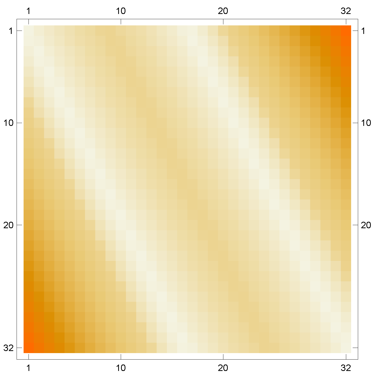
and homogeneous restrictions ${\nu }_1,{\nu }_2$ over $[0,1]$. So that the algorithm can be graphically appreciated, we take a small level of discretization, namely $j=6$. Thus, in the Haar MRA over ${\mathbb{R}}^2$ at level $j=6$, the cost function has the form shown in Figure 5, which can be stored in a vector of size $2^{2j}=2^{2(6)}=2^{12}$.

Now, we apply the filtering process to the cost function at level $j=6$, which results in four functions

$$c_6(x,y)=c_5(x,y)+{\Psi }^{(1)}(x,y)+{\Psi }^{(2)}(x,y)+{\Psi }^{(3)}(x,y);$$

(80)

see Figure 6, Figure 7, Figure 8 and Figure 9.

Figure 5. Step 1. Discretization of the cost function to the level j, which is denoted by $c_j$. In particular, the cost function is $c(x,y)=4x^{2}y-x{y}^2$ for lever $j=6$.

Figure 5. Step 1. Discretization of the cost function to the level j, which is denoted by $c_j$. In particular, the cost function is $c(x,y)=4x^{2}y-x{y}^2$ for lever $j=6$.

Step 2. Filtering the original discrete function using the high-pass filter, which yield three discrete functions denoted by ${\Psi }_1$, ${\Psi }_2$ and ${\Psi }_3$, that functions correspond to Figure 7, Figure 8 and Figure 9, respectively, each describing local changes in the original discrete function. It is then low-pass filtered to produce the approximate discrete function $c_5$, which is given by Figure 6.

Figure 6. $c_5(x,y)$.

Figure 6. $c_5(x,y)$.

Figure 7. ${\Psi }^{(1)}(x,y)$.

Figure 7. ${\Psi }^{(1)}(x,y)$.

Figure 8. ${\Psi }^{(2)}(x,y)$.

Figure 8. ${\Psi }^{(2)}(x,y)$.

Figure 9. ${\Psi }^{(3)}(x,y)$.

Figure 9. ${\Psi }^{(3)}(x,y)$.

We then solve the $\mathrm{MK}$ problem for the level $j-1=5$. That is, we find a measure ${\mu }_{j-1}^{*}={\mu }_5^{*}$ that is an optimal solution for the $\mathrm{MK}$ problem with cost function $c_5$. Such data can be stored in a vector of size $2^{2j-2}=2^{10}$; see Figure 10. For each entry k, the formal application that plots this vector in a square is defined by $k\to (k_1+1,k_2+1)$, where $0\le k_1,k_2<2^{n-1}$ and $k=k_1·2^{j-1}+k_2$.

Since the measure ${\mu }_{j-1}^{*}={\mu }_5^{*}$ is an optimal simple solution for the $\mathrm{MK}$ problem, then we can represent its support in a simple way, as we show below:

$${\displaystyle support({\mu }_{j-1}^{*})=\bigcup _{k_1,k_2}{S}_{k_1,k_2}}$$

(81)

where $S_{k_1,k_2}=S(j,k_1,k_2)$ is the square in (20). Next, we split each block $S_{k_1,k_2}\subset support({\mu }_{j-1}^{*})$ into four parts as in (24); see Figure 11.

From the technical point of view, in the discretization at level $j-1=5$, we have a grid of $2^{j-1}\times 2^{j-1}=32\times 32$ squares that we call $S_{k_1,k_2}$ and identify with the points $(k_1,k_2)$. Thus, we refine to a grid of $64\times 64$, splitting each square into four, which in the new grid are determined by points

$$(2k_1-1,2k_2),(2k_1-1,2k_2-1),(2k_1,2k_2-1)\mathrm{and}(2k_1,2k_2);$$

(82)

see Figure 12.

As we prove in Lemma 1, any feasible solution ${\widehat{\mu }}_j={\widehat{\mu }}_6$ that refines ${\mu }_5^{*}$ has its support contained in $support({\mu }_5^{*})$. Therefore, we must only deal with the region delimited by the support of ${\mu }_5^{*}$. By Lemma 2, in order to construct the solution ${\widehat{\mu }}_6$, we only need to determine the values $n_{k_1,k_2}^3$ corresponding to the coefficients of the wavelet part ${\nu }_3$; however, by (77) and (78), those values are well determined and satisfy that when added with the scaling part ${\mu }_{k_1,k_2}^{*}$, the result is a scalar multiple of a characteristic function. For example if the square $S_{k_1,k_2}$ has scaling part coefficient ${\mu }_{k_1,k_2}^{*}=c$, then we choose ${\nu }_{k_1,k_2}^3=-c$. Hence, by (21) and (25), we have that

$$\begin{array}{cc}\hfill {\widehat{\mu }}_{k_1,k_2}^6(x,y)& ={\mu }_{k_1,k_2}^{*}(x,y)+{\nu }_{k_1,k_2}^3(x,y)\hfill \\ \hfill & {\displaystyle =c{\chi }_S(x,y)-c[{\chi }_{C_1\cup C_4}(x,y)-{\chi }_{C_2\cup C_3}(x,y)]}\hfill \\ \hfill & =2c{\chi }_{C_2\cup C_3}(x,y).\hfill \end{array}$$

(83)

Thus, from an operational point of view, we only need to chose between two options of supporting each division of square $S_{k_1,k_2}$, as we illustrate in Figure 13 and Figure 14.

This coincides with our geometric intuition. Hence, the resulting feasible solution ${\widehat{\mu }}_6$ has its support contained in $support({\mu }_5^{*})$, and its weight within each square $S_{k_1,k_2}$ is presented in a diagonal within that block; see Figure 15. Finally, we can improve ${\widehat{\mu }}_6$ by observing the way the filtering process acts. To do this, we apply the proximity criteria (41) and split the support of ${\widehat{\mu }}_6$ into points of Type I and II. In Figure 16, we identify the points of Type I and II of solution ${\mu }_5^{*}$, whereas in Figure 15, we do the same but for ${\widehat{\mu }}_6$.

Intuitively, the division of the support into points of Type I and II allows us to classify the points so that they have an identity function form and, consequently, that come from the discretization of a continuous function—points of Type I—and in points that come from the discretization of a discontinuous function—points of Type II. Thus, the points of Type I are located in such a way that they generate a desired solution, and therefore it is not convenient to move them, whereas Type II points are free to be changed as this does not lead to the destruction of a continuous structure in the solution. As we mentioned in the previous section, each permutation of rows or columns of one weighted element $S_{k_1,k_2}$ with another $S_{k_1^{\prime },k_2^{\prime }}$ constructs a feasible solution; see (44). Thus, as a heuristic technique to improve the solution, we check the values $\langle c_6,{\mu }_6^{\sigma }\rangle$ associated with each solution ${\mu }_6^{\sigma }$ obtained by permuting rows or columns of points of Type II of the solution ${\widehat{\mu }}_6$. We call ${\mu }_6^{{\sigma }^{*}}$ the solution for which its permutation gives it the best performance. See Figure 17.

Figure 15. Step 5. Using the solution ${\mu }_5^{*}$ which is given by Figure 10, the information of the high-pass components (Figure 7, Figure 8 and Figure 9) and Lemma 1, we obtain a feasible solution for Level 6, which is denoted by ${\widehat{\mu }}_6$.

Figure 15. Step 5. Using the solution ${\mu }_5^{*}$ which is given by Figure 10, the information of the high-pass components (Figure 7, Figure 8 and Figure 9) and Lemma 1, we obtain a feasible solution for Level 6, which is denoted by ${\widehat{\mu }}_6$.

Figure 16. Step 4. We classify the points of the support of the solution ${\mu }_5^{*}$ by proximity criteria as points of Type I ■ or Type II ■ (the measure ${\mu }_5^{*}$ corresponds to Figure 10).

Figure 16. Step 4. We classify the points of the support of the solution ${\mu }_5^{*}$ by proximity criteria as points of Type I ■ or Type II ■ (the measure ${\mu }_5^{*}$ corresponds to Figure 10).

Finally, we present

Table 1. Comparison of the values corresponding to ${\mathrm{MK}}_5$, ${\mathrm{MK}}_6^{{\sigma }^{*}}$ and ${\mathrm{MK}}_6$.

${\mathbf{MK}}_5$	${\mathbf{MK}}_6^{{\mathit{\sigma }}^{*}}$	${\mathbf{MK}}_6$
$0.24785$	$0.247738$	$0.247726$

that compare the solutions of the $\mathrm{MK}$ problem, in which ${\mathrm{MK}}^5$ is the value associated with the optimal solution ${\mu }_5^{*}$ at level of discretization $j-1=5$, ${\mathrm{MK}}_6$ is the value associated with an optimal solution ${\mu }_6^{*}$ at level of discretization $j=6$, and ${\mathrm{MK}}_6^{{\sigma }^{*}}$ is the value associated with the solution ${\mu }_6^{{\sigma }^{*}}$ obtained by the heuristic method described in the previous paragraph.

Figure 17. Step 6. Classification of the points of ${\mu }_5^{*}$ induces classification of the points in ${\widehat{\mu }}_6$ by contention in the support. Over the points of Type I of the solution ${\widehat{\mu }}_6$, we do not move those points. For the points of Type II, we apply a permutation to the solution over the two points that improve the solution and repeat the process with the rest of the points.

Figure 17. Step 6. Classification of the points of ${\mu }_5^{*}$ induces classification of the points in ${\widehat{\mu }}_6$ by contention in the support. Over the points of Type I of the solution ${\widehat{\mu }}_6$, we do not move those points. For the points of Type II, we apply a permutation to the solution over the two points that improve the solution and repeat the process with the rest of the points.

5. Other Examples of This Methodology

We conclude this work with a series of examples in which we apply the proposed methodology. Each of them is divided into the six-step algorithm introduced in the previous section and corresponds to a classical example existing in the literature.

5.1. Example with Cost Function $c(x,y)=x^{2}y-x{y}^2$

Let $\mathrm{MK}$ be the $\mathrm{MK}$ problem with cost function $c(x,y)=x^{2}y-x{y}^2$ and uniform restrictions ${\eta }_1$ and ${\eta }_2$ over the unitary interval $[0,1]$. In order to be more didactic, we consider the level of discretization $j=6$. Next, we present the reduced algorithm.

Step 1.

Discretize the cost function at level j—that is, over a grid of $2^j\times 2^j$. Figure 18.

Step 2.

Apply the filtering process to the cost function at level $j-1$, obtaining the filtered cost function $c_5$, which is plotted on a grid of $2^{j-1}\times 2^{j-1}$. Figure 19.

Step 3.

Find an optimal simple solution ${\mu }_{j-1}^{*}$ for the discretized $M{K}_j$ problem. That is, solve for the cost function $c_5$ and obtain an optimal simple solution ${\mu }_5^{*}$. Figure 20.

Step 4.

Apply the proximity criteria to the support of ${\mu }_{j-1}^{*}$. Figure 21.

Step 5.

Refine the optimal simple solution ${\mu }_{j-1}^{*}$ to a feasible solution ${\widehat{\mu }}_j$, dividing each weighted square $S_{k_1,k_2}$ at level $j-1$ into four squares at level j (see (82)) and place mass according to the criteria (83). Figure 22.

Step 6.

Permute the rows and columns of the points of Type II in $support({\widehat{\mu }}_j)$ using (44) to construct feasible solutions ${\mu }_j^{\sigma }$ and chose the one that has better performance. Figure 23.

The following

Table 2. Comparison of the values corresponding to ${\mathrm{MK}}_5$, ${\mathrm{MK}}_6^{{\sigma }^{*}}$ and ${\mathrm{MK}}_6$.

${\mathbf{MK}}_5$	${\mathbf{MK}}_6^{{\mathit{\sigma }}^{*}}$	${\mathbf{MK}}_6$
$-0.0350952$	$-0.035141$	$-0.035141$

contains the comparison of the proposed methodology with the two immediate levels of resolution.

5.2. Example with Cost Function $c(x,y)=xy$

Let $\mathrm{MK}$ be the $\mathrm{MK}$ problem with cost function $c(x,y)=xy$ and uniform restrictions ${\eta }_1$ and ${\eta }_2$ over the unitary interval $[0,1]$. In order to be more didactic, we consider the level of discretization $j=6$. Next, we present the reduced algorithm.

Step 1.

Discretize the cost function at level j—that is, over a grid of $2^j\times 2^j$. Figure 24.

Step 2.

Apply the filtering process to the cost function at level $j-1$, obtaining the filtered cost function $c_5$, which is plotted on a grid of $2^{j-1}\times 2^{j-1}$. Figure 25.

Step 3.

Find an optimal simple solution ${\mu }_{j-1}^{*}$ for the discretized $M{K}_j$ problem. That is, solve for the cost function $c_5$ and obtain an optimal simple solution ${\mu }_5^{*}$. Figure 26.

Step 4.

Apply the proximity criteria to the support of ${\mu }_{j-1}^{*}$. Figure 27.

Step 5.

Refine the optimal simple solution ${\mu }_{j-1}^{*}$ to a feasible solution ${\widehat{\mu }}_j$, dividing each weighted square $S_{k_1,k_2}$ at level $j-1$ into four squares at level j (see (82)) and placing mass according to the criteria (83). Figure 28.

Step 6.

Permute the rows and columns of the points of Type II in $support({\widehat{\mu }}_j)$ using (44) to construct feasible solutions ${\mu }_j^{\sigma }$ and chose the one that has better performance. Figure 29.

The following

Table 3. Comparison of the values corresponding to ${\mathrm{MK}}_5$, ${\mathrm{MK}}_6^{{\sigma }^{*}}$ and ${\mathrm{MK}}_6$.

${\mathbf{MK}}_5$	${\mathbf{MK}}_6^{{\mathit{\sigma }}^{*}}$	${\mathbf{MK}}_6$
$0.166748$	$0.166687$	$0.166687$

contains the comparison of the proposed methodology with the two immediate levels of resolution.

5.3. Example with Cost Function $c(x,y)={(2y-x-1)}^2{(2y-x)}^2$

We take the $\mathrm{MK}$ problem with cost function $c(x,y)={(2y-x-1)}^2{(2y-x)}^2$ and homogeneous restrictions over the unitary interval. Again, we consider the level of discretization $j=6$.

Step 1.

Discretize the cost function at level j. Figure 30.

Step 2.

Apply the filtering process at level $j-1$ to the cost function. Figure 31.

Step 3.

Find an optimal simple solution ${\mu }_{j-1}^{*}$ for the ${\mathrm{MK}}_{j-1}$ problem. Figure 32.

Step 4.

Apply the proximity criteria to the support of ${\mu }_{j-1}^{*}$. Figure 33.

Step 5.

Refine the solution ${\mu }_{j-1}^{*}$ to a feasible solution ${\widehat{\mu }}_6$ applying the criteria (82) and (83). Figure 34.

Step 6.

Permute points of Type II of ${\widehat{\mu }}_j$ using (44) to construct feasible solutions ${\mu }_j^{\sigma }$ and chose which has better performance. Figure 35.

The

Table 4. Comparison of values ${\mathrm{MK}}_5$, ${\mathrm{MK}}_6^{{\sigma }^{*}}$ and ${\mathrm{MK}}_6$.

${\mathbf{MK}}_5$	${\mathbf{MK}}_6^{{\mathit{\sigma }}^{*}}$	${\mathbf{MK}}_6$
$0.000236571$	$0.0000600852$	$0.0000597889$

summarizes the results obtained.

6. Conclusions and Future Work

Note that with the methodology of [3,4,9], the authors obtain a solution of $M{K}^j$. For this, they need to resolve a transport problem with $4^j$ variables. We call this methodology an exhaustive method. For our methodology, in Step 3, we need to resolve a transport problem with $4^{j-1}$ variables, and the other steps of the methodology are methods of classification, ordering and filtering; with $2^j$ data for classification and ordering and $4^j$ data for filtering, it is clear that this method requires fewer operations to resolve transport problems.

In summary, we have the following table comparing the results of solving the examples more often used in the literature with our methodology versus the exhaustive method (using all variables).

Cost Function	${\mathbf{MK}}^{\mathbf{6}}$	${\mathbf{MK}}_{\mathbf{6}}^{\mathbf{\sigma }}$	Error
$xy$	$0.166687$	$0.166687$
$x^{2}y-x{y}^2$	$-0.035141$	$-0.035141$	$1.52588\times {10}^{-5}$
$4x^{2}y-x{y}^2$	$0.247726$	$0.247738$	$5.31762\times {10}^{-5}$
${(2y-x-1)}^2{(2y-x)}^2$	$0.0000600947$	$0.0000600947$
Cost Function	${\mathbf{MK}}^{\mathbf{7}}$	${\mathbf{MK}}_{\mathbf{7}}^{\mathbf{\sigma }}$	Error
$xy$	$0.166672$	$0.166672$
$x^{2}y-x{y}^2$	$-0.0351524$	$-0.0351524$	$3.8147\times {10}^{-6}$
$4x^{2}y-x{y}^2$	$0.247695$	$0.247698$	$1.24066\times {10}^{-5}$
${(2y-x-1)}^2{(2y-x)}^2$	$0.0000600852$	$0.0000600852$
Cost Function	${\mathbf{MK}}^{\mathbf{8}}$	${\mathbf{MK}}_{\mathbf{8}}^{\mathbf{\sigma }}$	Error
$xy$	$0.166668$	$0.166668$
$x^{2}y-x{y}^2$	$-0.0351553$	$-0.0351553$	$9.53674\times {10}^{-7}$
$4x^{2}y-x{y}^2$	$0.247688$	$0.247688$	$3.21631\times {10}^{-6}$
${(2y-x-1)}^2{(2y-x)}^2$

Note that our method always improves the solution of the level $j-1$ and for some examples give an exact solution; we use Mathematica© and basic computer equipment for programming this methodology, and maybe we can improve the results with software focused on numerical calculus and better computer equipment. It is also important to mention that the methodology presented in this work has some weaknesses. In our computational experiments, we noticed that if we did not start with a sufficient amount of information, then the methodology tended to give very distant results. In other words, if the initial level of discretization was not fine enough, then because the algorithm lowers the resolution level when executed, such loss of information generates poor performance. However, when starting with an adequate level of discretization, experimentally it can be observed that the distribution of the solutions for the discretized problems, as well as the respective optimal values, have stable behavior with a clear trend. The question that arises naturally is: “In practice, what are the parameters that determine good or bad behavior of the algorithm?” Clearly, if the cost function is fixed and we rule out the possible technical problems associated with programming and computing power, the only remaining parameter is the initial refinement level at which the algorithm is going to work—that is, the level j. However, if we reflect more deeply on the reasons why there is a practical threshold beyond which at a certain level of discretization the algorithm has stable behavior, we only have as a possible causes the level of information of the cost function that captures the MR analysis. In other words, if the oscillation of the cost function at a certain level of resolution is well determined by MR analysis, then the algorithm will have good performance.

The approach presented in this paper is far from exhaustive and, on the contrary, opens the possibility for a number of new proposals for approximating solutions to the MK problem. The above is due to the fact that in the work [9], it was proven that discretization of the MK problem can be performed from any MR analysis over ${\mathbb{R}}^2$. Therefore, the possibility of implementing other types of discretions remains open. In principle, as we mentioned in the previous paragraph, the most natural thing is to expect better performance if the nature of the cost function and the types of symmetric geometric structures that it induces in space are studied in order to use an MR analysis that fits this information and therefore has more efficient performance.

References

1. Hernández-Lerma, O.; Lasserre, J.B. Approximation schemes for infinite linear programs. SIAM J. Optim. 1998, 8, 973–988. [Google Scholar] [CrossRef]
2. González-Hernández, J.; Gabriel-Argüelles, J.R.; Hernández-Lerma, O. On solutions to the mass transfer problem. SIAM J. Optim. 2006, 17, 485–499. [Google Scholar] [CrossRef]
3. Gabriel-Argüelles, J.R.; González-Hernández, J.; López-Martínez, R.R. Numerical approximations to the mass transfer problem on compact spaces. IMA J. Numer. Anal. 2010, 30, 1121–1136. [Google Scholar] [CrossRef]
4. Avendaño-Garrido, M.L.; Gabriel-Argüelles, J.R.; Quintana-Torres, L.; Mezura-Montes, E. A metaheuristic for a numerical approximation to the mass transfer problem. Int. J. Appl. Math. Comput. Sci. 2016, 26, 757–766. [Google Scholar] [CrossRef] [Green Version]
5. Avendaño-Garrido, M.L.; Gabriel-Argüelles, J.R.; Quintana-Torres, L.; Mezura-Montes, E. An Efficient Numerical Approximation for the Monge–Kantorovich Mass Transfer Problem. In Machine Learning, Optimization, and Big Data. MOD 2015; Lecture Notes in Computer Science; Pardalos, P., Pavone, M., Farinella, G., Cutello, V., Eds.; Springer: Cham, Switzerland, 2016; Volume 9432, pp. 233–239. [Google Scholar] [CrossRef]
6. Gröchenig, K.; Madych, W.R. Multiresolution analysis, Haar bases, and self-similar tilings of Rn. Inst. Electr. Electron. Eng. Trans. Inf. Theory 1992, 38, 556–568. [Google Scholar] [CrossRef] [Green Version]
7. Liu, Y.; Xu, K.D.; Li, J.; Guo, Y.J.; Zhang, A.; Chen, Q. Millimeter-wave E-plane waveguide bandpass filters based on spoof surface plasmon polaritons. IEEE Trans. Microw. Theory Tech. 2022, 70, 4399–4409. [Google Scholar] [CrossRef]
8. Liu, K.; Yang, Z.; Wei, W.; Gao, B.; Xin, D.; Sun, C.; Gao, G.; Wu, G. Novel detection approach for thermal defects: Study on its feasibility and application to vehicle cables. High Volt. 2023, 8, 358–367. [Google Scholar] [CrossRef]
9. Sánchez-Nungaray, A.; González-Flores, C.; López-Martínez, R.R. Multiresolution Analysis Applied to the Monge–Kantorovich Problem. Abstr. Appl. Anal. 2018, 2018, 1764175. [Google Scholar] [CrossRef]
10. Haker, S.; Tannenbaum, A.; Kikinis, R. Mass Preserving Mappings and Surface Registration; MICCAI 2001, Lecture Notes in Computer Science; Springer: Berlin/Heidelberg, Germany, 2001; Volume 2208, pp. 120–127. [Google Scholar]
11. Zhu, L.; Yang, Y.; Haker, S.; Tannenbaum, A. Optimal mass transport for registration and warping. Int. J. Comput. Vis. 2004, 60, 225–240. [Google Scholar] [CrossRef]
12. Haber, E.; Rehman, T.; Tannenbaum, A. An efficient numerical method for the solution of the L2 optimal mass transfer problem. SIAM J. Sci. Comput. 2010, 32, 7–211. [Google Scholar] [CrossRef] [PubMed] [Green Version]
13. Xie, X.; Wang, T.; Zhang, W. Existence of solutions for the (p, q)-Laplacian equation with nonlocal Choquard reaction. Appl. Math. Lett. 2023, 135, 108418. [Google Scholar] [CrossRef]
14. Peng, Z.; Hu, J.; Shi, K.; Luo, R.; Huang, R.; Ghosh, B.K.; Huang, J. A novel optimal bipartite consensus control scheme for unknown multi-agent systems via model-free reinforcement learning. Appl. Math. Comput. 2020, 369, 124821. [Google Scholar] [CrossRef]
15. Walnut, D.F. An Introduction to Wavelet Analysis; Birkhäuser: Boston, MA, USA, 2004; pp. 115–138. [Google Scholar]
16. Guo, K.; Labate, D.; Lim, W.Q.; Weiss, G.; Wilson, E. Wavelets with composite dilations and their MRA properties. Appl. Comput. Harmon. Anal. 2006, 20, 202–236. [Google Scholar] [CrossRef] [Green Version]
17. Krishtal, I.A.; Robinson, B.D.; Weiss, G.L.; Wilson, E.N. Some simple Haar-type wavelets in higher dimensions. J. Geom. Anal. 2007, 17, 87–96. [Google Scholar] [CrossRef] [Green Version]
18. Bazaraa-Mokhtar, S.; John, J.; Hanif, D. Linear Programming and Network Flows; John Wiley & Sons: Hoboken, NJ, USA, 2010; pp. 513–528. [Google Scholar]
19. Billingsley, P. Convergence of Probability Measures; John Wiley & Sons: New York, NY, USA, 1999; pp. 27–29. [Google Scholar]
Figure 1. Functions Φ j , k 1 , k 2 , Ψ j , k 1 , k 2 ( 1 ) , Ψ j , k 1 , k 2 ( 2 ) and Ψ j , k 1 , k 2 ( 3 ) .
Axioms 12 00555 g001
Figure 10. Step 3. We obtain a solution μ 5 * for M K 5 associated with the cost function c 5 given in Figure 6.
Axioms 12 00555 g010
Figure 11. Division of the components of support ( μ j 1 * ) into four parts.
Axioms 12 00555 g011
Figure 12. Refinement of grid from level j 1 to j of discretization.
Axioms 12 00555 g012
Figure 13. Supports for refinement of the element S k 1 , k 2 corresponding to the level j:Option I.
Axioms 12 00555 g013
Figure 14. Supports for refinement of the element S k 1 , k 2 corresponding to the level j: Option II.
Axioms 12 00555 g014
Figure 18. Discretization of the cost function c ( x , y ) = x 2 y x y 2 at level j = 6 .
Axioms 12 00555 g018
Figure 19. Filtering of the cost function c at level j 1 = 5 .
Axioms 12 00555 g019
Figure 20. MK solution for the filtered function c at level j 1 = 5 .
Axioms 12 00555 g020
Figure 21. Classification of points of support ( μ 5 * ) into Type I and Type II .
Axioms 12 00555 g021
Figure 22. Solution μ ^ 6 from refinement of μ 5 * .
Axioms 12 00555 g022
Figure 23. Final result μ 6 σ * .
Axioms 12 00555 g023
Figure 24. Discretization of the cost function c ( x , y ) = x y at level j = 6 .
Axioms 12 00555 g024
Figure 25. Apply the filter to the cost function c at level j 1 = 5 .
Axioms 12 00555 g025
Figure 26. Solution of the MK for the function c at level j 1 = 5 .
Axioms 12 00555 g026
Figure 27. In this example there are only Type I points .
Axioms 12 00555 g027
Figure 28. Solution μ ^ 6 from refinement of μ 5 * .
Axioms 12 00555 g028
Figure 29. Final result μ 6 σ * .
Axioms 12 00555 g029
Figure 30. Discretization of cost function c ( x , y ) = ( 2 y x 1 ) 2 ( 2 y x ) 2 for level j = 6 .
Axioms 12 00555 g030
Figure 31. Filtered cost function for j = 5 .
Axioms 12 00555 g031
Figure 32. Solution of the M K 5 problem.
Axioms 12 00555 g032
Figure 33. In this example, there are only Type II points .
Axioms 12 00555 g033
Figure 34. Feasible solution μ ^ 6 from refinement of μ 5 * .
Axioms 12 00555 g034
Figure 35. Final result μ 6 σ * .
Axioms 12 00555 g035