Article

Sensitivity Analysis of the Data Assimilation-Driven Decomposition in Space and Time to Solve PDE-Constrained Optimization Problems

by
Luisa D’Amore
* and
Rosalba Cacciapuoti
Department of Mathematics and Applications, University of Naples Federico II, Via Cintia, 80126 Naples, Italy
*
Author to whom correspondence should be addressed.
Axioms 2023, 12(6), 541; https://doi.org/10.3390/axioms12060541
Submission received: 12 April 2023 / Revised: 23 May 2023 / Accepted: 25 May 2023 / Published: 31 May 2023
(This article belongs to the Special Issue Data-Driven Decision Making and Optimization)

Abstract

:
This paper is presented in the context of sensitivity analysis (SA) of large-scale data assimilation (DA) models. We studied consistency, convergence, stability and roundoff error propagation of the reduced-space optimization technique arising in parallel 4D Variational DA problems. The results are helpful to understand the reliability of DA, to assess what confidence one can have that the simulation results are correct and to determine its configuration in any application. The main contributions of the present work are as follows. By using forward error analysis, we derived the number of conditions of the parallel approach. We found that the parallel approach reduces the number of conditions, revealing that it is more appropriate than the standard approach usually implemented in most operative software. As the background values are used as initial conditions of local PDE models, we analyzed stability with respect to time direction. Finally, we proved consistency of the proposed approach by analyzing local truncation errors of each computational kernel.

1. Introduction

Data assimilation (DA) has long played a crucial role in the quantification of uncertainties in numerical weather prediction (NWP), oceanography [1,2] and, more generally, in data science. Recently, DA has been applied more widely to numerical simulations beyond geophysical applications [3], medicine and biological science [4] to improve the accuracy and reliability of computational approaches. DA encompasses the entire sequence of operations that, starting from observations/measurements of physical quantities and with additional information, such as mathematical models governing the evolution of these quantities, improve their estimation of a suitable function. In order to understand how such a function is obtained, we suggest that, from a mathematical perspective, DA is an inverse and ill-posed problem [5]. Hence, regularization methods are used to obtain a well-posed problem. A popular approach to obtain a unique solution to DA inverse problems in such circumstances is to formulate them as variational problems, minimizing the sum of two terms, the first of which is a combination of the residual between the observed and predicted outputs (the so-called misfit) in an appropriate norm and the second of which is a regularization term that penalizes unwanted features of the parameters. The inverse problem leads to a nonlinear variational problem in which the forward simulation model is embedded in the residual term. When the forward model takes the form of partial differential equations (PDEs) or some other expensive model, the result is a PDE-based variational problem [6,7,8,9,10]. In this way, DA provides mathematical methods to identify an optimal trade-off between the current estimate of the model state and the observations, accounting for uncertainties. This poses a formidable computational challenge, making DA an example an ill-posed inverse big data problem.
In [11,12,13,14], we proposed a design for an innovative mathematical model and the development and analysis of related numerical algorithms based on the simultaneous introduction of space-time decomposition in the overlapping case of PDE equations governing the physical model and the DA model. The proposed method is a so-called reduced-space optimization technique. In such an approach, the DA model acts as a coarse/predictor operator of local PDE models by providing the background values as initial conditions of the local PDE models. Hereafter, we refer to such an approach as a DD-DA (domain decomposition data assimilation) method.
In this paper, we present a sensitivity analysis (SA) and DD-DA study of consistency, convergence, and stability, as well as a roundoff error analysis. SA refers the contributions of uncertain data to the uncertainty of the solution. The aim of SA is to understand the errors that arise at the different stages of the solution process, namely the uncertainty in the mathematical model, in the model solution and in the measurements. Moreover, approximation errors are introduced by linearization, discretization and the local model. SA is helpful in understanding how all these errors impact the solution of a DD-DA model and in assessing its practical configuration [15]. The main contributions of the present work are as follows.
  • By using the forward error analysis (FEA), we derive the number of conditions of DD-DA. We find that DD-DA actually reduces the number of conditions of DA, revealing that it is much more appropriate than the standard approach that is usually implemented in most operative software;
  • As the background values are used as initial conditions of local PDE models, we prove that small changes in initial values must not cause large changes in the final result. Then, we analyze the stability with respect to the time direction;
  • We analyze the consistency of DD-DA in terms of local truncation errors;
  • Overall, the present work complements the study reported in [16], in which the authors performed SA of DD in 3D space in the context of a variational data assimilation problem.
The remainder of this article is structured as follows. Section 2 provides a brief introduction to DA, 4D variational models and DD-DA following the discretize-then-optimize approach. The main results are presented in Section 3. Validation analysis is addressed in Section 4 with respect to one-dimensional shallow water equations.

2. 4D Variational DA Formulation

Before presenting our results, we briefly review the main concepts of 4D variational DA formulation. If Ω R n , n N is a spatial domain with a Lipschitz boundary, let
u M ( t + h , x ) = M t , t + h [ u ( t , x ) ] x Ω , t , t + h [ 0 , T ] , ( h > 0 ) u M ( t 0 , x ) = u 0 ( x ) t 0 0 , x Ω u M ( t , x ) = f ( x ) x Ω , t [ 0 , T ] ,
be a symbolic description of the model of interest, where
u M : ( t , x ) [ 0 , T ] × Ω u M ( t , x ) = [ u M [ 1 ] ( t , x ) , u M [ 2 ] ( t , x ) , , u M [ s ] ( t , x ) ]
is the state function of M , s N is the number of physical variables and f is a known function defined based on the boundary Ω . Let
v : ( t , x ) Δ × Ω v ( t , x ) ,
be the observations function, and let
H : u M ( t , x ) v ( t , x ) , ( t , x ) Δ × Ω ,
denote non-linear observation mapping. To simplify future treatments, we assume s 1 .
Definition 1 (Discretization of Ω × Δ or Mesh Generation).
Let
Ω I { x i ˜ } i ˜ I Ω
be the discretization of Ω, if | I | is the cardinality of set I, then
I = { 1 , , N p } , N p = | I | ,
are, respectively, the set of indices of nodes in Ω and its cardinality, i.e., the number of inner nodes in Ω. Let
Δ K { t k ˜ } k ˜ K Δ
be the discretization of Δ where
K = { 1 , , N } , N = | K |
are, respectively, the set of indices of the time variable in Δ and its cardinality, i.e., number of time instants in Δ. Consequently, we refer to
Ω I × Δ K { ( x i ˜ , t k ˜ ) } i ˜ I ; k ˜ K Ω × Δ
as the discrete domain/mesh.
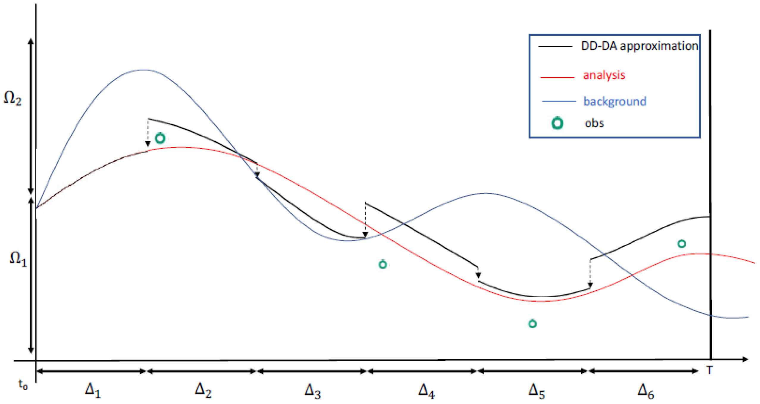
We introduce the 4D variational problem (see Figure 1).
Definition 2.
Let Ω R n and Δ R be the spatial domain and the time interval, respectively. The 4DVAR DA problem consists of computing the so-called analysis:
u D A = a r g m i n u R N p × N J ( u ) ,
in Ω × Δ with
J ( u ) = α u u M B 1 2 + G u y R 1 2 ,
where N p is the number of nodes in Ω R n ; n o b s , with n o b s < < N p , is the number of observations in Ω; N is the number of time instants in Δ; α is the regularization parameter; u 0 = { u 0 , j } j = 1 , , N p { u 0 ( x j ) } j = 1 , , N p R N p is the state at time t 0 ; the operator
M l 1 , l R N p × N p , l = 1 , , N ,
is the discretization of the linear approximation of M t l 1 , t l from t l 1 to t l ; the operator
M R N p × N p
is the discretization of the linear approximation of M , running from t 0 to t N ; the matrix
u M : = { u j , l M } j = 1 , , N p ; l = 1 , , N { u M ( x j , t l ) } j = 1 , , N p ; l = 0 , 1 , , N 1 R N p × N
is the solution of M, i.e., the background; y : = { y ( z j , t l ) } j = 1 , , n o b s ; l = 0 , 1 , , N 1 R n o b s × N : are the observations; H l R n o b s × N p , l = 0 , , N 1 : is the linear approximation of the observation mapping H ; G G N 1 R ( N × n o b s ) × N p is a block diagonal matrix G ( N × n o b s ) × ( N P × N ) such that
G = d i a g [ H 0 , H 1 M 0 , 1 , , H N 1 M N 2 , N 1 ] N > 1 ; H 0 N = 1 .
R = d i a g ( R 0 , R 1 , , R N 1 ) and B = V V T are the covariance matrices of the errors on observations and on the background, respectively.

The Space and Time DA—Driven Domain Decomposition Method

The strength of the DD-DA approach is the exploitation of the coupling between the DA functional and the underlying PDE model. The idea goes back to the work of Schwarz [17] on overlapping domains and to Parallel in Time (PinT) methods, introduced by Lions [18]. Briefly, in DD-DA, DA acts as a predictor for the PDE-based local model, providing the approximations needed to locally solve the initial value problems on each subdomain, concurrently. Leveraging Schwarz and PinT methods’ consistency constraints for PDEs-based models, the DD-DA framework iteratively adjusts local solutions by adding the contribution of adjacent subdomains to the local filter, along overlapping regions. As a consequence, this approach increases the accuracy of local solutions and it allows us to apply in parallel both the fine and coarse solvers.
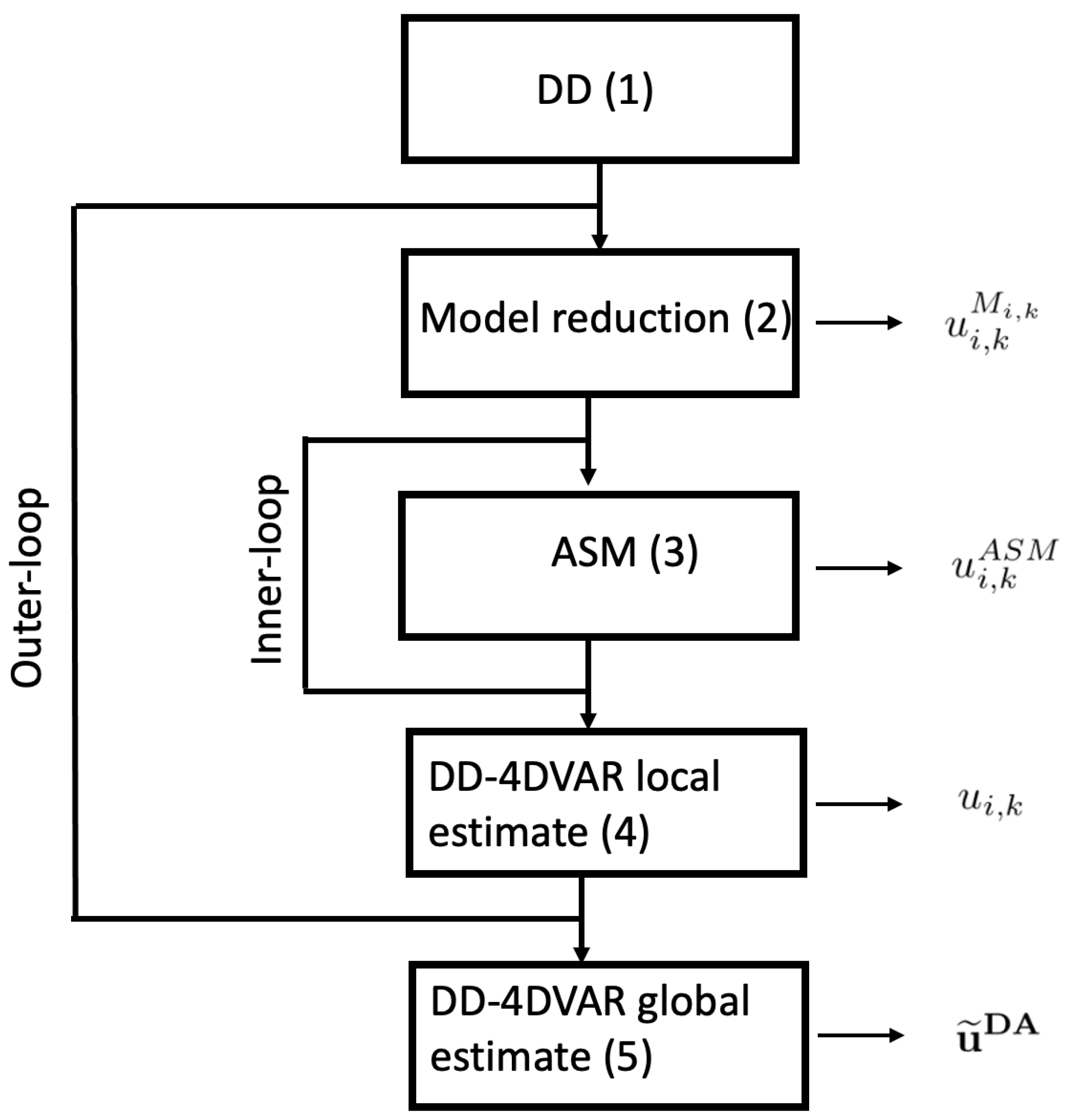
In the following, we briefly resume the method, according to its schematic description reported in Figure 2.
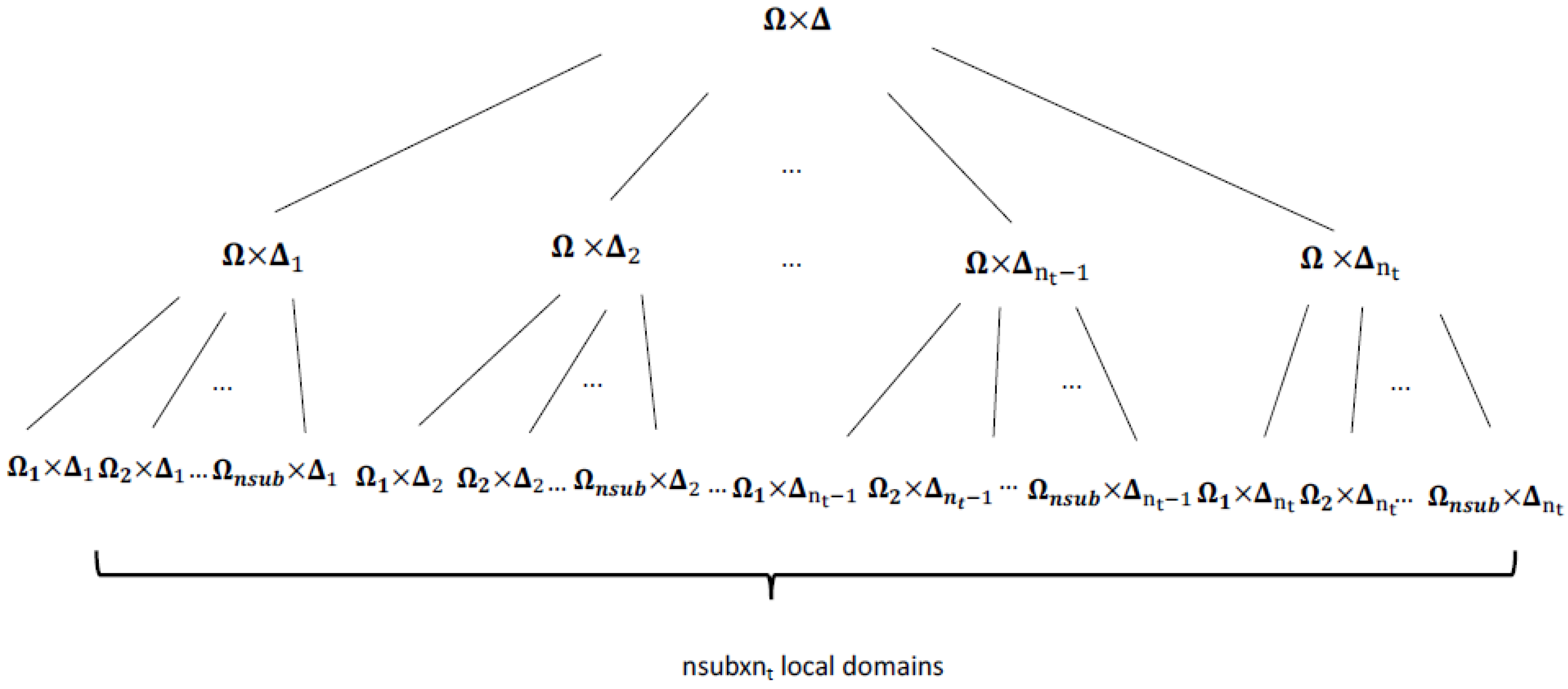
We describe the DD of Ω × Δ and of Ω I × Δ k . The DD of Ω × Δ consists in decomposing Ω R n into a set of subdomains Ω i such that:
Ω = i = 1 N s u b Ω i
and consequently we define the set J i , with cardinality a d i , made of indices of subdomains adjacent to Ω i ;
J i { 1 , , N s u b } and a d i = | J i | .
For i = 1 , , N s u b , we define the overlap regions Ω i j :
Ω i j : = Ω i Ω j j J i .
We define interfaces Γ i j , for i = 1 , , N s u b :
Γ i j : = Ω i Ω j j J i .
In the same way, time interval Δ R is decomposed into a sequence of intervals Δ k such that:
Δ = k = 1 N t Δ k .
Consequently, we define
{ Ω i × Δ k } i = 1 , , N s u b ; k = 1 , , N t
as local domains.
DD of Ω I × Δ K defined in (7): for i = 1 , , N s u b , the set
{ x i ˜ } i ˜ I i Ω i
is made of inner nodes of Ω i where I i is
I i : = ( i 1 ) N p N s u b + 1 , , i N p N s u b + δ 2
such that
I = i = 1 N s u b I i .
I is the set of indices of inner nodes in Ω defined in (5) and
δ : = | I i j |
where
I i j : = I i I j , j J i .
Selection of inner nodes belonging to the overlap regions { Ω i j } i = 1 , , N s u b , j J i proceeds in the same way. For i = 1 , , N s u b
Ω I i { x j ˜ } j ˜ I i j Ω i j , j J i
are the inner nodes of Ω i j . Consequently, for i = 1 , , N s u b , we define the cardinality of I i as the number of inner nodes of Ω i and we denote it as
N l o c : = | I i | = N p N s u b + δ 2 .
Finally, the selection of time values in { Δ k } k = 1 , , N t proceeds as follows. For k = 1 , , N t
Δ K k { t k ˜ } k ˜ K k Δ
are time values in Δ k where K k is defined as:
K k : = ( k 1 ) N N t , k N N t ,
where
K k K k + 1 = k N N t , k = 1 , , N t 1
and
N k : = | K k | = N N t
is the cardinality of K k , i.e., the number of time values belonging to K k , such that
K = k = 1 N t K k ,
where K is defined in (6).
Consistently with Definition 1, for i = 1 , , N s u b and k = 1 , , N t
Ω I i × Δ K k : = { ( x i ˜ , t k ˜ ) } i ˜ I i ; k ˜ K k Ω i × Δ k
is the local discrete domain/mesh.
For i = 1 , , N s u b and k = 1 , , N t , we pose
z i , k = { z ( i ˜ , k ˜ ) } i ˜ I i ; k ˜ K k R N l o c × N k
i.e., this is a vector defined on local domain Ω i × Δ k .
We define the restriction and extension operators underlying the DD method.
Definition 3 (Restriction Operator).
Given x R N p × N and z R N p × 1 , for i = 1 , , N s u b we define restriction of x to Ω i by
x / Ω i : = R i x = { x ( i ˜ , k ˜ ) } i ˜ I i , k ˜ K k R N l o c × 1
x / Ω i j : = R i j x = { x ( j ˜ , k ˜ ) } j ˜ I i j , k ˜ K k R δ × 1
and restriction of y to Ω i × Δ k by
z / ( Ω i × Δ k ) : = { z ( · , k ˜ ) } k ˜ K k / Ω i = R i { z ( · , k ˜ ) } k ˜ K k = { z ( i ˜ , k ˜ ) } i ˜ I i , k ˜ K k R N l o c × N k
z / ( Ω i j × Δ k ) : = { z ( · , k ˜ ) } k ˜ K k / Ω i j = R i j { z ( · , k ˜ ) } k ˜ K k = { z ( i ˜ , k ˜ ) } i ˜ I i j , k ˜ K k R N l o c × N k
where I i and I i j are, respectively, set of indices of inner nodes in Ω i and Ω i j , j J i .
Definition 4 (Extension operator).
If x R N l o c × N k , the Extension Operator (EO) is defined by
E O ( x ) : = R i T x = x ( i ˜ , k ˜ ) if ( i ˜ , k ˜ ) I i × K k 0 e l s e w h e r e
where R i T is the transpose of R i in (24) and E O ( x ) x E O .
For n = 0 , 1 , fixed, we now define the local model in each subdomain Ω i × Δ k , where i = 1 , , N s u b and k = 1 , , N t . If u i , k 0 : = { u M ( x i ˜ , t k ˜ ) } i ˜ I i j , k ˜ K k , is the background used as the initial value of the local model (see Figure 3), let u i , k M i , k , n + 1 be the solution of the problem ( P i , k M i , k , n ) i = 1 , N s u b , k = 1 , , N t where:
( P i , k M i , k , n ) i = 1 , N s u b , k = 1 , , N t : u i , k M i , k , n = M i , k u i , k 1 n + b i , k n , u i , k 1 n = u i , k 1 M i , k , n u i , k n / Γ i j = u j , k n / Γ i j , j J i
In (25) u i , k M and b i , k n are, respectively, the background in Ω i × Δ k and the vector accounting boundary conditions of Ω i and
M i , k : = M k / Ω i
is the restriction to Ω i of the matrix
M k M s ¯ k 1 , s ¯ k : = M s ¯ k 1 , s ¯ k 1 + 1 M s ¯ k 1 , s ¯ k .
where
s ¯ k : = j = 1 k 1 N j ( N 1 ) and s ¯ 0 : = 0
are the first index of Δ K K and Δ K 1 , respectively.
Let:
( P i , k n ) i = 1 , , N s u b , k = 1 , , N t : u i , k A S M , n = arg min u i , k n J i , k ( u i , k n )
be the local 4DVAR DA model with
J i , k ( u i , k n ) : = J ( u i , k n ) / ( Ω i × Δ k ) + 𝒪 i j .
We let
𝒪 i j : = j J i β j u i , k n / Ω i j u j , k n / Ω i j B i j 1 2
denote the overlapping operator in Γ i j , and
J i , k ( u i , k n ) / ( Ω i × Δ k ) : = α i , k u i , k n u i , k M i , k , n B i 1 + G i , k u i , k n y i , k R i 1 2
denote the restriction of J to Ω i × Δ k where G i , k is the restriction of G to Δ i × Ω k . Parameters α i , k and β j in (31) are the regularization parameters. For simplicity, we assume that α i , k = β j = 1 , for j J i .
The gradient of J i , k is [16]:
J i , k ( w i , k n ) = ( V i T ( G i , k ) T ( R i , k ) 1 G i , k V i + I i + a d i × B i j ) w i , k n c i + j J i B i j w j , k n ,
where
w i , k n = V i 1 ( u i , k n u i , k M i , k , n ) ,
d i = ( v i G i , k u i , k M i , k , n ) , c i = ( V i T ( G i , k ) T ( R i , k ) 1 d i )
where B i = V i V i T and I i is the identity matrix. The solution of ( P i , k n ) i = 1 , , N s u b , k = 1 , , N t is obtained by requiring that J i , k ( w i , k n ) = 0 . This requirement leads to the linear system:
A i , k w i , k n = c i j J i B i j w j , k n ,
where
A i , k = ( V i T ( G i , k ) T R i , k 1 G i , k V i + I i + a d i × B i j ) .
where a d i are the number of subdomains adjacent to Ω i .
For each n, the r.h.s. of (34) depends on unknown value w j , k n defined on those Ω i j , where j J i , which are adjacent to Ω i . According to the Additive Schwarz Method (ASM) [19] for r = 0 , 1 , , r ¯ we solve
A i , k w i , k r + 1 , n = c i j J i B i j w j , k r , n ,
by using Conjugate Gradient (CG) method where at step r + 1 , then Ω i receives w i , k r , n from Ω i j , where j J i , for computing the r.h.s. of (36) and finally it sends w i , k r + 1 , n to Ω i j , where j J i , for updating the r.h.s. of (36) is needed for the next iteration. At step 0, w i j , k 0 , n is an arbitrary initial value.
Finally, we pose
w i , k n w i , k r ¯ , n ,
and consequently we have that
u i , k A S M , n : = u i , k A S M , r ¯ .
The local solution update is performed by using (25) and (33):
u i , k n + 1 = u i , k M i , k , n + 1 + V i w i , k n = u i , k M i , k , n + 1 + [ u i , k A S M , n u i , k M i , k , n ] .
The global solution in Ω × Δ is
u ˜ DD DA , n : = i = 1 N s u b k = 1 N t ( u i , k n ) E O .
where ( u i , k n ) E O is the extension to Ω × Δ of local approximations computed in Ω i × Δ k . For simplicity, we let
u ˜ DD DA : = u ˜ DD DA , n ¯
be the solution in Ω × Δ .
Note that B i = R i B R i T and B i j : = B / Γ i j = R i B R i j T are the restrictions of the covariance matrix B , respectively, to subdomain Ω i and interface Γ i j defined in (17), while G i , k , and R i , k are the restriction of G k : = G s ¯ k and of R k : = d i a g ( R 0 , R 1 , , R s ¯ k ) to Ω i and, finally, u i , k M = R i u k M , u i , k n + 1 / Γ i j = R i j u i , k n + 1 , u j , k n / Γ i j = R i j u k n are the restriction of vectors u k b , u i , k n + 1 , u j , k n to Ω i and to Γ i j , for i = 1 , 2 , , N s u b and j J i .
In [11,12], the authors proved that the minimum of J can be obtained by patching together local solutions obtained as the minimum of local functions J i , k . In this way, the global minimum can be searched for among the global minima of the local functional.

3. Sensitivity Analysis

As already said, the core of the DD-DA approach is that the DA model acts as coarse/predictor operator to solve the local PDE model by providing the background values as initial conditions of the local PDE models. Then, we analyze the propagation of the errors with respect to the time direction. In the following, we use · = · 2 . We refer to z i , k 2 = { z i , k ( i ¯ , k ¯ ) } i ¯ I i , k ¯ K k 2 where z R N p × N and z i , k : = z / ( Ω i × Δ k ) and I i and K k are defined in (19) and (23), respectively.
Lemma 1.
[20] Let R > 0 and T 0 be two positive constant quantities. If we have a sequence E k which is such that for k = 1 , , N t :
| E k |   ( 1 + R ) | E k 1 | + T
then it holds:
| E k |   e N t R | E 1 | + e N t R 1 R T .
Definition 5.
Let u i , k n + 1 and u ˜ i , k n + 1 be, respectively, the numerical solution at step ( n + 1 ) in (38) and the corresponding floating point representation. Fixed n, for i = 1 , , N s u b , k = 1 , , N t let
R i , k n + 1 : = u i , k n + 1 u ˜ i , k n + 1
denote the round-off error in Ω i × Δ k .
From (25), the numerical solution at step ( n + 1 ) can be written as follows:
u i , k n + 1 = ( M i , k u k 1 n + 1 + b i , k n + 1 ) + [ u i , k A S M , n ( M i , k u i , k 1 n + b i , k n ) ] = M i , k u i , k 1 n + 1 + δ ( u i , k n )
consequently, the corresponding floating point representation is
u ˜ i , k n + 1 = M i , k u ˜ i , k 1 n + 1 + δ ( u ˜ i , k n ) + ρ k n + 1
where δ ( u i , k n ) : = ( u i , k A S M , n M i , k u i , k 1 n ) + ( b i , k n + 1 b i , k n ) and ρ k n + 1 is the local round-off error.
Fixed n + 1 , we have that
R i , k n + 1 = u i , k n + 1 u ˜ i , k n + 1 = M i , k u i , k 1 n + 1 + δ ( u i , k n ) M i , k u ˜ i , k 1 n + 1 δ ( u ˜ i , k n ) ρ k n + 1 M i , k u i , k 1 n + 1 M i , k u ˜ i , k 1 n + 1 + δ ( u i , k n ) δ ( u ˜ i , k n ) + | ρ k n + 1 | M i , k u k 1 n + 1 u ˜ k 1 n + 1 + u k A S M , n u ˜ k A S M , n + M i , k u i , k 1 n + b i , k n ( M i , k u ˜ i , k 1 n + b ˜ i , k n ) + b k n + 1 b ˜ i , k n + 1 + | ρ k n + 1 | ;
from (25) it is
b i , k n + 1 b ˜ i , k n + 1 = M i , k u i , k 1 n + 1 M i , k u ˜ i , k 1 n + 1
and according to [16] we let μ ( M i , k ) M i , k , where μ ( M i , k ) denotes the condition number of M i , k , then
R i , k n + 1 μ ( M i k ) u k 1 n + 1 u ˜ k 1 n + 1 + u k A S M , n u ˜ k A S M , n + u i , k M i , k , n u ˜ i , k M i , k , n + μ ( M i , k ) u k 1 n + 1 u ˜ k 1 n + 1 + μ ( M i , k ) u i , k 1 n u ˜ i , k 1 n + | ρ i k |
and in compact form
R k n + 1 2 μ ( M i , k ) R i , k 1 n + 1 + R i , k A S M , n + R i , k M , n + μ ( M i , k ) R i , k 1 n + | ρ i k |
where
R i , k A S M , n : = u i , k A S M , n u ˜ i , k A S M , n R i , k M i , k , n : = u i , k M i , k , n u ˜ i , k M i , k , n .
Using Lemma 1, with R = 2 μ ( M i , k ) 1 and H = R i , k A S M , n + R i , k M i , k , n + 1 + μ ( M i , k ) R i , k 1 n + ρ i k , it follows that:
R k n + 1   e N t R R i , 1 n + 1 + e N t R 1 R μ ( M i , k ) R i , k A S M , n + R i , k M i , k , n + μ ( M i , k ) R k 1 n + ρ i k .
then, it is
R k n + 1   e N t R R i , 1 n + 1 + e N t R 1 R R i , k A S M , n + R i , k M i , k , n + R i , k 1 n + e N t R 1 R ρ i k .
The upper bound in (43) is made of three terms: the first one represents the propagation of the error introduced on the first time interval, the second one represents the propagation of the error introduced at the previous step and the last term depends on the local round-off error. In particular, we note that, as expected, round-off error propagation grows with N t , i.e., the number of subdomains of Δ .

3.1. Convergence, Consistence and Stability of DD-DA Method

In [12], we proved the convergence of the outer loop, i.e.:
l i m n u ˜ DD DA , n + 1 u ˜ DD DA , n = 0
where u DA , n is defined in (39). The convergence of ASM is proved in [19].

3.1.1. Consistence

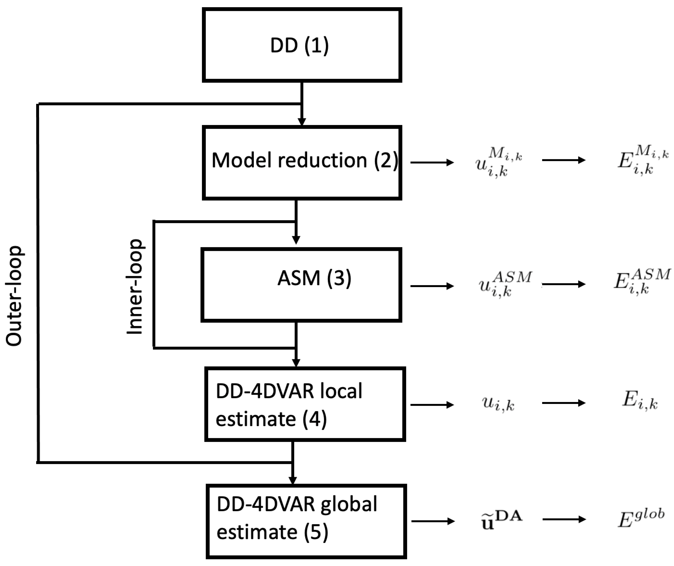
We analyze the consistence in terms of the local truncation errors E i , k M i , k , E i , k A S M , E i , k and E g , which are reported in Figure 4.
Similar to [21], local truncation errors E i , k M i , k , E i , k A S M , E i , k in Ω i × Δ k and E g l o b in Ω × Δ are defined as the remainder after the solutions u M of the model (1) and the solution u DA of the 4D-DA problem (8) are substituted into the discrete models. To this aim, we give the following definitions.
Definition 6.
We define
u M M : = M · { u M ( x i , t k ) } i ˜ I ; k ˜ K
as the approximation in Ω × Δ of u M , defined in (1), obtained by replacing u M evaluated in Ω I × Δ K and defined in (1), into M, which is defined in (11).
Definition 7 (Local truncation errors in Ω i × Δ k ).
i = 1 , , N s u b and k = 1 , , N t , at iteration n ¯ , we define
E i , k M i , k , n ¯ : = u M M / ( Ω i × Δ k ) u i , k M i , k , n ¯
as the local truncation error of M i , k restricted to Ω i × Δ k ;
E i , k A S M , n ¯ : = u DA / ( Ω i × Δ k ) u i , k A S M , n ¯
as the local truncation error of ASM restricted to Ω i × Δ k ;
E i , k n ¯ : = u DA / ( Ω i × Δ k ) u i , k n ¯
as the local truncation error of DD-DA restricted to Ω i × Δ k ;
E g l o b : = u DA u ˜ DD DA
as the local truncation error of DD-DA in Ω × Δ .
The DD-4DVAR method needs few iterations of the outer loop over n to update the approximation in (38). Consequently, in the following analysis, we neglect the dependency on n ¯ of u i , k M i , k , n ¯ , u i , k A S M , n ¯ and u i , k n , defined, respectively, in (25), (29) and (38) and E i , k M i , k , n ¯ , E i , k A S M , n ¯ and E i , k n ¯ in Ω i × Δ k , defined, respectively, in (46), (47) and (48).
For i = 1 , , N s u b and k = 1 , , N t , we pose
u ˜ i , k : = u i , k n ¯ .
From (50), the approximation in Ω × Δ defined in (40) becomes
u ˜ DD DA = i = 1 N s u b k = 1 N t u ˜ i , k E O .
For i = 1 , , N s u b and k = 1 , , N t , we pose
u i , k A S M = u i , k A S M , n ¯ ; u i , k M i , k = u i , k M i , k , n ¯ ; u i , k = u i , k n ¯ .
Consequently, from (52) we pose
E i , k M i , k = E i , k M i , k , n ¯ ,
as the local model truncation error in Ω i × Δ k ;
E i , k A S M = E i , k A S M , n ¯ ,
as the local ASM truncation error in Ω i × Δ k in (47);
E i , k = E i , k n ¯ .
as the local truncation error Ω i × Δ k in (48).
We introduce the definition of consistency of the DD-DA method. We pose · = · 2 . (We refer to z i , k 2 = { z i , k ( i ¯ , k ¯ ) } i ¯ I i , k ¯ K k 2 where z R N p × N and z i , k : = z / ( Ω i × Δ k ) and I i and K k are defined in (19) and (23), respectively).
Definition 8 (Consistency of DD-DA method).
The DD-DA method is said to be consistent if
lim Δ x , Δ t 0 E g = 0
where
Δ x : = m a x i = 1 , , N s u b ( Δ x ) i
and { ( Δ x ) i } i = 1 , , N s u b are spatial-step sizes of M i , k ;
Δ t : = m a x k = 1 , , N t ( Δ t ) k
and { ( Δ t ) k } k = 1 , , N t are time-step sizes of M i , k .
In order to prove the consistency, we perform the analysis of local truncation errors E i , k M i , k , E i , k A S M , E i , k and E g l o b , defined, respectively, in (53), (54), (55) and (49).
Assumption 1.
(Local truncation error of Model in Ω i × Δ k ) Let
E i , k M i , k = 𝒪 ( ( Δ x ) i p + ( Δ t ) k q ) , ( i , k ) { 1 , , N s u b } × { 1 , , N t }
be the local truncation error defined in (53) where ( Δ x ) i and ( Δ t ) k are spatial and temporal step sizes of M i , k , defined in (26), and p and q are the order of convergence in space and in time. In the experimental results (see Section 4), in order to discretize the Shallow Water Equations (SWEs) model, we consider Lax–Wendroff scheme [22]. Hence, in that case, p = q = 2 .
Lemma 2 (Local truncation error of ASM in Ω i × Δ k ).
Let us consider the following quantities: σ 0 2 , observational error variance; B i = V i V i T , restriction to Ω i of covariance matrices of the error on background; G i , k , restriction to Ω i × Δ k of matrix G defined in (13); a d i , number of subdomains adjacent to Ω i , defined in (15); B i j = V i j V i j T , restriction to Ω i j of the covariance matrix of the error on the background; μ ( V i ) , μ ( G i , k ) , μ ( M i , k ) and μ ( V i j ) , condition number of V i , G i , k , M i , k and V i j , respectively. Then, i = 1 , , N s u b and k = 1 , , N t , it holds that:
E i , k A S M μ i , k D D D A × E i , 1 A S M
where
μ i , k D D D A : = 1 + 1 σ 0 2 μ 2 ( V i ) μ 2 ( G i , k ) + a d i × μ 2 ( V i j ) μ ( M i , k ) .
Proof. 
As in [16], it is
u D A / ( Ω i × Δ k ) u i , k A S M   μ ( J i , k ) μ ( M i , k ) × u DA / ( Ω i × Δ 1 ) u i , 1 A S M
where u DA / ( Ω i × Δ 1 ) u i , 1 A S M is the error in Ω i × Δ 1 . As proved in [16], it is
μ ( J i , k ) = μ ( A i , k )
where J i , k and A i , k are, respectively, defined in (30) and (35), and by using triangle inequality, it is
μ ( A i , k ) 1 + 1 σ 0 2 μ 2 ( V i ) μ 2 ( G i , k ) + a d i × μ ( B i j )
                1 + 1 σ 0 2 μ 2 ( V i ) μ 2 ( G i , k ) + a d i × μ 2 ( V i j ) ,
From (59) and (61), the (57) follows. □
Theorem 1.
(Local truncation error in Ω i × Δ k ) i = 1 , , N s u b ; k = 1 , , N t , it holds that:
E i , k μ i , k D D D A × E i , 1 A S M + 2 × E i , k M i , k
where μ i , k D D D A is defined in (58).
Proof. 
From (52) and (38), E i , k defined in (55) can be rewritten as follows:
E i , k : = u DA / ( Ω i × Δ k ) u i , k = u DA / ( Ω i × Δ k ) u i , k M i , k , n ¯ ( u i , k A S M , n ¯ 1 u i , k M i , k , n ¯ 1 ) ;
by using the triangle inequality, it is
E i , k   u DA / ( Ω i × Δ k ) u i , k A S M , n ¯ + u i , k M i , k , n ¯ 1 u i , k M i , k , n ¯ ;
as consequence of Lemma 2 and (54), we have that
E i , k μ i , k D D D A × E i , 1 A S M + u i , k M i , k , n ¯ 1 u i , k M i , k , n ¯
where E i , 1 A S M is defined in (54) and μ i , k D D D A is defined in (58). In particular, by adding and subtracting u M M / ( Ω i × Δ k ) in u i , k M i , k , n ¯ 1 u i , k M i , k , n ¯ , we obtain:
u i , k M i , k , n ¯ 1 u i , k M i , k , n ¯ = ( u i , k M i , k , n ¯ 1 u M M / ( Ω i × Δ k ) ) + ( u M M / ( Ω i × Δ k ) u i , k M i , k , n ¯ )
and by using the triangle inequality
u i , k M i , k , n ¯ 1 u i , k M i , k , n ¯ u i , k M i , k , n ¯ 1 u M M / ( Ω i × Δ k ) + u M M / ( Ω i × Δ k ) u i , k M i , k , n ¯ = E i , k M i , k , n ¯ + E i , k M i , k , n ¯ 1 .
{ u ˜ DD DA , n } n N is a convergent sequence, then it is a Cauchy sequence. From (39), we find that { u i , k M i , k , n } n N is also a Cauchy sequence, i.e.,
ϵ > 0 N > 0 : u i , k M i , k , n u i , k M i , k , m   ϵ n , m > N .
In particular, the equation (67) is true for n = n ¯ and m = n ¯ 1 , assuming that n ¯ is large enough. Consequently, we can neglect the dependency on the outer loop in E i , k M i , k , n ¯ and E i , k M i , k , n ¯ 1 in (66), i.e.,
u i , k M i , k , n ¯ 1 u i , k M i , k , n ¯   2 E i , k M i , k
where E i , k M i , k is defined in (53). From (65), (66) and (68), we obtain the thesis in (63). □
Lemma 3.
If e 0 , the error on initial condition of M in (11) is equal to zero, i.e.,
e 0 = 0
then
E i , k c ( ( Δ x ) i p + ( Δ t ) k q )
where E i , k is the local truncation error defined in (55) and c is positive constant independent on DD.
Proof. 
By applying Theorem 1 to E i , 1 A S M on Ω i × Δ 1 , we obtain
E i , 1 A S M F i , 1 e 0 / Ω i .
where F i , 1 is defined in (58) and e 0 / Ω i is the restriction of e 0 to Ω i . As it is e 0 / Ω i = 0 , then by replacing e 0 / Ω i = 0 in (71), it results that
E i , 1 A S M = 0
consequently, we have that
E i , k A S M = 0 .
From (73), (56) and (63), we obtain the thesis in (70). □
Theorem 2.
(Truncation error in Ω × Δ ) Under the assumption of Lemma 3 in (69), the truncation error in Ω × Δ is such that
E g l o b c ( N s u b N t ) [ ( Δ x ) p + ( Δ t ) q ] ,
where c > 0 is a positive constant independent on DD.
Proof. 
From (51), it results that E g l o b , which is defined in (49), can be rewritten as follows:
E g l o b : = u DA u ˜ DD DA = u DA i = 1 N s u b k = 1 N t u ˜ i , k
by applying the restriction and extension operator (Definitions 3 and 4) to u DA , we obtain
E g l o b = i = 1 N s u b k = 1 N t ( u DA / ( Ω i × Δ k ) ) E O u ˜ i , k
by using the triangle inequality, it is
E g = i = 1 N s u b k = 1 N t ( u DA / ( Ω i × Δ k ) ) E O u ˜ i , k i = 1 N s u b k = 1 N t ( u i , k DA ) E O u ˜ i , k = i = 1 N s u b k = 1 N t E i , k
where E i , k is defined in (55). From Lemma 3, we have
i = 1 N s u b k = 1 N t E i , k c i = 1 N s u b k = 1 N t ( ( Δ x ) i p + ( Δ t ) k q ) = c N t i = 1 N s u b ( Δ x ) i p + N s u b k = 1 N t ( Δ t ) k q ,
and consequently
E g l o b c N t i = 1 N s u b ( Δ x ) i p + N s u b k = 1 N t ( Δ t ) k q .
By defining
Δ x : =   m a x i = 1 , , N s u b ( Δ x ) i Δ t : =   m a x k = 1 , , N t ( Δ t ) k
we obtain
E g l o b c N t i = 1 N s u b ( Δ x ) i p + N s u b k = 1 N t ( Δ t ) k q c N t i = 1 N s u b ( Δ x ) p + N s u b k = 1 N t ( Δ t ) q c ( N s u b N t ) [ ( Δ x ) p + ( Δ t ) q ] .
Hence, the (74) is proved. □

3.1.2. Stability

Now, we prove the stability of the method with respect to the time direction, and assuming that the predictive model is stable. We will perform SA by obtaining worst-case error bounds with the aid of the condition number.
We assume that the discrete scheme applied to the model M in (1) is stable, i.e., D > 0 such that
u M v M   D e 0 ,
where u M is the computed solution of M in (11) and v M is the solution of M ¯ , where M ¯ is obtained by adding error e 0 to initial condition of M. For simplicity of notations in the sequel, we omit any subscripts of M .
Definition 9 (Propagation error from Δ k 1 to Δ k ).
Let v ˜ DD DA be the solution in Ω × Δ computed by adding the perturbation e k to the initial condition of P i , k M i , k , n , defined in (25). We define
E ¯ k : = u ˜ DD DA / Δ k v ˜ DD DA / Δ k
as the propagation error from Δ k 1 to Δ k .
Theorem 3 (Stability).
If the error on initial condition of M in (11), is equal to zero, i.e.,
e 0 = 0
then, k = 1 , , N t C k > 0 such that
E ¯ k C k e ¯ k
where C k is a constant depending on the model and on the ASM; e ¯ k is the perturbation on the initial condition of P i , k M i , k , defined in (25).
Proof. 
To simplify the notations in the proof, we consider e ¯ k = e ¯ , k = 1 , , N t . From (38), (52) and using the triangle inequality, we obtain
E ¯ k : = u ˜ DD DA / Δ k v ˜ DD DA / Δ k   ( u i , k M i , k , n ¯ ) E O / Δ k ( v i , k M i , k , n ¯ ) E O / Δ k +   ( u i , k M i , k , n ¯ 1 ) E O / Δ k ( v i , k M i , k , n ¯ 1 ) E O / Δ k +   ( u i , k A S M , n ¯ ) E O / Δ k ( v i , k A S M , n ¯ ) E O / Δ k .
From (67) and (54), we can neglect the dependency on n ¯ , i.e.,
E ¯ k 2 ( u i , k M i , k ) E O / Δ k ( v i , k M i , k ) E O / Δ k   +   ( u i , k A S M ) E O / Δ k ( v i , k A S M ) E O / Δ k .
From the assumption on the model, we may say that D ¯ > 0 such that
( u i , k M i , k ) E O / Δ k ( v i , k M i , k ) E O / Δ k   D ¯ e 0 .
where e 0 is the error on the initial condition of M in (11). By adding and subtracting u DA / Δ k to ( u i , k A S M ) E O / Δ k ( v i , k A S M ) E O / Δ k and using the triangle inequality, it is
( u i , k A S M ) E O / Δ k ( v i , k A S M ) E O / Δ k     u DA / Δ k ( u i , k A S M ) E O / Δ k +   u DA / Δ k ( v i , k A S M ) E O / Δ k .
From (83) and (57), we obtain
( u i , k A S M ) E O / Δ k ( v i , k A S M ) E O / Δ k   μ k D D D A E 1 A S M + μ ¯ k D D D A E ¯ 1 A S M
where
E 1 A S M =   u DA / Δ 1 ( u i , 1 A S M ) E O / Δ 1 E ¯ 1 A S M =   u DA / Δ 1 ( v i , 1 A S M ) E O / Δ 1 .
and
μ k D D D A : = 1 + 1 σ 0 2 μ 2 ( V ) μ 2 ( G / Δ k ) μ ( M / Δ k ) μ ¯ k D D D A : = 1 + 1 σ 0 2 μ 2 ( V ) μ 2 ( G / Δ k ) μ ( M ¯ / Δ k )
with σ 0 denoting the observational error variance, B = V V T the covariance matrix of the error on the background to Ω , G the matrix defined in (13), M defined in (11) and M ¯ the discrete model obtained by considering initial error e 0 on the initial condition of M. By applying (57) to E 1 A S M and E ¯ 1 A S M in (85), we obtain
( u i , k A S M ) E O / Δ k ( v i , k A S M ) E O / Δ k   μ k D D D A μ 1 D D D A e 0 + μ ¯ k D D D A μ ¯ k D D D A e ¯ .
From (81), (82) and (84), it is
E ¯ k 2 D ¯ × e 0 + μ k D D D A μ 1 D D D A e 0 + μ ¯ k D D D A μ ¯ 1 D D D A e ¯
and from the hypothesis in (79), we obtain
E ¯ k μ ¯ k D D D A μ ¯ 1 D D D A e ¯
Consequently, for k = 1 , , N t , we find that C k > 0 such that
E ¯ k C k e ¯
where
C k : = μ ¯ k D D D A μ ¯ 1 D D D A .
The thesis is proved. □
From Theorem 3, we obtain the stability of DD-DA.
Remarkfrom Lemma 2 it follows that the quantity μ i , k D D D A can be regarded as the condition number of local problems restricted to the space-time directions. Further, in Theorem 3, we study the propagation error along the time direction according to the forward error analysis. As a consequence, we may say that μ k D D D A can be regarded as the condition number of local problems restricted to the time direction. In [16], the authors apply the SA to the reduced DA functional obtained by applying domain decomposition across space. The results in [16] proved that Tikhonov regularization revealed to be more appropriate than truncation of EOFs to improve the conditioning of the covariance matrix. The results obtained in the present study complement the study in [16].

4. Validation Analysis

The validation is performed mapping the space-time domain (Figure 5) on the high performance hybrid computing architecture of the SCoPE (Sistema Cooperativo Per Elaborazioni scientifiche multidiscipliari) data center, which is located in the University of Naples Federico II. Specifically, the architecture is composed of eight nodes that consist of distributed memory DELL M600 blades. The blades are connected by a 10 Gigabit Ethernet technology and each of them is composed of 2 Intel [email protected] GHz quadcore processors sharing the same local 16 GB RAM memory for a number of 8 cores per blade and of 64 total cores. Experimental results allow us to verify that the experimental order of consistency corresponds to the theoretical one obtained in Theorem 2 and that the local problems are well-conditioned. We consider the following experimental setup.
4DVAR DA setup.
  • Ω = ( 0 ,   1 ) R : spatial domain;
  • Δ = [ 0 ,   1.5 ] R : time interval;
  • N p = 640 : numbers of inner nodes of Ω defined in (5);
  • N = 9 ,   20 : numbers of occurrences of time in Δ ;
  • n o b s = 64 : number of observations considered at each step l = 0 , 1 , , N ;
  • y R N × n o b s : observations vector at each step l = 0 , 1 , , N . Observations are obtained choosing (randomly) these values among the values of the state function (the so called background) and perturbing (randomly) them. (We choice the observation in this way because the experimental set up is aimed to validate the sensitivity analysis of DD-DA instead of the reliability of DD-DA method);
  • H l R n o b s × N p : piecewise linear interpolation operator whose coefficients are computed using the nodes of Ω nearest to the observation values;
  • G R N × n o b s × N p : obtained as in (13) from the matrix H l , l = 0 , 1 , , N ;
  • σ m 2 = 0.5 , σ 0 2 = 0.5 : model and observational error variances;
  • B B l = σ m 2 C : covariance matrix of the error of the model at each step l = 0 , 1 , , N , where C R N p × N p denotes the Gaussian correlation structure of the model errors in (91);
  • R l = σ 0 2 I n o b s , n o b s R n o b s × n o b s : covariance matrix of the errors of the observations at each step l = 0 , 1 , , N 1 .
  • R R N × n o b s × N × n o b s : a diagonal matrix obtained from the matrices R l , l = 0 , 1 , , N 1 .
DD-DA setup: we consider the following setup:
  • p = N s u b × N t : number of cores;
  • N s u b : number of spatial subdomains;
  • N t = 4 : number of time intervals;
  • δ : number of inner nodes of overlap regions defined in (20);
  • N l o c : inner nodes of subdomains defined in (22);
  • Δ x and Δ t : spatial and temporal step sizes of M i , k defined in (26);
  • C : = { c i , j } i , j = 1 , , N p R N p × N p : the Gaussian correlation structure of the model error where
    c i , j = ρ | i j | 2 , ρ = e x p Δ x 2 2 , | i j | < N p / 2 for i , j = 1 , , N p .
Given δ , N s u b , N t , we introduce
e Δ x , Δ t p : = u DA u ˜ DD DA 2 ,
where u DA denotes the minimum of the 4DVAR (global) functional J in (9) while u ˜ DD DA is obtained by gathering all minima of the local 4DVar functionals J i , k , in (30), by considering different values of δ defined in (20). u DA R N p × N is computed by running the DD-DA algorithm for N s u b = 1 , while u ˜ DD DA R N p × N is computed by gathering local solutions obtained by running the DD-DA algorithm for different values of N s u b > 1 and with δ 0 , as shown in Figure 6.
In the following, we present the experimental results of the consistency and the stability analysis by considering the initial boundary problem of the Shallow Water Equations (SWEs) in 1D. The discrete model is obtained using the Lax–Wendroff scheme [22] on Ω × Δ where the orders of convergence in space and time are equal to 2.
  • Consistency. From Table 1, we obtain
    e Δ x d , Δ t d p e Δ x , Δ t p d 2 d = 1 , 2 , 4 , 6 , 8 , 10 .
    As shown in Table 1 and Figure 7, the experimental order of consistency corresponds to the theoretical one obtained in Theorem 2.
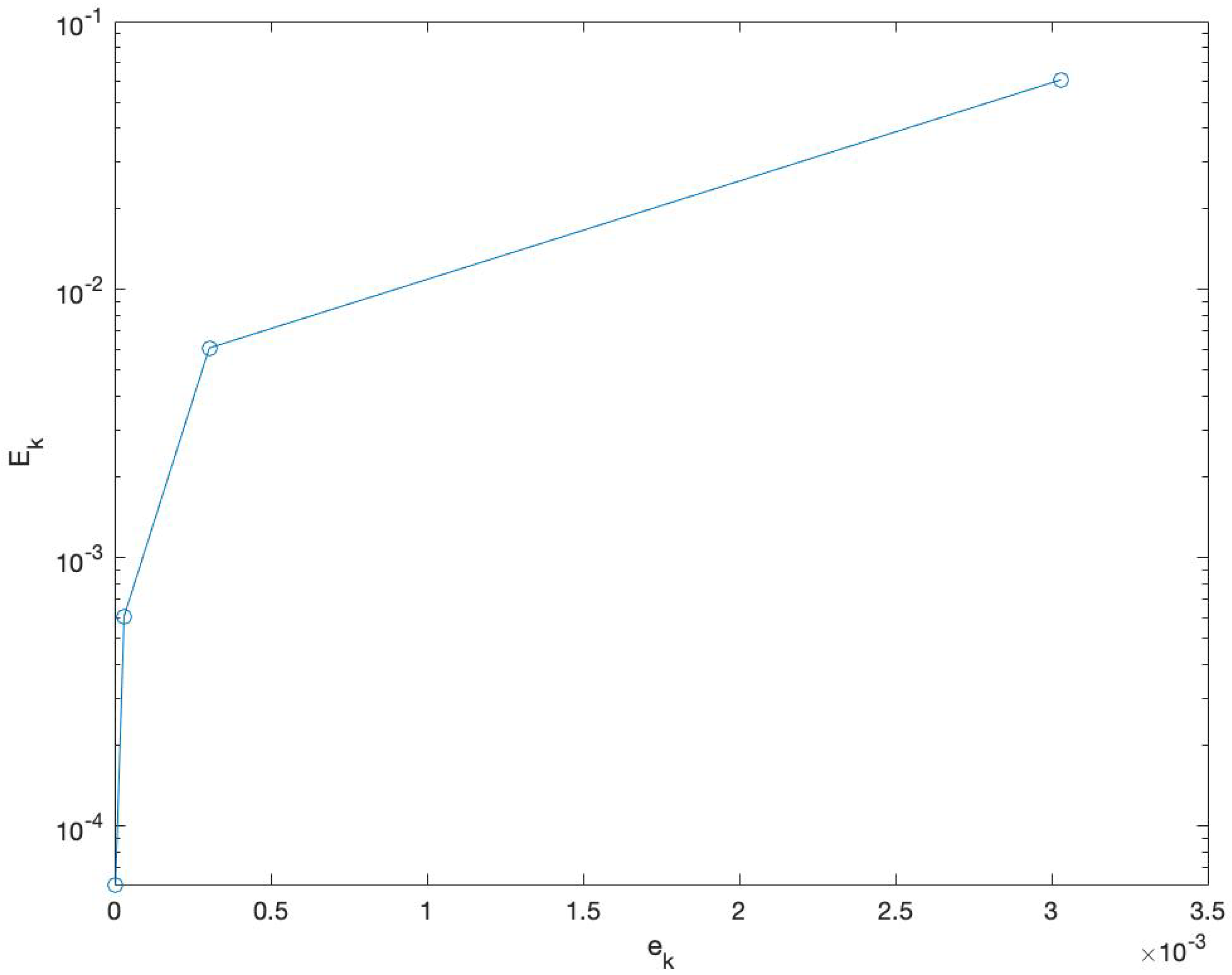
  • Stability. In Table 2 and Figure 8, we report values of E ¯ k for different values of the perturbation e ¯ k on the initial condition of P i , k M i , k defined in (25). Then, we may estimate C k in (90). In particular, we found that
    C k 2.00 × 10 1 k = 1 , , N t .
    Consequently, the local problems with initial boundary problem of SWEs 1D, are well-conditioned with respect to the time direction.

5. Conclusions

This work concerns the sensitivity analysis for large scale DA problems that need parallel solutions. We feel that the whole analysis of uncertainties becomes crucial for the emerging approaches integrating DA with deep learning approaches. We derived and discussed the main sources of errors of the parallel DD-DA framework. We prove that the order of consistence depends on the order of local models and introduce the condition number of local problems. As the core of such a parallel approach is that the DA model acts as coarse/predictor operator solving the local PDE model, we analyze error propagation with respect to time direction. Validation analysis confirms that the experimental order of consistency corresponds to the theoretical one. Finally, we note that the SA results in [16] proved that Tikhonov regularization revealed to be more appropriate than truncation of EOFs to improve the conditioning of the covariance matrix. Our results here complement the study in [16] and we may conclude that the same findings hold true for DD-DA, too.

Author Contributions

L.D.: supervision; methodology; formal analysis;conceptualization; writing, review and editing; R.C.: Data curation; Formal analysis; Methodology; Software; visualization; investigation; writing—original draft. All authors have read and agreed to the published version of the manuscript.

Funding

This research received no external funding.

Data Availability Statement

The data presented in this study are available on request from the corresponding author.

Conflicts of Interest

The author declares no conflict of interest.

References

  1. Ghil, M.; Malanotte-Rizzoli, P. Data assimilation in meteorology and oceanography. Adv. Geophys. 1991, 33, 141–266. [Google Scholar]
  2. Navon, I.M. Data Assimilation for Numerical Weather Prediction: A Review. In Data Assimilation for Atmospheric, Oceanic and Hydrologic Applications; Park, S.K., Xu, L., Eds.; Springer: Berlin/Heidelberg, Germany, 2009. [Google Scholar]
  3. Blum, J.; Le Dimet, F.; Navon, I. Data Assimilation for Geophysical Fluids. In Handbook of Numerical Analysis; Elsevier Inc. (Branch Office): San Diego, CA, USA, 2005; Volume XIV, Chapter 9. [Google Scholar]
  4. D’Elia, M.; Perego, M.; Veneziani, A. A variational data assimilation procedure for the incompressible Navier-Stokes equations in hemodynamics. J. Sci. Comput. 2012, 52, 340–359. [Google Scholar] [CrossRef]
  5. D’Amore, L.; Murli, A. Regularization of a Fourier series method for the Laplace transform inversion with real data. Inverse Probl. 2012, 18, 1185–1205. [Google Scholar]
  6. Cohn, S.E. An introduction to estimation theory (data assimilation in meteology and oceanography: Theory and practice). J. Meteorol. Soc. Jpn. Ser. II 1997, 75, 257–288. [Google Scholar] [CrossRef] [Green Version]
  7. Nichols, N.K. Mathematical concepts of data assimilation. In Data Assimilation; Springer: Berlin/Heidelberg, Germany, 2010; pp. 13–39. [Google Scholar]
  8. Zhang, Z.; Moore, J.C. Mathematical and Physical Fundamentals of Climate Change; Elsevier: Amsterdam, The Netherlands, 2014. [Google Scholar]
  9. D’Amore, L.; Marcellino, L.; Mele, V.; Romano, D. Deconvolution of 3D fluorescence microscopy images using graphics processing units, Lecture Notes in Computer Science. In Proceedings of the 2012 9th International Conference on Parallel Processing and Applied Mathematics, PPAM 2011, Torun, Poland, 11–14 September 2011; Springer: Berlin/Heidelberg, Germany, 2011; Volume 7203, pp. 690–699. [Google Scholar]
  10. Antonelli, L.; Carracciuolo, L.; Ceccarelli, M.; D’Amore, L.; Murli, A. Total variation regularization for edge preserving 3D SPECT imaging in high performance computing environments, Lecture Notes in Computer Science. In Proceedings of the 2002 International Conference on Computational Science, ICCS 2002, Amsterdam, The Netherlands, 21–24 April 2002; Springer: Berlin/Heidelberg, Germany, 2002; Volume 2330, pp. 171–180. [Google Scholar]
  11. D’Amore, L.; Cacciapuoti, R. Model reduction in space and time for ab initio decomposition of 4D variational data assimilation problems. Appl. Numer. Math. 2021, 160, 242–264. [Google Scholar] [CrossRef]
  12. D’Amore, L.; Costantinescu, E.; Carracciuolo, L. A scalable space-and-time domain decomposition approach for solving large scale non linear regularized inverse ill posed problems in 4D Variational Data Assimilation. J. Sci. Comput. 2022, 91, 59. [Google Scholar] [CrossRef]
  13. D’Amore, L.; Arcucci, L.; Carracciuolo, L.; Murli, A. DD-ocean var: A domain decomposition fully parallel data assimilation software for the mediterranean forecasting system. In Proceedings of the 2013 13th Annual International Conference on Computational Science, ICCS 2013, Barcelona, Spain, 7–13 June 2013; Elsevier: Amsterdam, The Netherlands, 2013; Volume 18, pp. 1235–1244. [Google Scholar]
  14. Arcucci, R.; D’Amore, L.; Carracciuolo, L. On the problem-decomposition of scalable 4D-Var Data Assimilation models. In Proceedings of the 2015 International Conference on High Performance Computing and Simulation, HPCS 2015, Amsterdam, The Netherlands, 20–24 July 2015; pp. 589–594. [Google Scholar]
  15. Cacuci, D. Sensitivity and Uncertainty Analysis; Chapman & Hall/CRC: New York, NY, USA, 2003. [Google Scholar]
  16. Arcucci, R.; D’Amore, L.; Pistoia, J.; Toumi, R.; Murli, A. On the variational data assimilation problem solving and sensitivity analysis. J. Comput. Phys. 2017, 335, 311–326. [Google Scholar] [CrossRef] [Green Version]
  17. Schwarz, H.A. Ueber einige Abbildungsaufgaben. De Gruyter 2009, 1869, 105–120. [Google Scholar] [CrossRef]
  18. Lions, P.L. On the Schwarz alternating method. III: A variant for nonoverlapping subdomains. In Proceedings of the Third International Conference on Domain Decomposition Methods, Houston, TX, USA, 20–22 March 1989; SIAM: Philadelphia, PA, USA, 1990; Volume 6, pp. 202–223. [Google Scholar]
  19. Dryja, M.; Widlund, O.B. Some domain decomposition algorithms for elliptic problems. In Iterative Methods for Large Linear Systems (Austin, TX, 1988); Academic Press: Boston, MA, USA, 1990; pp. 273–291. [Google Scholar]
  20. Dalquist, G.; Bjiork, A. Numerical Methods; Dover Publication: Mineola, NY, USA, 1974. [Google Scholar]
  21. Dahlquist, G. Convergence and stability in the numerical integration of ordinary differential equations. Math. Scand. 1956, 4, 33–53. [Google Scholar] [CrossRef] [Green Version]
  22. LeVeque, R.J.; Leveque, R.J. Numerical Methods for Conservation Laws; Springer: Berlin/Heidelberg, Germany, 1992; Volume 132. [Google Scholar]
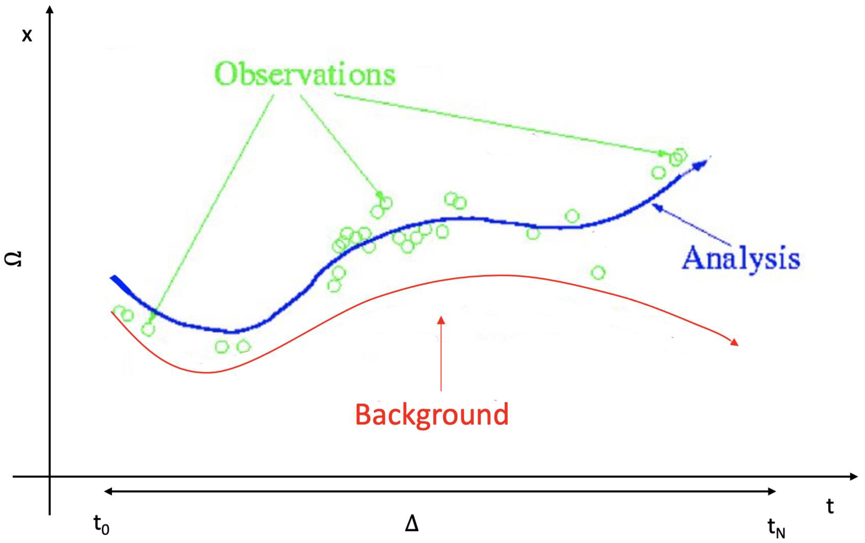
Figure 1. The 4D variational problem.
Axioms 12 00541 g001
Figure 2. Schematic description of DD-DA algorithm. DD, local model, ASM (Additive Schwarz Method), DD-DA local solutions and global solution are identified. The Arabic numbers in parentheses refer to the corresponding module described in Section 2. For each module, we report its solution.
Axioms 12 00541 g002
Figure 3. Initial conditions of local models in Ω i × Δ k .
Axioms 12 00541 g003
Figure 4. Local truncation errors related to each module of DD-DA.
Axioms 12 00541 g004
Figure 5. Space-time domain decomposition.
Axioms 12 00541 g005
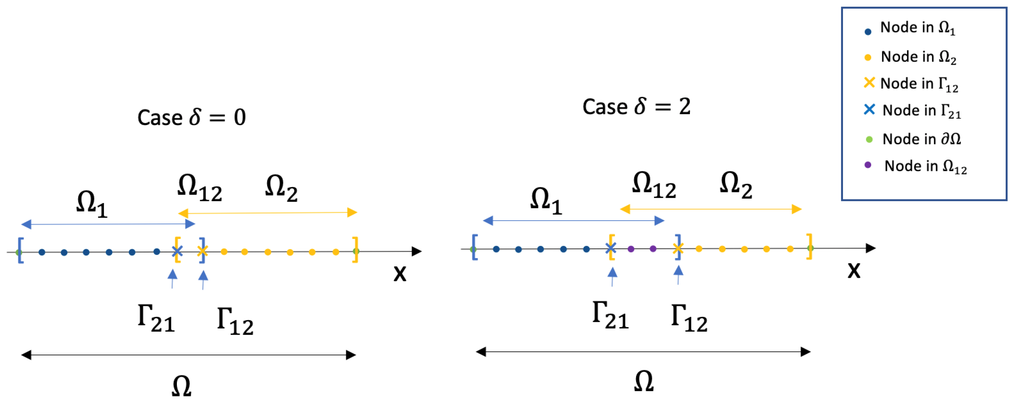
Figure 6. Decomposition of the spatial domain Ω R in two subdomains { Ω i } i = 1 , 2 by identifying overlap region Ω 12 defined in (16) and interfaces Γ 12 and Γ 21 defined in (17). On the left case δ = 0 , i.e., no inner nodes in Ω 12 , on the right case δ = 2 , i.e., two inner nodes in overlap region Ω 12 .
Axioms 12 00541 g006
Figure 7. Values of e Δ x d , Δ t d p (orange dashed line) and e Δ x , Δ t p d 2 (blue full line) for d = 1 , 2 , 4 , 6 , 8 , 10 reported in Table 1.
Axioms 12 00541 g007
Figure 8. Values ( e ¯ k , E ¯ k ) as reported in Table 2.
Axioms 12 00541 g008
Table 1. We fix N p = 640 , the number of inner nodes in Ω , N = 9 the number of time values in Δ , N s u b = 4 the number of spatial subdomain and N t = 4 time intervals. We report the values of e p , which is defined in (92), for different values of Δ x and Δ t , the spatial and temporal step sizes of M i , k defined in (26).
d Δ x d Δ t d e Δ x d , Δ t d p e Δ x , Δ t p d 2
1 7.87 × 10 3 1.09 × 10 1 1.53 × 10 2 1.53 × 10 2
2 3.92 × 10 3 5.47 × 10 2 9.01 × 10 4 3.83 × 10 3
4 1.96 × 10 3 2.74 × 10 2 6.45 × 10 4 9.56 × 10 4
6 1.30 × 10 3 1.83 × 10 2 3.65 × 10 4 2.39 × 10 4
8 9.78 × 10 4 1.37 × 10 2 3.99 × 10 4 4.25 × 10 4
10 7.81 × 10 4 1.10 × 10 2 3.77 × 10 4 1.53 × 10 4
Table 2. We fix N p = 640 , the number of inner nodes in Ω , N = 20 the number of instants of time in Δ , N s u b = 4 the number of spatial subdomains and N t = 4 time intervals. For k = 1 , 2 , 3 , 4 , we report the values of E ¯ k defined in (78) for different perturbations e ¯ k to the initial condition of P i , k M i , k , defined in (25).
e ¯ k E ¯ k
3.03 × 10 6 6.05 × 10 5
3.02 × 10 5 6.06 × 10 4
3.01 × 10 4 6.08 × 10 3
3.05 × 10 3 6.04 × 10 2
Disclaimer/Publisher’s Note: The statements, opinions and data contained in all publications are solely those of the individual author(s) and contributor(s) and not of MDPI and/or the editor(s). MDPI and/or the editor(s) disclaim responsibility for any injury to people or property resulting from any ideas, methods, instructions or products referred to in the content.