Analysis of the Solution of a Model of SARS-CoV-2 Variants and Its Approximation Using Two-Step Lagrange Polynomial and Euler Techniques

Abstract

In this paper, a vaccination model for SARS-CoV-2 variants is proposed and is studied using fractional differential operators involving a non-singular kernel. It is worth mentioning that variability in transmission rates occurs because of the particular population that is vaccinated, and hence, the asymptomatic infected classes are classified on the basis of their vaccination history. Using the Banach contraction principle and the Arzela–Ascoli theorem, existence and uniqueness results for the proposed model are presented. Two different numerical approaches, the fractional Euler and Lagrange polynomial methods, are employed to approximate the model’s solution. The model is then fitted to data associated with COVID-19 deaths in Pakistan between 1 January 2022 and 10 April 2022. It is concluded that our model is much aligned with the data when the order of the fractional derivative $\zeta =0.96$. The two different approaches are then compared with different step sizes. It is observed that they behave alike for small step sizes and exhibit different behaviour for larger step sizes. Based on the numerical assessment of the model presented herein, the impact of vaccination and the fractional order are highlighted. It is also noted that vaccination could remarkably decrease the spikes of different emerging variants of SARS-CoV-2 within the population.

1. Introduction

In recent years, different variants of “Severe Acute Respiratory Syndrome CoronaVirus 2 (SARS-CoV-2)” have appeared in different parts of the world [1]. The mutated variants have also been associated with an increase in SARS-CoV-2 cases [1]. In addition to the different preventive mechanisms against SARS-CoV-2, several vaccines have also been developed to fight the disease [2,3]. It was observed that many of the vaccines possess high effectiveness against emerging SARS-CoV-2 variants [3]. Recently, many epidemiological studies have investigated the efficacy of current SARS-CoV-2 vaccines against variants of concern (VOCs) [4,5,6,7,8,9]. For instance, Tang et al. [4] studied the effectiveness of the Pfizer and Moderna vaccines against the SARS-CoV-2 Delta variant in Qatar. They reported that those who are fully vaccinated with any of the two vaccines have at least 51.9% protection against the Delta variant. Similarly, on the basis of the studies conducted in the United Kingdom [5], Canada [6], the USA [7,8,9], and Israel [10], it was observed that the Pfizer and Moderna vaccines showed 39–75% effectiveness against the SARS-CoV-2 variants. Many countries have achieved more than 80% vaccination coverage; however, Pakistan is among the countries with the lowest record of complete vaccination coverage.

On the other hand, the role of mathematical modelling in proposing different viable solutions to governments and policymakers to fight against infectious diseases has become very significant. The classical mathematical models of the integer-order derivatives have been employed in studying infectious diseases [11,12,13,14,15,16]. For instance, Ali et al. [11] proposed an avian influenza model with asymptomatic carriers and analyzed it using a spectral method. Additionally, Bonyah et al. [12] investigated a mathematical model for dengue fever and Zika virus co-dynamics. Rihan and Alsakaji [13] designed a COVID-19 infection model with asymptomatic infected and interacting people. The authors [14] investigated a COVID-19 model with time delay. Most of these models have deficiencies and limitations, as their formulations are based on the classical integer-order derivative, which lacks the history of the disease. To overcome these problems, methodologies involving fractional differential operators with non-local and non-singular kernels are being studied.

In the study of epidemiological models, the use of fractional-order differential equations plays a vital role in obtaining results that are more realistic. Riemann–Liouville and Caputo introduced fractional operators that relied on a power-law kernel. These definitions have some limitations when applied to the study of biological processes [17,18,19]. To overcome these shortcomings, Caputo and Fabrizio (CF) [20] and Atangana and Baleanu (AB) [21] proposed operators whose kernels involve the exponential and Mittag–Leffler functions, respectively. These operators have been successfully applied in the modeling of different real-life phenomena [21]. Note that the Caputo–Fabrizio derivative has its own merits but fails to handle complex models, whereas the Atangana–Baleanu derivative works well for modelling complex real-life phenomena [22,23,24,25,26].

Although many methods have been developed to approximate the solutions of fractional differential equations [27,28,29], to the best of our knowledge, a comparative study of the behaviour of two-step Lagrange polynomial and fractional Euler schemes has not yet been considered. This paper aims to do so with the help of a well-formulated mathematical model for dual strains of SARS-CoV-2. The model is also investigated using real data and simulated to suggest various control mechanisms against SARS-CoV-2 variants. The AB derivative is applied to study the proposed model in this paper. We believe that our findings in this paper will provide better insights to policymakers and health agencies in overcoming not only SARS-CoV-2 variants but also other vaccine-preventable diseases in the future.

The main contributions of this paper are:

(i).

The consideration and analysis of a novel model for SARS-CoV-2 with two variants. The new model incorporates variability in transmission due to vaccination history;

(ii).

The study of necessary conditions for the existence and uniqueness of the solution of the model;

(iii).

The provision of proof of the Ulam–Hyers stability result;

(iv).

The evaluation of the fractional system numerically using the two-step Lagrange polynomial and fractional Euler methods;

(v).

Highlighting the impact of vaccination and the fractional-order derivative.

Definition 1. 

Let $f\in H^1(a_1,a_2)$ with $a_2>a_1,$ and $\zeta \in [0,1]$. The Atangana–Baleanu fractional derivative of f of order ζ in the Caputo sense is defined by

$${}_a^{ABC}{D}_t^{\zeta }f\left(t\right)=\frac{\mathcal{F}\left(\zeta \right)}{(1-\zeta )}{\int }_{a_1}^t\frac{df\left(\varrho \right)}{d\varrho }{E}_{\zeta }[-\zeta \frac{{(t-\varrho )}^{\zeta }}{1-\zeta }]d\varrho ,$$

where $\mathcal{F}\left(\zeta \right)=(1-\zeta )+\frac{\zeta }{\Gamma \left(\zeta \right)}$ is a normalization function satisfying $\mathcal{F}\left(0\right)=\mathcal{F}\left(1\right)=1$ and $E_{\zeta }$ (.) is the Mittag–Leffler function given by

$$E_{\zeta }\left(t\right)=\sum _{k=0}^{\infty }\frac{t^k}{\Gamma (\zeta k+1)},\zeta >0.$$

Definition 2 

([21]). The Atangana–Baleanu integral of f (in the Caputo sense) of order ζ is defined by

$${}_{a_1}^{ABC}{I}_t^{\zeta }f\left(t\right)=\frac{1-\zeta }{\mathcal{F}\left(\zeta \right)}f\left(t\right)+\frac{\zeta }{\mathcal{F}\left(\zeta \right)\Gamma \left(\zeta \right)}{\int }_{a_1}^{t}f\left(\varrho \right){(t-\varrho )}^{\zeta -1}d\varrho .$$

Definition 3 

([21]). The Laplace transform of the Atangana–Baleanu fractional derivative of $f$ of order ζ in the Caputo sense is given by

$$\mathcal{L}\left\{{}_{a_1}^{ABC}{D}_t^{\zeta }f\left(t\right)\right\}=\mathcal{F}\left(\zeta \right)\frac{s^{\zeta }\mathcal{L}\left\{f\left(t\right)\right\}-s^{\zeta -1}f\left(a_1\right)}{s^{\zeta }(1-\zeta )+\zeta },$$

where $\mathcal{L}$ is the Laplace transform operator.

Definition 4 

([30]). The Laplace transform of the Mittag–Leffler function $E_{\zeta }$ (.) is given by

$$\mathcal{L}\left\{E_{\zeta }(-\theta t^{\zeta })\right\}=\frac{s^{\zeta -1}}{s^{\zeta }+\theta },where\theta \in \mathbb{R}.$$

2. Model Formulation

At any given time, $t,$ the total human population $\mathcal{N}$ consists of the following mutually exclusive classes: $\mathcal{S}\left(t\right)$: susceptible or infected individuals; $\mathcal{V}\left(t\right)$: individuals vaccinated against SARS-CoV-2; ${\mathcal{I}}_1\left(t\right)$: individuals infected with the Delta variant; ${\mathcal{I}}_2\left(t\right)$: individuals with Omicron variants (asymptomatic); $I_1^v\left(t\right)$: individuals infected with the Delta variant; $I_2^v\left(t\right)$: individuals infected with the Omicron variant (asymptomatic) coming from the vaccinated class; ${\mathcal{H}}_1\left(t\right)$: individuals infected with the Delta variant (symptomatic); ${\mathcal{H}}_2\left(t\right)$: individuals with Omicron variants (symptomatic); and ${\mathcal{R}}_1\left(t\right)$ and ${\mathcal{R}}_2\left(t\right)$: individuals who have recovered from the Delta and Omicron variants, respectively. Unvaccinated persons are recruited into the population at the rate $(1-\xi )\Psi$, with $\xi$ representing the vaccination rate. Individuals in an unvaccinated state contract the Delta SARS-CoV-2 variant at the rate $\frac{{\beta }_1({\mathcal{I}}_1\left(t\right)+{\varphi }_{1v}{\mathcal{I}}_1^v\left(t\right)+{\theta }_1{\mathcal{H}}_1\left(t\right))}{\mathcal{N}\left(t\right)}$. They also acquire the Omicron variant at the rate $\frac{{\beta }_2({\mathcal{I}}_2\left(t\right)+{\varphi }_{2v}{\mathcal{I}}_2^v\left(t\right)+{\theta }_2{\mathcal{H}}_2\left(t\right))}{\mathcal{N}\left(t\right)}$. Individuals in this class are vaccinated at the rate $\gamma$. Natural death occurs at the rate $\vartheta$. When immunity is lost, individuals recovered from Delta or Omicron return to a susceptible state at the rate ${\eta }_1$ or ${\eta }_2$. Vaccinated persons are recruited into the population at the rate $\xi \Psi$. Individuals in the vaccinated state could contract Delta variant at the rate $(1-\psi )\frac{{\beta }_1({\mathcal{I}}_1\left(t\right)+{\varphi }_{1v}{\mathcal{I}}_1^v\left(t\right)+{\theta }_1{\mathcal{H}}_1\left(t\right))}{\mathcal{N}\left(t\right)}$, where $\psi$ is the vaccine’s effectiveness against Delta variant. Individuals in this state could also contract an infection of the Omicron variant at the rate $(1-\omega )\frac{{\beta }_2({\mathcal{I}}_2\left(t\right)+{\varphi }_{2v}{\mathcal{I}}_2^v\left(t\right)+{\theta }_2{\mathcal{H}}_2\left(t\right))}{\mathcal{N}\left(t\right)}$, where $\omega$ is the vaccine’s effectiveness against the Omicron variant. The parameters describing the flows from one epidemiological state to the other are given in

Table 1. Parameters describing the flows in Model (1).

Parameter	Description	Value	Source
$\psi$	Vaccine efficacy against the Delta SARS-CoV-2 variant	0.80	[4]
$\omega$	Vaccine efficacy against the Omicron SARS-CoV-2 variant	0.57	Assumed
${\eta }_1,{\eta }_2$	Loss of infection-acquired immunity for Delta
	and Omicron variants, respectively	0.01	Assumed
${\varphi }_{1v},{\varphi }_{2v}$	Modification parameters accounting for the reduced
	transmission rate of individuals in $I_1^v$ and $I_2^v$ classes	0.6–1.0	Assumed
${\theta }_1,{\theta }_2$	Modification parameters accounting for increased
	transmission rate of symptomatic individuals
	in ${\mathcal{H}}_1$ and ${\mathcal{H}}_1$, respectively	1.2	Inferred from [3]
${\alpha }_1,{\alpha }_2,{\alpha }_3,{\alpha }_4$	Progression rates	$\frac{1}{14}$	[31]
${\tau }_1,{\tau }_2,q_1,q_2,q_3,q_4$	Recovery rates	$\frac{1}{15}$	[32]
${\beta }_1$	Contact rate for Delta variant transmission	0.1940	Fitted
${\beta }_2$	Contact rate for Omicron variant transmission	0.1043	Fitted
${\delta }_1$	Delta-variant-induced death rate	$6.0461\times {10}^{-5}$	Fitted
${\delta }_2$	Omicron-variant-induced death rate	$1.2295\times {10}^{-7}$	Fitted
$\Psi$	Recruitment rate for individuals	$\frac{231,402,116}{67.27\times 365}$	[33]
$\xi$	Fraction of vaccinated individuals	0.5	Assumed
$\gamma$	Vaccination rate	0.05	Assumed
$\vartheta$	Natural death rate	$\frac{1}{67.27\times 365}$	[33]
${\mathcal{R}}_{0D}$	Delta-variant-associated reproduction number	1.9795	Fitted
${\mathcal{R}}_{0M}$	Omicron-variant-associated reproduction number	1.0846	Fitted

. In this model, strain 1 denotes the Delta variant, while strain 2 denotes the Omicron variant. Additionally, vaccinated susceptible individuals (also assumed to have completed two doses of the available vaccines) have a reduced rate of infection with both variants, although with higher efficacy against the Delta variant [4]. It is also assumed that vaccinated individuals who become infected with strain 2 have a reduced transmissibility rate relative to unvaccinated infected individuals. Furthermore, it is further assumed that immigrants into the population have completed their vaccination dosage.

The set of equations for the fractional order system is given by:

$$\begin{array}{cc}\hfill {}_0^{ABC}{D}_t^{\zeta }\mathcal{S}\left(t\right)& =(1-\xi )\Psi -\left(\frac{{\beta }_1({\mathcal{I}}_1\left(t\right)+{\varphi }_{1v}{\mathcal{I}}_1^v\left(t\right)+{\theta }_1{\mathcal{H}}_1\left(t\right))}{\mathcal{N}\left(t\right)}+\frac{{\beta }_2({\mathcal{I}}_2\left(t\right)+{\varphi }_{2v}{\mathcal{I}}_2^v\left(t\right)+{\theta }_2{\mathcal{H}}_2)}{\mathcal{N}}+\gamma +\vartheta \right)\mathcal{S}\left(t\right)+{\eta }_1{\mathcal{R}}_1\left(t\right)+{\eta }_2{\mathcal{R}}_2\left(t\right),\hfill \\ \hfill {}_0^{ABC}{D}_t^{\zeta }\mathcal{V}\left(t\right)& =\xi \Psi +\gamma \mathcal{S}\left(t\right)-\left[(1-\psi )\left(\frac{{\beta }_1({\mathcal{I}}_1\left(t\right)+{\varphi }_{1v}{\mathcal{I}}_1^v\left(t\right)+{\theta }_1{\mathcal{H}}_1\left(t\right))}{\mathcal{N}\left(t\right)}\right)+(1-\omega )\left(\frac{{\beta }_2({\mathcal{I}}_2\left(t\right)+{\varphi }_{2v}{\mathcal{I}}_2^v\left(t\right)+{\theta }_2{\mathcal{H}}_2\left(t\right))}{\mathcal{N}\left(t\right)}\right)+\vartheta \right]\mathcal{V}\left(t\right),\hfill \\ \hfill {}_0^{ABC}{D}_t^{\zeta }{\mathcal{I}}_1\left(t\right)& =\left(\frac{{\beta }_1({\mathcal{I}}_1\left(t\right)+{\varphi }_{1v}{\mathcal{I}}_1^v\left(t\right)+{\theta }_1{\mathcal{H}}_1\left(t\right))}{\mathcal{N}\left(t\right)}\right)\mathcal{S}\left(t\right)-\left({\alpha }_1+{\varrho }_1+\vartheta \right){\mathcal{I}}_1\left(t\right),\hfill \\ \hfill {}_0^{ABC}{D}_t^{\zeta }{\mathcal{I}}_1^v\left(t\right)& =(1-\psi )\left(\frac{{\beta }_1({\mathcal{I}}_1\left(t\right)+{\varphi }_{1v}{\mathcal{I}}_1^v\left(t\right)+{\theta }_1{\mathcal{H}}_1\left(t\right))}{\mathcal{N}\left(t\right)}\right)\mathcal{V}\left(t\right)-\left({\alpha }_2+q_1+\vartheta \right){\mathcal{I}}_1^v\left(t\right),\hfill \\ \hfill {}_0^{ABC}{D}_t^{\zeta }{\mathcal{H}}_1\left(t\right)& ={\alpha }_1{\mathcal{I}}_1\left(t\right)+{\alpha }_2{\mathcal{I}}_1^v\left(t\right)-\left(q_2+{\delta }_1+\vartheta \right){\mathcal{H}}_1\left(t\right),\hfill \\ \hfill {}_0^{ABC}{D}_t^{\zeta }{\mathcal{R}}_1\left(t\right)& ={\tau }_1{\mathcal{I}}_1\left(t\right)+q_1{\mathcal{I}}_1^v\left(t\right)+q_2{\mathcal{H}}_1\left(t\right)-\left(\vartheta +{\eta }_1\right){\mathcal{R}}_1\left(t\right),\hfill \\ \hfill {}_0^{ABC}{D}_t^{\zeta }{\mathcal{I}}_2\left(t\right)& =\left(\frac{{\beta }_2({\mathcal{I}}_2\left(t\right)+{\varphi }_{2v}{\mathcal{I}}_2^v\left(t\right)+{\theta }_2{\mathcal{H}}_2\left(t\right))}{\mathcal{N}\left(t\right)}\right)\mathcal{S}\left(t\right)-\left({\alpha }_3+{\varrho }_2+\vartheta \right){\mathcal{I}}_2\left(t\right),\hfill \\ \hfill {}_0^{ABC}{D}_t^{\zeta }{\mathcal{I}}_2^v\left(t\right)& =(1-\omega )\left(\frac{{\beta }_2({\mathcal{I}}_2\left(t\right)+{\varphi }_{2v}{\mathcal{I}}_2^v\left(t\right)+{\theta }_2{\mathcal{H}}_2\left(t\right))}{\mathcal{N}\left(t\right)}\right)\mathcal{V}\left(t\right)-\left({\alpha }_4+q_3+\vartheta \right){\mathcal{I}}_2^v\left(t\right),\hfill \\ \hfill {}_0^{ABC}{D}_t^{\zeta }{\mathcal{H}}_2\left(t\right)& ={\alpha }_3{\mathcal{I}}_2\left(t\right)+{\alpha }_4{\mathcal{I}}_2^v\left(t\right)-\left(q_4+{\delta }_2+\vartheta \right){\mathcal{H}}_2\left(t\right),\hfill \\ \hfill {}_0^{ABC}{D}_t^{\zeta }{\mathcal{R}}_2\left(t\right)& ={\tau }_2{\mathcal{I}}_2\left(t\right)+q_3{\mathcal{I}}_2^v\left(t\right)+q_4{\mathcal{H}}_2\left(t\right)-\left(\vartheta +{\eta }_2\right){\mathcal{R}}_2\left(t\right).\hfill \\ \hfill \end{array}$$

(1)

System (1) can be represented in a compact form given as:

$$\left\{\begin{array}{cc}{}_0^{ABC}{D}_t^{\zeta }K\left(t\right)\hfill & =\mathcal{K}(t,K(t\left)\right),\hfill \\ K\left(0\right)\hfill & =K_0,\hfill \end{array}\right.$$

(2)

where the vector $K\left(t\right)={\left(\begin{array}{cccccccccc}\mathcal{S}\left(t\right)& \mathcal{V}\left(t\right)& {\mathcal{I}}_1\left(t\right)& {\mathcal{I}}_1^v\left(t\right)& {\mathcal{H}}_1\left(t\right)& {\mathcal{R}}_1\left(t\right)& {\mathcal{I}}_2\left(t\right)& {\mathcal{I}}_2^v\left(t\right)& {\mathcal{H}}_2\left(t\right)& {\mathcal{R}}_2\left(t\right)\end{array}\right)}^T\in {\mathbb{R}}^{10}$, for $t\in \mathcal{J}=[0,b]$. That is, we have the function $K:J\to {\mathbb{R}}^{10}$. Additionally, $\mathcal{K}:\mathcal{J}\times {\mathbb{R}}^{10}\to {\mathbb{R}}^{10}$ defines a function where

$$\begin{array}{cc}\hfill {\mathcal{K}}_1(t,K\left(t\right))& =(1-\xi )\Psi -\left(\frac{{\beta }_1({\mathcal{I}}_1\left(t\right)+{\varphi }_{1v}{\mathcal{I}}_1^v\left(t\right)+{\theta }_1{\mathcal{H}}_1\left(t\right))}{\mathcal{N}\left(t\right)}+\frac{{\beta }_2({\mathcal{I}}_2\left(t\right)+{\varphi }_{2v}{\mathcal{I}}_2^v\left(t\right)+{\theta }_2{\mathcal{H}}_2\left(t\right))}{\mathcal{N}\left(t\right)}+\gamma +\vartheta \right)\mathcal{S}\left(t\right)\hfill \\ \hfill & +{\eta }_1{\mathcal{R}}_1\left(t\right)+{\eta }_2{\mathcal{R}}_2\left(t\right),\hfill \\ \hfill {\mathcal{K}}_2(t,K\left(t\right))& =\xi \Psi +\gamma \mathcal{S}\left(t\right)-\left[(1-\psi )\left(\frac{{\beta }_1({\mathcal{I}}_1\left(t\right)+{\varphi }_{1v}{\mathcal{I}}_1^v\left(t\right)+{\theta }_1{\mathcal{H}}_1\left(t\right))}{\mathcal{N}\left(t\right)}\right)+(1-\omega )\left(\frac{{\beta }_2({\mathcal{I}}_2\left(t\right)+{\varphi }_{2v}{\mathcal{I}}_2^v\left(t\right)+{\theta }_2{\mathcal{H}}_2\left(t\right))}{\mathcal{N}\left(t\right)}\right)+\vartheta \right]\mathcal{V}\left(t\right),\hfill \\ \hfill {\mathcal{K}}_3(t,K\left(t\right))& =\left(\frac{{\beta }_1({\mathcal{I}}_1\left(t\right)+{\varphi }_{1v}{\mathcal{I}}_1^v\left(t\right)+{\theta }_1{\mathcal{H}}_1\left(t\right))}{\mathcal{N}\left(t\right)}\right)\mathcal{S}\left(t\right)-\left({\alpha }_1+{\tau }_1+\vartheta \right){\mathcal{I}}_1\left(t\right),\hfill \\ \hfill {\mathcal{K}}_4(t,K\left(t\right))& =(1-\psi )\left(\frac{{\beta }_1({\mathcal{I}}_1\left(t\right)+{\varphi }_{1v}{\mathcal{I}}_1^v\left(t\right)+{\theta }_1{\mathcal{H}}_1\left(t\right))}{\mathcal{N}\left(t\right)}\right)\mathcal{V}\left(t\right)-\left({\alpha }_2+q_1+\vartheta \right){\mathcal{I}}_1^v\left(t\right),\hfill \\ \hfill {\mathcal{K}}_5(t,K\left(t\right))& ={\alpha }_1{\mathcal{I}}_1\left(t\right)+{\alpha }_2{\mathcal{I}}_1^v\left(t\right)-\left(q_2+{\delta }_1+\vartheta \right){\mathcal{H}}_1\left(t\right),\hfill \\ \hfill {\mathcal{K}}_6(t,K\left(t\right))& ={\tau }_1{\mathcal{I}}_1\left(t\right)+q_1{\mathcal{I}}_1^v\left(t\right)+q_2{\mathcal{H}}_1\left(t\right)-\left(\vartheta +{\eta }_1\right){\mathcal{R}}_1\left(t\right),\hfill \\ \hfill {\mathcal{K}}_7(t,K\left(t\right))& =\left(\frac{{\beta }_2({\mathcal{I}}_2+{\varphi }_{2v}{\mathcal{I}}_2^v\left(t\right)+{\theta }_2{\mathcal{H}}_2\left(t\right))}{\mathcal{N}\left(t\right)}\right)\mathcal{S}\left(t\right)-\left({\alpha }_3+{\tau }_2+\vartheta \right){\mathcal{I}}_2\left(t\right),\hfill \\ \hfill {\mathcal{K}}_8(t,K\left(t\right))& =(1-\omega )\left(\frac{{\beta }_2({\mathcal{I}}_2\left(t\right)+{\varphi }_{2v}{\mathcal{I}}_2^v\left(t\right)+{\theta }_2{\mathcal{H}}_2\left(t\right))}{\mathcal{N}\left(t\right)}\right)\mathcal{V}\left(t\right)-\left({\alpha }_4+q_3+\vartheta \right){\mathcal{I}}_2^v\left(t\right),\hfill \\ \hfill {\mathcal{K}}_9(t,K\left(t\right))& ={\alpha }_3{\mathcal{I}}_2\left(t\right)+{\alpha }_4{\mathcal{I}}_2^v\left(t\right)-\left(q_4+{\delta }_2+\vartheta \right){\mathcal{H}}_2\left(t\right),\hfill \\ \hfill {\mathcal{K}}_{10}(t,K\left(t\right))& ={\tau }_2{\mathcal{I}}_2\left(t\right)+q_3{\mathcal{I}}_2^v\left(t\right)+q_4{\mathcal{H}}_2\left(t\right)-\left(\vartheta +{\eta }_2\right){\mathcal{R}}_2\left(t\right).\hfill \\ \hfill \end{array}$$

(3)

System (3) can be transformed to the Volterra integral equation given by

$$K\left(t\right)=K\left(0\right)+\frac{(1-\zeta )}{\mathcal{F}\left(\zeta \right)}\mathcal{K}(t,K\left(t\right))+\frac{\zeta }{\mathcal{F}\left(\zeta \right)\Gamma \left(\zeta \right)}{\int }_0^t{(t-\varrho )}^{\zeta -1}\mathcal{K}(\varrho ,K\left(\varrho \right))d\varrho .$$

(4)

Model’s Basic Properties

Theorem 1. 

The closed set

$$\begin{array}{cc}\hfill \mathcal{D}& =\{(\mathcal{S}\left(t\right),\mathcal{V}\left(t\right),{\mathcal{I}}_1\left(t\right),{\mathcal{I}}_1^v\left(t\right),{\mathcal{H}}_1\left(t\right),{\mathcal{R}}_1\left(t\right),{\mathcal{I}}_2\left(t\right),{\mathcal{I}}_2^v\left(t\right),{\mathcal{H}}_2\left(t\right),{\mathcal{R}}_2\left(t\right))\in {\mathfrak{R}}_{+}^{10}:\hfill \\ \hfill & \mathcal{S}\left(t\right)+\mathcal{V}\left(t\right)+{\mathcal{I}}_1\left(t\right)+{\mathcal{I}}_1^v\left(t\right)+{\mathcal{H}}_1\left(t\right)+{\mathcal{R}}_1\left(t\right)+{\mathcal{I}}_2\left(t\right)+{\mathcal{I}}_2^v\left(t\right)+{\mathcal{H}}_2\left(t\right)+{\mathcal{R}}_2\left(t\right)\le \frac{\Psi }{\vartheta }\}\hfill \end{array}$$

is positively invariant relative to System (1).

Proof. 

If all equations in System (1) are added, then we obtain that

$${}_0^{ABC}{D}_t^{\zeta }\mathcal{N}\left(t\right)=\Psi -\vartheta \mathcal{N}\left(t\right)-({\delta }_1{\mathcal{H}}_1\left(t\right)+{\delta }_2{\mathcal{H}}_2\left(t\right)),$$

(5)

which could be written as

$${}_0^{ABC}{D}_t^{\zeta }\mathcal{N}\left(t\right)\le \Psi -\vartheta \mathcal{N}\left(t\right).$$

(6)

Upon applying the Laplace transform of the AB derivative to (6), we obtain

$$\mathcal{F}\left(\zeta \right)\frac{s^{\zeta }\mathcal{L}\left\{\mathcal{N}\left(t\right)\right\}-s^{\zeta -1}\mathcal{N}\left(0\right)}{s^{\zeta }(1-\zeta )+\zeta }\le \mathcal{L}\left\{\Psi -\vartheta \mathcal{N}\left(t\right)\right\},$$

which can be written as

$$\begin{array}{cc}\hfill \mathcal{L}\left\{\mathcal{N}\left(t\right)\right\}& \le \frac{\mathcal{F}\left(\zeta \right)s^{\zeta }\mathcal{N}\left(0\right)+[s^{\zeta }(1-\zeta )+\zeta ]\Psi }{s\{[\mathcal{F}\left(\zeta \right)+\vartheta (1-\zeta )]s^{\zeta }+\vartheta \zeta \}}\hfill \\ \hfill & =\frac{\Psi }{\vartheta s}+\frac{\mathcal{F}\left(\zeta \right)\mathcal{N}\left(0\right)}{\lambda }\frac{s^{\zeta -1}}{s^{\zeta }+\frac{\vartheta \zeta }{\lambda }}+\frac{(1-\zeta )\Psi }{\lambda }\frac{s^{\zeta -1}}{s^{\zeta }+\frac{\vartheta \zeta }{\lambda }}-\frac{\Psi }{\vartheta }\frac{s^{\zeta -1}}{s^{\zeta }+\frac{\vartheta \zeta }{\lambda }},\hfill \end{array}$$

where $\lambda =\left[\mathcal{F}\right(\zeta )+\vartheta (1-\zeta \left)\right].$

On taking the inverse Laplace transform of both sides of the above inequality, we have

$$\mathcal{N}\left(t\right)\le \frac{\Psi }{\vartheta }+\frac{\mathcal{F}\left(\zeta \right)\mathcal{N}\left(0\right)}{\lambda }{E}_{\zeta }\left(-\frac{\vartheta \zeta }{\lambda }{t}^{\zeta }\right)+\frac{(1-\zeta )\Psi }{\lambda }{E}_{\zeta }\left(-\frac{\vartheta \zeta }{\lambda }{t}^{\zeta }\right)-\frac{\Psi }{\vartheta }{E}_{\zeta }\left(-\frac{\vartheta \zeta }{\lambda }{t}^{\zeta }\right).$$

Due to the asymptotic nature of the Mittag–Leffler function [30], we have $\mathcal{N}\left(t\right)\le \frac{\Psi }{\vartheta }$ as $t\to \infty$. Thus, System (1) is positively invariant. The schematic diagram is given in Figure 1. □

3. Existence and Uniqueness of The Solution

3.1. Existence

In this section, we will study the necessary conditions for the existence of solutions of the model. Consider a Banach space $\mathbb{E}=\mathcal{C}[\mathcal{J},{\mathbb{R}}^{10}]$ equipped with the norm

$$\parallel \Phi \parallel ={}_{t\in \mathcal{J}}^{sup}\left|\Phi \left(t\right)\right|,$$

where, $\left|\Phi \left(t\right)\right|=|{\Phi }_1\left(t\right)|+|{\Phi }_2\left(t\right)|+|{\Phi }_3\left(t\right)|+|{\Phi }_4\left(t\right)|+|{\Phi }_5\left(t\right)|+|{\Phi }_6\left(t\right)|+|{\Phi }_7\left(t\right)|+|{\Phi }_8\left(t\right)|$

$+|{\Phi }_9\left(t\right)|+|{\Phi }_{10}\left(t\right)|$. Norms on $\mathcal{C}\left([\mathcal{J},{\mathbb{R}}^{10}]\right)$ or $\mathcal{C}\left(\right[\mathcal{J},\mathbb{R}\left]\right)$ will be clear from the context.

Theorem 2 

([34]). Let M be a non-empty closed, bounded, and convex subset in a Banach space $\mathbb{E}=\mathcal{C}\left([\mathcal{J},{\mathbb{R}}^{10}]\right)$. If $P_1,P_2:M\to E$ are two operators satisfying the following:

 (i).

$P_1{\Phi }_1+P_2{\Phi }_2\in M$, whenever ${\Phi }_1,{\Phi }_2\in M$;

 (ii).

$P_2$ is a contraction;

 (iii).

$P_1$ is compact and continuous;

then there exists $\Phi \in M$ such that $\Phi =P_1\Phi +P_2\Phi$.

Theorem 3. 

If $\mathcal{K}:\mathcal{J}\times {\mathbb{R}}^{10}\to {\mathbb{R}}^{10}$ is continuous with $\left|\mathcal{K}\right(t,\Phi \left)\right|\le |\Psi (t\left)\right|$ and satisfies

$\left|\mathcal{K}\left(t_1,\Phi \left(t_1\right)\right)-\mathcal{K}\left(t_2,\Phi \left(t_2\right)\right)\right|\le {\mathcal{L}}_M\left|t_1-t_2\right|$ for all $(t,\Phi )\in \mathcal{J}\times {\mathbb{R}}^{10}and\Psi \in \mathcal{C}\left(\mathcal{J},{\mathbb{R}}_{+}\right)$ with $\parallel \Psi \parallel ={sup}_{t\in \mathcal{J}}|\Psi \left(t\right)|$, then the proposed Model (4) has at least one solution.

Proof. 

Consider ${\mathbf{B}}_{\eta }=\{\Phi \in \mathbb{E}:\parallel \Phi \parallel \le \eta \}$, where $\eta \ge ∥{\Phi }_0∥+\Omega \parallel \Psi \parallel$, ${\Phi }_0\in {\mathbb{R}}^{10}$ and $\Omega =\left[\frac{1-\zeta }{\mathcal{F}\left(\zeta \right)}+\frac{b^{\zeta }}{\mathcal{F}\left(\zeta \right)\Gamma \left(\zeta \right)}\right]$. Obviously, ${\mathbf{B}}_{\eta }$ is a closed convex and bounded subset of E. Define operators $P_1,P_2:{\mathbf{B}}_{\eta }\to \mathbb{E}$ by

$$\left(P_1\Phi \right)\left(t\right)=\frac{1-\zeta }{\mathcal{F}\left(\zeta \right)}\mathcal{K}(t,\Phi \left(t\right))+\frac{\zeta }{\mathcal{F}\left(\zeta \right)\Gamma \left(\zeta \right)}{\int }_0^t{(t-\varrho )}^{\zeta -1}\mathcal{K}(\varrho ,\Phi \left(\varrho \right))d\varrho ,\forall t\in \mathcal{J},$$

$$\left(P_2\Phi \right)\left(t\right)={\Phi }_0\left(t\right),\forall t\in \mathcal{J},$$

respectively. According to the given assumptions, $\mathcal{K}:\mathcal{J}\times {\mathbb{R}}^{10}\to {\mathbb{R}}^{10}$ is continuous and satisfies the condition

$$\mathcal{K}(t,\Phi (t\left)\right)\le |\Psi (t\left)\right|,$$

for each $t\in \mathcal{J}$ and $\Phi \in {\mathbb{R}}^{10}$. That is, $\mathcal{K}:\mathcal{J}\times {\mathbb{R}}^{10}\to {\mathbb{R}}^{10}$ is point-wise bounded.

Now, for any ${\Phi }_1,{\Phi }_2\in {\mathbf{B}}_{\eta },$

$$\begin{array}{cc}\hfill & \parallel \left(P_1{\Phi }_1\right)\left(t\right)+\left(P_2{\Phi }_2\right)\left(t\right)\parallel {=}_{t\in \mathcal{J}}^{sup}|P_1{\Phi }_1\left(t\right)+P_2{\Phi }_{}\left(t\right)|\hfill \\ & {=}_{t\in \mathcal{J}}^{sup}\left[|{\Phi }_0\left(t\right)+\frac{1-\zeta }{\mathcal{F}\left(\zeta \right)}\mathcal{K}(t,{\Phi }_2\left(t\right))+\frac{\zeta }{\mathcal{F}\left(\zeta \right)\Gamma \left(\zeta \right)}{\int }_0^t{(t-\varrho )}^{\zeta -1}\mathcal{K}(\varrho ,{\Phi }_2\left(\varrho \right))d\varrho |\right]\hfill \\ & {\le }_{t\in \mathcal{J}}^{sup}\left[\left|{\Phi }_0\left(t\right)\right|+\frac{1-\zeta }{\mathcal{F}\left(\zeta \right)}|\Psi \left(t\right)|+\frac{\zeta }{\mathcal{F}\left(\zeta \right)\Gamma \left(\zeta \right)}{\int }_0^t{(t-\varrho )}^{\zeta -1}|\Psi \left(\varrho \right)|d\varrho \right]\hfill \\ & \le \parallel {\Phi }_0\parallel +\frac{1-\zeta }{\mathcal{F}\left(\zeta \right)}\parallel \Psi \parallel +\frac{\zeta \parallel \Psi \parallel }{\mathcal{F}\left(\zeta \right)\Gamma \left(\zeta \right)}\underset{t\in \mathcal{J}}{sup}{\int }_0^t{(t-\varrho )}^{\zeta -1}d\varrho \hfill \\ & \le \parallel {\Phi }_0\parallel +\left[\frac{1-\zeta }{\mathcal{F}\left(\zeta \right)}\right]\parallel \Psi \parallel +\frac{b^{\zeta }}{\mathcal{F}\left(\zeta \right)\Gamma \left(\zeta \right)}\parallel \Psi \parallel \hfill \\ & =\parallel {\Phi }_0\parallel +\left[\frac{1-\zeta }{\mathcal{F}\left(\zeta \right)}+\frac{b^{\zeta }}{\mathcal{F}\left(\zeta \right)\Gamma \left(\zeta \right)}\right]\parallel \Psi \parallel \hfill \\ & =\parallel {\Phi }_0\parallel +\Omega \parallel \Psi \parallel \le \eta .\hfill \end{array}$$

Hence, $P_1{\Phi }_1+P_2{\Phi }_2\in {\mathbf{B}}_{\eta }$.

Clearly, $P_2$ is a contraction since it is a constant operator.

$P_1$ is also continuous because $\mathcal{K}$ is continuous.

Now, for any $\Phi \in {\mathbf{B}}_{\eta }$, we have

$$\begin{array}{cc}\hfill & \parallel \left(P_1\Phi \right)\left(t\right)\parallel {=}_{t\in \mathcal{J}}^{sup}\left|P_1\Phi \left(t\right)\right|\hfill \\ & {=}_{t\in \mathcal{J}}^{sup}\left[|\frac{1-\zeta }{\mathcal{F}\left(\zeta \right)}\mathcal{K}(t,\Phi \left(t\right))+\frac{\zeta }{\mathcal{F}\left(\zeta \right)\Gamma \left(\zeta \right)}{\int }_0^t{(t-\varrho )}^{\zeta -1}\mathcal{K}(\varrho ,\Phi \left(\varrho \right))d\varrho |\right]\hfill \\ & {\le }_{t\in \mathcal{J}}^{sup}\left[\frac{1-\zeta }{\mathcal{F}\left(\zeta \right)}|\Psi \left(t\right)|+\frac{\zeta }{\mathcal{F}\left(\zeta \right)\Gamma \left(\zeta \right)}{\int }_0^t{(t-\varrho )}^{\zeta -1}|\Psi \left(\varrho \right)|d\varrho \right]\hfill \\ & \le \frac{1-\zeta }{\mathcal{F}\left(\zeta \right)}\parallel \Psi \parallel +\frac{\zeta \parallel \Psi \parallel }{\mathcal{F}\left(\zeta \right)\Gamma \left(\zeta \right)}\underset{t\in \mathcal{J}}{sup}{\int }_0^t{(t-\varrho )}^{\zeta -1}d\varrho \hfill \\ & \le \left[\frac{1-\zeta }{\mathcal{F}\left(\zeta \right)}\right]\parallel \Psi \parallel +\frac{b^{\zeta }}{\mathcal{F}\left(\zeta \right)\Gamma \left(\zeta \right)}\parallel \Psi \parallel \hfill \\ & =\left[\frac{1-\zeta }{\mathcal{F}\left(\zeta \right)}+\frac{b^{\zeta }}{\mathcal{F}\left(\zeta \right)\Gamma \left(\zeta \right)}\right]\parallel \Psi \parallel \hfill \\ & =\Omega \parallel \Psi \parallel \le \eta .\hfill \end{array}$$

Thus, $P_1\left({\mathbf{B}}_{\eta }\right)\subset {\mathbf{B}}_{\eta }$ as $\overline{P_1\left({\mathbf{B}}_{\eta }\right)}$ is bounded and closed. In order to apply the Arzela–Ascoli theorem, it suffices to prove that $\overline{P_1\left({\mathbf{B}}_{\eta }\right)}$ is equicontinuous.

Now, for any $\Phi \in {\mathbf{B}}_{\eta }$, we have

$$\begin{array}{cc}\hfill & |\left(P_1\Phi \right)\left(t_2\right)-\left(P_1\Phi \right)\left(t_1\right)|=|\frac{1-\zeta }{\mathcal{F}\left(\zeta \right)}\mathcal{K}(t_2,\Phi \left(t_2\right))+\frac{\zeta }{\mathcal{F}\left(\zeta \right)\Gamma \left(\zeta \right)}{\int }_0^{t_2}{(t_2-\varrho )}^{\zeta -1}\mathcal{K}(\varrho ,\Phi \left(\varrho \right))d\varrho \hfill \\ \hfill & -\frac{1-\zeta }{\mathcal{F}\left(\zeta \right)}\mathcal{K}(t_1,\Phi \left(t_1\right))-\frac{\zeta }{\mathcal{F}\left(\zeta \right)\Gamma \left(\zeta \right)}{\int }_0^{t_1}{(t_1-\varrho )}^{\zeta -1}\mathcal{K}(\varrho ,\Phi \left(\varrho \right))d\varrho |\hfill \\ \hfill & =\frac{1-\zeta }{\mathcal{F}\left(\zeta \right)}|\mathcal{K}(t_2,\Phi \left(t_2\right))-\mathcal{K}(t_1,\Phi \left(t_1\right))|+\frac{\zeta }{\mathcal{F}\left(\zeta \right)\Gamma \left(\zeta \right)}\left|{\int }_0^{t_1}\left[{\left(t_2-\varrho \right)}^{\zeta -1}-{\left(t_1-\varrho \right)}^{\zeta -1}\right]\mathcal{K}(\varrho ,\Phi \left(\varrho \right))d\varrho \right.\hfill \\ \hfill & \left.+{\int }_{t_1}^{t_2}{\left(t_2-\varrho \right)}^{\zeta -1}\mathcal{K}(\varrho ,\Phi \left(\varrho \right))d\varrho \right|\hfill \\ \hfill & \le \frac{1-\zeta }{\mathcal{F}\left(\zeta \right)}{\mathcal{L}}_M|t_2-t_1|+\frac{\zeta }{\mathcal{F}\left(\zeta \right)\Gamma \left(\zeta \right)}|{\int }_0^{t_1}\left[{\left(t_2-\varrho \right)}^{\zeta -1}-{\left(t_1-\varrho \right)}^{\zeta -1}\right]\mathcal{K}(\varrho ,\Phi \left(\varrho \right))d\varrho \hfill \\ \hfill & +{\int }_{t_1}^{t_2}{\left(t_2-\varrho \right)}^{\zeta -1}\mathcal{K}(\varrho ,\Phi \left(\varrho \right))d\varrho |\hfill \\ \hfill & \le \frac{1-\zeta }{\mathcal{F}\left(\zeta \right)}{\mathcal{L}}_M|t_2-t_1|+\frac{\parallel \Psi \parallel }{\mathcal{F}\left(\zeta \right)\Gamma \left(\zeta \right)}\left[(t_2^{\zeta }-t_1^{\zeta })\right].\hfill \end{array}$$

(7)

Clearly, the right-hand side of the above inequality vanishes as $t_2\to t_1$. Thus, $P_1{\mathbf{B}}_{\eta }$ is equicontinuous, and so is $\overline{P_1\left({\mathbf{B}}_{\eta }\right)}$. Thus, $\overline{P_1\left({\mathbf{B}}_{\eta }\right)}$, being closed, bounded, and equicontinuous, is compact, which implies that $P_1$ is a compact operator. Hence, all the conditions of Theorem 2 are satisfied. Thus, there exists $\Phi$ in $\mathbb{E}$ such that $\Phi =P_1\Phi +P_2\Phi$. That is,

$$\Phi ={\Phi }_0+\frac{1-\zeta }{\mathcal{F}\left(\zeta \right)}\mathcal{K}(t,\Phi )+\frac{\zeta }{\mathcal{F}\left(\zeta \right)\Gamma \left(\zeta \right)}{\int }_0^t{(t-\varrho )}^{\zeta -1}\mathcal{K}(\varrho ,\Phi \left(\varrho \right))d\varrho .$$

□

3.2. Uniqueness

Theorem 4. 

If $\mathcal{K}\in \mathcal{C}\left([\mathcal{J},{\mathbb{R}}^{10}]\right)$ satisfy the Lipschitz condition

$$\left|\mathcal{K}\left(t,{\Phi }_1\left(t\right)\right)-\mathcal{K}\left(t,{\Phi }_2\left(t\right)\right)\right|\le {\mathcal{L}}_{\mathcal{K}}\left|{\Phi }_1\left(t\right)-{\Phi }_2\left(t\right)\right|,$$

(8)

for all $t\in$$\mathcal{J}$ and each ${\Phi }_1,{\Phi }_2\in \mathbb{E}$, ${\mathcal{L}}_{\mathcal{K}}>0$, then an integral equation, (4), which is equivalent to System (1), has a unique solution provided that $\Omega {\mathcal{L}}_{\mathcal{K}}<1.$

Proof. 

Define an operator $P:\mathbb{E}\to \mathbb{E}$ by

$$\left(P\Phi \right)\left(t\right)={\Phi }_0\left(t\right)+\frac{1-\zeta }{\mathcal{F}\left(\zeta \right)}\mathcal{K}(t,\Phi )+\frac{\zeta }{\mathcal{F}\left(\zeta \right)\Gamma \left(\zeta \right)}{\int }_0^t\mathcal{K}(\varrho ,\Phi ){(t-\varrho )}^{\zeta -1}d\varrho .$$

Now, for any ${\Phi }_1,{\Phi }_2\in \mathbb{E}$, we obtain

$$\begin{array}{cc}\hfill & \parallel \left(P{\Phi }_1\right)\left(t\right)-\left(P{\Phi }_2\right)\left(t\right)\parallel \le \underset{t\in \mathcal{J}}{sup}\left[\right|{\Phi }_0\left(t\right)+\frac{1-\zeta }{\mathcal{F}\left(\zeta \right)}\mathcal{K}\left(t,{\Phi }_1\left(t\right)\right)\hfill \\ \hfill & +\frac{\zeta }{\mathcal{F}\left(\zeta \right)\Gamma \left(\zeta \right)}{\int }_0^t{(t-\varrho )}^{\zeta -1}\mathcal{K}\left(\varrho ,{\Phi }_1\left(\varrho \right)\right)d\varrho \hfill \\ \hfill & -\left({\Phi }_0\left(t\right)+\frac{1-\zeta }{\mathcal{F}\left(\zeta \right)}\mathcal{K}\left(t,{\Phi }_2\left(t\right)\right)+\frac{\zeta }{\mathcal{F}\left(\zeta \right)\Gamma \left(\zeta \right)}{\int }_0^t{(t-\varrho )}^{\zeta -1}\mathcal{K}\left(\varrho ,{\Phi }_2\left(\varrho \right)\right)d\varrho \right)\left|\right]\hfill \\ \hfill & \le \underset{t\in \mathcal{J}}{sup}\frac{1-\zeta }{\mathcal{F}\left(\zeta \right)}\left[|\mathcal{K}\left(t,{\Phi }_1\left(t\right)\right)-\mathcal{K}\left(t,{\Phi }_2\left(t\right)\right)|\right]+\underset{t\in \mathcal{J}}{sup}\frac{\zeta }{\mathcal{F}\left(\zeta \right)\Gamma \left(\zeta \right)}{\int }_0^t{(t-\varrho )}^{\zeta -1}|\mathcal{K}\left(\varrho ,{\Phi }_1\left(\varrho \right)\right)\hfill \\ \hfill & -\mathcal{K}\left(\varrho ,{\Phi }_2\left(\varrho \right)\right)|d\varrho \hfill \\ \hfill \le & \underset{t\in \mathcal{J}}{sup}\frac{1-\zeta }{\mathcal{F}\left(\zeta \right)}\left[{\mathcal{L}}_{\mathcal{K}}|{\Phi }_1\left(t\right)-{\Phi }_2\left(t\right)|\right]+\underset{t\in \mathcal{J}}{sup}\frac{{\mathcal{L}}_{\mathcal{K}}\zeta }{\mathcal{F}\left(\zeta \right)\Gamma \left(\zeta \right)}{\int }_0^t{(t-\varrho )}^{\zeta -1}|{\Phi }_1\left(\varrho \right)-{\Phi }_2\left(\varrho \right)|d\varrho \hfill \\ \hfill \le & \frac{1-\zeta }{\mathcal{F}\left(\zeta \right)}\left[{\mathcal{L}}_{\mathcal{K}}\parallel {\Phi }_1-{\Phi }_2\parallel \right]+\frac{{\mathcal{L}}_{\mathcal{K}}\zeta \parallel {\Phi }_1-{\Phi }_2\parallel }{\mathcal{F}\left(\zeta \right)\Gamma \left(\zeta \right)}\underset{t\in \mathcal{J}}{sup}{\int }_0^t{(t-\varrho )}^{\zeta -1}d\varrho \hfill \\ \hfill \le & \left[\frac{1-\zeta }{\mathcal{F}\left(\zeta \right)}+\frac{b^{\zeta }}{\mathcal{F}\left(\zeta \right)\Gamma \left(\zeta \right)}\right]{\mathcal{L}}_{\mathcal{K}}\parallel {\Phi }_1-{\Phi }_2\parallel \hfill \\ \hfill =& \Omega {\mathcal{L}}_{\mathcal{K}}\parallel {\Phi }_1\left(t\right)-{\Phi }_2\left(t\right)\parallel .\hfill \end{array}$$

This implies that P is a contraction. As $P\left(\Phi \left(t\right)\right)=P_1\left(\Phi \left(t\right)\right)+P_2\left(\Phi \left(t\right)\right)$, $P{\mathbf{B}}_{\eta }\subset {\mathbf{B}}_{\eta }$. Additionally, the set ${\mathbf{B}}_{\eta }$ is closed and convex. The results follow from the Banach contraction principle. □

3.3. The Basic Reproduction Number of the Model

The model’s disease-free equilibrium (DFE) is given by

$$\begin{array}{cc}\hfill {\psi }_0& =\left({\mathcal{S}}^{*},{\mathcal{V}}^{*},{\mathcal{I}}_1^{*},{\mathcal{I}}_1^{v\ast },{\mathcal{H}}_1^{*},{\mathcal{R}}_1^{*},{\mathcal{I}}_2^{*},{\mathcal{I}}_2^{v\ast },{\mathcal{H}}_2^{*},{\mathcal{R}}_2^{*}\right)\hfill \\ \hfill & =\left(\frac{(1-\xi )\Psi }{\gamma +\vartheta },\frac{\xi \Psi (\gamma +\vartheta )+\gamma \Psi (1-\xi )}{\vartheta (\gamma +\vartheta )},0,0,0,0,0,0,0,0\right).\hfill \end{array}$$

Using the next-generation operator method [35], the transfer matrices associated with the model are

$$F=\left(\begin{array}{cccccc}\frac{{\beta }_1{\mathcal{S}}^{*}}{\mathcal{N}}& \frac{{\beta }_1{\varphi }_{1v}{\mathcal{S}}^{*}}{\mathcal{N}}& \frac{{\beta }_1{\theta }_1{\mathcal{S}}^{*}}{\mathcal{N}}& 0& 0& 0\\ \frac{(1-\psi ){\beta }_1{\mathcal{V}}^{*}}{\mathcal{N}}& \frac{(1-\psi ){\beta }_1{\varphi }_{1v}{\mathcal{V}}^{*}}{\mathcal{N}}& \frac{(1-\psi ){\beta }_1{\theta }_1{\mathcal{V}}^{*}}{\mathcal{N}}& 0& 0& 0\\ 0& 0& 0& 0& 0& 0\\ 0& 0& 0& \frac{{\beta }_2{\mathcal{S}}^{*}}{\mathcal{N}}& \frac{{\beta }_2{\varphi }_{2v}{\mathcal{S}}^{*}}{\mathcal{N}}& \frac{{\beta }_2{\theta }_2{\mathcal{S}}^{*}}{\mathcal{N}}\\ 0& 0& 0& \frac{(1-\omega ){\beta }_2{\mathcal{V}}^{*}}{\mathcal{N}}& \frac{(1-\omega ){\beta }_2{\varphi }_{2v}{\mathcal{V}}^{*}}{\mathcal{N}}& \frac{(1-\omega ){\beta }_2{\theta }_2{\mathcal{V}}^{*}}{\mathcal{N}}\\ 0& 0& 0& 0& 0& 0\\ & & & & \end{array}\right),$$

(9)

$$V=\left(\begin{array}{cccccc}{\mathcal{L}}_1& 0& 0& 0& 0& 0\\ 0& {\mathcal{L}}_2& 0& 0& 0& 0\\ -{\alpha }_1& -{\alpha }_2& {\mathcal{L}}_3& 0& 0& 0\\ 0& 0& 0& {\mathcal{L}}_4& 0& 0\\ 0& 0& 0& 0& {\mathcal{L}}_5& 0\\ 0& 0& 0& -{\alpha }_3& -{\alpha }_4& {\mathcal{L}}_6\\ & & & & \end{array}\right),$$

(10)

where

$$\begin{array}{cc}\hfill {\mathcal{L}}_1& ={\alpha }_1+{\tau }_1+\vartheta ,{\mathcal{L}}_2={\alpha }_2+q_1+\vartheta ,{\mathcal{L}}_3=q_2+{\delta }_1+\vartheta ,\hfill \\ \hfill {\mathcal{L}}_4& ={\alpha }_3+{\tau }_2+\vartheta ,{\mathcal{L}}_5={\alpha }_4+q_3+\vartheta ,{\mathcal{L}}_6=q_4+{\delta }_2+\vartheta .\hfill \end{array}$$

The model’s reproduction number is defined by ${\mathcal{R}}_0=\rho \left(F{V}^{-1}\right)=\max \{{\mathcal{R}}_{0W},{\mathcal{R}}_{0M}\}$, where ${\mathcal{R}}_{0D}$ and ${\mathcal{R}}_{0M}$ are reproduction numbers for the Delta and Omicron variants, respectively, and are given by

$${\mathcal{R}}_{0D}=\frac{{\beta }_1\left({\mathcal{L}}_3+{\alpha }_1{\theta }_1\right){\mathcal{L}}_2{\mathcal{S}}^{*}+(1-\psi ){\beta }_1\left({\mathcal{L}}_3{\varphi }_{1v}+{\alpha }_2{\theta }_1\right){\mathcal{L}}_1{\mathcal{V}}^{*}}{{\mathcal{L}}_1{\mathcal{L}}_2{\mathcal{L}}_3{\mathcal{N}}^{*}},$$

$${\mathcal{R}}_{0M}=\frac{{\beta }_2\left({\mathcal{L}}_6+{\alpha }_3{\theta }_2\right){\mathcal{L}}_5{\mathcal{S}}^{*}+(1-\omega ){\beta }_2\left({\mathcal{L}}_6{\varphi }_{2v}+{\alpha }_4{\theta }_2\right){\mathcal{L}}_4{\mathcal{V}}^{*}}{{\mathcal{L}}_4{\mathcal{L}}_5{\mathcal{L}}_6{\mathcal{N}}^{*}}.$$

3.4. Local Asymptotic Stability of the Disease-Free Equilibrium (DFE) of the Model

Theorem 5. 

The DFE, ${\mathcal{Z}}_0$, of System (1) is locally asymptotically stable (LAS) if ${\mathcal{R}}_0<1$ and unstable as long as ${\mathcal{R}}_0>1$.

Proof. 

We shall analyze the local stability of Model (1) by evaluating the Jacobian at the DFE, ${\mathcal{Z}}_0$, given by:

$$\left(\begin{array}{cccccccccc}-{\mathcal{Q}}_1& 0& -\frac{{\beta }_1{\mathcal{S}}^{*}}{\mathcal{N}}& -\frac{{\beta }_1{\varphi }_{1v}{\mathcal{S}}^{*}}{\mathcal{N}}& -\frac{{\beta }_1{\theta }_1{\mathcal{S}}^{*}}{\mathcal{N}}& {\eta }_1& -\frac{{\beta }_2{\mathcal{S}}^{*}}{\mathcal{N}}& -\frac{{\beta }_2{\varphi }_{2v}{\mathcal{S}}^{*}}{\mathcal{N}}& -\frac{{\beta }_2{\theta }_2{\mathcal{S}}^{*}}{\mathcal{N}}& {\eta }_2\\ \gamma & -\vartheta & -\frac{{\beta }_1(1-\psi ){\mathcal{V}}^{*}}{\mathcal{N}}& -\frac{{\beta }_1(1-\psi ){\varphi }_{1v}{\mathcal{V}}^{*}}{\mathcal{N}}& -\frac{{\beta }_1{\theta }_1(1-\psi ){\mathcal{V}}^{*}}{\mathcal{N}}& 0& -\frac{{\beta }_2(1-\omega ){\mathcal{V}}^{*}}{\mathcal{N}}& -\frac{{\beta }_2{\varphi }_{2v}(1-\omega ){\mathcal{V}}^{*}}{\mathcal{N}}& -\frac{{\beta }_2{\theta }_2(1-\omega ){\mathcal{V}}^{*}}{\mathcal{N}}& 0\\ 0& 0& \frac{{\beta }_1{\mathcal{S}}^{*}}{\mathcal{N}}-{\mathcal{L}}_1& \frac{{\beta }_1{\varphi }_{1v}{\mathcal{S}}^{*}}{\mathcal{N}}& \frac{{\beta }_1{\theta }_1{\mathcal{S}}^{*}}{\mathcal{N}}& 0& 0& 0& 0& 0\\ 0& 0& \frac{(1-\psi ){\beta }_1{\mathcal{V}}^{*}}{\mathcal{N}}& \frac{(1-\psi ){\beta }_1{\varphi }_{1v}{\mathcal{V}}^{*}}{\mathcal{N}}-{\mathcal{L}}_2& \frac{(1-\psi ){\beta }_1{\theta }_1{\mathcal{V}}^{*}}{\mathcal{N}}& 0& 0& 0& 0& 0\\ 0& 0& {\alpha }_1& {\alpha }_2& {\mathcal{L}}_3& 0& 0& 0& 0& 0\\ 0& 0& {\tau }_1& q_1& q_2& -{\mathcal{Q}}_2& 0& 0& 0& 0\\ 0& 0& 0& 0& 0& \frac{{\beta }_2{\mathcal{S}}^{*}}{\mathcal{N}}-{\mathcal{L}}_4& \frac{{\beta }_2{\varphi }_{2v}{\mathcal{S}}^{*}}{\mathcal{N}}& \frac{{\beta }_2{\theta }_2{\mathcal{S}}^{*}}{\mathcal{N}}& 0& 0\\ 0& 0& 0& 0& 0& 0& \frac{{\beta }_2(1-\omega ){\mathcal{V}}^{*}}{\mathcal{N}}& \frac{{\beta }_2{\varphi }_{2v}(1-\omega ){\mathcal{V}}^{*}}{\mathcal{N}}-{\mathcal{L}}_5& \frac{{\beta }_2{\theta }_2(1-\omega ){\mathcal{V}}^{*}}{\mathcal{N}}& 0\\ 0& 0& 0& 0& 0& 0& {\alpha }_3& {\alpha }_4& -{\mathcal{L}}_6& 0\\ 0& 0& 0& 0& 0& 0& {\tau }_2& q_3& q_4& -{\mathcal{Q}}_3\end{array}\right)$$

where, ${\mathcal{Q}}_1=(\gamma +\vartheta ),{\mathcal{Q}}_2=\vartheta +{\eta }_1,{\mathcal{Q}}_3=(\vartheta +{\eta }_2)$.

The first four eigenvalues are given by

$${\phi }_1=-\vartheta ,{\phi }_2=-(\vartheta +{\eta }_1),{\phi }_3=-(\vartheta +{\eta }_2),{\phi }_4=-(\vartheta +\gamma ),$$

whereas the remaining six eigenvalues are the solutions of the characteristic polynomial equations and are given as follows:

$${\phi }^3+{\xi }_{11}{\phi }^2+{\xi }_{22}\phi +{\xi }_{33}=0,$$

(11)

and

$${\phi }^3+{\gamma }_{11}{\phi }^2+{\gamma }_{22}\phi +{\gamma }_{33}=0,$$

(12)

where

$$\begin{array}{cc}\hfill {\xi }_{11}& =\left({\mathcal{L}}_1+{\mathcal{L}}_2+{\mathcal{L}}_3-\frac{{\beta }_1[{\mathcal{S}}^{*}+(1-\psi ){\varphi }_{1v}{\mathcal{V}}^{*}]}{{\mathcal{N}}^{*}}\right),\hfill \\ \hfill {\xi }_{22}& =\left({\mathcal{L}}_1{\mathcal{L}}_2+{\mathcal{L}}_1{\mathcal{L}}_3+{\mathcal{L}}_2{\mathcal{L}}_3-\frac{{\beta }_1({\mathcal{L}}_2+{\mathcal{L}}_3+{\alpha }_1{\theta }_1){\mathcal{S}}^{*}}{{\mathcal{N}}^{*}}-\frac{{\beta }_1(1-\psi )({\alpha }_2{\theta }_1+{\mathcal{L}}_1{\varphi }_{1v}+{\mathcal{L}}_3{\varphi }_{1v}){\mathcal{V}}^{*}}{{\mathcal{N}}^{*}}\right),\hfill \\ \hfill {\xi }_{33}& ={\mathcal{L}}_1{\mathcal{L}}_2{\mathcal{L}}_3(1-{\mathcal{R}}_{0D}),\hfill \\ \hfill {\gamma }_{11}& =\left({\mathcal{L}}_4+{\mathcal{L}}_5+{\mathcal{L}}_6-\frac{{\beta }_2[{\mathcal{S}}^{*}+(1-\omega ){\varphi }_{2v}{\mathcal{V}}^{*}]}{{\mathcal{N}}^{*}}\right),\hfill \\ \hfill {\gamma }_{22}& =\left({\mathcal{L}}_4{\mathcal{L}}_5+{\mathcal{L}}_4{\mathcal{L}}_6+{\mathcal{L}}_5{\mathcal{L}}_6-\frac{{\beta }_2({\mathcal{L}}_5+{\mathcal{L}}_6+{\alpha }_2{\theta }_2){\mathcal{S}}^{*}}{{\mathcal{N}}^{*}}-\frac{{\beta }_2(1-\omega )({\alpha }_4{\theta }_2+{\mathcal{L}}_4{\varphi }_{2v}+{\mathcal{L}}_6{\varphi }_{2v}){\mathcal{V}}^{*}}{{\mathcal{N}}^{*}}\right),\hfill \\ \hfill {\gamma }_{33}& ={\mathcal{L}}_4{\mathcal{L}}_5{\mathcal{L}}_6(1-{\mathcal{R}}_{0M}).\hfill \end{array}$$

From the Routh–Hurwitz criterion, Equations (11) and (12) have roots with negative real parts if and only if ${\xi }_{11}>0$, ${\xi }_{22}>0$, ${\xi }_{33}>0$, ${\xi }_{11}{\xi }_{22}>{\xi }_{33}$ and ${\gamma }_{11}>0$, ${\gamma }_{22}>0$, ${\gamma }_{33}>0$, ${\gamma }_{11}{\gamma }_{22}>{\gamma }_{33}$, provided that ${\mathcal{R}}_{0D}<1$ and ${\mathcal{R}}_{0M}<1$. Hence, the DFE, ${\mathcal{Z}}_0$, is locally asymptotically stable if ${\mathcal{R}}_0=\max \{{\mathcal{R}}_{0D},{\mathcal{R}}_{0M}\}<1$. □

This could also be verified by Theorem 2 in [35].

4. Ulam–Hyers Stability

The system’s Ulam–Hyers (UH) stability and generalized UH stability [36,37] are discussed in this section.

Let $\mathbb{E}=\mathcal{C}(\mathcal{J},{\mathbb{R}}^{10})$ be the space of continuous functions from $\mathcal{J}$ to ${\mathbb{R}}^{10}$ endowed with the norm $\parallel \Phi \parallel {=}_{t\in \mathcal{J}}^{sup}\left|\Phi \left(t\right)\right|$, where $\mathcal{J}=[0,b]$.

Definition 5. 

The transformed system given below

$$\left\{\begin{array}{cc}{}_0^{ABC}{D}_t^{\zeta }\Phi \left(t\right)\hfill & =\mathcal{K}(t,\Phi (t\left)\right),\hfill \\ \Phi \left(0\right)\hfill & ={\Phi }_0,\hfill \end{array}\right.$$

(13)

is UH stable if there exists $k>0$ such that for $ϵ>0$ and $\overline{\Phi }\in \mathbb{E}$ with the following inequality

$${\parallel }^{ABC}{D}^{\zeta }\overline{\Phi }\left(t\right)-\mathcal{K}(t,\overline{\Phi }\left(t\right)\parallel \le ϵ,t\in \mathcal{J},ϵ=max{\left({ϵ}_i\right)}^T,i=1,2,\dots 10,$$

(14)

there exists a unique solution $\Phi \in \mathbb{E}$ of the fractional system (13) such that

$$\parallel \overline{\Phi }\left(t\right)-\Phi \left(t\right)\parallel \le kϵ,t\in \mathcal{J},k=max{\left(k_j\right)}^T,j=1,2,\dots 10,$$

where,

$$\begin{array}{cc}\hfill \overline{\Phi }\left(t\right)& ={\left(\begin{array}{cccccccccc}\overline{\mathcal{S}}\left(t\right)& \overline{\mathcal{V}}\left(t\right)& {\overline{\mathcal{I}}}_1\left(t\right)& {\overline{\mathcal{I}}}_1^v\left(t\right)& {\overline{\mathcal{H}}}_1\left(t\right)& {\overline{\mathcal{R}}}_1\left(t\right)& {\overline{\mathcal{I}}}_2\left(t\right)& {\overline{\mathcal{I}}}_2^v\left(t\right)& {\overline{\mathcal{H}}}_2\left(t\right)& {\overline{\mathcal{R}}}_2\left(t\right)\end{array}\right)}^T,\hfill \\ \hfill \Phi \left(t\right)& ={\left(\begin{array}{cccccccccc}\mathcal{S}\left(t\right)& \mathcal{V}\left(t\right)& {\mathcal{I}}_1\left(t\right)& {\mathcal{I}}_1^v\left(t\right)& {\mathcal{H}}_1\left(t\right)& {\mathcal{R}}_1\left(t\right)& {\mathcal{I}}_2\left(t\right)& {\mathcal{I}}_2^v\left(t\right)& {\mathcal{H}}_2\left(t\right)& {\mathcal{R}}_2\left(t\right)\end{array}\right)}^T,\hfill \\ \hfill \Phi \left(0\right)& ={\left(\begin{array}{cccccccccc}\mathcal{S}\left(0\right)& \mathcal{V}\left(0\right)& {\mathcal{I}}_1\left(0\right)& {\mathcal{I}}_1^v\left(0\right)& {\mathcal{H}}_1\left(0\right)& {\mathcal{R}}_1\left(0\right)& {\mathcal{I}}_2\left(0\right)& {\mathcal{I}}_2^v\left(0\right)& {\mathcal{H}}_2\left(0\right)& {\mathcal{R}}_2\left(0\right)\end{array}\right)}^T.\hfill \end{array}$$

Definition 6. 

The model system (13) is generalized UH stable if there exists a continuous function $\varphi :{\mathbb{R}}^{+}\to {\mathbb{R}}^{+}$ with $\varphi \left(0\right)=0$ such that for any approximate solution $\overline{\Phi }\in \mathbb{E}$ of System (14), there exists a unique solution $\Phi \in \mathbb{E}$ that satisfies the following:

$$\parallel \overline{\Phi }\left(t\right)-\Phi \left(t\right)\parallel \le \varphi \left(ϵ\right),t\in \mathcal{J},\varphi =max{\left({\varphi }_j\right)}^T,j=1,2,\dots ,10.$$

Remark 1.

A function $\overline{\Phi }\in \mathbb{E}$ satisfies the inequality (14) if and only if there exists a function $h\in \mathbb{E}$ with the following properties:

 (i).

$∥h\left(t\right)∥\le ϵ,t\in \mathcal{J}$.

 (ii).

${}^{ABC}{D}^{\zeta }\overline{\Phi }\left(t\right)=\mathcal{K}(t,\overline{\Phi }\left(t\right)+h\left(t\right)$, $t\in \mathcal{J}$.

Lemma 1. 

For $\overline{\Phi }\in \mathbb{E}$ in the inequality (14), we have the following:

$$\left|\overline{\Phi }\left(t\right)-\left({\overline{\Phi }}_0\left(t\right)+\frac{1-\zeta }{\mathcal{F}\left(\zeta \right)}\mathcal{K}(t,\overline{\Phi }\left(t\right))+\frac{\zeta }{\mathcal{F}\left(\zeta \right)\Gamma \left(\zeta \right)}{\int }_0^t{\left(t-\varrho \right)}^{\zeta -1}\mathcal{K}(\varrho ,\overline{\Phi }\left(\varrho \right))d\varrho \right)\right|\le \Omega ϵ.$$

(15)

Proof. 

Using (ii) of Remark 1, we have ${}^{ABC}{D}^{\zeta }\overline{\Phi }\left(t\right)=\mathcal{K}(t,\overline{\Phi }\left(t\right))+h\left(t\right)$, $t\in \mathcal{J}$.

Applying the ABC integral, we obtain that

$$\begin{array}{cc}\hfill \overline{\Phi }\left(t\right)& ={\overline{\Phi }}_0+\frac{1-\zeta }{\mathcal{F}\left(\zeta \right)}\mathcal{K}(t,\overline{\Phi }\left(t\right))+\frac{\zeta }{\mathcal{F}\left(\zeta \right)\Gamma \left(\zeta \right)}{\int }_0^t{\left(t-\varrho \right)}^{\zeta -1}\mathcal{K}(\varrho ,\overline{\Phi }\left(\varrho \right))d\varrho +\frac{1-\zeta }{\mathcal{F}\left(\zeta \right)}h\left(t\right)\hfill \\ \hfill & +\frac{\zeta }{\mathcal{F}\left(\zeta \right)\Gamma \left(\zeta \right)}{\int }_0^t{\left(t-\varrho \right)}^{\zeta -1}h\left(\varrho \right)d\varrho .\hfill \end{array}$$

(16)

Re-arranging this, applying the norm on both sides and using (i) of Remark 1, we have

$$\begin{array}{cc}\hfill & \left|\overline{\Phi }\left(t\right)-\left({\overline{\Phi }}_0\left(t\right)+\frac{1-\zeta }{\mathcal{F}\left(\zeta \right)}\mathcal{K}(t,\overline{\Phi }\left(t\right))+\frac{\zeta }{\mathcal{F}\left(\zeta \right)\Gamma \left(\zeta \right)}{\int }_0^t{\left(t-\varrho \right)}^{\zeta -1}\mathcal{K}(\varrho ,\overline{\Phi }\left(\varrho \right))d\varrho \right)\right|\hfill \\ \hfill & \le \frac{1-\zeta }{\mathcal{F}\left(\zeta \right)}\left|h\left(t\right)\right|+\frac{\zeta }{\mathcal{F}\left(\zeta \right)\Gamma \left(\zeta \right)}{\int }_0^t{\left(t-\varrho \right)}^{\zeta -1}\left|h\left(\varrho \right)\right|d\varrho \hfill \\ \hfill & \le \left(\frac{\left(1-\zeta \right)}{\mathcal{F}\left(\zeta \right)}+\frac{b^{\zeta }}{\mathcal{F}\left(\zeta \right)\Gamma \left(\zeta \right)}\right)ϵ\le \Omega ϵ.\hfill \end{array}$$

□

Theorem 6. 

Let $\Phi \in \mathbb{E}$ and $\mathcal{K}:\mathcal{J}\times {\mathbb{R}}^{10}\to {\mathbb{R}}^{10}$ satisfy the Lipschitz condition with the Lipschitz constant ${\mathcal{L}}_{\mathcal{K}}>0$ and $1-\Omega {\mathcal{L}}_{\mathcal{K}}>0$, where $\Omega =\frac{\left(1-\zeta \right)}{\mathcal{F}\left(\zeta \right)}+\frac{b^{\zeta }}{\mathcal{F}\left(\zeta \right)\Gamma \left(\zeta \right)}$. Then, Model (13) is generalized UH stable.

Proof. 

Suppose that $\overline{\Phi }\in \mathbb{E}$ satisfies the inequality in (14) and $\Phi \in \mathbb{E}$ is a unique solution of (13). Then, $\forall ϵ>0,t\in \mathcal{J}$ together with Lemma 1, we have

$$\begin{array}{cc}\hfill & ∥\overline{\Phi }\left(t\right)-\Phi \left(t\right)∥={}_{t\in \mathcal{J}}^{sup}\left|{\overline{\Phi }}_0+\frac{1-\zeta }{\mathcal{F}\left(\zeta \right)}\mathcal{K}(t,\overline{\Phi }\left(t\right))+\frac{\zeta }{\mathcal{F}\left(\zeta \right)\Gamma \left(\zeta \right)}{\int }_0^t{\left(t-\varrho \right)}^{\zeta -1}\mathcal{K}(\varrho ,\overline{\Phi }\left(\varrho \right))d\varrho \right.\hfill \\ \hfill & +\frac{1-\zeta }{\mathcal{F}\left(\zeta \right)}h\left(t\right)+\frac{\zeta }{\mathcal{F}\left(\zeta \right)\Gamma \left(\zeta \right)}{\int }_0^t{\left(t-\varrho \right)}^{\zeta -1}h\left(\varrho \right)d\varrho \hfill \\ \hfill & \left.-\left({\Phi }_0+\frac{1-\zeta }{\mathcal{F}\left(\zeta \right)}\mathcal{K}(t,\Phi \left(t\right))+\frac{\zeta }{\mathcal{F}\left(\zeta \right)\Gamma \left(\zeta \right)}{\int }_0^t{\left(t-\varrho \right)}^{\zeta -1}\mathcal{K}(\varrho ,\Phi \left(\varrho \right))d\varrho \right)\right|\hfill \\ \hfill & \le {}_{t\in \mathcal{J}}^{sup}\left|{\overline{\Phi }}_0-{\Phi }_0\right|+{}_{t\in \mathcal{J}}^{sup}\left|\left(\frac{1-\zeta }{\mathcal{F}\left(\zeta \right)}+\frac{\zeta }{\mathcal{F}\left(\zeta \right)\Gamma \left(\zeta \right)}{\int }_0^t{\left(t-\varrho \right)}^{\zeta -1}d\varrho \right)h\left(t\right)\right|\hfill \\ \hfill & +{}_{t\in \mathcal{J}}^{sup}\frac{1-\zeta }{\mathcal{F}\left(\zeta \right)}∥\mathcal{K}(t,\overline{\Phi }\left(t\right))-\mathcal{K}(t,\Phi \left(t\right))∥+{}_{t\in \mathcal{J}}^{sup}\frac{\zeta }{\mathcal{F}\left(\zeta \right)\Gamma \left(\zeta \right)}{\int }_0^t{\left(t-\varrho \right)}^{\zeta -1}∥\mathcal{K}(t,\overline{\Phi }\left(t\right))-\mathcal{K}(t,\Phi \left(t\right))∥d\varrho \hfill \\ \hfill & \le \Omega ϵ+\frac{(1-\zeta ){\mathcal{L}}_{\mathcal{K}}}{\mathcal{F}\left(\zeta \right)}∥\overline{\Phi }-\Phi ∥+\frac{\zeta {\mathcal{L}}_{\mathcal{K}}}{\mathcal{F}\left(\zeta \right)\Gamma \left(\zeta \right)}{}_{t\in \mathcal{J}}^{sup}{\int }_0^t{\left(t-\varrho \right)}^{\zeta -1}∥\overline{\Phi }-\Phi ∥d\varrho \hfill \\ \hfill & \le \Omega ϵ+\left(\frac{\left(1-\zeta \right)}{\mathcal{F}\left(\zeta \right)}+\frac{b^{\zeta }}{\mathcal{F}\left(\zeta \right)\Gamma \left(\zeta \right)}\right){\mathcal{L}}_{\mathcal{K}}∥\overline{\Phi }-\Phi ∥\hfill \\ \hfill & =\Omega ϵ+\Omega {\mathcal{L}}_{\mathcal{K}}∥\overline{\Phi }\left(t\right)-\Phi \left(t\right)∥.\hfill \end{array}$$

Thus,

$$\parallel \overline{\Phi }-\Phi \parallel \le kϵ,$$

(17)

where $k=\frac{\Omega }{1-\Omega {\mathcal{L}}_{\mathcal{K}}}$.

Taking $\varphi \left(ϵ\right)=kϵ$, we conclude that the model (13) is both UH and generalized UH stable. □

5. Numerical Scheme

5.1. Two-Step Lagrange Polynomial Method

We follow the numerical scheme similar to the one given in [38]. Applying the fundamental theorem of fractional calculus, the fractional differential equation given in (4) is transformed to an integral equation given by

$$K\left(t\right)=K_0+\frac{1-\zeta }{\mathcal{F}\left(\zeta \right)}\mathcal{K}(t,K\left(t\right))+\frac{\zeta }{\mathcal{F}\left(\zeta \right)\Gamma \left(\zeta \right)}{\int }_0^t{\left(t-\varrho \right)}^{\zeta -1}\mathcal{K}(\varrho ,K\left(\varrho \right))d\varrho ,$$

where the vector $K\left(t\right)={\left(\begin{array}{cccccccccc}\mathcal{S}\left(t\right)& \mathcal{V}\left(t\right)& {\mathcal{I}}_1\left(t\right)& {\mathcal{I}}_1^v\left(t\right)& {\mathcal{H}}_1\left(t\right)& {\mathcal{R}}_1\left(t\right)& {\mathcal{I}}_2\left(t\right)& {\mathcal{I}}_2^v\left(t\right)& {\mathcal{H}}_2\left(t\right)& {\mathcal{R}}_2\left(t\right)\end{array}\right)}^T\in {\mathbb{R}}^{10}$, for each $t\in [0,b]$.

At a given point, $t=t_{\sigma +1}=(\sigma +1)h$, where $h=t_{\sigma +1}-t_{\sigma }$ is the time step size and $\sigma =0,1,2\dots$. The above equation discretizes to

$$\begin{array}{cc}\hfill K\left(t_{\sigma +1}\right)& =K\left(0\right)+\frac{\left(1-\zeta \right)}{\mathcal{F}\left(\zeta \right)}\mathcal{K}(t_{\sigma },K\left(t_{\sigma }\right))+\frac{\zeta }{\mathcal{F}\left(\zeta \right)\Gamma \left(\zeta \right)}{\int }_0^{t_{\sigma +1}}{\left(t_{\sigma +1}-\varrho \right)}^{\zeta -1}\mathcal{K}(\varrho ,K\left(\varrho \right))d\varrho ,\hfill \\ \hfill K\left(t_{\sigma +1}\right)& =K\left(0\right)+\frac{\left(1-\zeta \right)}{\mathcal{F}\left(\zeta \right)}\mathcal{K}(t_{\sigma },K\left(t_{\sigma }\right))+\frac{\zeta }{\mathcal{F}\left(\zeta \right)\Gamma \left(\zeta \right)}\sum _{ϵ=0}^{\sigma }{\int }_{t_{ϵ}}^{t_{ϵ+1}}{\left(t_{\sigma +1}-\varrho \right)}^{\zeta -1}\mathcal{K}(\varrho ,K\left(\varrho \right))d\varrho .\hfill \\ \hfill \end{array}$$

(18)

A function $\mathcal{K}(\varrho ,K(\varrho \left)\right)$ in $[t_{ϵ},t_{ϵ+1}]$ can be approximated with the help of the Lagrange two-point interpolation as follows:

$$\begin{array}{cc}\hfill \mathcal{K}(\varrho ,K(\varrho \left)\right)& \approxeq \frac{\varrho -t_{ϵ-1}}{t_{ϵ}-t_{ϵ-1}}\mathcal{K}(t_{ϵ},K\left(t_{ϵ}\right))-\frac{\varrho -t_{ϵ}}{t_{ϵ}-t_{ϵ-1}}\mathcal{K}(t_{ϵ-1},K\left(t_{ϵ-1}\right))\hfill \\ \hfill & =\frac{\mathcal{K}(t_{ϵ},K\left(t_{ϵ}\right))}{h}(\varrho -t_{ϵ-1})-\frac{\mathcal{K}(t_{ϵ-1},K\left(t_{ϵ-1}\right))}{h}(\varrho -t_{ϵ}).\hfill \\ \hfill \end{array}$$

(19)

Substituting (19) into (18), we obtain

$$\begin{array}{cc}\hfill K\left(t_{\sigma +1}\right)& =K\left(0\right)+\frac{\left(1-\zeta \right)}{\mathcal{F}\left(\zeta \right)}\mathcal{K}(t_{\sigma },K\left(t_{\sigma }\right))+\frac{\zeta }{\mathcal{F}\left(\zeta \right)\Gamma \left(\zeta \right)}\sum _{ϵ=0}^{\sigma }(\frac{\mathcal{K}(t_{ϵ},K\left(t_{ϵ}\right))}{h}{\int }_{t_{ϵ}}^{t_{ϵ+1}}(\varrho -t_{ϵ-1}){\left(t_{\sigma +1}-\varrho \right)}^{\zeta -1}d\varrho \hfill \\ \hfill & -\frac{\mathcal{K}(t_{ϵ-1},K\left(t_{ϵ-1}\right))}{h}{\int }_{t_{ϵ}}^{t_{ϵ+1}}(\varrho -t_{ϵ}){\left(t_{\sigma +1}-\varrho \right)}^{\zeta -1}d\varrho ).\hfill \\ \hfill \end{array}$$

(20)

Upon integrating, we have

$$\begin{array}{ccc}\hfill K\left(t_{\sigma +1}\right)& =& K\left(0\right)+\frac{\left(1-\zeta \right)}{\mathcal{F}\left(\zeta \right)}\mathcal{K}(t_{\sigma },K\left(t_{\sigma }\right))+\frac{\zeta }{\mathcal{F}\left(\zeta \right)}\sum _{ϵ=0}^{\sigma }\left\{\frac{h^{\zeta }\mathcal{K}(t_{ϵ},K\left(t_{ϵ}\right))}{\Gamma (\zeta +2)}\left[{\left(\sigma -ϵ+1\right)}^{\zeta }\left(\sigma -ϵ+\zeta +2\right)\right.\right.\hfill \\ & -& \left.\left.{\left(\sigma -ϵ\right)}^{\zeta }\left(\sigma -ϵ+2\zeta +2\right)\right]-\frac{h^{\zeta }\mathcal{K}\left(t_{ϵ-1},K\left(t_{ϵ-1}\right)\right)}{\Gamma (\zeta +2)}\left[{\left(\sigma -ϵ+1\right)}^{\zeta +1}-{\left(\sigma -ϵ\right)}^{\zeta }\left(\sigma -ϵ+\zeta +1\right)\right]\right\}.\hfill \end{array}$$

(21)

Adopting the numerical scheme (21) into the fractional system (4) yields the following numerical solution:

$$\begin{array}{ccc}\hfill \mathcal{S}\left(t_{\sigma +1}\right)& =& \mathcal{S}\left(0\right)+\frac{\left(1-\zeta \right)}{\mathcal{F}\left(\zeta \right)}{\mathcal{K}}_1(t_{\sigma },K\left(t_{\sigma }\right))+\frac{\zeta }{\mathcal{F}\left(\zeta \right)}\sum _{ϵ=0}^{\sigma }\left\{\frac{h^{\zeta }{\mathcal{K}}_1(t_{ϵ},K\left(t_{ϵ}\right))}{\Gamma (\zeta +2)}\left[{\left(\sigma -ϵ+1\right)}^{\zeta }\left(\sigma -ϵ+\zeta +2\right)\right.\right.\hfill \\ & -& \left.\left.{\left(\sigma -ϵ\right)}^{\zeta }\left(\sigma -ϵ+2\zeta +2\right)\right]-\frac{h^{\zeta }{\mathcal{K}}_1\left(t_{ϵ-1},K\left(t_{ϵ-1}\right)\right)}{\Gamma (\zeta +2)}\left[{\left(\sigma -ϵ+1\right)}^{\zeta +1}-{\left(\sigma -ϵ\right)}^{\zeta }\left(\sigma -ϵ+\zeta +1\right)\right]\right\}.\hfill \end{array}$$

$$\begin{array}{ccc}\hfill \mathcal{V}\left(t_{\sigma +1}\right)& =& \mathcal{V}\left(0\right)+\frac{\left(1-\zeta \right)}{\mathcal{F}\left(\zeta \right)}{\mathcal{K}}_2(t_{\sigma },K\left(t_{\sigma }\right))+\frac{\zeta }{\mathcal{F}\left(\zeta \right)}\sum _{ϵ=0}^{\sigma }\left\{\frac{h^{\zeta }{\mathcal{K}}_2(t_{ϵ},K\left(t_{ϵ}\right))}{\Gamma (\zeta +2)}\left[{\left(\sigma -ϵ+1\right)}^{\zeta }\left(\sigma -ϵ+\zeta +2\right)\right.\right.\hfill \\ & -& \left.\left.{\left(\sigma -ϵ\right)}^{\zeta }\left(\sigma -ϵ+2\zeta +2\right)\right]-\frac{h^{\zeta }{\mathcal{K}}_2\left(t_{ϵ-1},K\left(t_{ϵ-1}\right)\right)}{\Gamma (\zeta +2)}\left[{\left(\sigma -ϵ+1\right)}^{\zeta +1}-{\left(\sigma -ϵ\right)}^{\zeta }\left(\sigma -ϵ+\zeta +1\right)\right]\right\}.\hfill \end{array}$$

$$\begin{array}{ccc}\hfill {\mathcal{I}}_1\left(t_{\sigma +1}\right)& =& {\mathcal{I}}_1\left(0\right)+\frac{\left(1-\zeta \right)}{\mathcal{F}\left(\zeta \right)}{\mathcal{K}}_3(t_{\sigma },K\left(t_{\sigma }\right))+\frac{\zeta }{\mathcal{F}\left(\zeta \right)}\sum _{ϵ=0}^{\sigma }\left\{\frac{h^{\zeta }{\mathcal{K}}_3(t_{ϵ},K\left(t_{ϵ}\right))}{\Gamma (\zeta +2)}\left[{\left(\sigma -ϵ+1\right)}^{\zeta }\left(\sigma -ϵ+\zeta +2\right)\right.\right.\hfill \\ & -& \left.\left.{\left(\sigma -ϵ\right)}^{\zeta }\left(\sigma -ϵ+2\zeta +2\right)\right]-\frac{h^{\zeta }{\mathcal{K}}_3\left(t_{ϵ-1},K\left(t_{ϵ-1}\right)\right)}{\Gamma (\zeta +2)}\left[{\left(\sigma -ϵ+1\right)}^{\zeta +1}-{\left(\sigma -ϵ\right)}^{\zeta }\left(\sigma -ϵ+\zeta +1\right)\right]\right\}.\hfill \end{array}$$

$$\begin{array}{ccc}\hfill {\mathcal{I}}_1^v\left(t_{\sigma +1}\right)& =& {\mathcal{I}}_1^v\left(0\right)+\frac{\left(1-\zeta \right)}{\mathcal{F}\left(\zeta \right)}{\mathcal{K}}_4(t_{\sigma },K\left(t_{\sigma }\right))+\frac{\zeta }{\mathcal{F}\left(\zeta \right)}\sum _{ϵ=0}^{\sigma }\left\{\frac{h^{\zeta }{\mathcal{K}}_4(t_{ϵ},K\left(t_{ϵ}\right))}{\Gamma (\zeta +2)}\left[{\left(\sigma -ϵ+1\right)}^{\zeta }\left(\sigma -ϵ+\zeta +2\right)\right.\right.\hfill \\ & -& \left.\left.{\left(\sigma -ϵ\right)}^{\zeta }\left(\sigma -ϵ+2\zeta +2\right)\right]-\frac{h^{\zeta }{\mathcal{K}}_3\left(t_{ϵ-1},K\left(t_{ϵ-1}\right)\right)}{\Gamma (\zeta +2)}\left[{\left(\sigma -ϵ+1\right)}^{\zeta +1}-{\left(\sigma -ϵ\right)}^{\zeta }\left(\sigma -ϵ+\zeta +1\right)\right]\right\}.\hfill \end{array}$$

$$\begin{array}{ccc}\hfill {\mathcal{H}}_1\left(t_{\sigma +1}\right)& =& {\mathcal{H}}_1\left(0\right)+\frac{\left(1-\zeta \right)}{\mathcal{F}\left(\zeta \right)}{\mathcal{K}}_5(t_{\sigma },K\left(t_{\sigma }\right))+\frac{\zeta }{\mathcal{F}\left(\zeta \right)}\sum _{ϵ=0}^{\sigma }\left\{\frac{h^{\zeta }{\mathcal{K}}_5(t_{ϵ},K\left(t_{ϵ}\right))}{\Gamma (\zeta +2)}\left[{\left(\sigma -ϵ+1\right)}^{\zeta }\left(\sigma -ϵ+\zeta +2\right)\right.\right.\hfill \\ & -& \left.\left.{\left(\sigma -ϵ\right)}^{\zeta }\left(\sigma -ϵ+2\zeta +2\right)\right]-\frac{h^{\zeta }{\mathcal{K}}_5\left(t_{ϵ-1},K\left(t_{ϵ-1}\right)\right)}{\Gamma (\zeta +2)}\left[{\left(\sigma -ϵ+1\right)}^{\zeta +1}-{\left(\sigma -ϵ\right)}^{\zeta }\left(\sigma -ϵ+\zeta +1\right)\right]\right\}.\hfill \end{array}$$

$$\begin{array}{ccc}\hfill {\mathcal{R}}_1\left(t_{\sigma +1}\right)& =& {\mathcal{R}}_1\left(0\right)+\frac{\left(1-\zeta \right)}{\mathcal{F}\left(\zeta \right)}{\mathcal{K}}_6(t_{\sigma },K\left(t_{\sigma }\right))+\frac{\zeta }{\mathcal{F}\left(\zeta \right)}\sum _{ϵ=0}^{\sigma }\left\{\frac{h^{\zeta }{\mathcal{K}}_6(t_{ϵ},K\left(t_{ϵ}\right))}{\Gamma (\zeta +2)}\left[{\left(\sigma -ϵ+1\right)}^{\zeta }\left(\sigma -ϵ+\zeta +2\right)\right.\right.\hfill \\ & -& \left.\left.{\left(\sigma -ϵ\right)}^{\zeta }\left(\sigma -ϵ+2\zeta +2\right)\right]-\frac{h^{\zeta }{\mathcal{K}}_6\left(t_{ϵ-1},K\left(t_{ϵ-1}\right)\right)}{\Gamma (\zeta +2)}\left[{\left(\sigma -ϵ+1\right)}^{\zeta +1}-{\left(\sigma -ϵ\right)}^{\zeta }\left(\sigma -ϵ+\zeta +1\right)\right]\right\}.\hfill \end{array}$$

(22)

$$\begin{array}{ccc}\hfill {\mathcal{I}}_2\left(t_{\sigma +1}\right)& =& {\mathcal{I}}_2\left(0\right)+\frac{\left(1-\zeta \right)}{\mathcal{F}\left(\zeta \right)}{\mathcal{K}}_7(t_{\sigma },K\left(t_{\sigma }\right))+\frac{\zeta }{\mathcal{F}\left(\zeta \right)}\sum _{ϵ=0}^{\sigma }\left\{\frac{h^{\zeta }{\mathcal{K}}_7(t_{ϵ},K\left(t_{ϵ}\right))}{\Gamma (\zeta +2)}\left[{\left(\sigma -ϵ+1\right)}^{\zeta }\left(\sigma -ϵ+\zeta +2\right)\right.\right.\hfill \\ & -& \left.\left.{\left(\sigma -ϵ\right)}^{\zeta }\left(\sigma -ϵ+2\zeta +2\right)\right]-\frac{h^{\zeta }{\mathcal{K}}_7\left(t_{ϵ-1},K\left(t_{ϵ-1}\right)\right)}{\Gamma (\zeta +2)}\left[{\left(\sigma -ϵ+1\right)}^{\zeta +1}-{\left(\sigma -ϵ\right)}^{\zeta }\left(\sigma -ϵ+\zeta +1\right)\right]\right\}.\hfill \end{array}$$

$$\begin{array}{ccc}\hfill {\mathcal{I}}_2^v\left(t_{\sigma +1}\right)& =& {\mathcal{I}}_2^v\left(0\right)+\frac{\left(1-\zeta \right)}{\mathcal{F}\left(\zeta \right)}{\mathcal{K}}_8(t_{\sigma },K\left(t_{\sigma }\right))+\frac{\zeta }{\mathcal{F}\left(\zeta \right)}\sum _{ϵ=0}^{\sigma }\left\{\frac{h^{\zeta }{\mathcal{K}}_8(t_{ϵ},K\left(t_{ϵ}\right))}{\Gamma (\zeta +2)}\left[{\left(\sigma -ϵ+1\right)}^{\zeta }\left(\sigma -ϵ+\zeta +2\right)\right.\right.\hfill \\ & -& \left.\left.{\left(\sigma -ϵ\right)}^{\zeta }\left(\sigma -ϵ+2\zeta +2\right)\right]-\frac{h^{\zeta }{\mathcal{K}}_8\left(t_{ϵ-1},K\left(t_{ϵ-1}\right)\right)}{\Gamma (\zeta +2)}\left[{\left(\sigma -ϵ+1\right)}^{\zeta +1}-{\left(\sigma -ϵ\right)}^{\zeta }\left(\sigma -ϵ+\zeta +1\right)\right]\right\}.\hfill \end{array}$$

$$\begin{array}{ccc}\hfill {\mathcal{H}}_2\left(t_{\sigma +1}\right)& =& {\mathcal{H}}_2\left(0\right)+\frac{\left(1-\zeta \right)}{\mathcal{F}\left(\zeta \right)}{\mathcal{K}}_9(t_{\sigma },K\left(t_{\sigma }\right))+\frac{\zeta }{\mathcal{F}\left(\zeta \right)}\sum _{ϵ=0}^{\sigma }\left\{\frac{h^{\zeta }{\mathcal{K}}_9(t_{ϵ},K\left(t_{ϵ}\right))}{\Gamma (\zeta +2)}\left[{\left(\sigma -ϵ+1\right)}^{\zeta }\left(\sigma -ϵ+\zeta +2\right)\right.\right.\hfill \\ & -& \left.\left.{\left(\sigma -ϵ\right)}^{\zeta }\left(\sigma -ϵ+2\zeta +2\right)\right]-\frac{h^{\zeta }{\mathcal{K}}_9\left(t_{ϵ-1},K\left(t_{ϵ-1}\right)\right)}{\Gamma (\zeta +2)}\left[{\left(\sigma -ϵ+1\right)}^{\zeta +1}-{\left(\sigma -ϵ\right)}^{\zeta }\left(\sigma -ϵ+\zeta +1\right)\right]\right\}.\hfill \end{array}$$

$$\begin{array}{ccc}\hfill {\mathcal{R}}_2\left(t_{\sigma +1}\right)& =& {\mathcal{R}}_2\left(0\right)+\frac{\left(1-\zeta \right)}{\mathcal{F}\left(\zeta \right)}{\mathcal{K}}_{10}(t_{\sigma },K\left(t_{\sigma }\right))+\frac{\zeta }{\mathcal{F}\left(\zeta \right)}\sum _{ϵ=0}^{\sigma }\left\{\frac{h^{\zeta }{\mathcal{K}}_{10}(t_{ϵ},K\left(t_{ϵ}\right))}{\Gamma (\zeta +2)}\left[{\left(\sigma -ϵ+1\right)}^{\zeta }\left(\sigma -ϵ+\zeta +2\right)\right.\right.\hfill \\ & -& \left.\left.{\left(\sigma -ϵ\right)}^{\zeta }\left(\sigma -ϵ+2\zeta +2\right)\right]-\frac{h^{\zeta }{\mathcal{K}}_{10}\left(t_{ϵ-1},K\left(t_{ϵ-1}\right)\right)}{\Gamma (\zeta +2)}\left[{\left(\sigma -ϵ+1\right)}^{\zeta +1}-{\left(\sigma -ϵ\right)}^{\zeta }\left(\sigma -ϵ+\zeta +1\right)\right]\right\}.\hfill \end{array}$$

The error analysis, stability, and accuracy of this numerical scheme have been well studied in [38].

5.2. Fractional Euler Method

At a given time $t=t_{\sigma +1}=(\sigma +1)h$, where $h=t_{\sigma +1}-t_{\sigma }$ is the time step size and $\sigma =0,1,2\dots$, discretizing the Volterra integral (4), with the help of the Euler method [39], we move as follows:

$$\begin{array}{cc}\hfill K\left(t_{\sigma +1}\right)& =K\left(0\right)+\frac{\left(1-\zeta \right)}{\mathcal{F}\left(\zeta \right)}\mathcal{K}(t_{\sigma },K\left(t_{\sigma }\right))+\frac{\zeta }{\mathcal{F}\left(\zeta \right)\Gamma \left(\zeta \right)}{\int }_0^{t_{\sigma +1}}{(t_{\sigma +1}-\varrho )}^{\zeta -1}\mathcal{K}(\varrho ,K\left(\varrho \right))d\varrho \hfill \\ \hfill K\left(t_{\sigma +1}\right)& =K\left(0\right)+\frac{\left(1-\zeta \right)}{\mathcal{F}\left(\zeta \right)}\mathcal{K}(t_{\sigma },K\left(t_{\sigma }\right))+\frac{\zeta }{\mathcal{F}\left(\zeta \right)\Gamma \left(\zeta \right)}\sum _{ϵ=0}^{\sigma }{\int }_{t_{ϵ}}^{t_{ϵ+1}}{\left(t_{\sigma +1}-\varrho \right)}^{\zeta -1}\mathcal{K}(\varrho ,K\left(\varrho \right))d\varrho .\hfill \\ \hfill \end{array}$$

(23)

With the help of the product rectangle rule [40],

$$\sum _{ϵ=0}^{\sigma }{\int }_{t_{ϵ}}^{t_{ϵ+1}}{\left(t_{\sigma +1}-\varrho \right)}^{\zeta -1}\mathcal{K}(\varrho ,K\left(\varrho \right))d\varrho =\frac{h^{\zeta }}{\zeta }\sum _{ϵ=0}^{\sigma }[{\left(\sigma -ϵ+1\right)}^{\zeta }-{\left(\sigma -ϵ\right)}^{\zeta }]\mathcal{K}(t_{ϵ},K\left(t_{ϵ}\right)).$$

Thus,

$$K\left(t_{\sigma +1}\right)=K\left(0\right)+\frac{\left(1-\zeta \right)}{\mathcal{F}\left(\zeta \right)}\mathcal{K}(t_{\sigma },K\left(t_{\sigma }\right))+\frac{\zeta h^{\zeta }}{\mathcal{F}\left(\zeta \right)\Gamma (\zeta +1)}\sum _{ϵ=0}^{\sigma }[{\left(\sigma -ϵ+1\right)}^{\zeta }-{\left(\sigma -ϵ\right)}^{\zeta }]\mathcal{K}(t_{ϵ},K\left(t_{ϵ}\right)).$$

(24)

Adopting the numerical scheme (24) into System (4) gives the following numerical solution:

$$\begin{array}{cc}\hfill \mathcal{S}\left(t_{\sigma +1}\right)& =\mathcal{S}\left(0\right)+\frac{\left(1-\zeta \right)}{\mathcal{F}\left(\zeta \right)}{\mathcal{K}}_1(t_{\sigma },K\left(t_{\sigma }\right))+\frac{\zeta h^{\zeta }}{\mathcal{F}\left(\zeta \right)\Gamma (\zeta +1)}\sum _{ϵ=0}^{\sigma }[{\left(\sigma -ϵ+1\right)}^{\zeta }-{\left(\sigma -ϵ\right)}^{\zeta }]{\mathcal{K}}_1(t_{ϵ},K\left(t_{ϵ}\right)).\hfill \\ \hfill \mathcal{V}\left(t_{\sigma +1}\right)& =\mathcal{V}\left(0\right)+\frac{\left(1-\zeta \right)}{\mathcal{F}\left(\zeta \right)}{\mathcal{K}}_2(t_{\sigma },K\left(t_{\sigma }\right))+\frac{\zeta h^{\zeta }}{\mathcal{F}\left(\zeta \right)\Gamma (\zeta +1)}\sum _{ϵ=0}^{\sigma }[{\left(\sigma -ϵ+1\right)}^{\zeta }-{\left(\sigma -ϵ\right)}^{\zeta }]{\mathcal{K}}_2(t_{ϵ},K\left(t_{ϵ}\right)).\hfill \\ \hfill {\mathcal{I}}_1\left(t_{\sigma +1}\right)& ={\mathcal{I}}_1\left(0\right)+\frac{\left(1-\zeta \right)}{\mathcal{F}\left(\zeta \right)}{\mathcal{K}}_3(t_{\sigma },K\left(t_{\sigma }\right))+\frac{\zeta h^{\zeta }}{\mathcal{F}\left(\zeta \right)\Gamma (\zeta +1)}\sum _{ϵ=0}^{\sigma }[{\left(\sigma -ϵ+1\right)}^{\zeta }-{\left(\sigma -ϵ\right)}^{\zeta }]{\mathcal{K}}_3(t_{ϵ},K\left(t_{ϵ}\right)).\hfill \\ \hfill {\mathcal{I}}_1^v\left(t_{\sigma +1}\right)& ={\mathcal{I}}_1^v\left(0\right)+\frac{\left(1-\zeta \right)}{\mathcal{F}\left(\zeta \right)}{\mathcal{K}}_4(t_{\sigma },K\left(t_{\sigma }\right))+\frac{\zeta h^{\zeta }}{\mathcal{F}\left(\zeta \right)\Gamma (\zeta +1)}\sum _{ϵ=0}^{\sigma }[{\left(\sigma -ϵ+1\right)}^{\zeta }-{\left(\sigma -ϵ\right)}^{\zeta }]{\mathcal{K}}_4(t_{ϵ},K\left(t_{ϵ}\right)).\hfill \\ \hfill {\mathcal{H}}_1\left(t_{\sigma +1}\right)& ={\mathcal{H}}_1\left(0\right)+\frac{\left(1-\zeta \right)}{\mathcal{F}\left(\zeta \right)}{\mathcal{K}}_5(t_{\sigma },K\left(t_{\sigma }\right))+\frac{\zeta h^{\zeta }}{\mathcal{F}\left(\zeta \right)\Gamma (\zeta +1)}\sum _{ϵ=0}^{\sigma }[{\left(\sigma -ϵ+1\right)}^{\zeta }-{\left(\sigma -ϵ\right)}^{\zeta }]{\mathcal{K}}_5(t_{ϵ},K\left(t_{ϵ}\right)).\hfill \\ \hfill {\mathcal{R}}_1\left(t_{\sigma +1}\right)& ={\mathcal{R}}_1\left(0\right)+\frac{\left(1-\zeta \right)}{\mathcal{F}\left(\zeta \right)}{\mathcal{K}}_6(t_{\sigma },K\left(t_{\sigma }\right))+\frac{\zeta h^{\zeta }}{\mathcal{F}\left(\zeta \right)\Gamma (\zeta +1)}\sum _{ϵ=0}^{\sigma }[{\left(\sigma -ϵ+1\right)}^{\zeta }-{\left(\sigma -ϵ\right)}^{\zeta }]{\mathcal{K}}_6(t_{ϵ},K\left(t_{ϵ}\right)).\hfill \\ \hfill {\mathcal{I}}_2\left(t_{\sigma +1}\right)& ={\mathcal{I}}_2\left(0\right)+\frac{\left(1-\zeta \right)}{\mathcal{F}\left(\zeta \right)}{\mathcal{K}}_7(t_{\sigma },K\left(t_{\sigma }\right))+\frac{\zeta h^{\zeta }}{\mathcal{F}\left(\zeta \right)\Gamma (\zeta +1)}\sum _{ϵ=0}^{\sigma }[{\left(\sigma -ϵ+1\right)}^{\zeta }-{\left(\sigma -ϵ\right)}^{\zeta }]{\mathcal{K}}_7(t_{ϵ},K\left(t_{ϵ}\right)).\hfill \\ \hfill {\mathcal{I}}_2^v\left(t_{\sigma +1}\right)& ={\mathcal{I}}_2^v\left(0\right)+\frac{\left(1-\zeta \right)}{\mathcal{F}\left(\zeta \right)}{\mathcal{K}}_8(t_{\sigma },K\left(t_{\sigma }\right))+\frac{\zeta h^{\zeta }}{\mathcal{F}\left(\zeta \right)\Gamma (\zeta +1)}\sum _{ϵ=0}^{\sigma }[{\left(\sigma -ϵ+1\right)}^{\zeta }-{\left(\sigma -ϵ\right)}^{\zeta }]{\mathcal{K}}_8(t_{ϵ},K\left(t_{ϵ}\right)).\hfill \\ \hfill {\mathcal{H}}_2\left(t_{\sigma +1}\right)& ={\mathcal{H}}_2\left(0\right)+\frac{\left(1-\zeta \right)}{\mathcal{F}\left(\zeta \right)}{\mathcal{K}}_9(t_{\sigma },K\left(t_{\sigma }\right))+\frac{\zeta h^{\zeta }}{\mathcal{F}\left(\zeta \right)\Gamma (\zeta +1)}\sum _{ϵ=0}^{\sigma }[{\left(\sigma -ϵ+1\right)}^{\zeta }-{\left(\sigma -ϵ\right)}^{\zeta }]{\mathcal{K}}_9(t_{ϵ},K\left(t_{ϵ}\right)).\hfill \\ \hfill {\mathcal{R}}_2\left(t_{\sigma +1}\right)& ={\mathcal{R}}_2\left(0\right)+\frac{\left(1-\zeta \right)}{\mathcal{F}\left(\zeta \right)}{\mathcal{K}}_{10}(t_{\sigma },K\left(t_{\sigma }\right))+\frac{\zeta h^{\zeta }}{\mathcal{F}\left(\zeta \right)\Gamma (\zeta +1)}\sum _{ϵ=0}^{\sigma }[{\left(\sigma -ϵ+1\right)}^{\zeta }-{\left(\sigma -ϵ\right)}^{\zeta }]{\mathcal{K}}_{10}(t_{ϵ},K\left(t_{ϵ}\right)).\hfill \end{array}$$

(25)

The error estimates, stability analysis, and the high accuracy of this numerical scheme were investigated in [41].

6. Simulations of the SARS-CoV-2 Model (1)

6.1. Baseline Values and Initial Conditions

The life expectancy in Pakistan is 67.27 years, and the population is composed of 231,402,116 individuals [33]. We set the recruitment rate to be $\frac{231,402,116}{67.27\times 365}$ per day, while the natural death rate is obtained as $\frac{1}{67.27\times 365}$ per day. In Pakistan, as of 1 January 2022, the cumulative COVID-19 cases recorded stands at 1,296,527, with 28,941 cumulative deaths recorded. The initial conditions are set as $\mathcal{S}\left(0\right)=160,000,000,\mathcal{V}\left(0\right)=70,000,000,{\mathcal{I}}_1\left(0\right)={\mathcal{I}}_1^v\left(0\right)={\mathcal{H}}_1\left(0\right)=319,895,{\mathcal{R}}_1\left(0\right)=0,{\mathcal{I}}_2\left(0\right)={\mathcal{I}}_2^v\left(0\right)={\mathcal{H}}_2\left(0\right)=319,895,{\mathcal{R}}_2\left(0\right)=0$.

6.2. Model Fitting

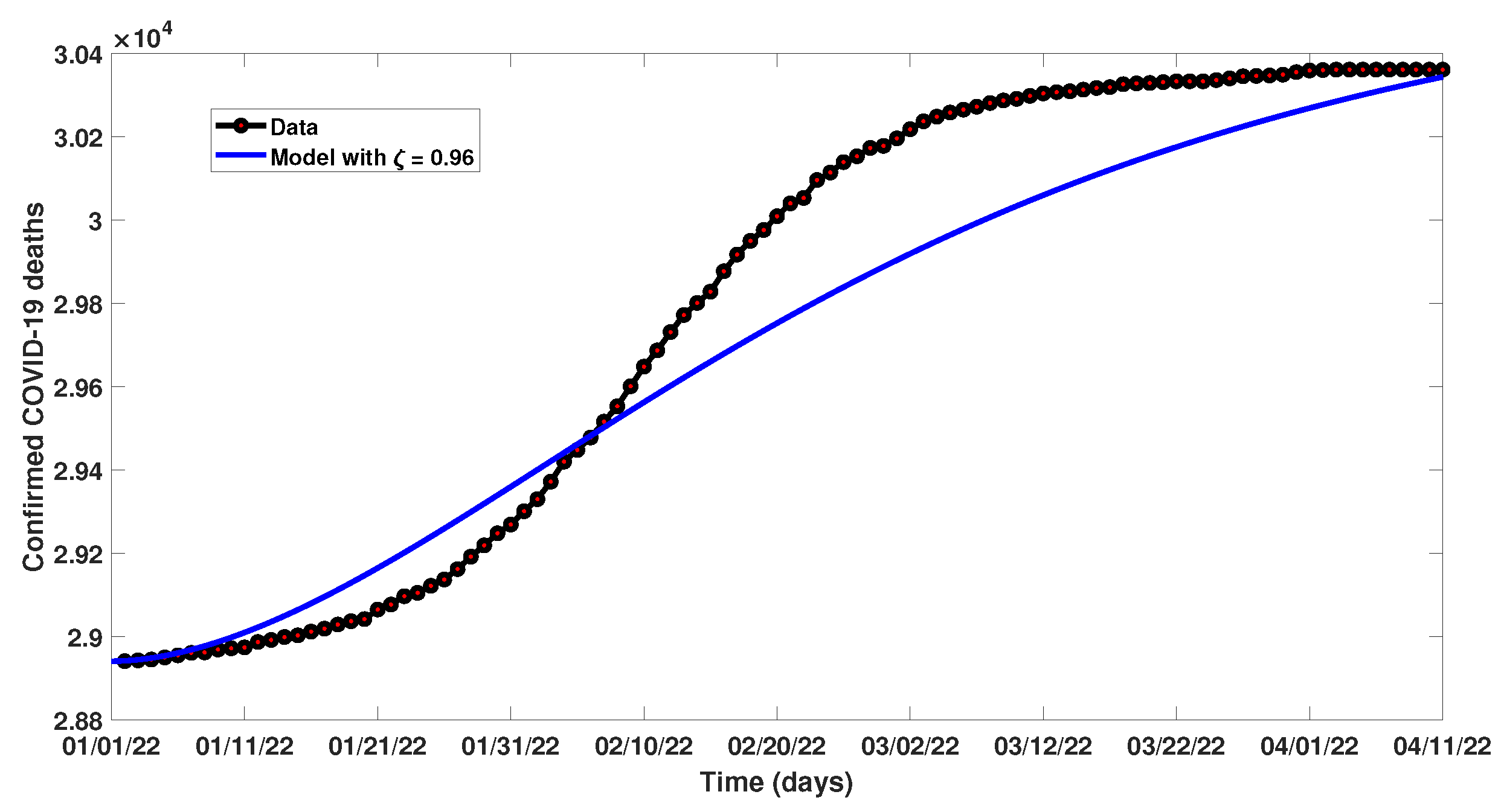
Using the data available for the daily confirmed COVID-19 deaths in Pakistan [33] between 1 January 2022 and 10 April 2022, the fractional model is fitted to the data. During this period, both the Delta and Omicron variants were in high circulation within Pakistan. Parameter values estimated from the fitting are shown in Table 1. The fitting shown in Figure 2 reveals that our model fits very well to the data when the fractional order $\zeta =0.96$.

6.3. Numerical Assessment

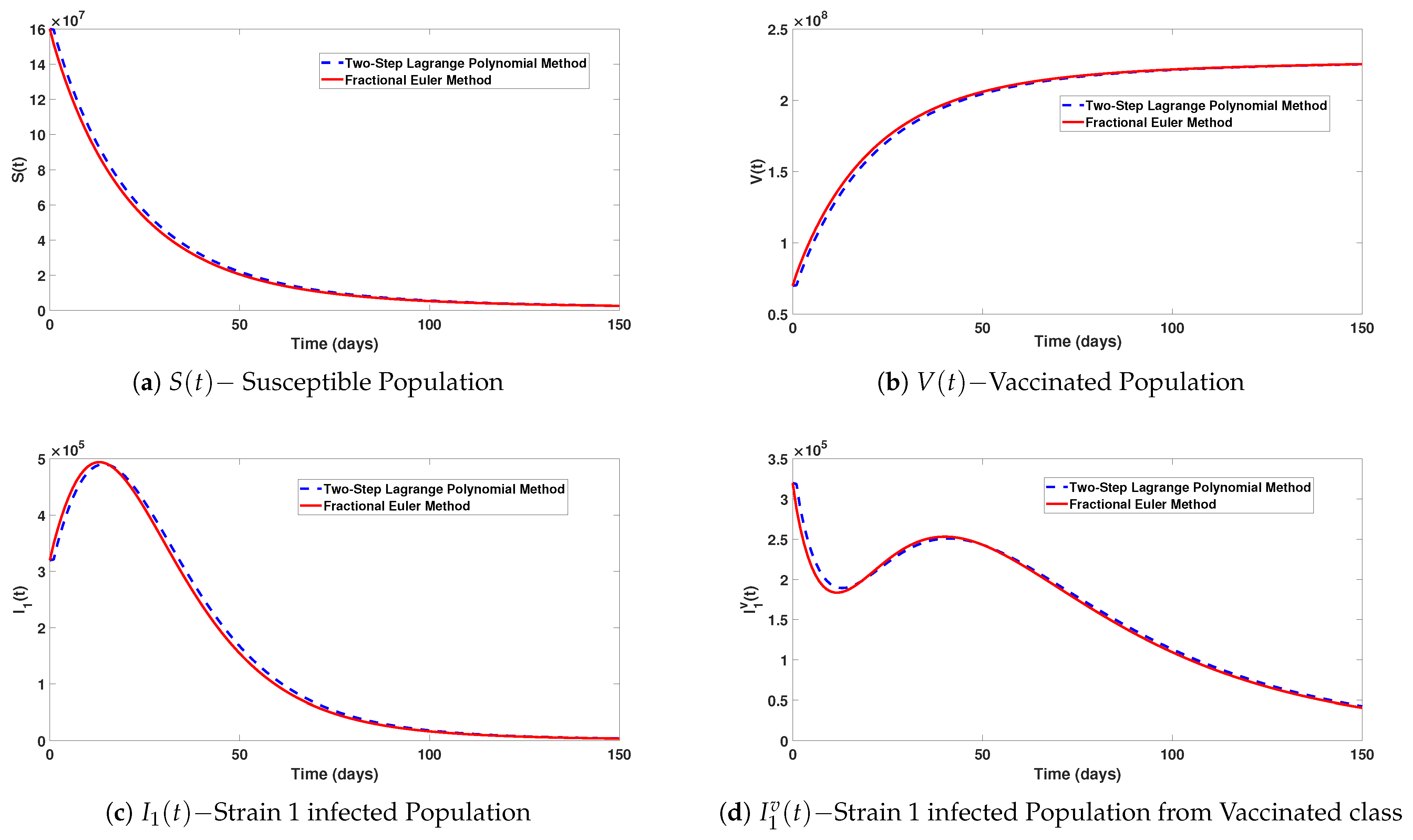
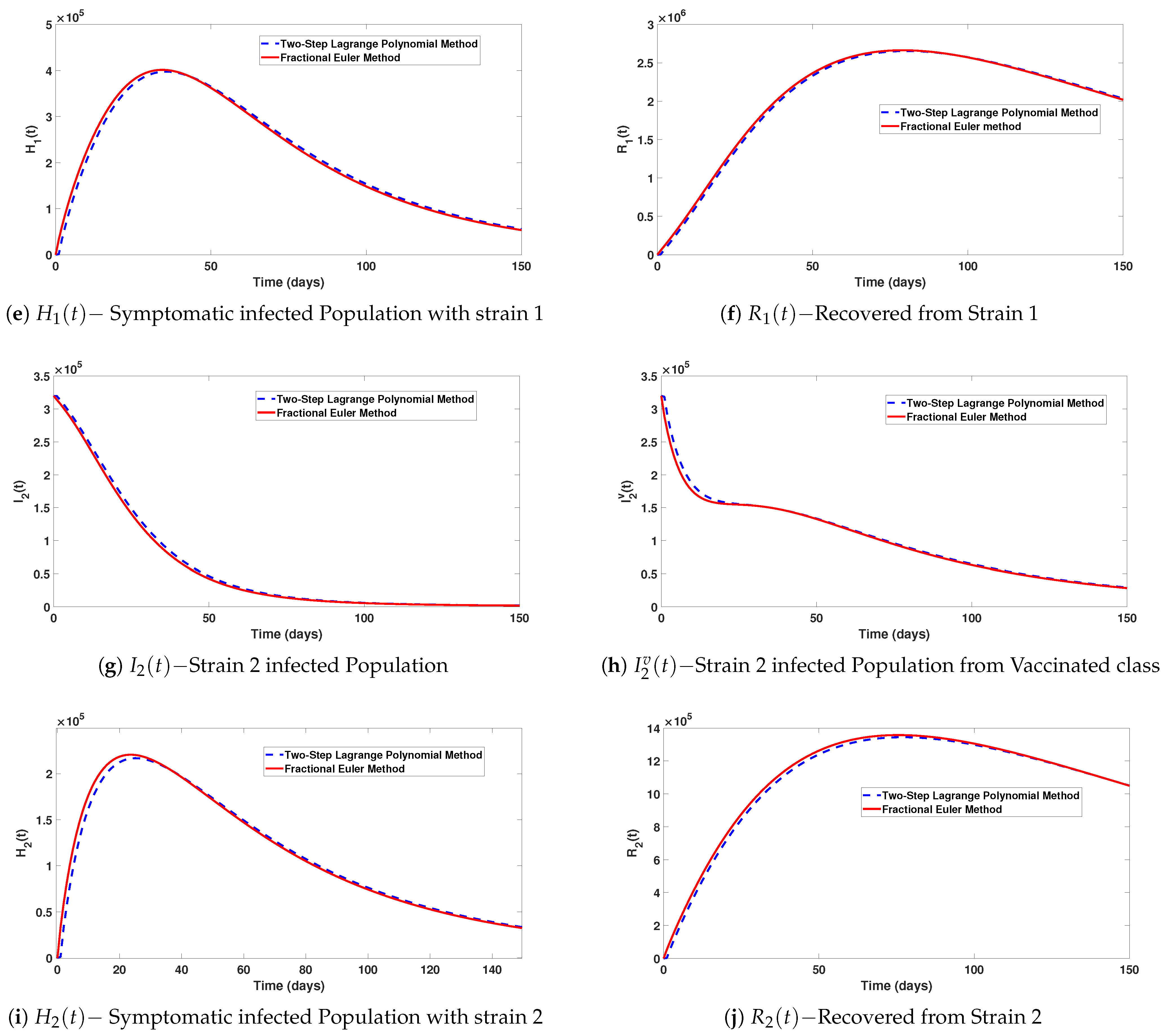
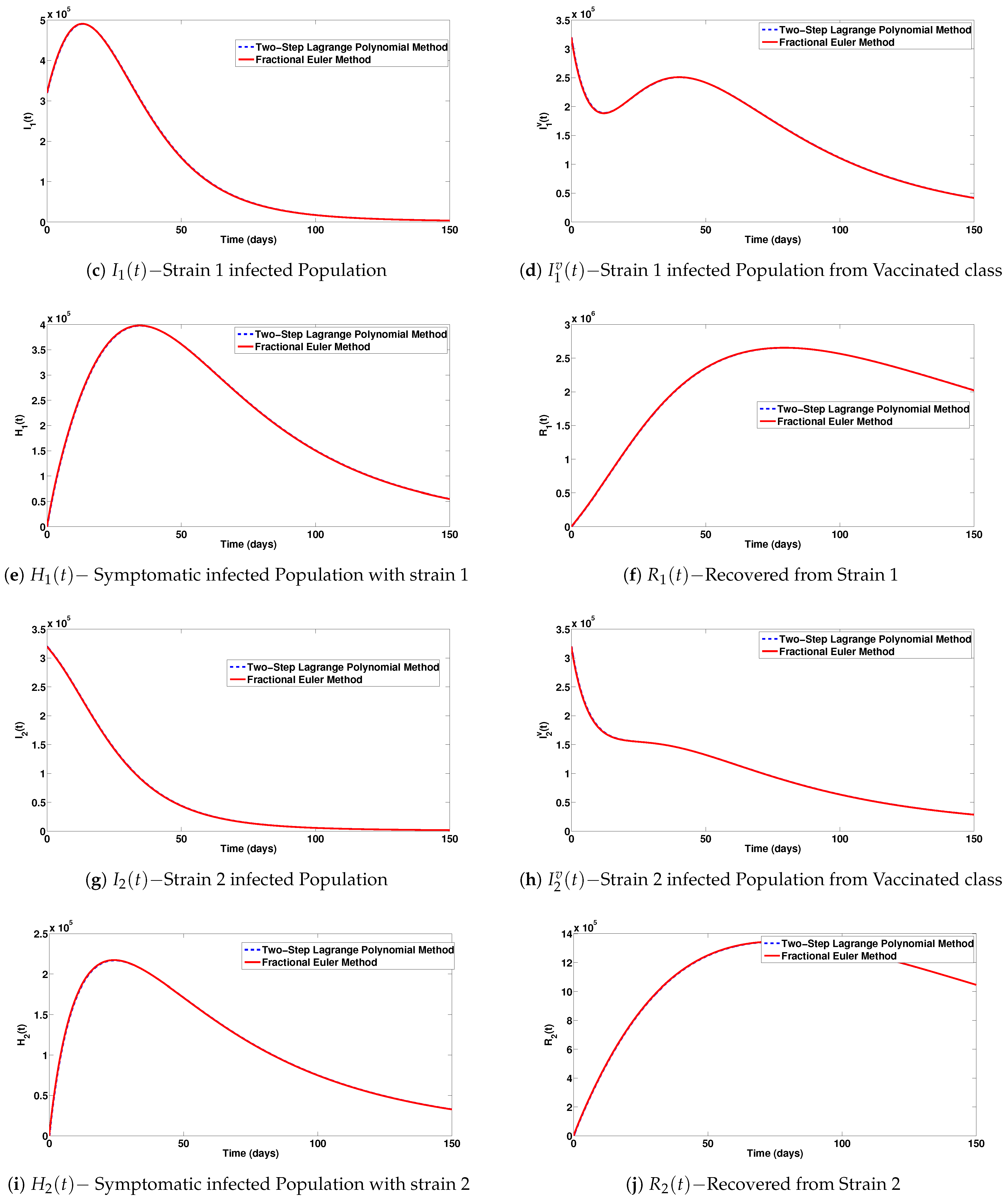
In Figure 3a–j, simulations of the various classes comparing the two-step Lagrange polynomial method and the fractional Euler method are presented. We take the fractional order equal to $\zeta =0.96$ and the step size $h=1.0$. It is observed that the behaviours of both methods are close, but not the same. However, by decreasing the step size h to $0.1$, as shown in Figure 4a–j, both methods behave well and almost the same.

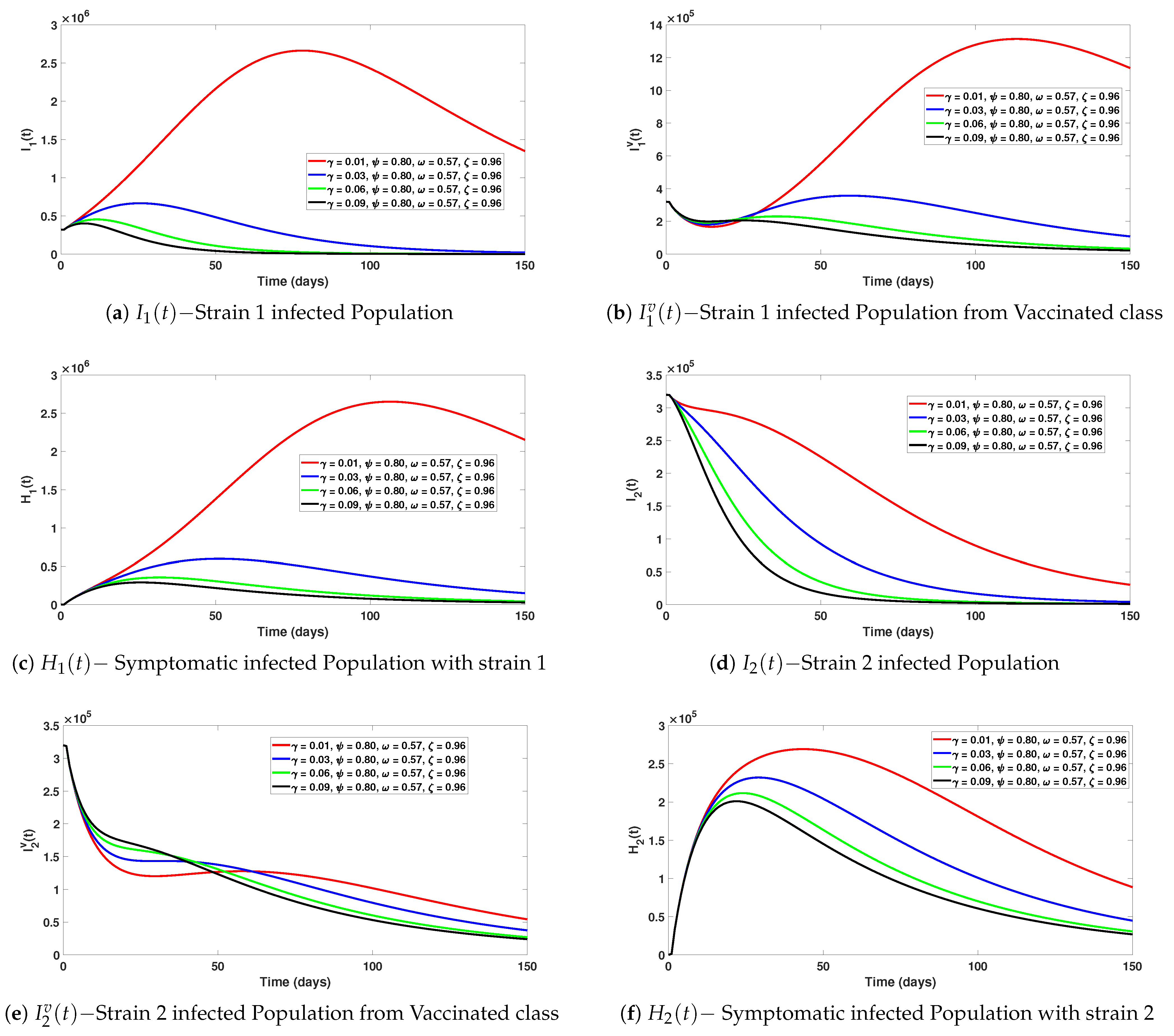
In Figure 5a–f, simulations of the various classes of System (1) assessing the impact of vaccination are highlighted using the two-step Lagrange polynomial method, where the fractional order is $\zeta =0.90$ and the step size $h=0.1$. In particular, it is observed that increasing the vaccination rate $\gamma$ from $0.01$ to $0.09$ decreases the number of people infected with the Omicron SARS-CoV-2 variant, as can be seen in Figure 5a–c. Additionally, a noticeable decrease is observed in the total number of infected individuals with the Delta SARS-CoV-2 variant, as can be seen in Figure 5d–f. This is due to the high efficacy of the vaccine against both variants. Thus, a safe and effective vaccination program is crucial for the elimination of the different variants of concern.

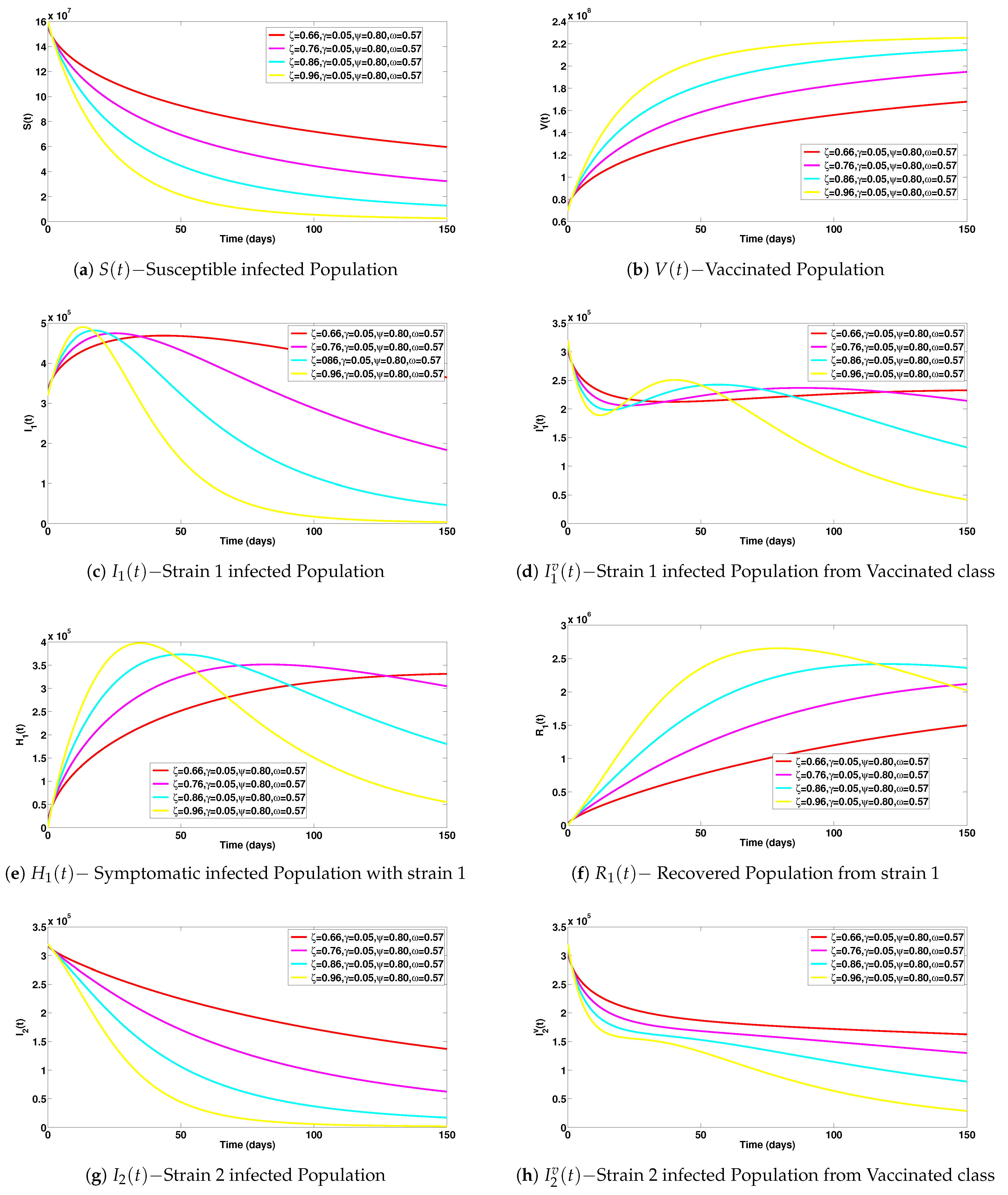
Numerical experiments on System (1) for various fractional orders are presented in Figure 6a–j. The impact of the fractional orders are clearly observed.

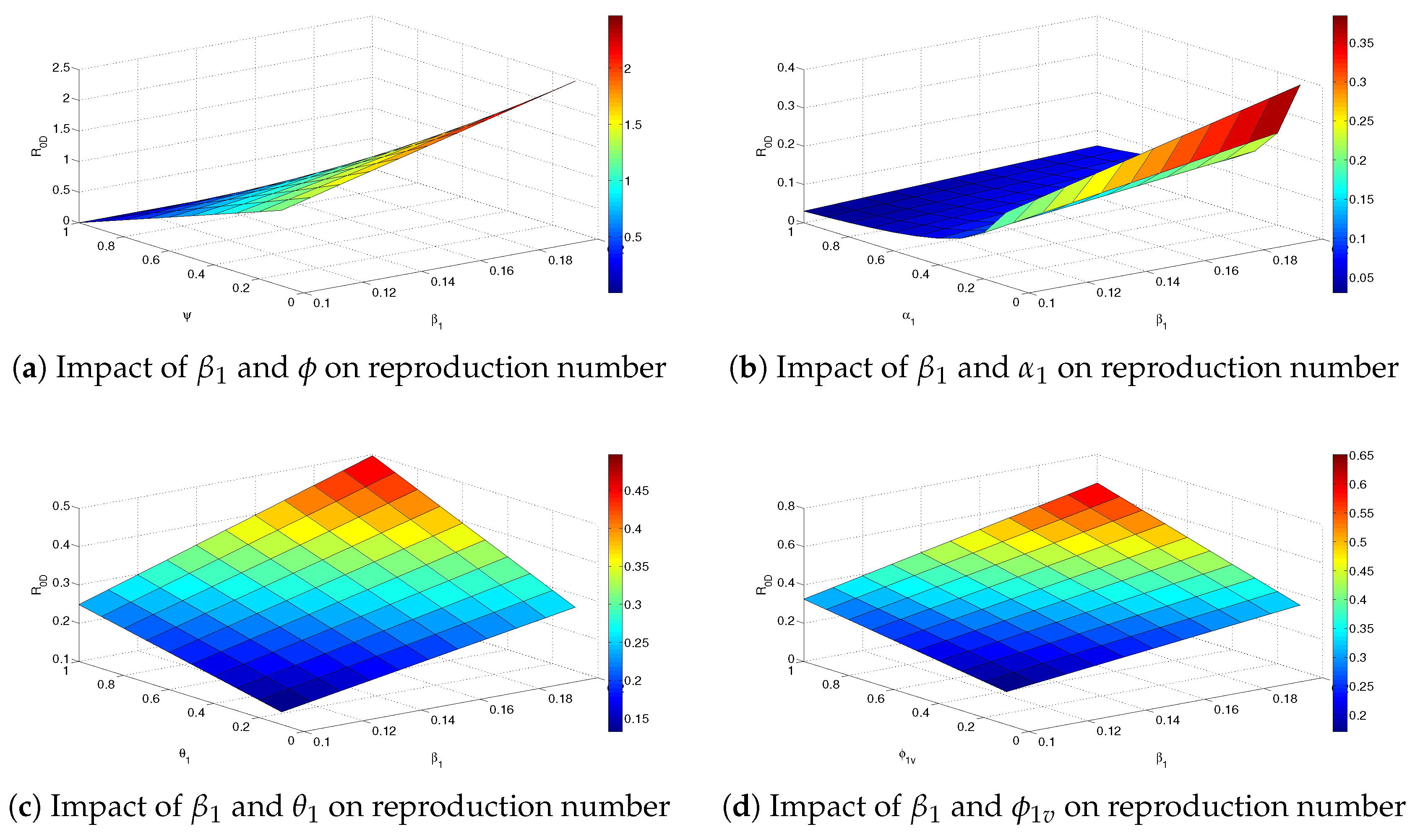
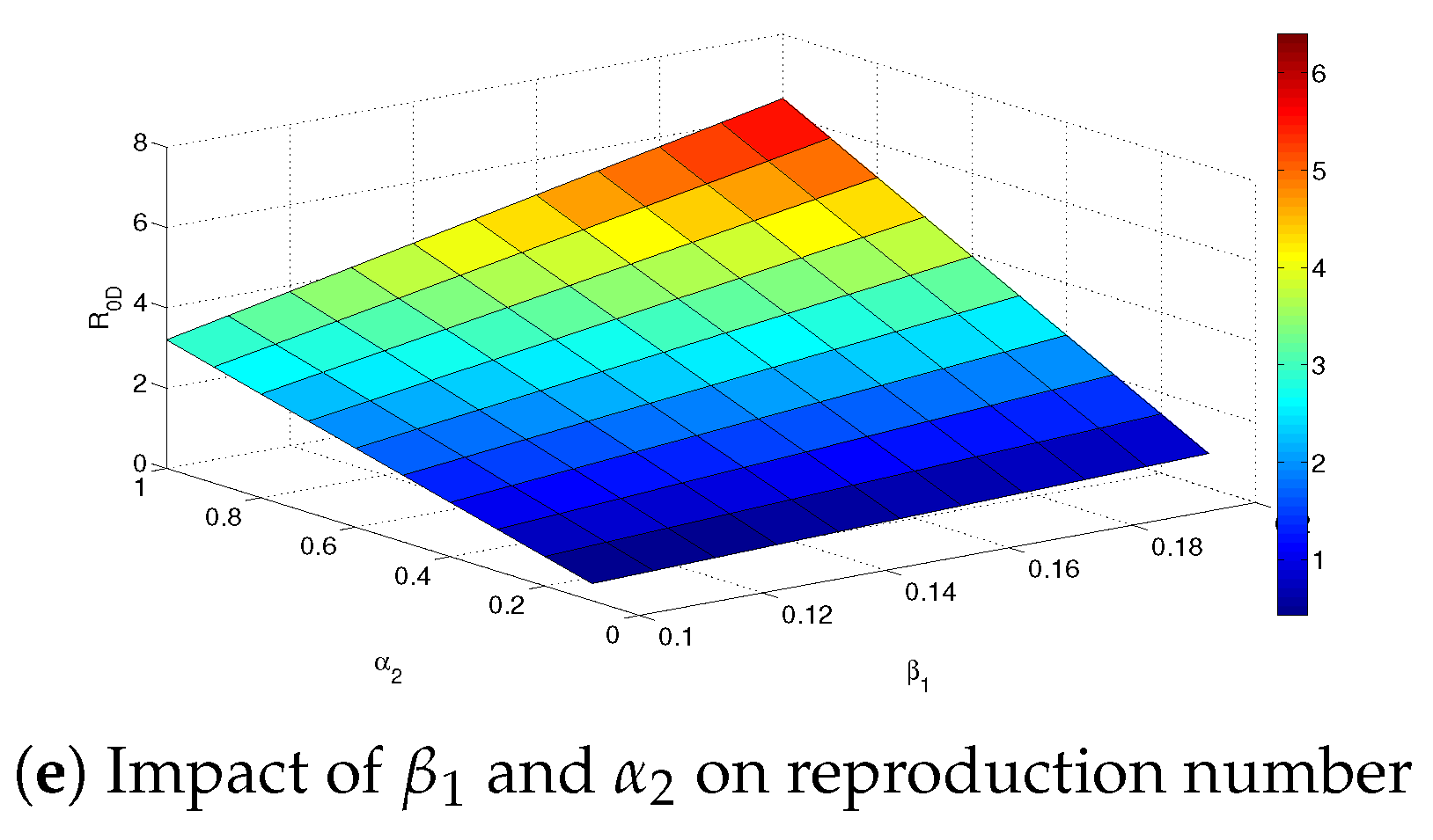
Numerical assessments of the impact of various parameters on the Delta variant’s reproduction number are presented in Figure 7a–e. Specifically, Figure 7a depicts the surface plot of the Delta variant’s reproduction number as a function of the transmission rate (${\beta }_1$) and vaccine efficacy ($\psi$). It is observed in this figure that, as the transmission rate is increased, the reproduction number and disease burden also increase. However, it is noted that increased vaccine efficacy decreases both the reproduction number and disease burden.

In Figure 7b, the surface plot of the Delta variant’s reproduction number as a function of transmission rate ${\beta }_1$ and progression rate ${\alpha }_1$ is presented. It can be seen from this figure that as the transmission and progression rates increase, the reproduction number also increases.

In Figure 7c, a surface plot of the reproduction number for the Delta variant as a function of the transmission rates ${\beta }_1$ and ${\theta }_1$ is presented. It can be observed that as the transmission rate and modification parameters accounting for the infectivity of symptomatic individuals increase, the reproduction number and disease burden also increases. A similar conclusion can be drawn for the surface plots presented in Figure 7d,e.

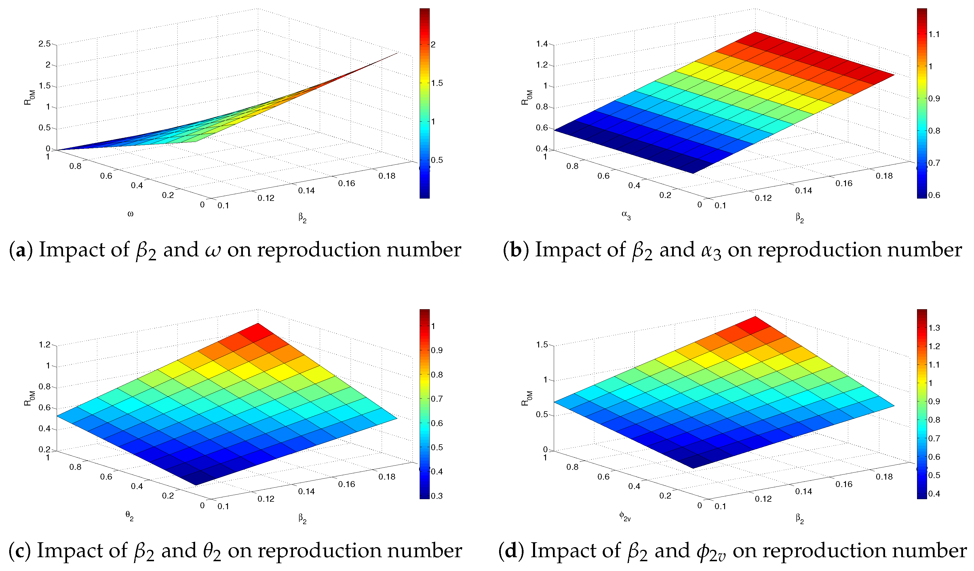
Numerical experiments to assess the impact of various parameters on the Omicron variant’s reproduction number are presented in Figure 8a–e. For instance, in Figure 8a, the surface plot for the Omicron variant’s reproduction number as a function of the transmission rate (${\beta }_2$) and vaccine efficacy ($\omega$) is presented. It is observed that as the transmission rate increases, the reproduction number and disease burden also increase. However, it is noted that as the vaccine efficacy increases, the reproduction number decreases. This shows that to reduce disease burden, the vaccine efficacy must be as high as possible.

In Figure 8b, a surface plot of the Omicron variant’s reproduction number as a function of the transmission rate ${\beta }_2$ and progression rate ${\alpha }_3$ is presented. From the plot, it can be noted that, as the transmission rate and progression rates increase, both the reproduction number and the disease burden increase.

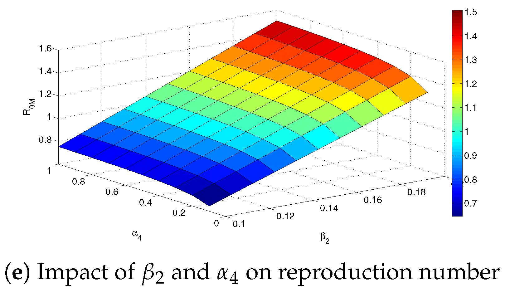
In Figure 8c, a surface plot of the Omicron variant’s reproduction number as a function of the transmission rate ${\beta }_2$ and modification parameter ${\theta }_2$ is presented. From this figure, it can be observed that, as the transmission rate and the modification parameter accounting for the infectivity of individuals in the symptomatic class are increased, the reproduction number also increases. Similar conclusions can be made for the surface plots presented in Figure 8d,e.

7. Conclusions

In this paper, a new vaccination model for SARS-CoV-2 variants was developed and analyzed. The model assumes variability in transmission rates due to vaccination, where the asymptomatic infected classes were categorized based on their vaccination history. Using the Banach contraction principle and the Arzela–Ascoli theorem, the existence and uniqueness results for the fractional system were obtained. Two numerical schemes, the two-step Lagrange polynomial and the fractional Euler methods, were employed to discuss the approximate solution of the system. The model was fitted to data associated with COVID-19 deaths in Pakistan between 1 January 2022 and 10 April 2022. Assessing the fractional system numerically, the impact of vaccination and fractional order were highlighted, where it was observed that vaccination could remarkably curtail the spikes of emerging variants of SARS-CoV-2 within the population.

Important highlights from the qualitative analysis are:

(i).

The proposed fractional-order system was shown to be positively invariant using Theorem 1.

(ii).

Conditions for the existence of a solution to the fractional-order system were obtained using Theorems 2 and 3, while the uniqueness result was presented using Theorem 4.

(iii).

The designed model was also shown to be generalized Ulam–Hyers stable with the help of Theorem 6.

Highlights of the simulations include:

(iv).

The proposed model fits well to data when the order of the fractional derivative is taken as $\zeta =0.96$, as can be observed in Figure 2.

(v).

The two numerical approaches were thus compared with different step sizes, where it was concluded that they behave closely for very small step sizes and differently for larger step sizes, as can be observed in Figure 3 and Figure 4.

(vi).

It was observed that increasing the vaccination rate $\gamma$ from $0.01$ to $0.09$ caused a significant decrease in the number of people infected with the Omicron SARS-CoV-2 variant, as can be seen in Figure 5a–c.

(vii).

Surface plots showing the important parameters driving the dynamics of the disease are presented in Figure 7 and Figure 8.

The model discussed in this study has some limitations. The model did not capture any interaction between the variants. Thus, future work in this direction may consider infection-acquired cross-immunity, cross-enhancement, super-infection, and dual co-infection with both variants. One could also study the in-host dynamics between both variants of SARS-CoV-2. In addition, one could also consider stochastic equivalence of the current model for a possible research problem. Moreover, one could also establish existence, uniqueness, and stability results using some novel fixed-point theorems.

References

1. Hu, B.; Guo, H.; Zhou, P.; Shi, Z.L. Characteristics of SARS-CoV-2 and COVID-19. Nat. Rev. Microbiol. 2021, 19, 141–154. [Google Scholar] [CrossRef]
2. United States Food and Drug Administration. FDA Takes Key Action in Fight Against COVID-19 By Issuing Emergency Use Authorization for First COVID-19 Vaccine. 2020. Available online: https://www.fda.gov/news-events/press-announcements/fda-takes-key-action-fight-against-covid-19-issuing-emergency-use-authorization-first-covid-19 (accessed on 17 June 2021).
3. Interim Clinical Considerations for Use of COVID-19 Vaccines Currently Authorized in the United States. Available online: https://www.cdc.gov/vaccines/covid-19/clinical-considerations/covid-19-vaccines-us.html (accessed on 14 July 2021).
4. Tang, P.; Hasan, M.R.; Chemaitelly, H.; Yassine, H.M.; Benslimane, F.M.; Al Khatib, H.A.; AlMukdad, S.; Coyle, P.; Ayoub, H.H.; Al Kanaani, Z.; et al. BNT162b2 and mRNA-1273 COVID-19 vaccine effectiveness against the SARS-CoV-2 Delta variant in Qatar. Nat. Med. 2021; Epub ahead of print. [Google Scholar] [CrossRef]
5. Andrews, N.; Tessier, E.; Stowe, J.; Gower, C.; Kirsebom, F.; Simmons, R.; Gallagher, E.; Chand, M.; Brown, K.; Ladhani, S.N.; et al. Vaccine effectiveness and duration of protection of Comirnaty, Vaxzevria and Spikevax against mild and severe COVID-19 in the UK. medRxiv 2021. [Google Scholar] [CrossRef]
6. Nasreen, S.; Chung, H.; He, S.; Brown, K.A.; Gubbay, J.B.; Buchan, S.A.; Fell, D.B.; Austin, P.C.; Schwartz, K.L.; Sundaram, M.E.; et al. Effectiveness of COVID-19 vaccines against symptomatic SARS-CoV-2 infection and severe outcomes with variants of concern in Ontario. Nat. Microbiol. 2022, 7, 379–385. [Google Scholar] [CrossRef] [PubMed]
7. Puranik, A.; Lenehan, P.J.; Silvert, E.; Niesen, M.J.M.; Corchado-Garcia, J.; O’Horo, J.C.; Virk, A.; Swift, M.D.; Halamka, J.; Badley, A.D.; et al. Comparison of two highly-effective mRNA vaccines for COVID-19 during periods of Alpha and Delta variant prevalence. medRxiv 2021. [Google Scholar] [CrossRef]
8. Nanduri, S.; Pilishvili, T.; Derado, G.; Soe, M.M.; Dollard, P.; Wu, H.; Li, Q.; Bagchi, S.; Dubendris, H.; Link-Gelles, R.; et al. Effectiveness of Pfizer-BioNTech and Moderna Vaccines in Preventing SARS-CoV-2 Infection Among Nursing Home Residents Before and During Widespread Circulation of the SARS-CoV-2 B.1.617.2 (Delta) Variant— National Healthcare Safety Network, March 1–August 1, 2021. Morb. Mortal. Wkly Rep. 2021, 70, 1163–1166. [Google Scholar]
9. Fowlkes, A.; Gaglani, M.; Groover, K.; Thiese, M.S.; Tyner, H.; Ellingson, K. Effectiveness of COVID-19 Vaccines in Preventing SARS-CoV-2 Infection Among Frontline Workers Before and During B.1.617.2 (Delta) Variant Predominance—Eight U.S. Locations, December 2020–August 2021. Morb. Mortal. Wkly Rep. 2021, 70, 1167–1169. [Google Scholar] [CrossRef]
10. Israel Ministry of Health. COVID-19 Vaccine Effectiveness against the Delta Variant. Israel’s Ministry of Health Report. 2021. Available online: Https://www.gov.il/BlobFolder/reports/vaccine-efficacy-safety-follow-up-committee/he/files_publications_corona_two-dose-vaccination-data.pdf (accessed on 11 November 2022).
11. Ali, A.; Khan, S.U.; Ali, I.; Khan, F.U. On dynamics of stochastic avian influenza model with asymptomatic carrier using spectral method. Math. Methods Appl. Sci. 2022, 45, 8230–8246. [Google Scholar] [CrossRef]
12. Bonyah, E.; Khan, M.A.; Okosun, K.O.; Gómez-Aguilar, J.F. On the co-infection of dengue fever and Zika virus. Optim. Contr. Appl. Meth. 2019, 40, 394–421. [Google Scholar] [CrossRef]
13. Rihan, F.A.; Alsakaji, H.J. Dynamics of a stochastic delay differential model for COVID-19 infection with asymptomatic infected and interacting people: Case study in the UAE. Results Phys. 2021, 28, 104658. [Google Scholar] [CrossRef]
14. Rihan, F.A.; Alsakaji, H.J.; Rajivganthi, C. Stochastic SIRC epidemic model with time-delay for COVID-19. Adv. Differ. Equ. 2020, 2020, 502. [Google Scholar] [CrossRef]
15. Omame, A.; Abbas, M. Modeling SARS-CoV-2 and HBV co-dynamics with optimal control. Physica A 2023, 615, 128607. [Google Scholar] [CrossRef] [PubMed]
16. Omame, A.; Abbas, M. The stability analysis of a co-circulation model for COVID-19, dengue, and zika with nonlinear incidence rates and vaccination strategies. Healthc. Anal. 2023, 3, 100151. [Google Scholar] [CrossRef] [PubMed]
17. Metzler, R.; Klafter, J. The random walk’s guide to anomalous diffusion: A fractional dynamics approach. Phys. Rep. 2000, 339, 1–77. [Google Scholar] [CrossRef]
18. Kilbas, A.A.; Srivastava, H.M.; Trujillo, J.J. Theory and Applications of Fractional Differential Equations; North-Holland Mathematics Studies; Elsevier Science: Amsterdam, The Netherlands, 2006; p. 204. [Google Scholar]
19. Lin, W. Global existence theory and chaos control of fractional differential equations. J. Math. Anal. Appl. 2007, 332, 709–726. [Google Scholar] [CrossRef]
20. Caputo, M.; Fabrizio, M. A new definition of fractional derivative without singular kernel. Prog. Fract. Differ. Appl. 2015, 1, 73–85. [Google Scholar]
21. Atangana, A.; Baleanu, D. New fractional derivatives with nonlocal and non-singular kernel: Theory and applications to heat transfer model. Therm Sci. 2016, 20, 763–769. [Google Scholar] [CrossRef]
22. Omame, A.; Abbas, M.; Onyenegecha, C.P. A fractional-order model for COVID-19 and tuberculosis co-infection using Atangana-Baleanu derivative. Chaos Solitons Fractals 2021, 153, 111486. [Google Scholar] [CrossRef]
23. Omame, A.; Abbas, M.; Nwajeri, U.K. A fractional-order control model for Diabetes COVID-19 co-dynamics with Mittag-Leffler function. Alex. Eng. J. 2022, 61, 7619–7635. [Google Scholar] [CrossRef]
24. Ogunrinde, R.B.; Nwajeri, U.K.; Fadugba, S.E.; Ogunrinde, R.R.; Oshinubi, K.I. Dynamic model of COVID-19 and citizens reaction using fractional derivative. Alex. Eng. J. 2021, 60, 2001–2012. [Google Scholar] [CrossRef]
25. Asamoah, J.K.K. Fractal-fractional model and numerical scheme based on Newton polynomial for Q fever disease under Atangana-Baleanu derivative. Results Phys. 2022, 34, 105189. [Google Scholar] [CrossRef]
26. Asamoah, J.K.K.; Okyere, E.; Yankson, E.; Opoku, A.A.; Adom-Konadu, A.; Acheampong, E.; Arthur, Y.D. Non-fractional and fractional mathematical analysis and simulations for Q fever. Chaos Solitons Fractals 2022, 156, 111821. [Google Scholar] [CrossRef]
27. Safari, F.; Chen, W. Numerical approximations for space-time fractional Burgers equations via a new semi-analytical method. Comput. Math. Appl. 2021, 96, 55–66. [Google Scholar] [CrossRef]
28. Jafari, H.; Khalique, C.M.; Nazari, M. Application of the Laplace decomposition method for solving linear and nonlinear fractional diffusion-wave equations. Appl. Math. Lett. 2011, 24, 1799–1805. [Google Scholar] [CrossRef]
29. Omame, A.; Zaman, F.D. Solution of the modified time fractional coupled Burgers equation using Laplace Adomian decomposition method. Acta Mech. Autom. 2023, 17, 124–132. [Google Scholar] [CrossRef]
30. Podlubny, I. Fractional Differential Equations; Academic Press: San Diego, CA, USA, 1999. [Google Scholar]
31. Rothana, H.A.; Byrareddy, S.N. The epidemiology and pathogenesis of coronavirus disease (COVID-19) outbreak. J. Autoimmun. 2020, 109, 102433. [Google Scholar] [CrossRef] [PubMed]
32. Chen, T.-M.; Rui, J.; Wang, Q.-P.; Zhao, Z.-Y.; Cui, J.-A.; Yin, L. A mathematical model for simulating the phase-based transmissibility of a novel coronavirus. Infect. Dis. Poverty 2020, 9, 24. [Google Scholar] [CrossRef]
33. Pakistan: Coronavirus Pandemic Country Profile. Available online: https://ourworldindata.org/coronavirus/country/pakistan (accessed on 11 November 2022).
34. Yong, Z.; Jinrong, W.; Lu, Z. Basic Theory of Fractional Differential Equations; World Scientific: Singapore, 2016. [Google Scholar]
35. van den Driessche, P.; Watmough, J. Reproduction numbers and sub-threshold endemic equilibria for compartmental models of disease transmission. Math. Biosci. 2002, 180, 29–48. [Google Scholar] [CrossRef] [PubMed]
36. Ulam, S.M. A Collection of Mathematical Problems; Interscience Publishers: New York, NY, USA, 1960. [Google Scholar]
37. Ulam, S.M. Problem in Modern Mathematics; Dover Publications: Mineola, NY, USA, 2004. [Google Scholar]
38. Toufik, M.; Atangana, A. New numerical approximation of fractional derivative with non-local and non-singular kernel: Application to chaotic models. Eur. Phys. J. Plus 2017, 132, 444. [Google Scholar] [CrossRef]
39. Li, C.; Zeng, F. The finite difference methods for fractional ordinary differential equations. Numer. Funct. Anal. Optim. 2013, 34, 149–179. [Google Scholar] [CrossRef]
40. Diethelm, K.; Ford, N.J.; Freed, A.D. Detailed error analysis for a fractional Adams method. Numer. Algorithms 2004, 36, 31–52. [Google Scholar] [CrossRef]
41. Baleanu, D.; Jajarmi, A.; Hajipour, M. On the nonlinear dynamical systems within the generalized fractional derivatives with Mittag-Leffler kernel. Nonlinear Dyn. 2018, 94, 397–414. [Google Scholar] [CrossRef]
Figure 1. Schematic diagram of Model (1), with λ 1 = β 1 ( I 1 + ϕ 1 v I 1 v + θ 1 H 1 ) N , λ 2 = β 2 ( I 2 + ϕ 2 v I 2 v + θ 2 H 2 ) N .
Axioms 12 00480 g001
Figure 2. Fitting the model to data.
Axioms 12 00480 g002
Figure 3. Simulations of the various classes comparing the two-step Lagrange polynomial method and the fractional Euler method. Here, the fractional order is ζ = 0.96 , and the step size h = 1.0 .
Axioms 12 00480 g003aAxioms 12 00480 g003b
Figure 4. Simulations of the various classes comparing the two-step Lagrange polynomial method and the fractional Euler method. Here, the fractional order is ζ = 0.96 , and the step size h = 0.1 .
Axioms 12 00480 g004aAxioms 12 00480 g004b
Figure 5. Simulations of the various classes of System (1) assessing the impact of vaccination using the two-step Lagrange polynomial method. Here, the fractional order is ζ = 0.96 , and the step size h = 0.1 .
Axioms 12 00480 g005
Figure 6. Simulations of the various classes of System (1) assessing the impact of fractional order using the two-step Lagrange polynomial method. Here, the step size h = 0.1 .
Axioms 12 00480 g006aAxioms 12 00480 g006b
Figure 7. Simulations of the reproduction number for Delta variant for System (1) assessing the impact of different parameters.
Axioms 12 00480 g007aAxioms 12 00480 g007b
Figure 8. Simulations of the reproduction number for Omicron variant for System (1) assessing the impact of different parameters.
Axioms 12 00480 g008aAxioms 12 00480 g008b