The Markov Bernoulli Lomax with Applications Censored and COVID-19 Drought Mortality Rate Data

Abstract

In this article, we present a Markov Bernoulli Lomax (MB-L) model, which is obtained by a countable mixture of Markov Bernoulli and Lomax distributions, with decreasing and unimodal hazard rate function (HRF). The new model contains Marshall- Olkin Lomax and Lomax distributions as a special case. The mathematical properties, as behavior of probability density function (PDF), HRF, r^th moments, moment generating function (MGF) and minimum (maximum) Markov-Bernoulli Geometric (MBG) stable are studied. Moreover, the estimates of the model parameters by maximum likelihood are obtained. The maximum likelihood estimation (MLE), bias and mean squared error (MSE) of MB-L parameters are inspected by simulation study. Finally, a MB-L distribution was fitted to the randomly censored and COVID-19 (complete) data.

1. Introduction

The emergence of modern applications and many developments in various fields, in addition to the limitations of some well-known distributions, lead us to create other distributions that are more suitable for modern applications and free from restrictions.

Gharib et al. [1] used a countable mixture with a Markov Bernoulli geometric model to introduced a new family, which its survival function (SF) is given by:

$$\overline{G}\left(x,\alpha ,\rho \right)=\frac{\alpha \overline{F}\left(x\right)\left[1-\rho \overline{F}\left(x\right)\right]}{1-\left[1-\left(1-\rho \right)\alpha \right]\overline{F}\left(x\right)},\left(x\in ℝ, \alpha >0, 0\le \rho <1\right)$$

(1)

When $\rho =0$, the SF $\overline{G}\left(x,\alpha ,\rho \right)$ in (1) reduces to the SF $\overline{G}\left(x,\alpha \right)$ which is introduced by Marshall and Olkin [2]. Moreover, if, $\rho =1-\frac{1}{\alpha }$ then $\overline{G}\left(x,\alpha ,\rho \right)$ in (1) reduces to:

$$\overline{G}\left(x,\alpha \right)=\overline{F}\left(x\right)\left[\alpha F\left(x\right)+\overline{F}\left(x\right)\right].\left(x\in ℝ, \alpha >1\right)$$

(2)

For $\rho =0$ and α = 1 the SF $\overline{G}\left(x,\alpha ,\rho \right)$ reduces to $\overline{F}\left(x\right)$.

The SF of Lomax or (Pareto Type-II) distribution is:

$$\overline{F}\left(x\right)={(1+\beta x)}^{-\theta },\hspace{1em}x>0,\beta ,\theta >0.$$

The probability density function (PDF) and hazard rate function (HRF) are:

$$f\left(x\right)={\beta \theta \left(1+\beta x\right)}^{-\theta -1},$$

$$h_F\left(r\right)={\beta \theta \left(1+\beta x\right)}^{-1}.$$

Johnson et al. [3] used the Lomax model in practical and theoretical fields as, economics and biological. Moreover, Harris [4], Bryson [5], Cordeiro et al. [6] and Bhagwati Devi [7] are, respectively, used this model in reliability & life testing, income and wealth data, firm size data and Entropy.

In the past few years, several authors have expanded the Lomax distribution due to its importance in life time distributions as: generalized Lomax (Raj Kamal Maurya et al. [8]), Poisson-Lomax (Mohammed et al. [9]), Marshall–Olkin Power Lomax (Muhammad Ahsanul Haq et al. [10]), the type II Topp Leone-Power Lomax (Sirinapa Aryuyuen and Winai Bodhisuwan [11]), new weighted Lomax (Huda M. Alshanbari et al. [12]) and reflected-shifted-truncated Lomax Distribution (Sanku Dey et al. [13]), there are other generalizations of the Lomax distribution, and they different in terms of the form of the PDF and the behavior of the HRF; see, Ghitany et al. [14], Lemonte and Cordeiro [15], Cordeiro et al. [16], Al-Zahrani and Sagor [17,18], Tahir et al. [19], El-Bassiouny et al. [20], Rady et al. [21] and Cooray et al. [22], Wael S. Abu El Azm et al. [23], Hassan Alsuhabi et al. [24] and Adebisi A. Ogunde [25].

If we put $\overline{F}\left(x\right)={(1+\beta x)}^{-\theta },x>0,\beta ,\theta >0$, which is the SF of the Lomax distribution, in (1), we have the MB-L (α, β, θ, $\rho$) model is:

$$\overline{G}\left(x,\alpha ,\beta ,\theta ,\rho \right)=\frac{\alpha {(1+\beta x)}^{-\theta }\left[1-\rho {(1+\beta x)}^{-\theta }\right]}{1-\left[1-\left(1-\rho \right)\alpha \right]{(1+\beta x)}^{-\theta }},\hspace{1em}x>0, \alpha ,\lambda >0, 0\le \rho <1$$

(3)

2. The PDF of the MB-L Model

From Equation (3), we have:

$$\begin{gathered} g\left(x\right)=\frac{\alpha \beta {\left(1+x\beta \right)}^{-1-\theta }\theta \left({\left(1+x\beta \right)}^{2\theta }-\left(-1+\alpha +2{\left(1+x\beta \right)}^{\theta }\right)\rho +\alpha {\rho }^2\right)}{{\left(-1+\alpha +{\left(1+x\beta \right)}^{\theta }-\alpha \rho \right)}^2}, \\ x>0,\alpha >0,\lambda >0,0\le \rho <1 \end{gathered}$$

(4)

When α = 0, $\overline{G}\left(x,\alpha ,\beta ,\theta ,\rho \right)$ and $g\left(x\right)$, reduce to corresponding the MOEL distribution Ghitany et al. [14].

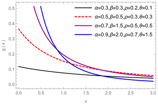
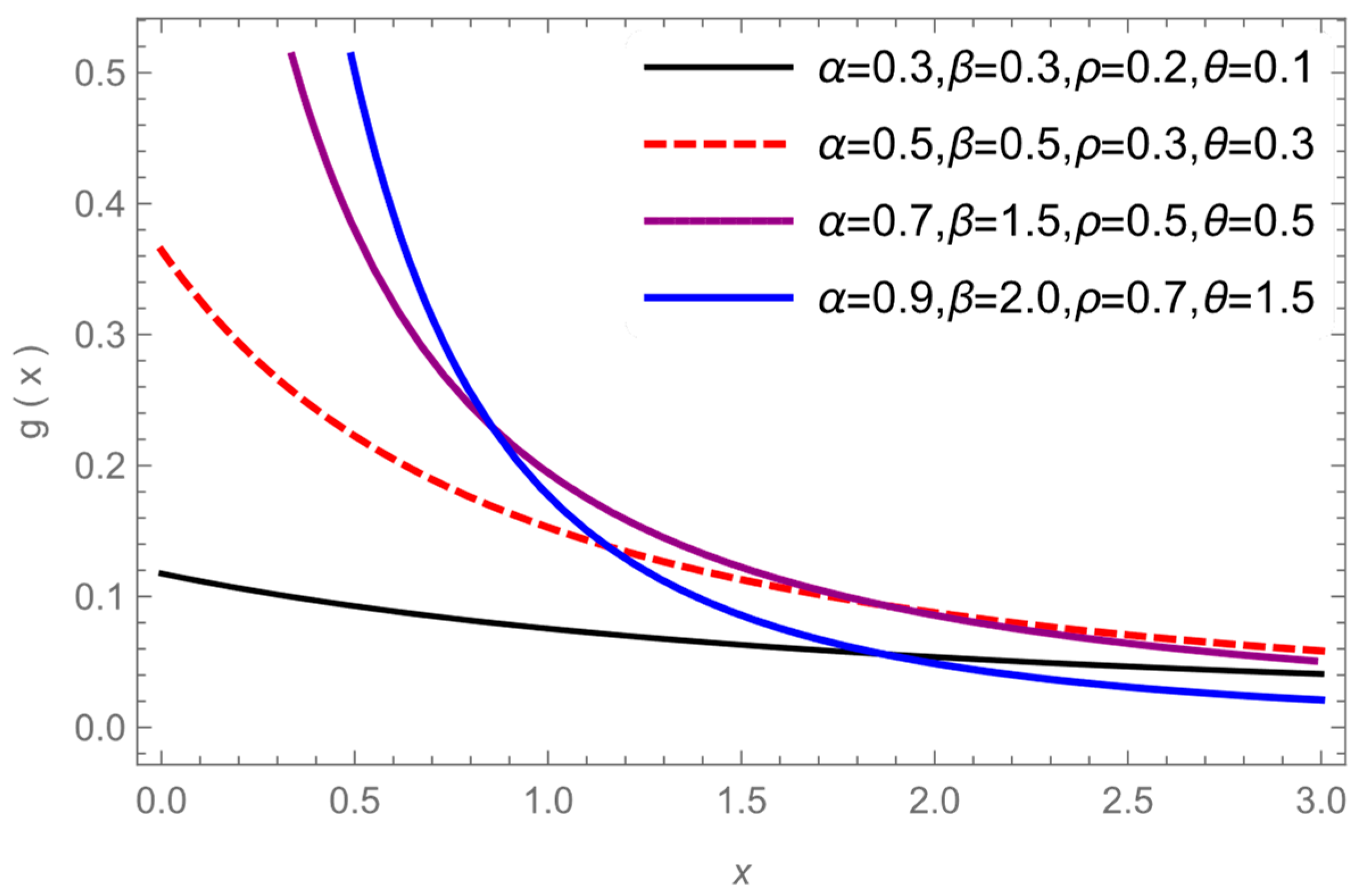
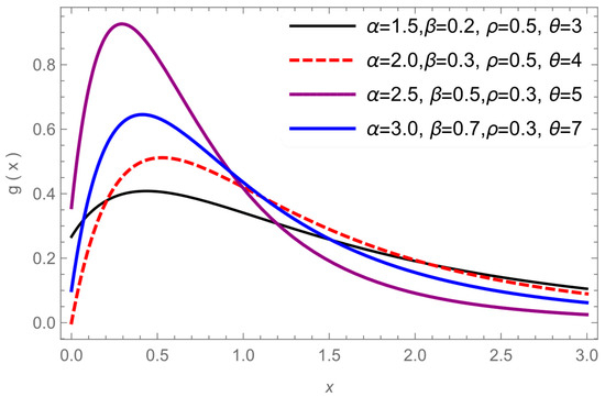
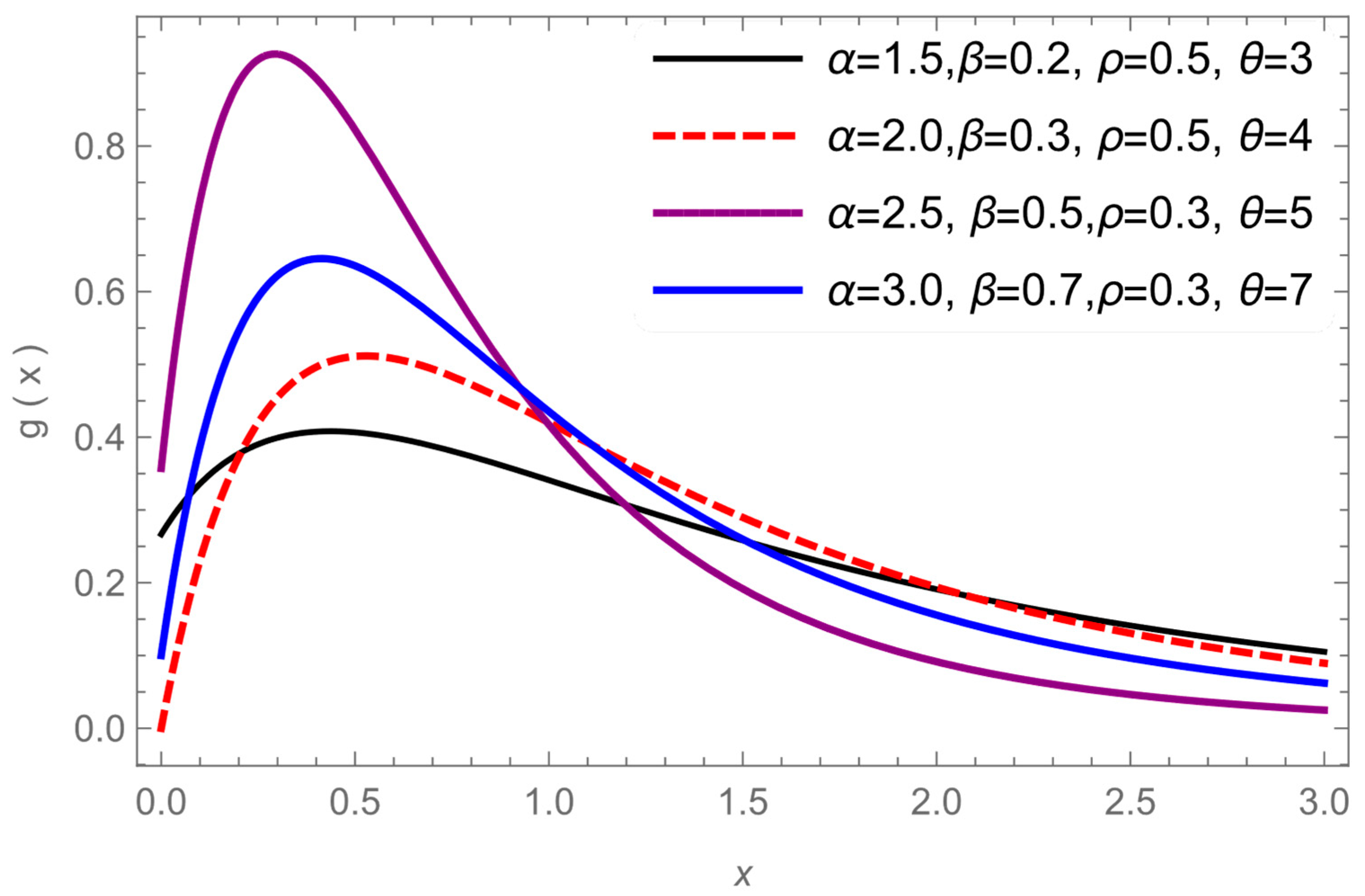
Also, when $\rho$ = 0, α = 0, the $\overline{G}\left(x,\alpha ,\beta ,\theta ,\rho \right)$ and $g\left(x\right)$, reduce to the Lomax distribution Lomax [26]. Figure 1 and Figure 2 give the graph MB-L PDF for values of, $\alpha , \beta , \theta$ and $\rho$.

Figure 1. Draw of decreasing MB-L PDF for values of $\alpha , \beta , \theta$ and $\rho$.

Figure 2. Draw of increasing-decreasing MB-L PDF for values of $\alpha , \beta , \theta$ and $\rho$.

Figure 1 and Figure 2 show different shapes of the PDF while it gives, a monotonic increasing, decreasing, constant and unimodal shapes, so we can conclude that the MB-L model is a very flexible distribution in modeling various type of data.

The next theorem gives the behavior of the MB-L PDF.

Theorem 1. 

For the MB-L ($\alpha ,\beta ,\theta ,\rho$) model, The PDF given by (4) is decreasing if $0<\theta <\frac{\alpha (1-\rho )(1+\alpha \rho )}{2+{\alpha }^2\left(\rho -1\right)\rho +\alpha (1+\rho )},$ independent of $\beta$ and is unimodal if $\theta >\frac{{\alpha }^2(\rho -1)}{2+{\alpha }^2\left(\rho -1\right)-\alpha (1+\rho )}$.

Proof. 

We can rewrite Equation (4) as:

$$g\left(x,\alpha ,\beta ,\theta ,\rho \right)=\frac{\alpha \beta \theta ({\left(1+x \beta \right)}^{2\theta }-\left(-1+\alpha +2{\left(1+x \beta \right)}^{\theta }\right)\rho +\alpha {\rho }^2)}{{\left(1+x \beta \right)}^{\theta +1}{(-1+\alpha +{\left(1+x \beta \right)}^{\theta }-\alpha \rho )}^2}$$

then,

$$\stackrel{`}{g}\left(x\right)=\frac{\alpha {\beta }^2\theta }{{(1+x\beta )}^2{(-1+\alpha (1-\rho )+{(1+x\beta )}^{\theta })}^3}\mathsf{\Phi }\left(x\right),\hspace{1em}x>0$$

where,

$$\begin{array}{l}\mathsf{\Phi }\left(x\right)=\alpha {\beta }^2\theta (2\theta ({(1+x\beta )}^{\theta }-\rho )(-1+\alpha +{(1+x\beta )}^{\theta }-\alpha \rho )-2\theta ({(1+x\beta )}^{2\theta }\\ \hspace{1em}\hspace{1em}\hspace{1em}\hspace{1em}\hspace{1em}-(-1+\alpha +2{(1+x\beta )}^{\theta })\rho +\alpha {\rho }^2)-{(1+x\beta )}^{-\theta }(1+\theta )(-1\\ \hspace{1em}\hspace{1em}\hspace{1em}\hspace{1em}\hspace{1em}+\alpha +{(1+x\beta )}^{\theta }-\alpha \rho )({(1+x\beta )}^{2\theta }-(-1+\alpha \\ \hspace{1em}\hspace{1em}\hspace{1em}\hspace{1em}\hspace{1em}+2{(1+x\beta )}^{\theta })\rho +\alpha {\rho }^2))\end{array}$$

if $\mathsf{\Phi }\left(0\right)=\alpha {\beta }^2\theta (\rho -1)(2\theta +{\alpha }^2\left(1+\theta \right)\left(1-\rho \right)\rho +\alpha (-1+\theta (1+\rho )+\rho \left)\right)\le 0$, then $\theta \ge \frac{\alpha (1-\rho )(1+\alpha \rho )}{2+{\alpha }^2\left(\rho -1\right)\rho +\alpha (1+\rho )}$, $\stackrel{`}{g}\left(x\right)<0$, then $g\left(x\right)$ is decreasing.

if $\mathsf{\Phi }\left(0\right)>0,$ then $\theta <\frac{\alpha (1-\rho )(1+\alpha \rho )}{2+{\alpha }^2\left(\rho -1\right)\rho +\alpha (1+\rho )},$ ${\displaystyle \underset{x\to \infty }{\lim }}g\left(x\right)=0,$ and ${\displaystyle \underset{x\to 0}{\lim }}g\left(x\right)=\frac{\beta \theta (1-(1+\alpha )\rho +\alpha {\rho }^2)}{\alpha {(1-\rho )}^2}$ then g(x), first increases than decrease to zero and hence has a mode $x_{mod}$ given by: $\mathsf{\Phi }\left(x_{mod}\right)=0$. Moreover, this mode is unique Dharmadhikari et al. [27]. □

Remark 1.

• For $\rho =0,\alpha =1,$ g(x) is decreasing (unimodal) if $\theta \le 1$ ($\theta >1$) which is the well-known result for the Lomax distribution.
• For $\rho =0,$ g(x) is decreasing if $\theta <\frac{-\alpha }{2-\alpha }$ (i.e., $\alpha +(2-\alpha )\theta \ge 0$) and is unimodal if $\theta >\frac{-\alpha }{2-\alpha }$ (i.e., $\alpha +(2-\alpha )\theta <0$) which is the well-known result for the MOEL distribution (Ghitany et al. [14]).

The ${\mathit{r}}^{\mathit{t}\mathit{h}}$ moment of MB-L model

For the MB-L ($\alpha ,\beta ,\theta ,\rho$) model, the $r^{th}$ moment $E\left(X^r\right),r\ge 1,$ is:

$$\begin{array}{l}E\left(X^r\right)=r{\displaystyle \underset{0}{\overset{\infty }{\int }}}{x}^{r-1}\overline{G}\left(x\right)dx\\ =r{\displaystyle \underset{0}{\overset{\infty }{\int }}}{x}^{r-1}\frac{\alpha {\left(1+\beta x\right)}^{-\theta }\left[1-\rho {\left(1+\beta x\right)}^{-\theta }\right]}{1-\left[1-\left(1-\rho \right)\alpha \right]{\left(1+\beta x\right)}^{-\theta }}dx\\ =\frac{r}{{\beta }^{r+2}\theta }{\displaystyle \sum _{u=0}^{\infty }}{\left(\left[1-\left(1-\rho \right)\alpha \right]\right)}^u{\displaystyle \underset{0}{\overset{1}{\int }}}{y}^{u-\frac{1}{\theta }}{\left(y^{-\frac{1}{\theta }}-1\right)}^r\left(1-\rho y\right)dy\\ =\frac{r}{{\beta }^{r+2}\theta }{\displaystyle \sum _{u=0}^{\infty }}{\left(\left[1-\left(1-\rho \right)\alpha \right]\right)}^u{(-1)}^r\theta \mathrm{Gamma}\left[1+r\right]\end{array}$$

The MGF of MB-L model

We present the MGF M (t, $\alpha ,\beta ,\theta ,\rho$) of the MB-L model. Using Equation (4), the substitution $u=(1+\beta x)$ and Maclaurin expansion of $e^x$ for all x, we get the following:

$$\begin{array}{ll}M\left(t,\alpha ,\beta ,\theta ,\rho \right)& =E\left(e^{tX}\right)\\ & ={\displaystyle \underset{0}{\overset{\infty }{\int }}}{e}^{tx}\frac{\alpha \beta \theta ({\left(1+x \beta \right)}^{2\theta }-\left(-1+\alpha +2{\left(1+x \beta \right)}^{\theta }\right)\rho +\alpha {\rho }^2)}{{\left(1+x\beta \right)}^{\theta +1}{(-1+\alpha +{\left(1+x \beta \right)}^{\theta }-\alpha \rho )}^2}dx\\ & ={\displaystyle \underset{1}{\overset{\infty }{\int }}}{e}^{\frac{t}{\beta }(u-1)}\frac{\alpha \theta ({\left(u\right)}^{2\theta }-\left(-1+\alpha +2{\left(u\right)}^{\theta }\right)\rho +\alpha {\rho }^2)}{{\left(u\right)}^{\theta +1}{(-1+\alpha +{\left(u\right)}^{\theta }-\alpha \rho )}^2}du\\ & =\alpha \theta e^{-\frac{t}{\beta }}{\displaystyle \underset{1}{\overset{\infty }{\int }}}{e}^{\frac{tu}{\beta }}\frac{\alpha \theta ({\left(u\right)}^{2\theta }-\left(-1+\alpha +2{\left(u\right)}^{\theta }\right)\rho +\alpha {\rho }^2)}{{\left(u\right)}^{\theta +1}{(-1+\alpha +{\left(u\right)}^{\theta }-\alpha \rho )}^2}\\ & =\alpha \theta e^{-\frac{t}{\beta }}{\displaystyle \sum _{i=0}^{\infty }}{\displaystyle \sum _{j=0}^{\infty }}\frac{{(\alpha \rho )}^j\left(\frac{t}{\beta }\right)\left(\frac{\alpha \rho }{\theta \left(j+2\right)-i}+\frac{1}{\theta \left(j+1\right)-i-1}\right)}{i!j!}.\end{array}$$

where $0<\alpha \rho <1.$ For more details of MGF see BS [28] and YF and SY [29].

Now we have the following results:

Theorem 2. 

For the SF (3) of MB-L model, if $X_i,i=1,2,\dots ,n$ are independent identically distributed (i.i.d), then ${\mathrm{U}}_{\mathrm{N}}=\min \left(X_1,X_2,\dots ,X_n\right),$ has the SF:

$${\overline{G}}_{{\mathrm{U}}_{\mathrm{N}}}\left(x,\alpha ,\beta ,\theta ,\rho \right)={\left(\frac{\alpha \left[1-\rho {(1+\beta x)}^{-\theta }\right]}{{(1+\beta x)}^{\theta }-\left[1-\left(1-\rho \right) \alpha \right]}\right)}^n.$$

Proof. 

We know that,

$$\overline{G}\left(x,\alpha ,\beta ,\theta ,\rho \right)=\frac{\alpha {(1+\beta x)}^{-\theta }\left[1-\rho {(1+\beta x)}^{-\theta }\right]}{1-\left[1-\left(1-\rho \right) \alpha \right] {(1+\beta x)}^{-\theta }}$$

$$\begin{array}{ll}{\overline{G}}_{{\mathrm{U}}_{\mathrm{N}}}\left(x,\alpha ,\beta ,\theta ,\rho \right)& =P\left(\min \left(X_1,X_2,\dots ,X_n\right)>x\right)\\ & ={\displaystyle \prod _{i=1}^n}\overline{G}\left(x,\alpha ,\beta ,\theta ,\rho \right)={\left(\frac{\alpha \left[1-\rho {(1+\beta x)}^{-\theta }\right]}{{(1+\beta x)}^{\theta }-\left[1-\left(1-\rho \right)\alpha \right]}\right)}^n.\square \end{array}$$

Theorem 3. 

For the SF (3) of MB-L model, if $X_i,i=1,2,\dots ,N$ are i.i.d, $N$ be a Markov Bernoulli geometric distribution with parameters $p,\rho$ such that:

$$P\left(N=n\right)=\left\{\begin{array}{ll}p,& n=1\\ \left(1-p\right)a^{-1}{\left(1-a^{-1}\right)}^{n-2},& n\ge 2,\end{array}\right.$$

which is independent of $X_i$ for all I = 1,2, …, N. Then, $U_N={\displaystyle \underset{1\le i\le N}{\min }}{X}_{i,}$ is distributed MB-L if $X_i$ is distributed as Lomax distribution.

Proof. 

Suppose that,

$$\begin{array}{ll}\overline{G}\left(x\right)=\mathit{Pr}\left(U_N>x\right)& =Pr\left(X_i>x_i,\hspace{1em}\hspace{1em}\hspace{1em}i=1,2,\dots ,N\right)={\displaystyle \sum _{n=1}^{\infty }}{\overline{F}}^n\left(x\right)\mathit{Pr}\left(N=n\right)\\ & =p\overline{F}\left(x\right)+\left(1-p\right)a^{-1}{\overline{F}}^2\left(x\right){\displaystyle \sum _{n=2}^{\infty }}{\overline{F}}^{n-2}\left(x\right){(1-a^{-1})}^{n-2}\\ & =p\overline{F}\left(x\right)+\left(1-p\right)a^{-1}{\overline{F}}^2\left(x\right)\frac{1}{[1-(1-a^{-1}\left)\overline{F}\left(x\right)\right]}\\ & =\frac{\overline{F}\left(x\right)[p-p\overline{F}\left(x\right)+a^{-1}\overline{F}\left(x\right)]}{[1-(1-a^{-1}\left)\overline{F}\left(x\right)\right]}, \mathrm{w}\mathrm{h}\mathrm{e}\mathrm{r}\mathrm{e} a^{-1}=\left(1-\rho \right)p\end{array}$$

hence,

$$\overline{G}\left(x\right)=\frac{p[1-\rho {\left(1+x\beta \right)}^{-\theta }]}{{\left(1+x\beta \right)}^{\theta }-(1-a^{-1})}$$

Which is MB-L mdel with $p=\alpha$. □

3. The HRF of the MB-L Model

From Equation (3) we have:

$$h\left(x\right)=\frac{\beta \theta ({(1+x\beta )}^{2\theta }-(-1+\alpha +2{(1+x\beta )}^{\theta })\rho +\alpha {\rho }^2)}{(1+x\beta )({(1+x\beta )}^{\theta }-\rho )(-1+\alpha +{(1+x\beta )}^{\theta }-\alpha \rho )}.$$

(5)

For all $\mathsf{\theta },\alpha >0,0<\rho <1,$ then,

$${\displaystyle \underset{x\to 0}{\lim }}h\left(x\right)=\frac{\beta \theta (-1+\alpha \rho )}{\alpha (-1+\rho )}, {\displaystyle \underset{x\to \infty }{\lim }}h\left(x\right)=0.$$

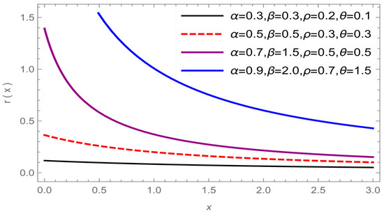
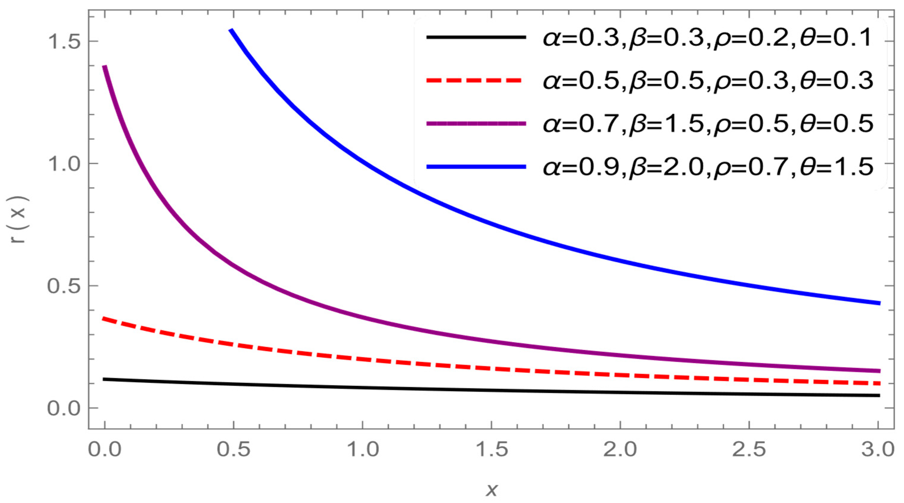
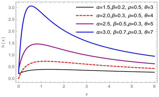
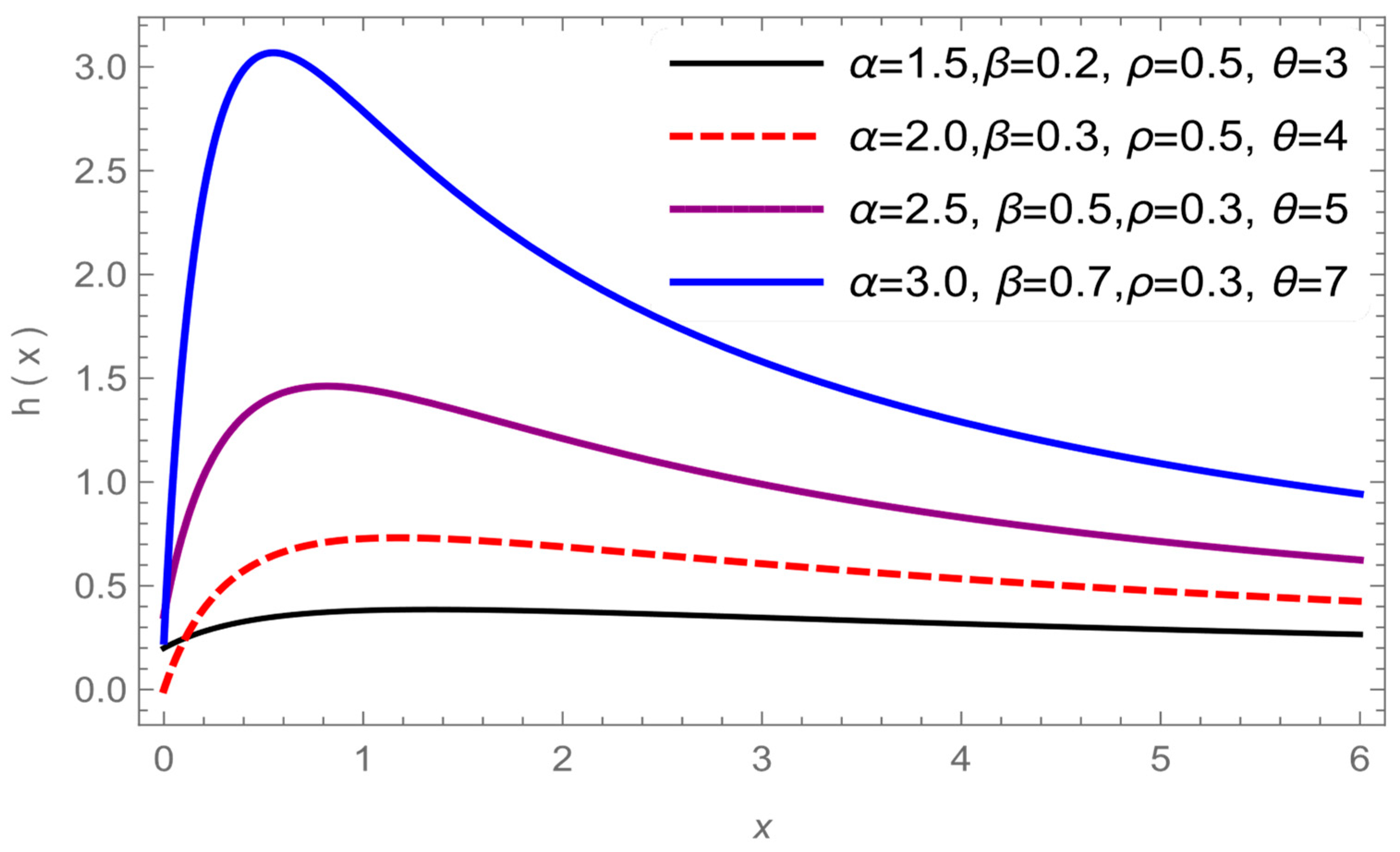
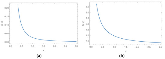
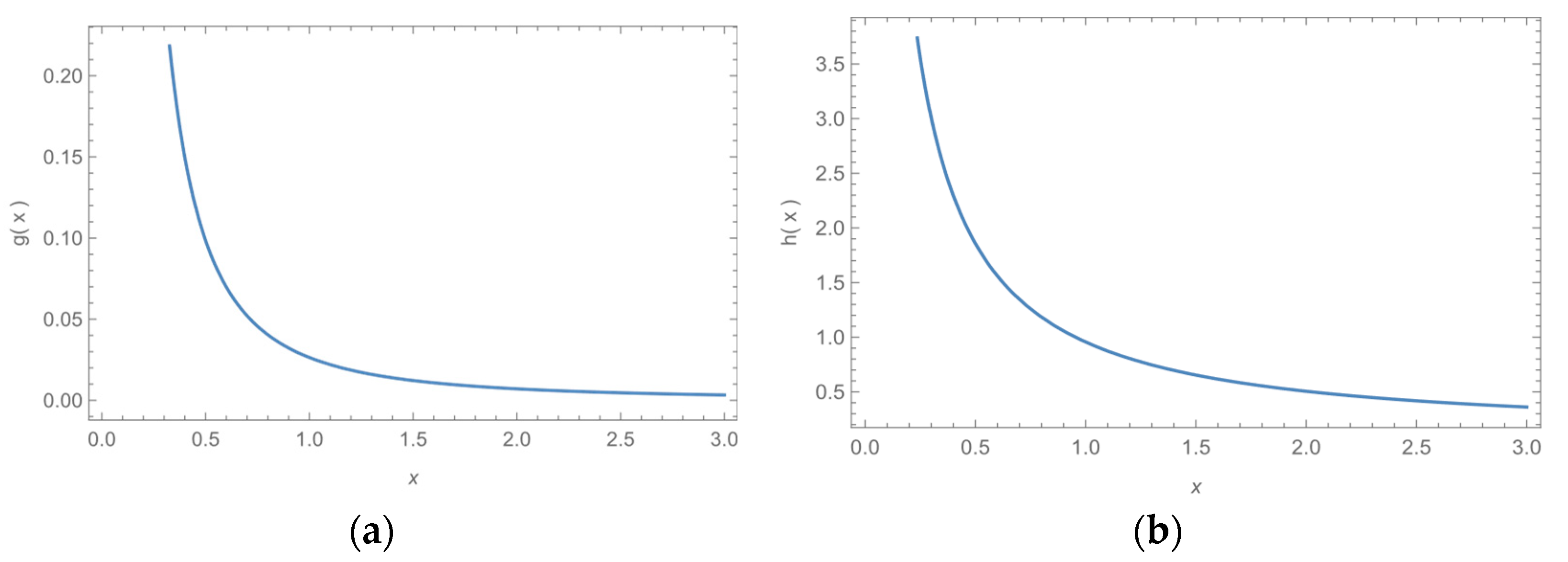
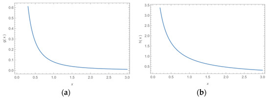
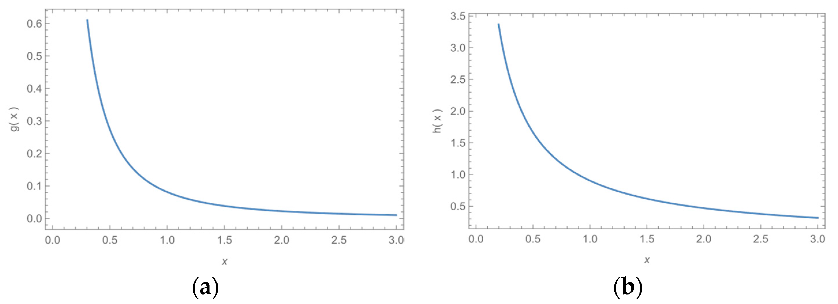
Figure 3 and Figure 4 show different shapes of the HRF while it gives, a monotonic increasing, decreasing, constant and unimodal shapes, so we can conclude that the HRF is a very flexible distribution in modeling various type of data.

Figure 3. Draw of decreasing HRF for values of $\alpha , \beta , \theta$ and $\rho$.

Figure 4. Draw of increasing-decreasing MB-L HRF for values of $\alpha , \beta , \theta$ and $\rho$.

Now we will study the behavior of HRF according to the following theorem:

Theorem 4.

For the MB-L ($\alpha ,\beta ,\theta ,\rho$) model, The HRF (3) is decreasing (unimodal) if $\theta \ge \frac{\alpha \left(1-\rho \right)\left(\alpha \rho -1\right)}{\left(1-{\alpha }^2\rho -\alpha \left(1-\rho \right)\right)}\left(\theta <\frac{\alpha \left(1-\rho \right)(\alpha \rho -1)}{(1-{\alpha }^2\rho -\alpha (1-\rho \left)\right)}\right)$ independent of $\beta$.

Proof. 

From Equation (3) we have:

$$\stackrel{`}{h}\left(x\right)=-\frac{{\beta }^2 \theta {(1+x\beta )}^{\theta }}{({\left(1+x\beta \right)}^2{\left({\left(1+x\beta \right)}^{\theta }-\rho \right)}^2{\left(-1+\alpha +{\left(1+x\beta \right)}^{\theta }-\alpha \rho \right)}^2))}\mathsf{\psi }(x)$$

(6)

where, $\mathsf{\psi }(x)=-\theta ({(1+x\beta )}^{2\theta }-\rho )(-1+\rho )-{\alpha }^2(1+\theta -\rho {(1+x\beta )}^{-\theta }){(-1+\rho )}^2\rho +$ $(-{(1+x\beta )}^{-\theta }+1)({(1+x\beta )}^{3\theta }+({(1+x\beta )}^{\theta }-3{(1+x\beta )}^{2\theta })\rho +(-1+2{(1+x\beta )}^{\theta }){\rho }^2)+$ $\alpha 1(-1+\rho )(-{(1+x\beta )}^{2\theta }+2(-1+2{(1+x\beta )}^{\theta })\rho +(2{(1+x\beta )}^{-\theta }-3){\rho }^2+\theta ({(1+x\beta )}^{2\theta }$ $-2\rho +{\rho }^2))]$

The proof is as in the Theorem 1. □

Remark 2.

• For $\rho =0,\alpha =1,$ $\theta \ge 1$ ($\theta <1$) h(x) is decreasing (unimodal). It is the same result for the Lomax distribution.
• For $\rho =0,$ h(x) is decreasing if $\theta \ge \frac{-\alpha }{1-\alpha }$ (i.e., $\alpha +(1-\alpha )\theta \ge 0$) and is unimodal if $\theta <\frac{-\alpha }{1-\alpha }$ (i.e., $\alpha +(1-\alpha )\theta <0$) which is the well-known result for the MOEL distribution.

4. Estimation of MB-L Parameters and Asymptotic Confidence Intervals (CI)

Here, the MLE for the MB-L Parameters are developed. Asymptotic confidence intervals of $\widehat{\mathsf{\psi }}=(\widehat{\alpha },\widehat{\beta },\widehat{\theta },\widehat{\rho })$ are obtained using the inverse Fisher’s information matrix elements. Simulation studies are carried out to investigate the accuracy of the estimates of the model’s parameter.

Suppose that ($t_1$, ${\delta }_1$), ($t_2$, ${\delta }_2$), …, ($t_n$, ${\delta }_n$) be a random sample from the MB-L ($\alpha ,\beta ,\theta ,\rho$) model, where ${\delta }_i=0$ or ${\delta }_i=1$ if $t_i$ are censored or complete observations, respectively.

The log-likelihood function for the MB-L ($\alpha ,\beta ,\theta ,\rho$) model is:

$$\begin{array}{cc}ln\left(t_i,\alpha ,\beta ,\theta ,\rho \right)=\hfill & {\displaystyle \sum _{i=1}^n}{\displaystyle \{}{\delta }_i\log \left[\frac{\alpha \beta \theta ({\left(1+x \beta \right)}^{2\theta }-\left(-1+\alpha (1+{\rho }^2)+2{\left(1+x \beta \right)}^{\theta }\right)\rho )}{{\left(1+x\beta \right)}^{\theta +1}{(-1+\alpha (1-\rho )+{\left(1+x \beta \right)}^{\theta })}^2}\right]\hfill \\ \hfill & +\left(1-{\delta }_i\right)\log \left[\frac{\alpha {(1+\beta x)}^{-\theta }\left[1-\rho {(1+\beta x)}^{-\theta }\right]}{1-\left[1-\left(1-\rho \right)\alpha \right]{(1+\beta x)}^{-\theta }}\right]{\displaystyle \}}\hfill \end{array}$$

The first derivative of $ln\left(t_i,\alpha ,\beta ,\theta ,\rho \right)$ with respect to $\alpha , \beta , \theta$ and $\rho$, respectively, are given by

$$\frac{\partial ln}{\partial \alpha }=0,\hspace{1em}\frac{\partial ln}{\partial \beta }=0,\hspace{1em}\frac{\partial ln}{\partial \theta }=0,\hspace{1em}\frac{\partial ln}{\partial \rho }=0.$$

The MLE $\widehat{\mathsf{\psi }}=(\widehat{\alpha },\widehat{\beta },\widehat{\theta },\widehat{\rho })$ can be obtained numerically using these equations. For the asymptotic CI, the normal approximation of the MLE can be used to construct asymptotic CIs for the parameters $\mathsf{\psi }$ when the sample size is large enough. A two-sided (1−α) 100% CIs for $\mathsf{\psi }$ are $(\widehat{\mathsf{\psi }}\pm Z_{\alpha /2}\sqrt{Var(\widehat{\mathsf{\psi }})})$, where $Var(\widehat{\mathsf{\psi }})$ are the asymptotic variances of $\widehat{\mathsf{\psi }}$.

To compare the MB-L model with MOEL and Lomax distributions, we used the likelihood ratio test (LRT) as:

First: the null hypothesis $H_{10}:\alpha =1,\rho =0$ (Lomax distribution). Under $H_{10}$ the likelihood ratio statistic: $A_1=-2\left[\ln (1,\widehat{\beta },\widehat{\theta },0)-\ln (\widehat{\alpha },\widehat{\beta },\widehat{\theta },\widehat{\rho })\right]$, it has a ${\chi }^2$ distribution with 2 degrees of freedom

Second: the null hypothesis $H_{20}:\rho =0$ (MOEL distribution). Under $H_{20}$ the likelihood ratio statistic: $A_2=-2\left[\ln (\widehat{\alpha },\widehat{\beta },\widehat{\theta },0)-\ln (\widehat{\alpha },\widehat{\beta },\widehat{\theta },\widehat{\rho })\right]$, which has an asymptotic ${\chi }^2$ distribution with 1 degree of freedom.

Also, the model selection: Akiake information criterion (AIC) (Akiake [30]), Bayesian information criterion (BIC) and Consistent Akaike Information Criteria $\left(\mathrm{C}\mathrm{A}\mathrm{I}\mathrm{C}\right)$ defined as:

$$AIC=\log likelihood-2k,$$

$$BIC=loglikelihood-\frac{k}{2}\log \left(n\right),$$

$$CAIC = 2 log likelihood-\frac{2kn}{n-k-1}.$$

where, k is the number of model parameters and n is the sample size. The model with higher AIC, CAIC and BIC is the one that better fits the data.

5. Simulation

The calculation of the estimation is based on N = 10,000 simulated samples from the MB-L model. The sample sizes are 50, 100, 200 and 300 and the parameter values are $\mathsf{\psi }=\left(\alpha ,\beta ,\theta ,\rho \right)=(0.7,1.2,0.05,0.03)$ and $(0.3,0.3,0.1,0.2)$. The validity of the estimate of $\mathsf{\psi }$ is studied by the following measures:

• Bias of $\mathsf{\psi }(\alpha ,\beta ,\theta ,\rho )$ is $\frac{1}{N}{\displaystyle {\sum }_{i=1}^N}(\widehat{\mathsf{\psi }}-\mathsf{\psi })$
• Mean square error (MSE) of $\mathsf{\psi }(\alpha ,\beta ,\theta ,\rho )$ is $\frac{1}{N}{{\displaystyle {\sum }_{i=1}^N}(\widehat{\mathsf{\psi }}-\mathsf{\psi })}^2.$
• Coverage probability (CP) of the N simulated confidence intervals.

When the n is large, the values of $\widehat{\mathsf{\psi }}$ are close to the initial values of $\mathsf{\psi }$ see Table 1.

Table 1. The MLE, bias, MSE and CP values for the MB-L ($\alpha ,\beta ,\theta ,\rho$) model.

n	Parameter	Initial	MLE	Bias	MSE	CP	Initial	MLE	Bias	MSE	CP
50	α	0.7	0.7070	0.0070	0.0031	0.9891	0.3	0.3041	0.00411	0.0008	0.9782
	β	1.2	1.1934	−0.0066	0.0009	0.9535	0.3	0.2981	−0.0019	0.0002	0.9643
	θ	0.05	0.6390	0.5890	0.3483	0.9852	0.1	0.4327	0.3327	0.1114	0.9665
	ρ	0.03	0.0337	0.0039	0.0007	0.9552	0.2	0.2331	0.0331	0.0207	0.9663
100	α	0.7	0.7008	0.0008	0.0009	0.9885	0.3	0.3047	0.0047	0.0004	0.9757
	β	1.2	1.203	0.0031	0.0004	0.9535	0.3	0.2975	−0.0025	0.0001	0.9527
	θ	0.05	0.6415	0.5914	0.3506	0.9764	0.1	0.4347	0.3347	0.1124	0.9791
	ρ	0.03	0.0296	−0.0004	0.0003	0.9574	0.2	0.2268	0.0268	0.0097	0.9546
200	α	0.7	0.7045	0.0045	0.0009	0.9999	0.3	0.3008	0.0008	0.0001	0.9887
	β	1.2	1.1991	−0.0009	0.0002	0.9573	0.3	0.2997	−0.0003	0.00005	0.9592
	θ	0.05	0.6368	0.5868	0.3447	0.9863	0.1	0.4376	0.3376	0.1142	0.9854
	ρ	0.03	0.0322	0.0022	0.0003	0.9583	0.2	0.2052	0.0052	0.0038	0.9575
300	α	0.7	0.7048	0.0048	0.0006	0.9992	0.3	0.2997	−0.0003	0.0001	0.9985
	β	1.2	1.1976	−0.0024	0.0001	0.9592	0.3	0.3002	0.0002	0.00003	0.9587
	θ	0.05	0.6363	0.5863	0.3440	0.9845	0.1	0.4368	0.3368	0.11354	0.9863
	ρ	0.03	0.0326	0.0026	0.0002	0.9547	0.2	0.2029	0.0029	0.0030	0.9638

6. Applications

6.1. Censored Data

Lee and Wang [31] P. 231 obtained the data which represent the 137-bladder cancer patient. This data has completed at 0.08 to 79.05 months and censored at 0.87, 3.02, 4.33, 4.65, 4.70, 8.60, 10.86, 19.36, 24.80 months. Table 2 shows values of MLE, Log-likelihood, AIC, BIC and CAIC of MB-L model with other models.

Table 2. MLE, standrd error (S.E), log-likelihood, AIC, BIC for MB-L, MOEL and Lomax models from the 137- censored data.

Model	Parameter	MLE	S.E	Log-Likelihood	AIC	BIC	CAIC
MB-L	α	2.9782	0.433	$-417.228$	$-426.229$	$-428.069$	$-424.467$
	θ	3.0578	0.231
	ρ	0.2449	0.031
	β	0.0927	0.005
MOEL	α	2.959	0.087	−419.842	$-426.287$	$-428.127$	$-426.590$
	θ	4.115	0.012
	β	0.058	0.004
Lomax	θ	3.733	0.036	$-422.348$	$-430.347$	$-432.188$	$-430.651$
	β	0.0325	0.006

We note that, AIC, BIC and CAIC of MB-L model more than the corresponding of the MOEL and Lomax distributions which means that MB-L model is better to fit for the given data. Moreover, the approximate 95% two-sided CI of the parameters $\alpha ,\beta ,\theta$ and $\rho$ are given respectively as [$2.075,3.88$], [$1.275,4.838$], [$0.147,0.342$] and [$0.006$,$0.179$].

For the given censored data, under ${\mathrm{H}}_{10}$ thus ${\mathrm{X}}_{L1}=-2[-422.348+417.228]=10.24$, then ${\mathrm{X}}_{L1}>{\displaystyle {\mathsf{\chi }}_{2,0.05}^2}=5.991$. Also, under ${\mathrm{H}}_{20}$ thus ${\mathrm{X}6}_{L2}=-2[-419.842+417.228)]=5.228$, then ${\mathrm{X}}_{L2}>{\displaystyle {\mathsf{\chi }}_{1,0.05}^2}=3.84.$ So, the LRT rejects the null hypothesis that the Lomax and MOEL models is proper for the specific data.

Now, suppose that $t_i$ and ${\delta }_i,$ $i=1,2,\dots ,n$ are, respectively, the ordered survival times and corresponding censoring indicators. The product-limit estimator or Kaplan-Meier estimator (KME) (Kaplan-Meier [32]) of a SF is:

$${\overline{G}}_n\left(t\right)={\displaystyle \prod _{\begin{array}{c}t:t_i\le t\\ i=1,\dots ,n\end{array}}}\left\{1-\frac{{\delta }_i}{n-i+1}\right\},t>0.$$

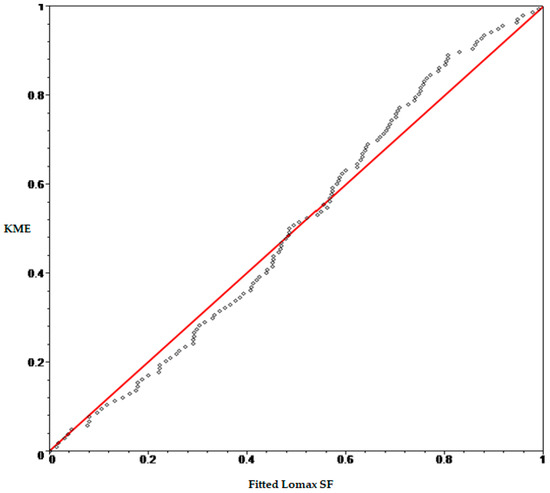
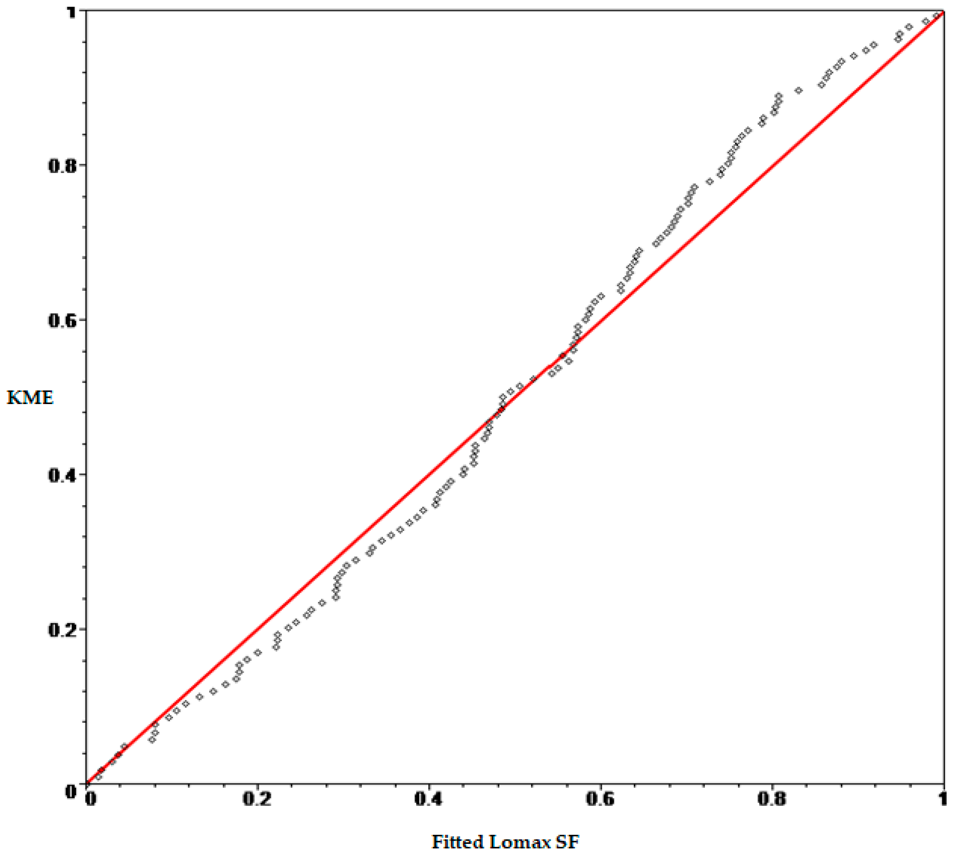
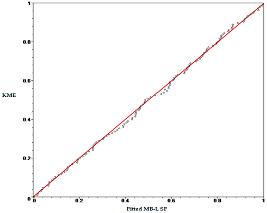
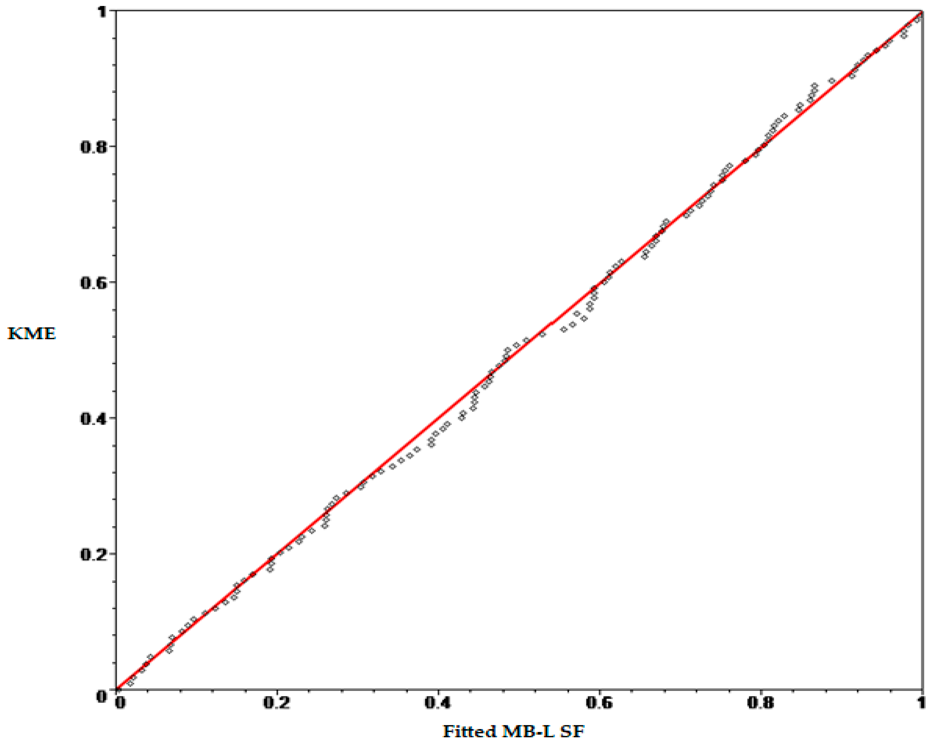
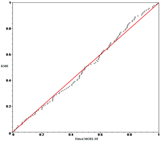
Figure 5, Figure 6 and Figure 7 show the probability-probability (P-P) plot of the KME versus the fitted Lomax, MOEL and MB-L SFs for 137 censored data.

Figure 5. P-P plot of KME and fitted Lomax SF.

Figure 6. P-P plot of KME and fitted MB-L SF.

Figure 7. P-P plot of KME and fitted MOEL SF.

From the previous figures, we notice that the drawn points for the fitted MB-L SF are close to the 45° line, indicating good fit as comparing with the fitted MB-L, MOEL and Lomax SFs.

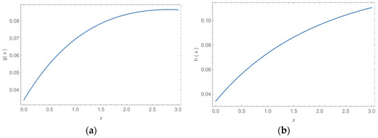
Since $\alpha =2.9782,\theta =3.0578,\rho =0.2449$ and $\beta =0.0927$, then the estimated hazard rate function ((a) MB-L model, (b) Lomax distribution) is as shown in the Figure 8.

Figure 8. The estimated hazard rate function of MB-L model from the given censored data.

6.2. COVID-19 Data

Applying the data from Huda M. Alshanbari et al. [33], which shows the two complete data of COVID-19 which represent a mortality rate.

First: COVID-19 data obtained through 37 days, from 27 June to 2 August 2021 (Saudi Arabia). The data and its measures show in Table 3 and Table 4.

Table 3. 37- COVID-19 data.

37 COVID-19 Data
0.0195	0.0213	0.0214	0.0217	0.0231	0.0233	0.0235	0.0235
0.0238	0.0239	0.0245	0.0260	0.0264	0.0268	0.0270	0.0271
0.0275	0.0278	0.0278	0.0282	0.0282	0.0285	0.0287	0.0294
0.0296	0.0300	0.0301	0.0309	0.0310	0.0313	0.0314	0.0315
0.0324	0.0325	0.0328	0.0332	0.0358

Table 4. MLE, S.E, log-likelihood, AIC, CAIC and BIC for MB-L, MOEL and Lomax models from COVID-19 data (Saudi Arabia).

Model	Parameter	MLE	S.E	Log-Likelihood	AIC	BIC	CAIC
MBEL	α	0.0103	0.033	$81.646$	$73.646$	$74.425$	$72.396$
	θ	4.1120	0.131
	ρ	0.4039	0.012
	β	0.0555	0.006
MOEL	α	0.1043	0.092	$79.529$	$73.529$	$74.113$	$72.802$
	θ	0.4901	0.211
	β	9.267	0.005
Lomax	θ	0.8213	0.321	$75.905$	$71.905$	$72.294$	$71.552$
	β	86.039	0.432

From this table, AIC, BIC and CAIC of MB-L model more than the corresponding of the MOEL and Lomax distributions which means that MB-L model is better to fit for the given data. Moreover, the approximate 95% two-sided CI of the parameters $\alpha ,\beta ,\theta$ and $\rho$ are given respectively as [$0.0049,0.0038$], [$0.068,0.563$], [$0.868,7.358$] and [$0.068,0.307$].

For the given 37 COVID-19 data, under ${\mathrm{H}}_{10}$ thus ${\mathrm{X}}_{L1}=-2[75.905-81.646]=11.482$, then ${\mathrm{X}}_{L1}>{\displaystyle {\mathsf{\chi }}_{2,0.05}^2}=5.991$. Also, under ${\mathrm{H}}_{20}$ thus ${\mathrm{X}}_{L2}=-2[79.529-81.646]=4.234$, then ${\mathrm{X}}_{L2}>{\displaystyle {\mathsf{\chi }}_{1,0.05}^2}=3.84$. So, the LRT rejects the null hypothesis that the Lomax and MOEL models is proper for the specific data. The estimated hazard rate function ((a) MB-L model, (b) Lomax distribution) is as shown in the Figure 9.

Figure 9. The estimated hazard rate function of MB-L model based on COVID-19 data (Saudi Arabia).

Second: COVID-19 data obtained during 172 days from the first of 1 March to 20 August 2020 (Italy). The data and its measures show in Table 5 and Table 6.

Table 5. 172- COVID-19 data.

172 COVID-19 Data
0.0107	0.0490	0.0601	0.0460	0.0533	0.0630	0.0297	0.0885
0.0540	0.1720	0.0847	0.0713	0.0989	0.0495	0.1025	0.1079
0.0984	0.1124	0.0807	0.1044	0.1212	0.1167	0.1255	0.1416
0.1315	0.1073	0.1629	0.1485	0.1453	0.2000	0.2070	0.1520
0.1628	0.1666	0.1417	0.1221	0.1767	0.1987	0.1408	0.1456
0.1443	0.1319	0.1053	0.1789	0.2032	0.2167	0.1387	0.1646
0.1375	0.1421	0.2012	0.1957	0.1297	0.1754	0.1390	0.1761
0.1119	0.1915	0.1827	0.1548	0.1522	0.1369	0.2495	0.1253
0.1597	0.2195	0.2555	0.1956	0.1831	0.1791	0.2057	0.2406
0.1227	0.2196	0.2641	0.3067	0.1749	0.2148	0.2195	0.1993
0.2421	0.2430	0.1994	0.1779	0.0942	0.3067	0.1965	0.2003
0.1180	0.1686	0.2668	0.2113	0.3371	0.1730	0.2212	0.4972
0.1641	0.2667	0.2690	0.2321	0.2792	0.3515	0.1398	0.3436
0.2254	0.1302	0.0864	0.1619	0.1311	0.1994	0.3176	0.1856
0.1071	0.1041	0.1593	0.0537	0.1149	0.1176	0.0457	0.1264
0.0476	0.1620	0.1154	0.1493	0.0673	0.0894	0.0365	0.0385
0.2190	0.0777	0.0561	0.0435	0.0372	0.0385	0.0769	0.1491
0.0802	0.0870	0.0476	0.0562	0.0138	0.0684	0.1172	0.0321
0.0327	0.0198	0.0182	0.0197	0.0298	0.0545	0.0208	0.0079
0.0237	0.0169	0.0336	0.0755	0.0263	0.0260	0.0150	0.0054
0.0375	0.0043	0.0154	0.0146	0.0210	0.0115	0.0052	0.2512
0.0084	0.0125	0.0125	0.0109	0.0071

Table 6. MLE, log-likelihood, AIC, CAIC and BIC for MB-L, MOEL and Lomax models from the COVID-19 data (Italy).

Model	Parameter	MLE	S.E	Log-Likelihood	AIC	BIC	CAIC
MB-L	α	0.3877	0.221	$154.215$	$146.215$	$143.920$	$145.976$
	θ	7.5606	0.431
	ρ	0.1028	0.023
	β	0.4824	0.321
MOEL	α	0.0013	0.006	$134.216$	$128.216$	$126.495$	$128.073$
	θ	1.0021	0.453
	β	0.0136	0.051
Lomax	θ	0.4751	0.254	$73.756$	$69.756$	$68.608$	$69.6845$
	β	71.702	0.534

From Table 6, AIC, BIC and CAIC of MB-L model more than the corresponding of the MOEL and Lomax models which means that MB-L Distribution is better to fit for the given data. In addition to, the approximate 95% two-sided CI of the parameters $\alpha ,\beta ,\theta$ and $\rho$ are given respectively as [$0.219,0.993$], [$0.188,0.776$], [$3.203,11.916$] and [$0.111,0.316$].

For the given 172 COVID-19 data, under ${\mathrm{H}}_{10}$ thus ${\mathrm{X}}_{L1}=-2\left[73.756-154.215\right]=160.918$, then ${\mathrm{X}}_{L1}>{\displaystyle {\mathsf{\chi }}_{2,0.05}^2}=5.991$. Also, under ${\mathrm{H}}_{20}$ thus ${\mathrm{X}}_{L2}=-2[134.216-154.215]=39.998$, then ${\mathrm{X}}_{L1}>{\displaystyle {\mathsf{\chi }}_{1,0.05}^2}=3.84$. So, the LRT rejects the null hypothesis that the Lomax and MOEL models is proper for the specific data. The estimated hazard rate function ((a) MB-L model, (b) Lomax distribution) is as shown in the Figure 10.

Figure 10. The estimated hazard rate function of MB-L model based on COVID-19 data (Italy).

7. Conclusions

In this paper, we introduced a four-parameter continuous distribution that generalizes MOEL and Lomax distributions. The new model is referred to as MB-L distribution, the derived properties including PDF, HRF, moments, MGF and minimum (maximum) MBG stable. The MLE procedure is straightforward. The active fitting of MB-L distribution is shown on bladder cancer and COVID-19 applications. We note that the value of the selected model choices is higher for MB-L distribution than for the MOEL and Lomax distributions. Furthermore, the relationship between the empirical and fitted SFs for MB-L distribution is higher compared to MOEL and Lomax distributions. All previous results indicate the advantage of MB-L distribution for bladder cancer and COVID-19 data.

References

- Gharib, M.; Mohammed, B.I.; Al-Ajmi, K.A.H. A New Method for Adding Two Parameters to a Family of Distributions with Application. J. Stat. Appl. Pro. 2017, 6, 487–497. [Google Scholar] [CrossRef] [Scilit]
- Marshall, A.W.; Olkin, I. A new method for adding a parameter to a family of distributions with application to the exponential and Weibull families. Biometrika 1997, 84, 641–652. [Google Scholar] [CrossRef] [Scilit]
- Johnson, N.L.; Kotz, S.; Balakrishnan, N. Contineous Univariate Distributions, 2nd ed.; Wiley: New York, NY, USA, 1994; Volume 1. [Google Scholar]
- Harris, C.M. The Pareto Distribution as a Queue Service Discipline. Oper. Res. 1968, 16, 307–313. [Google Scholar] [CrossRef] [Scilit]
- Bryson, M. Heavy tailed distributions: Properties and tests. Technometrics 1974, 16, 61–68. [Google Scholar] [CrossRef]
- Cordeiro, G.M.; Ortega, E.M.; Popović, B.V. The gamma-Lomax distribution. J. Stat. Comput. Simul. 2013, 85, 305–319. [Google Scholar] [CrossRef] [Scilit]
- Devi, B.; Kumar, P.; Kour, K. Entropy of Lomax Probability Distribution and its Order Statistic. Int. J. Stat. Syst. 2017, 12, 175–181. [Google Scholar]
- Maurya, R.K.; Tripathi, Y.M.; Lodhi, C.; Rastogi, M.K. On a generalized Lomax distribution. Int. J. Syst. Assur. Eng. Manag. 2019, 10, 1091–1104. [Google Scholar] [CrossRef] [Scilit]
- Mohammed, B.I.; Abu-Youssef, S.E.; Sief, M.G. A New Class with Decreasing Failure Rate Based on Countable Mixture and Its Application to Censored Data. J. Test. Eval. 2019, 48, 273–288. [Google Scholar] [CrossRef] [Scilit]
- Haq, M.A.U.; Rao, G.S.; Albassam, M.; Aslam, M. Marshall–Olkin Power Lomax distribution for modeling of wind speed data. Energy Rep. 2020, 6, 1118–1123. [Google Scholar] [CrossRef] [Scilit]
- Aryuyuen, S.; Bodhisuwan, W. The Type II Topp Leone-Power Lomax Distribution with Analysis in Lifetime Data. J. Stat. Theory Pract. 2020, 14, 31. [Google Scholar] [CrossRef] [Scilit]
- Alshanbari, H.M.; Ijaz, M.; Asim, S.M.; Hosni El-Bagoury, A.A.-A.; Dar, J.G. New Weighted Lomax (NWL) Distribution with Applications to Real and Simulated Data. Math. Probl. Eng. 2021, 2021, 8558118. [Google Scholar] [CrossRef] [Scilit]
- Dey, S.; Altun, E.; Kumar, D.; Ghosh, I. The Reflected-Shifted-Truncated Lomax Distribution: Associated Inference with Applications. Ann. Data Sci. 2021, 2021, 1. [Google Scholar] [CrossRef] [Scilit]
- Ghitany, M.E.; Al-Awadhi, F.A.; Alkhalfan, L.A. Marshall–Olkin Extended Lomax Distribution and Its Application to Censored Data. Commun. Stat. Theory Methods 2007, 36, 1855–1866. [Google Scholar] [CrossRef] [Scilit]
- Lemonte, A.J.; Cordeiro, G.M. An extended Lomax distribution. Statistics 2013, 47, 800–816. [Google Scholar] [CrossRef] [Scilit]
- Cordeiro, G.; Alizadeh, M.; Marinho, P. The type I half-logistic family of distributions. J. Stat. Comput. Simul. 2016, 86, 707–728. [Google Scholar] [CrossRef] [Scilit]
- Al-Zahrani, B.; Sagor, H. Statistical analysis of the Lomax–Logarithmic distribution. J. Stat. Comput. Simul. 2014, 85, 1883–1901. [Google Scholar] [CrossRef] [Scilit]
- Al-Zahrani, B.; Sagor, H. The Poisson-Lomax Distribution. Rev. Colomb. Estadística 2014, 37, 225–245. [Google Scholar] [CrossRef] [Scilit]
- Tahir, M.H.; Cordeiro, G.M.; Mansoor, M.; Zubair, M. Weibull-Lomax distribution: Properties and applications. Hacet. J. Math. Stat. 2015, 44, 455–474. [Google Scholar] [CrossRef] [Scilit]
- El-Bassiouny, A.; Abdo, N.F.; Shahen, H.S. Exponential lomax distribution. Int. J. Comput. Appl. 2015, 121, 24–29. [Google Scholar]
- Rady, E.-H.A.; Hassanein, W.A.; Elhaddad, T.A. The power Lomax distribution with an application to bladder cancer data. Springerplus 2016, 5, 1838. [Google Scholar] [CrossRef] [Scilit]
- Cooray, K. Analyzing lifetime data with long-tailed skewed distribution: The logistic-sinh family. Stat. Model. 2005, 5, 343–358. [Google Scholar] [CrossRef] [Scilit]
- Abu El Azm, W.S.; Almetwally, E.M.; Al-Aziz, S.N.; El-Bagoury, A.A.-A.H.; Alharbi, R.; Abo-Kasem, O.E. A New Transmuted Generalized Lomax Distribution: Properties and Applications to COVID-19 Data. Comput. Intell. Neurosci. 2021, 2021, 5918511. [Google Scholar] [CrossRef] [Scilit]
- Alsuhabi, H.; Alkhairy, I.; Almetwally, E.M.; Almongy, H.M.; Gemeay, A.M.; Hafez, E.; Aldallal, R.; Sabry, M. A superior extension for the Lomax distribution with application to Covid-19 infections real data. Alex. Eng. J. 2022, 61, 11077–11090. [Google Scholar] [CrossRef] [Scilit]
- Ogunde, A.A.; Chukwu, A.U.; Oseghale, I.O. The Kumaraswamy Generalized Inverse Lomax distribution and applications to reliability and survival data. Sci. Afr. 2023, 19. [Google Scholar] [CrossRef] [Scilit]
- Lomax, K.S. Business failures: Another example of the analysis of failure data. J. Am. Stat. Assoc. 1954, 45, 21–29. [Google Scholar] [CrossRef]
- Dharmadhikari, S.; Joag-dev, K. Unimodality, Convexity, and Applications; Academic Press: Cambridge, MA, USA, 1998. [Google Scholar]
- Simsek, B. Formulas Derived from Moment Generating Functions And Bernstein Polynomials, Applicable Analysis and Discrete Mathematics. Appl. Anal. Discret. Math. 2019, 13, 839–848. [Google Scholar] [CrossRef] [Scilit]
- Yalcin, F.; Simsek, Y. Formulas for characteristic function and moment generating functions of beta type distribution. Rev. Real Acad. Cienc. Exactas Físicas Y Naturales. Ser. A Matemáticas 2022, 116, 86. [Google Scholar] [CrossRef] [Scilit]
- Akaike, H. Fitting Autoregressive Models for Prediction. Ann. Inst. Stat. Math. 1969, 21, 243–247. [Google Scholar] [CrossRef] [Scilit]
- Lee, E.T.; Wang, J.W. Statistical Methods for Survival Data Analysis, 3rd ed.; John Wiley & Sons: Hoboken, NJ, USA, 2003; Volume 476. [Google Scholar]
- Kaplan, E.L.; Meier, P. Nonparametric Estimation from Incomplete Observations. J. Am. Stat. Assoc. 1958, 53, 457–481. [Google Scholar] [CrossRef]
- Alshanbari, H.M.; Odhah, O.H.; Almetwally, E.M.; Hussam, E.; Kilai, M.; El-Bagoury, A.-A.H. Novel Type I Half Logistic Burr-Weibull Distribution: Application to COVID-19 Data. Comput. Math. Methods Med. 2022, 2022, 1444859. [Google Scholar] [CrossRef] [Scilit]
Disclaimer/Publisher’s Note: The statements, opinions and data contained in all publications are solely those of the individual author(s) and contributor(s) and not of MDPI and/or the editor(s). MDPI and/or the editor(s) disclaim responsibility for any injury to people or property resulting from any ideas, methods, instructions or products referred to in the content. |
© 2023 by the authors. Licensee MDPI, Basel, Switzerland. This article is an open access article distributed under the terms and conditions of the Creative Commons Attribution (CC BY) license (https://creativecommons.org/licenses/by/4.0/).