Developing a Deep Learning-Based Defect Detection System for Ski Goggles Lenses
Abstract
1. Introduction
- Deep Learning Algorithms: Deep learning-based defect detection typically requires training object detection models or alternative specialized architectures on the extensively labeled datasets of defect images. Object detection methodologies have been extensively applied in the detection of defects on the surfaces of industrial products, such as steel, plastic, wood, and silk [10,11,12]. The task of object detection in computer vision encompasses two primary functions: localization [13] and classification [14]. In traditional computer vision, classifiers [15] such as SVM, KNN, and K-means clustering have played a vital role in categorizing classes. Meanwhile, object localization mainly employs fast template-matching-based algorithms [16].
- (1)
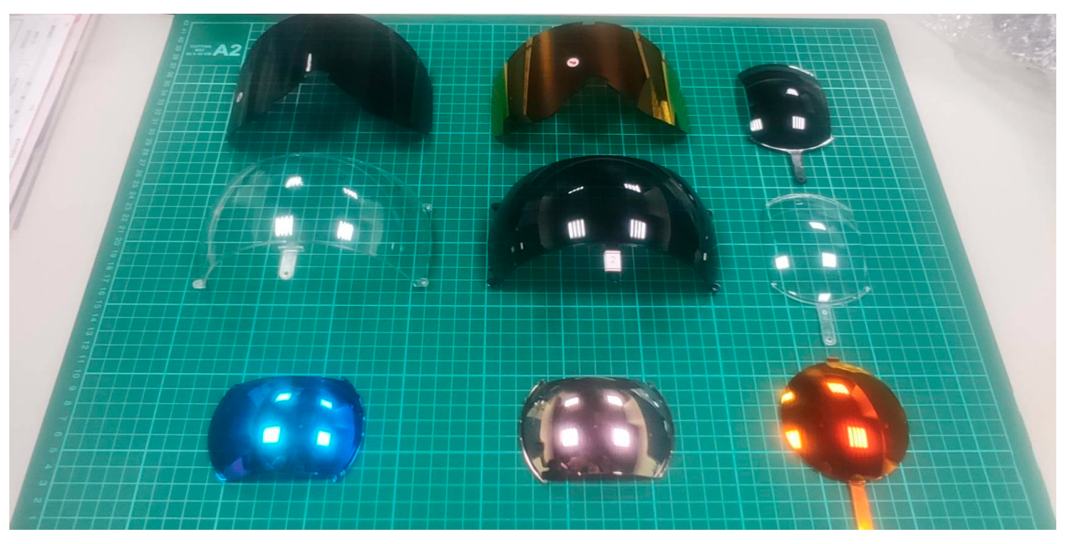
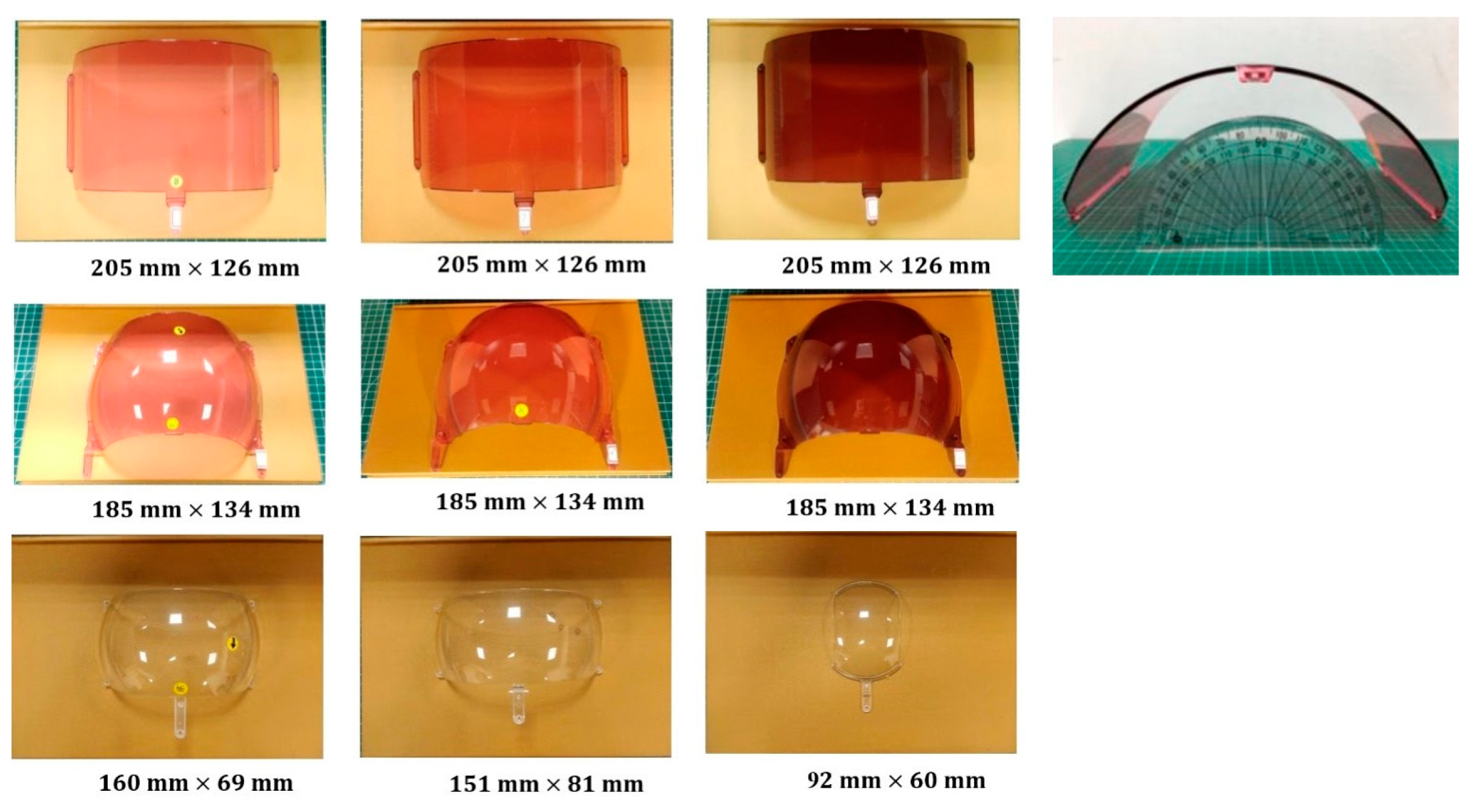
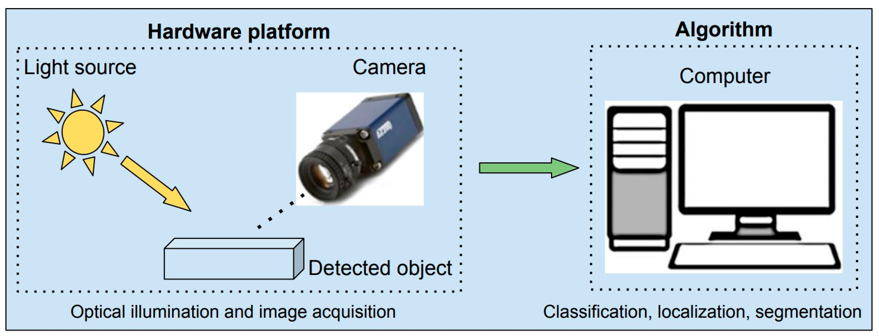
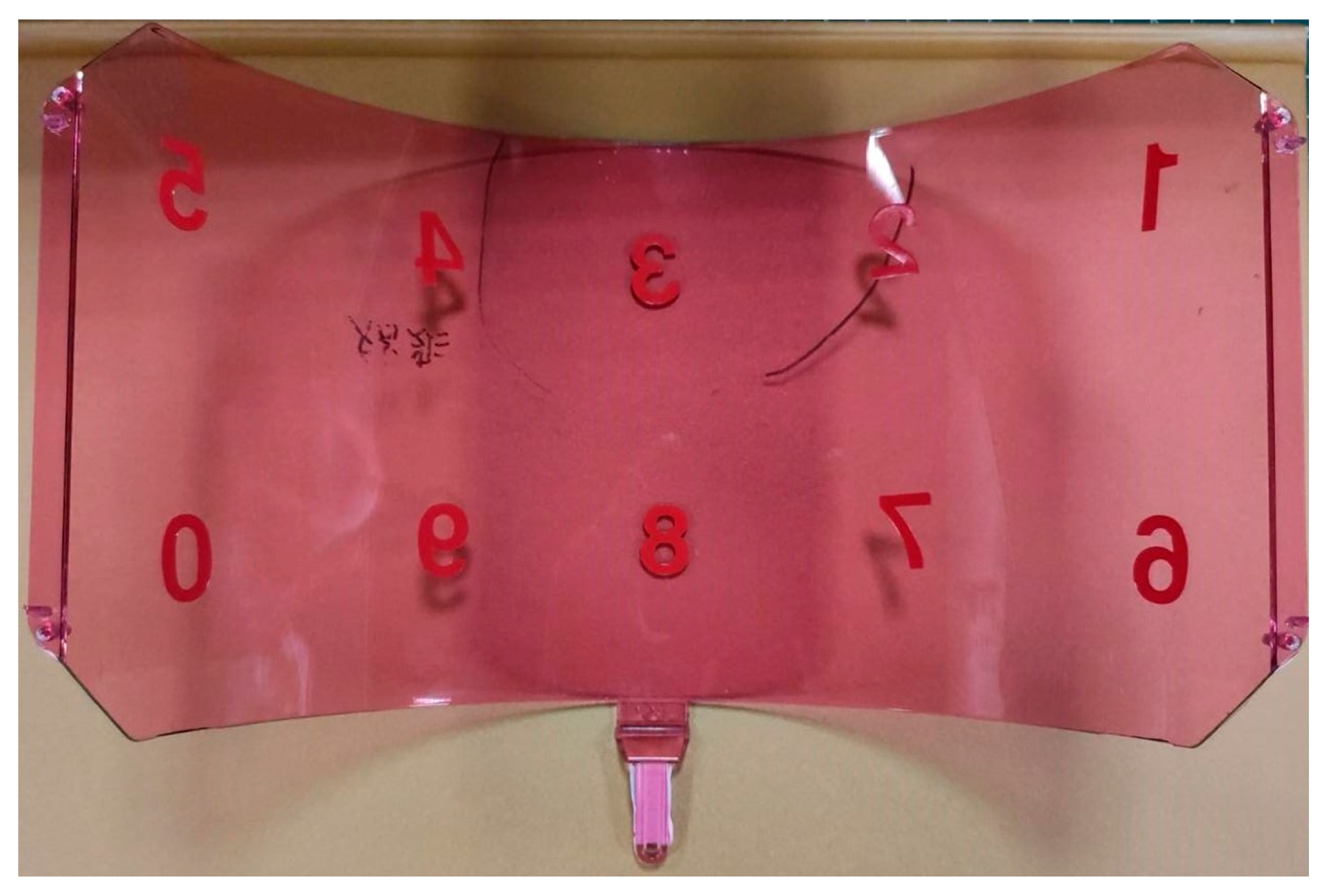
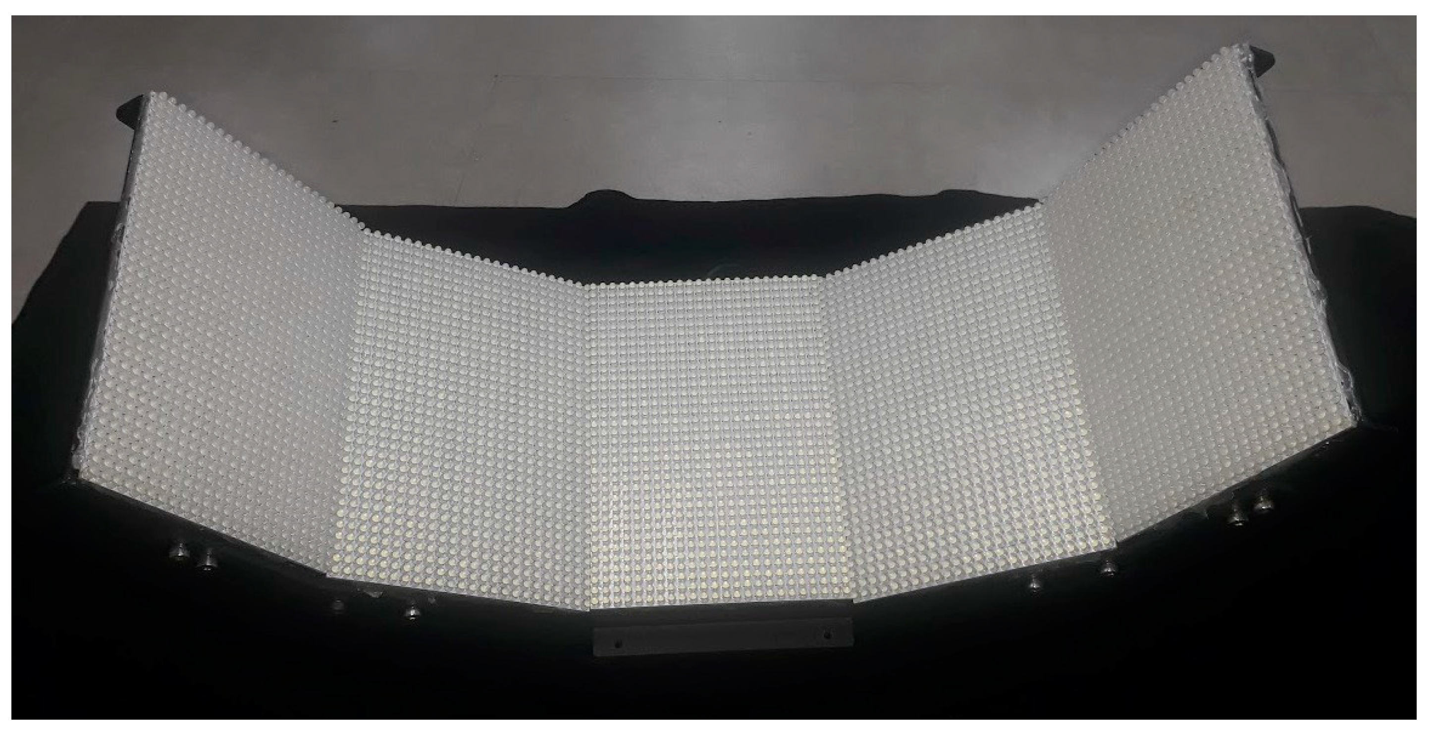
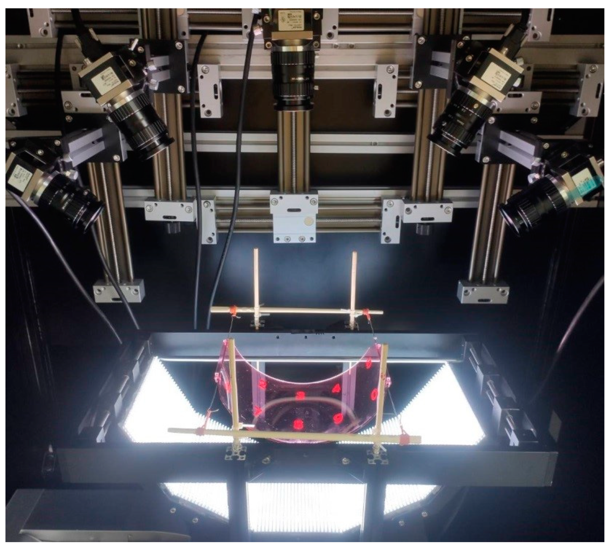
- Design of an image acquisition model that integrates cameras and light sources to effectively capture the entire surface of ski goggles lenses.
- (2)
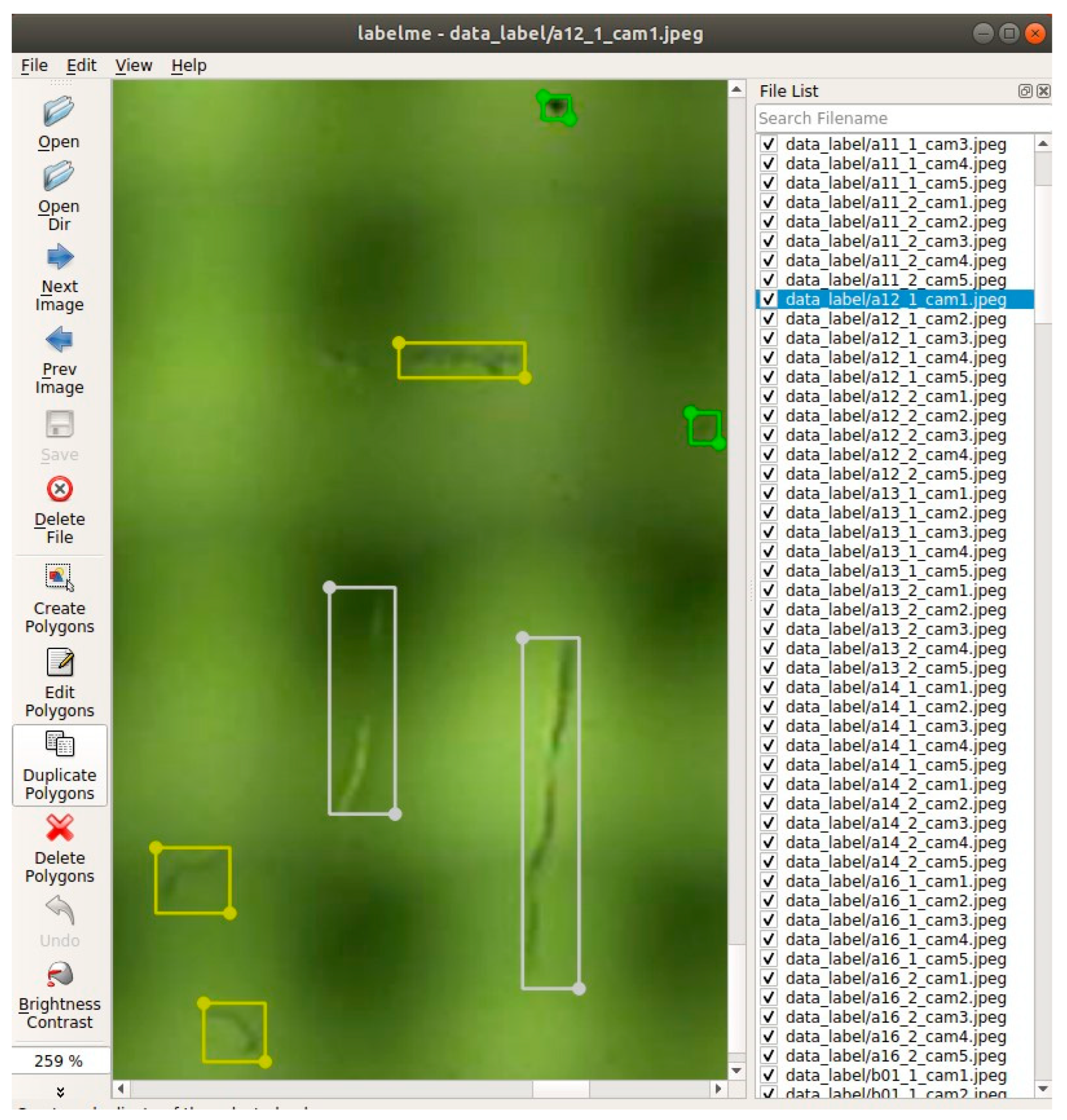
- Identification of lens defect categories and construction of a comprehensive ski goggles lens defect dataset.
- (3)
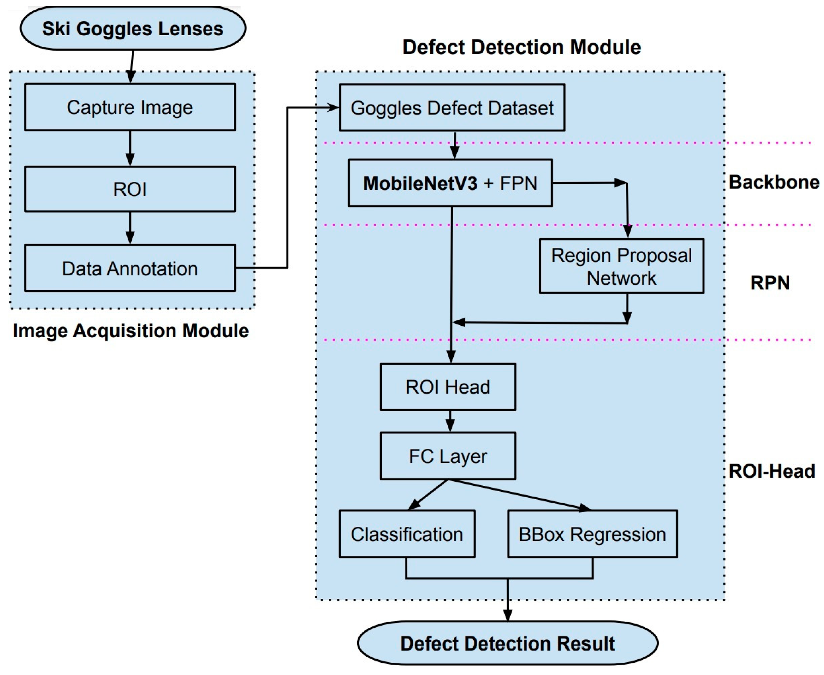
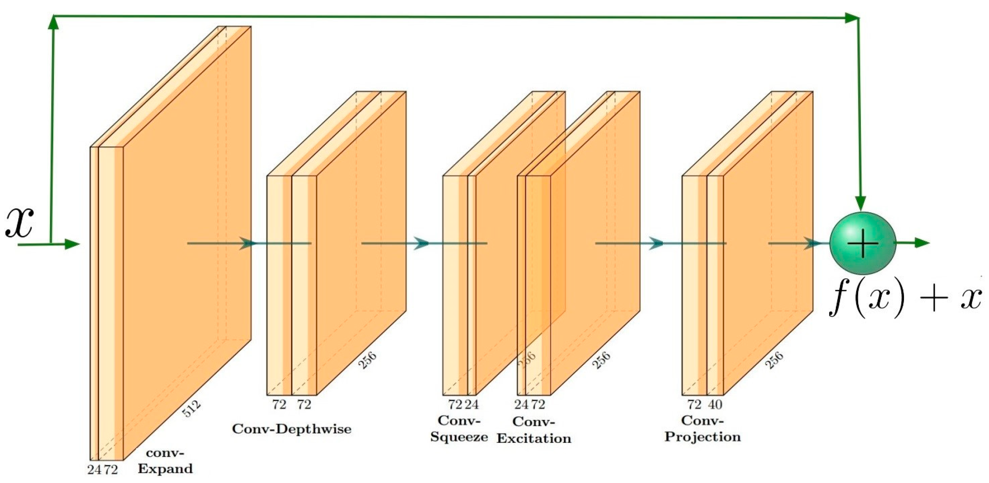
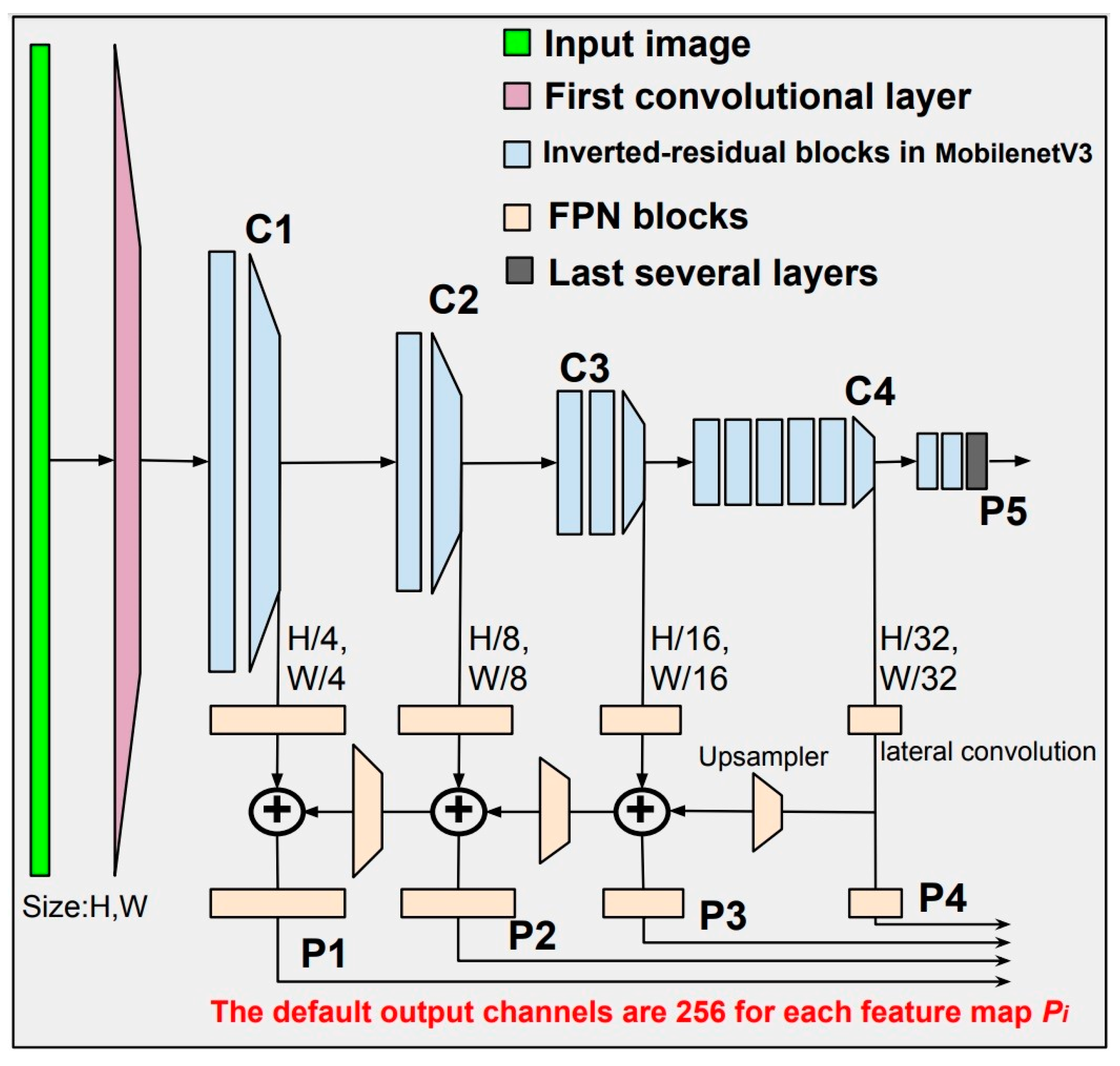
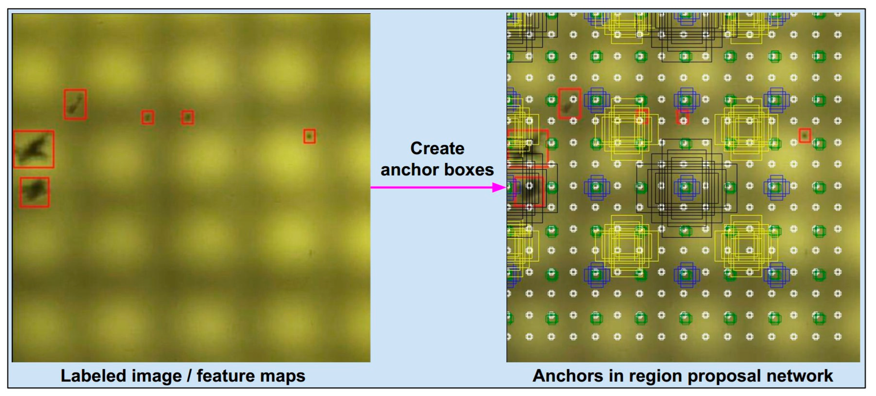
- Fine-tuning of the integrated object detection model that combines Faster R-CNN, FPN, and MobileNetV3 by implementing the following modifications: replacement of the default ResNet50 backbone with a combination of MobileNetV3 and feature pyramid network (FPN) to optimize computational efficiency and performance; adjustment of the region proposal network (RPN) hyperparameters to accommodate the detection of minuscule defects; and a reduction of the output channel count in the FPN to enhance computational performance without sacrificing accuracy.
2. Materials and Methods
2.1. Image Acquisition Module
2.1.1. Capture Image
2.1.2. Regions of Interest
2.1.3. Data Labeling
2.2. Defect Detection Module
2.2.1. Object Detection Problem Setting Based on Supervised Learning Approach
2.2.2. Backbone: Feature Extractor Based on MobileNetV3 and Feature Pyramid Networks
2.2.3. RPN: Region Proposal Network
2.2.4. Bounding Box Regression
2.2.5. ROI-Head
2.2.6. End-to-End Learning
3. Results
3.1. Experimental Setting
3.2. Defect Detection Results
4. Discussion
5. Conclusions
Author Contributions
Funding
Data Availability Statement
Acknowledgments
Conflicts of Interest
References
- Dang, D.-T.; Wang, J.-W.; Lee, J.-S.; Wang, C.-C. Defect Classification System for Ski Goggle Lens. In Proceedings of the 2021 International Symposium on Intelligent Signal Processing and Communication Systems (ISPACS), Hualien, Taiwan, 16–19 November 2021; pp. 1–3. [Google Scholar]
- Le, N.T.; Wang, J.-W.; Wang, C.-C.; Nguyen, T.N. Novel Framework Based on HOSVD for Ski Goggles Defect Detection and Classification. Sensors 2019, 19, 5538. [Google Scholar] [CrossRef] [PubMed]
- Luo, Q.; Fang, X.; Su, J.; Zhou, J.; Zhou, B.; Yang, C.; Liu, L.; Gui, W.; Tian, L. Automated Visual Defect Classification for Flat Steel Surface: A Survey. IEEE Trans. Instrum. Meas. 2020, 69, 9329–9349. [Google Scholar] [CrossRef]
- Luo, Q.; Fang, X.; Liu, L.; Yang, C.; Sun, Y. Automated Visual Defect Detection for Flat Steel Surface: A Survey. IEEE Trans. Instrum. Meas. 2020, 69, 626–644. [Google Scholar] [CrossRef]
- Peres, R.S.; Jia, X.; Lee, J.; Sun, K.; Colombo, A.W.; Barata, J. Industrial Artificial Intelligence in Industry 4.0—Systematic Review, Challenges and Outlook. IEEE Access 2020, 8, 220121–220139. [Google Scholar] [CrossRef]
- Hirschberg, I.; Bashe, R. Charge Coupled Device (CCD) Imaging Applications—A Modular Approach. In Applications of Electronic Imaging Systems; Franseen, R.E., Schroder, D.K., Eds.; SPIE: Bellingham, WA, USA, 1978; Volume 0143, pp. 11–18. [Google Scholar]
- Martins, R.; Nathan, A.; Barros, R.; Pereira, L.; Barquinha, P.; Correia, N.; Costa, R.; Ahnood, A.; Ferreira, I.; Fortunato, E. Complementary Metal Oxide Semiconductor Technology with and on Paper. Adv. Mater. 2011, 23, 4491–4496. [Google Scholar] [CrossRef] [PubMed]
- Mersch, S. Overview of Machine Vision Lighting Techniques. In Optics, Illumination, and Image Sensing for Machine Vision; Svetkoff, D.J., Ed.; SPIE: Bellingham, WA, USA, 1987; Volume 0728, pp. 36–38. [Google Scholar]
- Sieczka, E.J.; Harding, K.G. Light source design for machine vision. In Optics, Illumination, and Image Sensing for Machine Vision VI; Svetkoff, D.J., Ed.; SPIE: Bellingham, WA, USA, 1992; Volume 1614, pp. 2–10. [Google Scholar]
- He, Z.; Liu, Q. Deep Regression Neural Network for Industrial Surface Defect Detection. IEEE Access 2020, 8, 35583–35591. [Google Scholar] [CrossRef]
- Li, G.; Shao, R.; Wan, H.; Zhou, M.; Li, M. A Model for Surface Defect Detection of Industrial Products Based on Attention Augmentation. Comput. Intell. Neurosci. 2022, 2022, 9577096. [Google Scholar] [CrossRef] [PubMed]
- Zhang, D.; Hao, X.; Liang, L.; Liu, W.; Qin, C. A novel deep convolutional neural network algorithm for surface defect detection. J. Comput. Des. Eng. 2022, 9, 1616–1632. [Google Scholar] [CrossRef]
- He, Y.; Zhu, C.; Wang, J.; Savvides, M.; Zhang, X. Bounding Box Regression with Uncertainty for Accurate Object Detection. In Proceedings of the 2019 IEEE/CVF Conference on Computer Vision and Pattern Recognition (CVPR), Long Beach, CA, USA, 15–19 June 2019; pp. 2883–2892. [Google Scholar]
- Touvron, H.; Vedaldi, A.; Douze, M.; Jegou, H. Fixing the train-test resolution discrepancy. In Advances in Neural Information Processing Systems; Wallach, H., Larochelle, H., Beygelzimer, A., d’Alché-Buc, F., Fox, E., Garnett, R., Eds.; Curran Associates, Inc.: Red Hook, NY, USA, 2019; Volume 32, Available online: https://proceedings.neurips.cc/paper/2019/file/d03a857a23b5285736c4d55e0bb067c8-Paper.pdf (accessed on 5 November 2022).
- Okwuashi, O.; Ndehedehe, C.E. Deep support vector machine for hyperspectral image classification. Pattern Recognit. 2020, 103, 107298. [Google Scholar] [CrossRef]
- Jiao, J.; Wang, X.; Deng, Z.; Cao, J.; Tang, W. A fast template matching algorithm based on principal orientation difference. Int. J. Adv. Robot. Syst. 2018, 15, 1729881418778223. [Google Scholar] [CrossRef]
- He, K.; Zhang, X.; Ren, S.; Sun, J. Deep Residual Learning for Image Recognition. In Proceedings of the 2016 IEEE Conference on Computer Vision and Pattern Recognition (CVPR), Las Vegas, NV, USA, 27–30 June 2016; pp. 770–778. [Google Scholar]
- Simonyan, K.; Zisserman, A. Very Deep Convolutional Networks for Large-Scale Image Recognition. In Proceedings of the 3rd International Conference on Learning Representations (ICLR 2015), San Diego, CA, USA, 7–9 May 2015; Conference Track Proceedings. Bengio, Y., LeCun, Y., Eds.; 2015. [Google Scholar]
- Tan, M.; Le, Q. EfficientNet: Rethinking Model Scaling for Convolutional Neural Networks. In Proceedings of Machine Learning Research, Proceedings of the 36th International Conference on Machine Learning, Long Beach, CA, USA, 10–15 June 2019; Chaudhuri, K., Salakhutdinov, R., Eds.; PMLR: London, UK, 2019; Volume 97, pp. 6105–6114. [Google Scholar]
- Dosovitskiy, A.; Beyer, L.; Kolesnikov, A.; Weissenborn, D.; Zhai, X.; Unterthiner, T.; Dehghani, M.; Minderer, M.; Heigold, G.; Gelly, S.; et al. An Image is Worth 16 × 16 Words: Transformers for Image Recognition at Scale. arXiv 2021, arXiv:2010.11929. [Google Scholar]
- Zhang, S.; Chi, C.; Yao, Y.; Lei, Z.; Li, S.Z. Bridging the Gap Between Anchor-Based and Anchor-Free Detection via Adaptive Training Sample Selection. In Proceedings of the 2020 IEEE/CVF Conference on Computer Vision and Pattern Recognition (CVPR), Seattle, WA, USA, 13–19 June 2020; pp. 9756–9765. [Google Scholar]
- Ren, S.; He, K.; Girshick, R.; Sun, J. Faster R-CNN: Towards Real-Time Object Detection with Region Proposal Networks. IEEE Trans. Pattern Anal. Mach. Intell. 2017, 39, 1137–1149. [Google Scholar] [CrossRef]
- Redmon, J.; Divvala, S.; Girshick, R.; Farhadi, A. You Only Look Once: Unified, Real-Time Object Detection. In Proceedings of the 2016 IEEE Conference on Computer Vision and Pattern Recognition (CVPR), Las Vegas, NV, USA, 27–30 June 2016; pp. 779–788. [Google Scholar]
- Tian, Z.; Shen, C.; Chen, H.; He, T. FCOS: A Simple and Strong Anchor-Free Object Detector. IEEE Trans. Pattern Anal. Mach. Intell. 2022, 44, 1922–1933. [Google Scholar] [CrossRef] [PubMed]
- Ma, D.W.; Wu, X.J.; Yang, H. Efficient Small Object Detection with an Improved Region Proposal Networks. IOP Conf. Ser. Mater. Sci. Eng. 2019, 533, 012062. [Google Scholar] [CrossRef]
- Wada, K. Labelme: Image Polygonal Annotation with Python; GitHub Repository. 2018. Available online: https://github.com/wkentaro/labelme (accessed on 1 October 2022).
- Howard, A.; Sandler, M.; Chen, B.; Wang, W.; Chen, L.-C.; Tan, M.; Chu, G.; Vasudevan, V.; Zhu, Y.; Pang, R.; et al. Searching for MobileNetV3. In Proceedings of the 2019 IEEE/CVF International Conference on Computer Vision (ICCV), Seoul, Republic of Korea, 27 October–2 November 2019; pp. 1314–1324. [Google Scholar]
- Huang, W.; Liao, X.; Zhu, L.; Wei, M.; Wang, Q. Single-Image Super-Resolution Neural Network via Hybrid Multi-Scale Features. Mathematics 2022, 10, 653. [Google Scholar] [CrossRef]
- Ding, K.; Niu, Z.; Hui, J.; Zhou, X.; Chan, F.T.S. A Weld Surface Defect Recognition Method Based on Improved MobileNetV2 Algorithm. Mathematics 2022, 10, 3678. [Google Scholar] [CrossRef]
- Howard, A.G.; Zhu, M.; Chen, B.; Kalenichenko, D.; Wang, W.; Weyand, T.; Andreetto, M.; Adam, H. MobileNets: Efficient Convolutional Neural Networks for Mobile Vision Applications. arXiv 2017, arXiv:1704.04861. [Google Scholar]
- Sandler, M.; Howard, A.; Zhu, M.; Zhmoginov, A.; Chen, L.-C. MobileNetV2: Inverted Residuals and Linear Bottlenecks. In Proceedings of the 2018 IEEE/CVF Conference on Computer Vision and Pattern Recognition, Salt Lake City, UT, USA, 18–23 June 2018; pp. 4510–4520. [Google Scholar]
- Hu, J.; Shen, L.; Sun, G. Squeeze-and-Excitation Networks. In Proceedings of the 2018 IEEE/CVF Conference on Computer Vision and Pattern Recognition, Salt Lake City, UT, USA, 18–23 June 2018; pp. 7132–7141. [Google Scholar]
- Lin, T.-Y.; Dollár, P.; Girshick, R.; He, K.; Hariharan, B.; Belongie, S. Feature Pyramid Networks for Object Detection. In Proceedings of the 2017 IEEE Conference on Computer Vision and Pattern Recognition (CVPR), Honolulu, HI, USA, 21–26 July 2017; pp. 936–944. [Google Scholar]
- Uijlings, J.R.R.; van de Sande, K.E.A.; Gevers, T.; Smeulders, A.W.M. Selective Search for Object Recognition. Int. J. Comput. Vis. 2013, 104, 154–171. [Google Scholar] [CrossRef]
- Arbeláez, P.; Pont-Tuset, J.; Barron, J.; Marques, F.; Malik, J. Multiscale Combinatorial Grouping. In Proceedings of the Computer Vision and Pattern Recognition, Columbus, OH, USA, 23–28 June 2014. [Google Scholar]
- Carreira, J.; Sminchisescu, C. CPMC: Automatic Object Segmentation Using Constrained Parametric Min-Cuts. IEEE Trans. Pattern Anal. Mach. Intell. 2012, 34, 1312–1328. [Google Scholar] [CrossRef] [PubMed]
- Zitnick, C.L.; Dollár, P. Edge Boxes: Locating Object Proposals from Edges. In Proceedings of the Computer Vision—ECCV 2014: 13th European Conference, Zurich, Switzerland, 6–12 September 2014; Fleet, D., Pajdla, T., Schiele, B., Tuytelaars, T., Eds.; Springer International Publishing: Cham, Switzerland, 2014; pp. 391–405. [Google Scholar]
- Lampert, C.H.; Blaschko, M.B.; Hofmann, T. Beyond sliding windows: Object localization by efficient subwindow search. In Proceedings of the 2008 IEEE Conference on Computer Vision and Pattern Recognition, Anchorage, AK, USA, 23–28 June 2008; pp. 1–8. [Google Scholar]
- Paszke, A.; Gross, S.; Massa, F.; Lerer, A.; Bradbury, J.; Chanan, G.; Killeen, T.; Lin, Z.; Gimelshein, N.; Antiga, A.; et al. PyTorch: An Imperative Style, High-Performance Deep Learning Library. In Advances in Neural Information Processing Systems; 2019; Volume 32, Available online: https://proceedings.neurips.cc/paper/2019/file/bdbca288fee7f92f2bfa9f7012727740-Paper.pdf (accessed on 6 July 2022).





| Equipment | Producer | Specification |
|---|---|---|
| Camera | Basler | Model acA4112-30uc, sensor Sony IMX352, resolution 12 mp, pixel size 3.45 × 3.45 µm, frame rate 30 fps. |
| Acquisition Card | Basler | USB 3.0 Interface Card PCIe, Fresco FL1100, 4HC, x4, 4Ports. Data transfer with rates of up to 380 MB/s per port. |
| Vision Lens | Tokina | Model TC3520-12MP, image format 4/3 inch, mount C, focal length 35 mm, aperture range F2.0-22. |
| Light Source | Custom | The custom-designed light source comprises five-dot matrix LED modules that are connected by an angle of 125°. |
| Computer | Asus | Windows 10 Pro; hardware based on: mainboard Asus Z590-A, CPU Intel I7-11700K, RAM 16G, VGA gigabyte RTX 3080Ti 12 GB. |
| Type | Defects | Type | Defects | Type | Defects |
|---|---|---|---|---|---|
| scratch | 1972 | spotlight | 229 | dust-line | 7292 |
| watermark | 120 | stain | 281 | dust-spot | 1898 |
| Total | 11,792 |
| Type | Defects | Type | Defects | Type | Defects |
|---|---|---|---|---|---|
| scratch | 0 | spotlight | 1093 | dust-line | 0 |
| watermark | 973 | stain | 1328 | dust-spot | 0 |
| Total | 3394 |
| Type | Defects | Type | Defects | Type | Defects |
|---|---|---|---|---|---|
| scratch | 1972 | spotlight | 1322 | dust-line | 7292 |
| watermark | 1093 | stain | 1609 | dust-spot | 1898 |
| Total | 3394 |
| Defect Type | Scratch | Watermark | Spotlight | Stain | Dust-Line | Dust-Spot |
|---|---|---|---|---|---|---|
| Images | 447 | 199 | 352 | 316 | 546 | 612 |
| Instances | 1972 | 1093 | 1322 | 1609 | 7292 | 1898 |
| Architecture | BACKBONE | IoU Metric | Speed (s/it) | |||
|---|---|---|---|---|---|---|
| AP | AP50 | AP75 | Train | Test | ||
| Faster-RCNN | ResNet50 | 56.3 | 78.5 | 63.3 | 0.528 | 0.126 |
| Mobile-large | 41.3 | 72.8 | 38.1 | 0.127 | 0.059 | |
| Mobile-small | 10.0 | 25.1 | 08.4 | 0.086 | 0.045 | |
| FCOS | ResNet50 | 59.6 | 78.6 | 64.0 | 0.352 | 0.126 |
| RetinaNet | ResNet50 | 10.2 | 25.2 | 05.9 | 0.331 | 0.140 |
| FPN | RPN | IoU metric | Speed (s/it) | ||
|---|---|---|---|---|---|
| Out Channel | Anchor Scales | mAP | APS | Train | Test |
| 256 | {82, 162, 322, 642, 1282} | 55.3 | 46.4 | 0.4864 | 0.1161 |
| 256 | {162, 322, 642, 1282, 2562} | 49.2 | 42.8 | 0.4867 | 0.1179 |
| 128 | {82, 162, 322, 642, 1282} | 53.6 | 45.4 | 0.3040 | 0.1133 |
| 128 | {162, 322, 642, 1282, 2562} | 55.0 | 47.0 | 0.3080 | 0.1074 |
| 96 | {82, 162, 322, 642, 1282} | 46.7 | 39.6 | 0.2857 | 0.1094 |
| 96 | {162, 322, 642, 1282, 2562} | 51.8 | 42.7 | 0.2860 | 0.1046 |
| 64 | {82, 162, 322, 642, 1282} | 47.6 | 38.3 | 0.2517 | 0.0993 |
| 64 | {162, 322, 642, 1282, 2562} | 51.4 | 46.0 | 0.2520 | 0.0968 |
| Model | COCO Metric | Dataset | |
|---|---|---|---|
| initial DS (InDS) | Combined DS (CoDS) | ||
| Faster R-CNN with the MobileV3 Backbone The output channel number of FPN is 64 The anchor scales of RPN {162, 322, 642, 1282, 2562} | AP | 51.4 | 55.1 |
| AP50 | 71.5 | 75.8 | |
| AP75 | 40.7 | 47.4 | |
| APS | 46.0 | 48.2 | |
| APm | 47.3 | 50.3 | |
| APl | 59.1 | 63.4 | |
| AR1 | 31.3 | 32.6 | |
| AR10 | 50.9 | 53.8 | |
| AR100 | 55.6 | 59.4 | |
| ARS | 45.2 | 49.7 | |
| ARm | 61.6 | 54.6 | |
| ARl | 60.4 | 64.9 | |
Disclaimer/Publisher’s Note: The statements, opinions and data contained in all publications are solely those of the individual author(s) and contributor(s) and not of MDPI and/or the editor(s). MDPI and/or the editor(s) disclaim responsibility for any injury to people or property resulting from any ideas, methods, instructions or products referred to in the content. |
© 2023 by the authors. Licensee MDPI, Basel, Switzerland. This article is an open access article distributed under the terms and conditions of the Creative Commons Attribution (CC BY) license (https://creativecommons.org/licenses/by/4.0/).
Share and Cite
Dang, D.-T.; Wang, J.-W. Developing a Deep Learning-Based Defect Detection System for Ski Goggles Lenses. Axioms 2023, 12, 386. https://doi.org/10.3390/axioms12040386
Dang D-T, Wang J-W. Developing a Deep Learning-Based Defect Detection System for Ski Goggles Lenses. Axioms. 2023; 12(4):386. https://doi.org/10.3390/axioms12040386
Chicago/Turabian StyleDang, Dinh-Thuan, and Jing-Wein Wang. 2023. "Developing a Deep Learning-Based Defect Detection System for Ski Goggles Lenses" Axioms 12, no. 4: 386. https://doi.org/10.3390/axioms12040386
APA StyleDang, D.-T., & Wang, J.-W. (2023). Developing a Deep Learning-Based Defect Detection System for Ski Goggles Lenses. Axioms, 12(4), 386. https://doi.org/10.3390/axioms12040386


