Abstract
This research classifies financial events, i.e., the collapse of the Lehman Brothers (2008) and the flash crash (2010), and their effects on two different stocks corresponding to Citigroup Inc. (2009) and Iamgold Corporation (2011) to verify if the market data of these years were affected more by the crashes of 2008 or 2010. Applying the four techniques, dynamic Fourier methodology, wavelet analysis, discriminant analysis, and clustering analysis, the empirical evidence suggests that the Lehman Brothers’ event is predictable since the dynamics of the dataset can be likened to that of a natural earthquake. On the other hand, the flash crash event is associated with unpredictable explosions. In addition, the dynamics of the stocks from Citigroup (2009) and Iamgold Corporation (2011) are similar to that of the Lehman Brothers collapse. Hence, they are predictable. The accurate classification of the two financial events might help mitigate some of the potential effects of the events. In addition, the methodologies used in this study can help identify the strength of crashes and help practitioners and researchers make informed decisions in the financial market.
Keywords:
discrete Fourier transform; wavelets methodology; discriminant analysis; clustering analysis; high-frequency financial data MSC:
42C40; 42B10; 68T10
1. Introduction
Financial crashes cause huge losses in the stock market. The Great Recession of 2008 greatly affected the U.S. and the global economy. The financial market worldwide suffered great disruptions in asset and credit companies, massive wealth erosion, and numerous bankruptcies. In the U.S., approximately $14 trillion were estimated to have been lost due to that recession [1]. The effects of these crashes lasted for a long time. Therefore, it is essential to analyze the effects to determine the reasons for the crashes, thereby forecasting their future occurrences. Such predictions will presumably reduce the financial loss of both investors and stock companies. Some financial crashes remain strong for a long time, and some disappear quickly. Moreover, the effects of some crashes last for a long time, outliving other crashes. Analyzing crash effects can help practitioners make informed decisions and reduce the risk to the stock market and economy.
Different modeling techniques are used to determine market crashes by analyzing their dynamic behavior [2]. Some financial impacts remain vital for a long time, and some vanish within a short time, as they are related to their long-term memory behavior. In this paper, we study the high-frequency market data leading to the collapse of the Lehman Brothers and the flash crash event in 2008 and 2010, respectively. We analyze the high-frequency returns from stock companies affected by these events. This analysis would help us to identify the strength of the effects of these two events.
The question to be answered in this study is related to classifying financial events and their effects. We select two different sets of stock market data for two years (2009 and 2011) to see whether the market data of these years are affected more by the crashes of 2008 or 2010. We used four techniques: dynamic Fourier methodology, wavelet transform, discriminant analysis, and clustering analysis. The reason for using these four techniques is that the high-frequency data to be analyzed are very volatile, i.e., the stock prices fluctuate and evolve. Thus, as we seek to explore the dynamic behavior of the high-frequency financial time series and their effects, the four techniques are suitable to explain some specific data behaviors. The novelty of this study lies in the realm of applications. The accurate classification of the two financial events might help mitigate some of the potential effects of the events [3]. In the study by [4], the authors used the dynamic Fourier technique to estimate the power spectrum of stock market data. The authors argued that this technique could characterize some key variables of a stationary time series. Wavelet techniques have also been used to investigate the dependence and interdependence between significant stock markets (see [5,6]). The wavelet analysis performed in this study is similar to the work in [3]. However, we included it in this study for completeness. The discriminant analysis via the Chernoff and Kullback–Leibler differences and clustering using the partitioning around medoids (PAM) has been utilized to analyze seismic data based on the relative amplitudes of the P and S phases [7].
The objective of this study is not to predict the magnitude and the far-reaching effects of severe financial crises. Instead, we focus on classifying the two financial events using dynamic Fourier methodology, wavelet analysis, discriminant analysis, and clustering analysis. Each method studied in this paper is standalone and has unique characteristics to analyze different datasets.
Based on our objective, the paper is organized as follows: Section 2 offers a brief background of the dynamic Fourier method, wavelet technique, discriminant analysis, and clustering technique. The techniques for estimating the key variables of the model are also discussed. In Section 3, we briefly describe the background of the high-frequency financial time series. Applications and discussion of results are contained in Section 4. Concluding remarks are in Section 5.
2. Methodology
2.1. Discrete Fourier Transform (DFT)
The regularity of a time series can be expressed as the sum of sinusoids at Fourier frequency that controls how rapidly the series oscillates, i.e.,
where and and the coefficients and are defined as:
Equation (1) transforms the time series into two series whose coefficients are sinusoids. This relationship can be precisely expressed in complex notation by using the Euler relation, that is, , where its inverse forms are and . In this case, we use the discrete Fourier transform (DFT) as follows:
The DFT technique is used for discrete time series with a finite number of data from a continuous process. In this work, we will partition our time series into several portions and apply the DFT technique to each data segment to analyze their dynamic behavior. Specifically, let signify the high-frequency returns of stock markets, where , represents the series of interest. Then, the sections of the data to be analyzed are , where , and ; the first section is , the second section is , and so on. Each segment of 128 observations will be tapered using a cosine bell (), and the estimation is made using a repeated Daniell kernel with weights . Please refer to [8] and references therein for more details of this technique.
2.2. Wavelet Analysis
The concept of wavelet analysis is similar to dynamic Fourier analysis explained in the previous section, but we use functions that may help detect the local behavior of time series. Wavelet is a more general method localized in both time and frequency, whereas the standard Fourier analysis is only localized in frequency [3]. We included the wavelets analysis in this study to compare the results with the other methodologies. More background on wavelet techniques to analyze time series data can be found in [3].
2.3. Discriminant Analysis
Discriminant analysis is a statistical tool that characterizes some classes or groups based on similar behaviors. In this study, we used the discrimination technique to classify an unknown event from either the earthquake or explosion events. We briefly discuss some definitions that will be used throughout this paper.
2.3.1. Kullback–Leibler Divergence
The Kullback–Leibler (KL) divergence, also known as relative entropy, is a measure of the difference between two probability distributions. To define the KL divergence, we consider a statistical decision to classify a random observation x as one of two possible classes ( and ). We define the probabilities , as “a priori” class probabilities, and and as class conditional probabilities satisfying . The KL distance is then defined as:
where .
Next, we define the Chernoff distance.
2.3.2. Chernoff Distance
The Chernoff distance is a measure of the difference between two probability distributions. It was introduced by Herman Chernoff in 1952 as a way to measure the similarity between two probability distributions based on their moment-generating functions. It is defined as:
The optimal Chernoff -coefficient is obtained using the regularization technique for . Since it is a measure of similarity ( relating to the overlapping of the densities and , equivalently, the Chernoff information is defined as:
The Chernoff distance tends to behave as KL distance when approaches 0 and 1.
2.4. Clustering
Clustering is a technique of grouping datasets in such a way that the data in the same group have more similar properties than other groups. In this study, we performed the clustering on the Lehman Brothers collapse and flash crash event data. The J-Divergence is defined as a symmetric disparity measure as follows:
We use the disparity as a quasi-distance between the sample spectral matrix of a single vector and the population ( ):
In this study, we use the symmetric divergence in a partitioning around medoids (PAM) algorithm [9] to cluster the two financial events. The algorithm intends to obtain a sequence of objects called medoids located in the clusters. Therefore, it partitions the datasets of n objects into k clusters, where both the dataset and the number k are inputs of the algorithm. Our approach minimizes the total dissimilarities between the objects and their closest selected object. For details of the PAM algorithm, see [9].
3. Background of Data
The source of the data used in this study is Thomson Reuters Tick History (TRTH) now Refinitiv Tick History (https://www.refinitiv.com/en/financial-data/market-data/tick-history, accessed on 15 December 2022). We downloaded data corresponding to a sampled minute-by-minute time series recorded on 15 September 2008, for the Lehman Brothers collapse and 6 May 2010, for the flash crash event. These time series were made up of 1024 data points. The time series used contained the following companies: ExxonMobil Corporation (XOM), Walmart Retail company (WMT), Verizon Communications Inc. (VZ), United technologies corporation (UTX), and McDonald’s Corporation (MCD). We also selected two stock market data (Citigroup Inc. from 2009 and Iamgold Corporation (IAG) from 2011) to determine their dynamics about the Lehman Brothers [10] and the flash crash event [11].
4. Stationary Behavior of Financial Data
This section analyzes the stationarity of the Lehman Brothers collapse and the flash crash event data using the unit root test. A unit root test provides a way to test whether an autoregressive process is a random walk instead of a stationary process. We computed the statistics of these two crash data and the other two stock market data (Citigroup Inc. (New York, NY, USA) and Iamgold Corporation (IAG) (Toronto, ON, Canada)) for two years (2009 and 2011) by using unit root tests. The unit root tests used in this study are the Augmented Dickey–Fuller (ADF) and the Kwiatkowski–Phillips–Schmidt–Shin (KPSS) tests. These two tests are capable of handling very complex time series.
4.1. ADF Test
The Augmented Dickey–Fuller (ADF) test is a statistical test used to determine whether a time series is stationary or not. Stationarity is an important concept in time series analysis because it implies that the statistical properties of the series, such as the mean and variance, are constant over time.
The null hypothesis of the ADF test is that the time series has a unit root, which means it is non-stationary. The alternative hypothesis is that the time series is stationary. The summary statistics of this test are given in Table 1:

Table 1.
ADF t-statistics test.
Since the computed p-values for the Lehman Brothers collapse and the flash crash event, CITI (2009) and IAG (2011) in Table 1 are lower than the significance level , the time series are stationary. We reinforce this conclusion by performing the KPSS test.
4.2. KPSS Test
The Kwiatkowski–Phillips–Schmidt–Shin (KPSS) test is complementary to the Augmented Dickey–Fuller (ADF) test, which is another commonly used test for stationarity [12]. The null hypothesis of the KPSS test is that the time series is stationary, while the alternative hypothesis is that the time series is non-stationary. The summary statistics of this test are presented in Table 2.

Table 2.
KPSS t-statistics test.
We see that the computed p-values for the Lehman Brothers collapse and the flash crash event, CITI (2009) and IAG (2011), are more significant than the significance level in each dataset. We conclude that the time series is stationary.
5. Results and Discussion
In this section, we present the analysis of our methodologies when applied to our two financial events. A subroutine in the R statistical software was developed to implement the analysis.
5.1. Analysis of the Fourier Model
We first used the DFT technique in a short segment of data points. The section is then shifted, and the analysis is made on the new section. The process is repeated until the end of the time series. In our analysis, signifies the high frequency returns of stock markets, where , and the analyzed data segments are , where , and . Each segment was tapered using a cosine bell (), and the estimation is made using a repeated Daniell kernel with weights .
The results are presented in Table 3, Table 4, Table 5, Table 6, Table 7 and Table 8 for the Lehman Brothers collapse, the flash crash event stock markets, Citigroup (2009), and IAG (2011) stock markets. These tables represent the percentage of power spectra of minute data and daily data corresponding to their frequencies up to 10 Hz (the folding frequency is 20 Hz). The corresponding Figure 1, Figure 2 and Figure 3 represent the power spectra of arrival phases. We observe that the Lehman Brothers collapse data have more spikes in the power spectrum than the flash Crash event. We also observe that the total energy of Citigroup (2009) and IAG (2011) are similar to the Lehman Brothers collapse.

Table 3.
Power spectra for XOM stock market data.

Table 4.
Power spectra for WMT stock market data.

Table 5.
Power spectra for VZ stock market data.

Table 6.
Power spectra for UTX stock market data.

Table 7.
Power spectra for MCD stock market data.

Table 8.
Power spectra for Citigroup and IAG stock market data.

Figure 1.
3D power spectra of the financial data corresponding to the Lehman Brothers collapse.
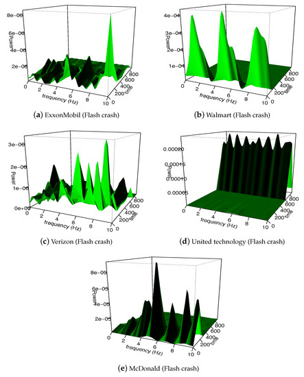
Figure 2.
3D power spectra of the financial data corresponding to the flash crash event.

Figure 3.
3D power spectra of the financial data corresponding to Citigroup and IAG stock markets.
5.2. Analysis of the Wavelet Model
In the Fourier analysis, we transformed the time domain data into the frequency domain, thereby losing the time component. With wavelets, we avoid this problem. First, wavelet analysis is performed on a short section of the time series data. The section is shifted, and the research is conducted in a new section. The process is repeated until the end of the time series.
The data from the financial crashes contain the power spectrum as the most significant value in the smaller time scale. We measure the importance of each level by evaluating the proportion of the total power (or energy) explained by each. Table 9, Table 10, Table 11, Table 12, Table 13 and Table 14 represent the proportions of the ratios of the total energy associated with each coefficient of detail to the total energy of the time series. The significant percentage value of the proportions of total energy for the flash crash events is few relative to the substantial percentage of total energy for the Lehman Brothers Collapse. Figure 4, Figure 5, Figure 6, Figure 7 and Figure 8 represent the 3-D graphical information of the energy levels corresponding to the two events. The results in Table 9, Table 10, Table 11, Table 12 and Table 13 of the Lehman Brothers bank collapse shows high energy at lower levels (level 1,2, and 3). In Table 14, this observation is consistent since the total energy for Citigroup and IAG stock markets data are high at lower levels (1, 2, and 3) compared with levels (4, 5, and 6). A previous study [3] suggested that the time series of returns captured during the Lehman Brothers event behaves like a natural tectonic earthquake; thus, this type of financial event may be predicted. Therefore, the two events, Citigroup (2009) and IAG (2011), follow the same dynamics as the Lehman Brothers.

Table 9.
Total energy for XOM stock market data.

Table 10.
Total energy for WMT stock market data.

Table 11.
Total energy for VZ stock market data.

Table 12.
Total energy for UTX stock market data.

Table 13.
Total energy for MCD stock market data.

Table 14.
Total energy for Citigroup and IAG stock markets data.
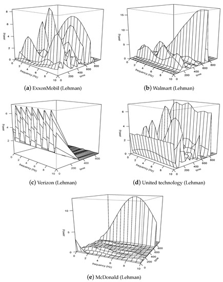
Figure 4.
The energy levels of the financial data corresponding to the Lehman Brothers collapse.
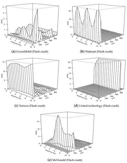
Figure 5.
The energy levels of financial data corresponding to the flash crash event.
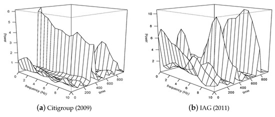
Figure 6.
The energy levels of the financial data corresponding to Citigroup and IAG stock markets.
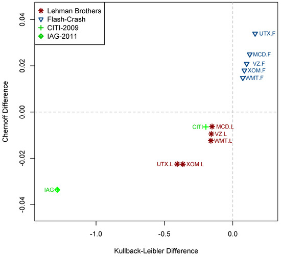
Figure 7.
Classification (by quadrant) of Lehman Brothers collapse and flash crash event using the Chernoff and Kullback–Leibler differences.
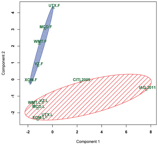
Figure 8.
Clustering results for the Lehman Brothers collapse, flash crash event, Citigroup (2009), and IAG (2011) stock data based on symmetric divergence using the PAM algorithm.
5.3. Discriminant Analysis Using KL and Chernoff Distances
Based on their frequency domain, we used the KL and Chernoff distance techniques on the Lehman Brothers collapse and flash crash event. An important feature of these techniques is that they measure the similarity of two statistical samples or populations. We then optimized the Chernoff coefficient, , to estimate the maximum value of Chernoff disparity. The KL and Chernoff distances of Citigroup’s (2009) stock market are obtained as −0.106 and −0.006, respectively. Similarly, KL and Chernoff distances of the IAG (2011) stock market are obtained as −1.283 and −0.033, respectively. Table 15 shows that the Lehman Brothers collapse has negative KL and Chernoff distances, and the flash crash has positive KL and Chernoff distances. Thus, we have correctly discriminated between the two events. Similarly, in Table 16, we observe that Citigroup (2009) and IAG (2011) have negative KL and Chernoff distances. Figure 7 shows the classification of the Lehman Brothers collapse and flash crash events using the Chernoff differences along with the KL differences. Clearly, the points in the first quadrant are classified as flash-Crash events, and the points in the third quadrant are classified as Lehman Brothers collapse. So the events of Citigroup from 2009 and IAG from 2011 have the same characteristics as the Lehman Brothers collapse event.

Table 15.
Discriminant scores for Lehman Brothers collapse and flash crash event.

Table 16.
Discriminant scores for Citigroup in 2009 and IAG stock in 2011.
5.4. Clustering Analysis
We used the partitioning around medoids (PAM) algorithm to cluster the Lehman Brothers collapse and flash crash event and their effects. We also selected the data of Citigroup (2009) to see whether the market data of this year was influenced by the crash of Lehman Brothers collapse (2008) and also verify if the IAG stock (2011) was affected by the flash crash event (2010). In Figure 8, the triangle symbols indicate the flash crash event classification, and the symbols of circles indicate the Lehman Brothers collapse classification. The figure shows that the stocks from Citigroup (2009) and IAG (2011) have the same dynamics as the Lehman Brothers collapse since they are in the same ellipse.
6. Conclusions
In this work, we studied four classification techniques: dynamic Fourier transform, wavelet transform, discriminant analysis, and clustering algorithms, to discriminate between two sets of high-frequency financial data (the Lehman Brothers collapse and the flash crash event which occurred in 2008 and 2010, respectively).
The dynamic Fourier technique helped to characterize the spectral behavior of the data. Using the fast Fourier transform, we converted the time domain data into the frequency domain by losing the time resolution and explained the power spectrum of the data. In the wavelet methodology, we analyzed the power level of the high-frequency data without losing the time information. The wavelet technique is localized in the frequency and time domain. On the other hand, this paper’s discriminant and clustering techniques measured the similarity of two statistical samples to compute the spectral matrices between the two financial events.
An essential feature of this work is that the four techniques used in this paper follow a stationary process. We then determined the stationarity by computing some unit root tests discussed in Section 4.
The results obtained in this study reinforce and validate the previous results obtained in [3], where the authors concluded that the Lehman Brothers collapse and the flash crash event could be distinguished based on the dynamics of the time series. For example, the flash crash event was an event whose dynamics are attributed to the complexity of modern equity market microstructures. The Lehman Brothers event, on the other hand, behaved like a natural tectonic earthquake. Thus, this type of financial event may be predicted [3].
We also selected two high-frequency stock market data, Citigroup from 2009 and IAG from 2011, to study their dynamics about the Lehman Brothers collapse and flash crash event. The results suggest that the two events, Citigroup (2009) and IAG (2011), behave like the Lehman Brothers collapse. Hence, they are predictable. We found similar results with all classification methodologies. The four techniques discussed in this work can discriminate between any high-frequency time series. The main difficulty of this work was fitting the models to the data. This is because the data contain financial crashes, i.e., assets suddenly lose a large part of their nominal value. The methodologies used in this paper can identify crashes’ strengths and help practitioners and researchers make informed decisions in the financial market before and after crashes.
Author Contributions
O.K.T. and M.C.M. contributed to the supervision and project administration, O.K.T., M.C.M. and M.P.B.-V. contributed to the conceptualization and methodology, and I.F. contributed to the data curation. O.K.T. and M.A.M.B. contributed to the formal analysis, visualization, and original draft preparation. All authors have read and approved the final manuscript.
Funding
This research received no external funding.
Institutional Review Board Statement
Not applicable.
Informed Consent Statement
Not applicable.
Data Availability Statement
The data supporting this study’s findings are available from the corresponding author upon reasonable request for replication purposes. For further research development, the researchers would need an active subscription to Refinitiv Data (https://www.refinitiv.com/en/financial-data/market-data/tick-history (accessed on 15 December 2022)).
Conflicts of Interest
The authors declare no conflict of interest.
References
- Luhby, T. American’s Wealth Drops 1.3 Trillion. CNNMoney.com. 11 June 2009. Available online: https://money.cnn.com/2009/06/11/news/economy/Americans_wealth_drops/ (accessed on 15 December 2022).
- Tweneboah, O.K. Applications Of Ornstein-Uhlenbeck Type Stochastic Differential Equations. Ph.D. Theses, University of Texas at El Paso, El Paso, TX, USA, 2020. Available online: https://scholarworks.utep.edu/open_etd/3052 (accessed on 15 December 2022).
- Beccar-Varela, M.P.; Mariani, M.C.; Tweneboah, O.K.; Florescu, I. Analysis of the Lehman brothers collapse and the Flash Crash event by applying wavelets methodologies. Phys. A Stat. Mech. Appl. 2017, 474, 162–171. [Google Scholar] [CrossRef]
- Mariani, M.C.; Bhuiyan, M.A.M.; Tweneboah, O.K.; Beccar-Varela, M.P.; Florescu, I. Analysis of stock market data by using Dynamic Fourier and Wavelets techniques. Phys. A Stat. Mech. Appl. 2020, 537, 122785. [Google Scholar] [CrossRef]
- Vuorenmaa, T.A. A wavelet analysis of scaling laws and long-memory in stock market volatility. In Noise and Fluctuations in Econophysics and Finance; Bank of Finland Research Discussion Paper No. 27/2005; SPIE: Helsinki, Finland, 2005. [Google Scholar]
- Dajcman, S. Interdependence between some major European stock markets-A wavelet lead/lag analysis. Prague Econ. Pap. 2013, 22, 28–49. [Google Scholar] [CrossRef]
- Shumway, R.H.; Stoffer, D.S. Time Series Analysis and Its Applications with R Examples; Springer: Berlin/Heidelberg, Germany, 2010. [Google Scholar]
- Cryer, J.D.; Chan, K.S. Time Series Analysis with its Applications in R; Springer: Berlin/Heidelberg, Germany, 2008; pp. 351–367. [Google Scholar]
- Kaufman, L.; Rousseeuw, P.J. Finding Groups in Data: An Introduction to Cluster Analysis; John Wiley & Sons: Hoboken, NJ, USA, 1990; pp. 68–125. [Google Scholar]
- Wiggins, R.Z.; Piontek, T.; Metrick, A. The Lehman Brothers Bankruptcy A: Overview. J. Financ. Cris. 2019, 1, 39–62. [Google Scholar] [CrossRef]
- NANEX. 2010 Flash Crash Analysis, Final Conclusion. 6 May 2010. Available online: http://www.nanex.net/FlashCrashFinal/FlashCrashAnalysis_Theory.html (accessed on 15 December 2022).
- Kwiatkowski, D.; Phillips, P.C.B.; Schmidt, P.; Shin, Y. Testing the Null Hypothesis of Stationarity against the Alternative of a Unit Root. J. Econom. 1992, 54, 159–178. [Google Scholar] [CrossRef]
Disclaimer/Publisher’s Note: The statements, opinions and data contained in all publications are solely those of the individual author(s) and contributor(s) and not of MDPI and/or the editor(s). MDPI and/or the editor(s) disclaim responsibility for any injury to people or property resulting from any ideas, methods, instructions or products referred to in the content. |
© 2023 by the authors. Licensee MDPI, Basel, Switzerland. This article is an open access article distributed under the terms and conditions of the Creative Commons Attribution (CC BY) license (https://creativecommons.org/licenses/by/4.0/).