Analysis of $\mathbf{ℝ}\mathbf{=}\mathit{P}[\mathit{Y}\mathbf{<}\mathit{X}\mathbf{<}\mathit{Z}\mathbf{]}$ Using Ranked Set Sampling for a Generalized Inverse Exponential Model

Abstract

In many real-world situations, systems frequently fail due to demanding operating conditions. In particular, when systems reach their lowest, highest, or both extremes operating conditions, they usually fail to accomplish their intended functions. This study considers estimating the stress–strength reliability, for a component with a strength ($X$) that is independent of the opposing lower bound stress ($Y$) and upper bound stress ($Z$). We assumed that the strength and stress random variables followed a generalized inverse exponential distribution with different shape parameters. Under ranked set sampling (RSS) and simple random sampling (SRS) designs, we obtained four reliability estimators using the maximum likelihood method. The first and second reliability estimators were deduced when the sample data of the strength and stress distributions used the sample design (RSS/SRS). The third reliability estimator was determined when the sample data for $Y$ and $Z$ were received from the RSS and the sample data for $X$ were taken from the SRS. The fourth reliability estimator was derived when the sample data of $Y$ and $Z$ were selected from the SRS, while the sample data of $X$ were taken from the RSS. The accuracy of the suggested estimators was compared using a comprehensive computer simulation. Lastly, three real data sets were used to determine the reliability.

1. Introduction

In reliability theory, a component’s life is defined using stress–strength (SS) models, which include a random strength ($X$) exposed to a random stress (Y). When the stress level applied to a component exceeds its strength level, the component fails immediately. The basic SS model $R=P\left(Y<X\right)$ was first considered in [1]. Another important SS model is the type of $ℝ=\hspace{0.17em}P[Y<X<Z]$, which illustrates the situation where a strength $X$ should not only be larger than a stress $Y$ but also smaller than a stress $Z.$ As a concrete example, it is common that electronic devices are unable to function at excessively low and high temperatures, and the SS model becomes of interest to model this phenomenon. Recently, a lot of effort has been put into estimating SS models for different stress and strength distributions. The maximum likelihood estimator (MLE) and uniform minimum unbiased estimator for $ℝ$ were developed in [2]. Ref. [3] constructed estimators of $ℝ$, where $X$, $Y$ and $Z$ were all random variables that follow the normal distribution. Ref. [4] investigated an estimator of $ℝ$, where the stresses and strength were exponentially distributed. Ref. [5] offered an estimate of $ℝ$ for the Weibull distribution in the presence of outliers. The estimation of $ℝ$ when the strength and stress random variables follow the Dagum distribution was explored in [6,7]. Ref. [8] studied the reliability estimator of $ℝ=\hspace{0.17em}P[Y<X<Z]$ from the inverse Rayleigh distribution using data outliers. Ref. [9] looked into some classical estimation methods, assuming an inverse Rayleigh distribution for both stresses and strength random variables. Ref. [10] dealt with the SS parameter, when X, $Y$ and $Z$ had three independent Kumaraswamy distributions.

On the other hand, an efficient and successful alternative for simple random sampling (SRS) is ranked set sampling (RSS). When the sampling units are expensive and challenging to measure, this is frequently used to obtain samples that are more representative of the underlying population, simple and inexpensive to order in accordance with the variable of interest. Numerous studies have been conducted on alterations of the RSS procedure. The reader can find further information on the RSS system in, for example, [11,12,13,14]. Several authors have performed studies concerning the reliability estimation of SS models under the RSS, including [15,16,17,18,19].

To the best of our knowledge, there have been no papers published that employed RSS design to assess the reliability parameter of type $ℝ=\hspace{0.17em}P[Y<X<Z]$ in the literature. Thus, our motivation here was to assess the reliability estimator of $ℝ$ using the maximum likelihood procedure, given that stresses and strength are three independent random variables that follow the generalized inverse exponential distribution (GIED) with distinct shape parameters and a similar scale parameter. The reliability estimator of $ℝ$ is discussed in the following cases:

(i)

The first and second reliability estimators of $ℝ=\hspace{0.17em}P[Y<X<Z]$ were derived when X, $Y$ and Z are independent random variables with the same sampling design (RSS or SRS).

(ii)

The third estimator of $ℝ$ was constructed when the observed stress random variables $Y$ and $Z$ came from the RSS and the data for strength random variable $X$ came from the SRS.

(iii)

Finally, we obtained the fourth estimator, assuming that the observed samples of $Y$ and $Z$ came from the SRS design, and the data of X came from the RSS scheme.

Furthermore, a simulation study employing iterative methods, such as the Newton–Raphson algorithm, was used to compare the performance of various estimators, based on certain accuracy measures. Finally, real datasets were analyzed for illustrative purposes.

The rest of this article is organized as follows: A description of the RSS scheme is given in Section 2. Section 3 contains the exact formulation of $ℝ$ based on the GIED. The MLE of $ℝ$ is derived using the SRS and RSS in Section 4 and Section 5, respectively. Section 6 gives the reliability estimator of $ℝ$, assuming the observed samples of $Y$ and $Z$ come from the RSS, and the selected samples of $X$ come from the SRS. Section 7 provides the reliability estimator of $ℝ$, assuming the collected samples of $Y$ and $Z$ are selected from the RSS, and the selected samples of $X$ are taken from the SRS. Section 8 contains a simulation study and its results. Three real data sets are provided in Section 9, to examine the behavior of the proposed estimators. Finally, in Section 10, we bring the paper to a close.

2. Structure of Ranked Set Sampling

In contrast to the same number of observations collected from SRS, the goal of RSS design is to collect observations from a population that are more likely to cover the entire range of values in the population. RSS has numerous applications in science, particularly in environmental and ecological studies, where the main focus is on cost-effective and efficient sampling techniques. Ref. [20] pioneered the theory of RSS in cases where the quantification of sample items is too expensive or impossible, but the variable to be monitored may be ranked more readily and cheaply than measured. The authors claimed that using RSS to estimate a population’s mean is far more useful and preferable to using SRS. Ref. [21] demonstrated mathematically that the RSS mean estimator outperformed SRS.

2.1. RSS Description

The steps listed below provide an explanation of RSS

• Randomly select n² units from the targeted population and arrange them into n sets, each of size n. We denote the result by

  $$\left(\begin{array}{llll}{X}_{11}& X_{12}& \dots & X_{1n}\\ X_{21}& X_{22}& \dots & X_{2n}\\ ⋮& ⋮& \ddots & ⋮\\ X_{n1}& X_{n2}& \dots & X_{nn}\end{array}\right)$$

2

The n units within each set are sorted according to the variable of interest using visual examination or any other inexpensive approach. The number of units, n, in each row is called the set size. The result is presented as

$$\left(\begin{array}{llll}{X}_{(1)1}& X_{(2)1}& \dots & X_{(n)1}\\ X_{(1)2}& X_{(2)2}& \dots & X_{(n)2}\\ ⋮& ⋮& \ddots & ⋮\\ X_{(1)n}& X_{(2)n}& \dots & X_{(n)n}\end{array}\right) \mathrm{which} \mathrm{will} \mathrm{be} \mathrm{one} \mathrm{cycle}.$$

3

After ranking all sets, the smallest ranked unit is quantified from the first set. Similarly, the second smallest ranked unit is quantified from the second set, and the procedure continues until the largest ranked unit is quantified from the last set. As a result, the RSS associated with this cycle will be $\left(X_{\left(1\right)1};X_{\left(2\right)2}; \dots ;X_{\left(n\right)n}\right)$. The measured observations $\left(X_{\left(1\right)1};X_{\left(2\right)2}; \dots ;X_{\left(n\right)n}\right)$ constitute a balanced RSS of size n, where the descriptor “balanced” refers to the fact that we have collected one judgment order statistic (OS) for each of the ranks 1, 2, …,n.

4

Repeat steps (1)–(3) d times (cycles) until obtaining a sample of size $n^{\ast \ast }=nd,$ where n is the set size. The RSS of sample size $n^{\ast \ast }$, will be $\{X_{(i)}{}_{ia},i=1,2,\dots n,\hspace{0.17em}\hspace{0.17em}a=1,\dots ,d\}.$ It should be noted that we use the notations $X_{ia}$, rather than $X_{(i)}{}_{ia},$ for the sake of brevity, then the RSS can be written as $\{X_{ia},i=1,2,\dots n,\hspace{0.17em}\hspace{0.17em}a=1,\dots ,d\}.$

If the judgment ranking is perfect, the probability density function (PDF) of ith OS $X_{ia}$ is given by

$$f_{ia}(x_{ia})=\frac{n!}{(i-1)!(n-i)!}{\left[F_X(x_{ia})\right]}^{i-1}{f}_X(x_{ia}){\left[1-F_X(x_{ia})\right]}^{n-i},\hspace{0.17em}\hspace{0.17em}\hspace{0.17em}\hspace{0.17em}-\infty \hspace{0.17em}<x_{ia}<\infty .$$

(1)

2.2. Choices of Set Size and Cycle Number

Any RSS procedure’s performance is highly dependent on the set size. Each measured RSS observation uses additional information derived from its ranking compared to n − 1 other units in the population for a given set size n. Perfect rankings is preferable to use a set size n that is as large as is economically feasible, given the resources at our disposal. In order to achieve ideal rankings, we would like to increase the set size n to the maximum level that is economically feasible given the resources at our disposal. It is also evident that the likelihood of ranking errors increases with the set size, i.e., the larger n is, the more probable ranking errors are to occur. As a result, in order to best choose the set size n, one must be able to estimate the probability of imperfect rankings and evaluate how they will affect the RSS statistical methods [22]. Ref. [20] suggested that set sizes larger than five would probably not improve the efficiency of the RSS very much because set sizes this large would likely result in too many ranking errors.

3. Description of the Model

In this section, we provide an expression for system reliability $ℝ=\hspace{0.17em}P[Y<X<Z],$ assuming that the random variables $X$, $Y$ and $Z$ follow the GIED with different shape parameters. For this, we need a short review of the GIED.

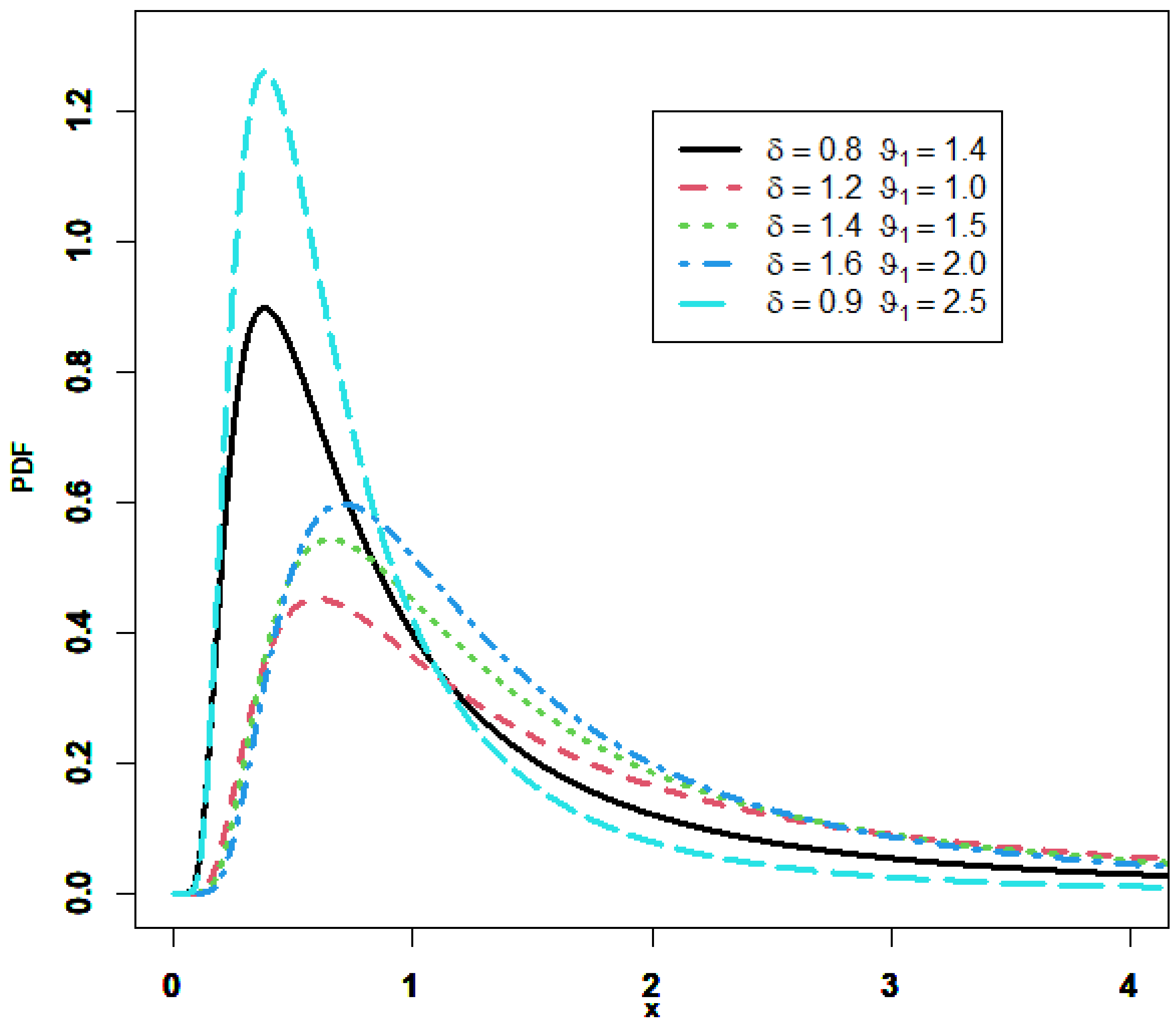
Inverted distributions were created to address certain laws in several widely used distributions in a variety of fields, including the biological sciences, survival research, and engineering sciences. Different aspects of the behavior of the related probability functions may be seen in these distributions. Ref. [23] proposed a useful two-parameter extension of the inverted exponential distribution, known as the GIED. They mentioned that the GIED offers a superior fit than the gamma, Weibull, generalized exponential, and inverted exponential distributions in a number of situations. The probability density function (PDF) of the GIED with the shape parameter ${\vartheta }_1$ and the scale parameter $\delta$ is given by

$$f_X(x)=\frac{\delta {\vartheta }_1}{x^2}{e}^{-(\delta /x)}{\left(1-e^{-(\delta /x)}\right)}^{{\vartheta }_1-1};\hspace{0.17em}\hspace{0.17em}\hspace{0.17em}\hspace{0.17em}\hspace{0.17em}\hspace{0.17em}\hspace{0.17em}\hspace{0.17em}\hspace{0.17em}\hspace{0.17em}\hspace{0.17em}x,\delta ,{\vartheta }_1>0.$$

(2)

The cumulative distribution function (CDF) of the GIED is given by

$$F_X(x)=1-{\left(1-e^{-(\delta /x)}\right)}^{{\vartheta }_1};\hspace{0.17em}\hspace{0.17em}\hspace{0.17em}\hspace{0.17em}\hspace{0.17em}\hspace{0.17em}\hspace{0.17em}\hspace{0.17em}\hspace{0.17em}\hspace{0.17em}\hspace{0.17em}x,\delta ,{\vartheta }_1>0.$$

(3)

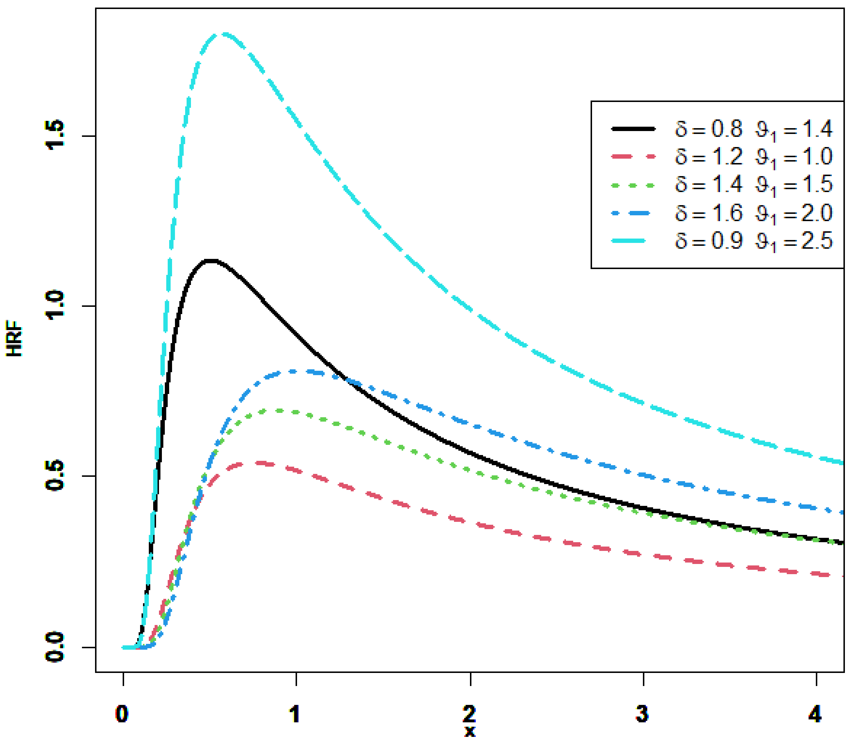
The hazard rate function (HRF) of the GIED is given by

$$H_X(x)=\frac{\delta {\vartheta }_1}{x^2\left(1-e^{-(\delta /x)}\right)}{e}^{-(\delta /x)};\hspace{0.17em}\hspace{0.17em}\hspace{0.17em}\hspace{0.17em}\hspace{0.17em}\hspace{0.17em}\hspace{0.17em}\hspace{0.17em}\hspace{0.17em}\hspace{0.17em}\hspace{0.17em}x,\delta ,{\vartheta }_1>0.$$

(4)

Ref. [24] mentioned that the GIED is a special case of the exponentiated Fréchet distribution. Due to the CDF closed shape, the GIED is frequently used in studies, including accelerated life testing, horse racing, grocery store lines, sea currents, wind speeds, and a variety of other topics (see [25]). Figure 1 displays the different forms achieved with the PDF. We can observe that it is right-skewed and unimodal. Depending on the distribution’s shape parameter, the HRF of the GIED increases then decreases, in an upside-down shape, but it is not constant, as illustrated in Figure 2.

Figure 1. Plots of the PDF of the GIED for different parameter values.

Figure 2. Plots of the HRF for the GIED for different parameter values.

Researchers have made various contributions and applications in various fields using different types of data relevant to the GIED. For example, in reliability studies, Ref. [26] explored reliability estimates for the GIED in progressively censored samples. A parameter estimation for the GIED using different methods and schemes was provided in [27,28]. In statistical quality control, Ref. [29] discussed a two-stage acceptance sampling plan for the GIED. Under hybrid random censoring, Ref. [30] presented the Bayesian inference on the GIED parameters. In life testing experiments, Ref. [31] investigated the estimation and prediction for the GIED based on progressively censored first-failure data. Ref. [32] looked into Bayesian estimators and SS reliability (SSR) estimators related to the GIED, based on progressively censored first-failure data. Ref. [33] investigated parameter estimation in the context of the GIED using an adaptive progressive hybrid censoring scheme. Ref. [34] investigated the reliability of Bayesian analysis in multicomponent SS for the GIED using upper record data. Ref. [35] investigated a competing risks model where the lifetimes were independent random variables that followed the GIED.

To obtain SSR, $ℝ=\hspace{0.17em}P[Y<X<Z],$ let the strength $X$~GIED$(\delta ,{\vartheta }_1),$ the stress $Y$~GIED$(\delta ,{\vartheta }_2)$, and stress $Z$~GIED$(\delta ,{\vartheta }_3)$, where $X$, $Y$ and $Z$ are independent random variables (the tilde notation meaning “follows the distribution”). According to Ref. [3], the reliability formula of the SS model of $ℝ=\hspace{0.17em}P[Y<X<Z],$ takes the following form:

$$ℝ=\hspace{0.17em}P[Y<X<Z]={\int }_{-\infty }^{\infty }{G}_Y\left(x\right){\overline{H}}_Z\left(x\right)d{F}_X\left(x\right) ,$$

(5)

where $F_X(x)$ is the CDF of $X$, $G_Y(x)$ is the CDF of $Y$ at x, and ${\overline{H}}_Z(x)$ is the survival function of $Z$ at x. Hence, $ℝ=\hspace{0.17em}P[Y<X<Z],$ is derived as follows:

$$ℝ=\hspace{0.17em}P[Y<X<Z]=\delta {\vartheta }_1{\int }_0^{\infty }{\left(1-e^{-(\delta /x)}\right)}^{{\vartheta }_3}\left[1-{\left(1-e^{-(\delta /x)}\right)}^{{\vartheta }_2}\right] x^{-2}{e}^{-(\delta /x)}{\left(1-e^{-(\delta /x)}\right)}^{{\vartheta }_1-1}dx.$$

(6)

Let $y=e^{-(\delta /x)}\to dy=\delta x^{-2}{e}^{-(\delta /x)}dx,$ then $ℝ$ obtains the following ratio-parametric formula:

$$ℝ\hspace{0.17em}=\frac{{\vartheta }_1}{{\vartheta }_1+{\vartheta }_3}-\frac{{\vartheta }_1}{{\vartheta }_1+{\vartheta }_2+{\vartheta }_3}=\frac{{\vartheta }_1{\vartheta }_2}{({\vartheta }_1+{\vartheta }_3)({\vartheta }_1+{\vartheta }_2+{\vartheta }_3)}.$$

(7)

It is worth noting that the SS parameter in (7) is dependent on the parameters ${\vartheta }_1,{\vartheta }_2$ and ${\vartheta }_3.$

4. Estimator of ${\mathbf{ℝ}}_{\mathbf{1}}\mathbf{=}\mathit{P}\mathbf{[}{\mathit{Y}}_{\mathit{S}\mathit{R}\mathit{S}}\mathbf{<}{\mathit{X}}_{\mathit{S}\mathit{R}\mathit{S}}\mathbf{<}{\mathit{Z}}_{\mathit{S}\mathit{R}\mathit{S}}\mathbf{]}$

In this section, the MLE of ${ℝ}_1$, say ${\widehat{ℝ}}_1,$ is discussed, where $X_1,X_2,\dots ,X_{n^{\ast }{}_1},$ $Y_1,Y_2,\dots ,Y_{n^{\ast }{}_2}$ and $Z_1,Z_2,\dots ,Z_{n^{\ast }{}_3}$ are independent random variables of the GIED with parameters $(\delta ,{\vartheta }_1),$ $(\delta ,{\vartheta }_2)$, and $(\delta ,{\vartheta }_3),$ respectively, under the SRS. To calculate the MLE of ${ℝ}_1$, we first obtain the MLE of ${\vartheta }_1,{\vartheta }_2,{\vartheta }_3$, and $\delta .$ The joint log likelihood function of the random samples $x_1,x_2,\dots ,x_{n^{\ast }{}_1},$$y_1,y_2,\dots ,y_{n^{\ast }{}_2}$, and $z_1,z_2,\dots ,z_{n^{\ast }{}_3}$ is

$$\begin{array}{c}\ln {\ell }_1=n^{\ast }{}_1\ln {\vartheta }_1+n^{\ast }{}_2\ln {\vartheta }_2+n^{\ast }{}_3\ln {\vartheta }_3+(n^{\ast }{}_1+n^{\ast }{}_2+n^{\ast }{}_3)\ln \delta -2\left[{\displaystyle \sum _{i_1=1}^{n^{\ast }{}_1}\ln }\hspace{0.17em}{x}_{i_1}+{\displaystyle \sum _{i_2=1}^{n^{\ast }{}_2}\ln }\hspace{0.17em}{y}_{i_2}+{\displaystyle \sum _{i_3=1}^{n^{\ast }{}_3}\ln }\hspace{0.17em}{z}_{i_3}\right]\\ -{\displaystyle \sum _{i_1=1}^{n^{\ast }{}_1}\frac{\delta }{\hspace{0.17em}{x}_{i_1}}}-{\displaystyle \sum _{i_2=1}^{n^{\ast }{}_2}\frac{\delta }{\hspace{0.17em}{y}_{i_2}}}\hspace{0.17em}-{\displaystyle \sum _{i_3=1}^{n^{\ast }{}_3}\frac{\delta }{\hspace{0.17em}{z}_{i_3}}}+({\vartheta }_1-1){\displaystyle \sum _{i_1=1}^{n^{\ast }{}_1}{A}_{{}^{i_1}}(\delta )}+({\vartheta }_2-1){\displaystyle \sum _{i_2=1}^{n^{\ast }{}_2}{A}_{i_2}(\delta )}+({\vartheta }_3-1){\displaystyle \sum _{i_3=1}^{n^{\ast }{}_3}{A}_{i_3}(\delta )},\end{array}$$

(8)

where $A_{i_1}(\delta )=\ln \left(1-e^{-\left(\delta /x_{i{\hspace{0.17em}}_1}\right)}\right),$$A_{i_2}(\delta )=\ln \left(1-e^{-\left(\delta /y_{i{\hspace{0.17em}}_2}\right)}\right),$ $A_{i_3}(\delta )=\ln \left(1-e^{-\left(\delta /z_{i{\hspace{0.17em}}_3}\right)}\right).$

The equations below are determined using differentiation (Equation (8)) linked to the population parameters.

$$\frac{\partial \ln {\ell }_1}{\partial {\vartheta }_1}=\frac{n^{\ast }{}_1}{{\vartheta }_1}+{\displaystyle \sum _{i_1=1}^{n^{\ast }{}_1}{A}_{i_1}(\delta )},$$

(9)

$$\frac{\partial \ln {\ell }_1}{\partial {\vartheta }_2}=\frac{n^{\ast }{}_2}{{\vartheta }_2}+{\displaystyle \sum _{i_2=1}^{n^{\ast }{}_2}{A}_{i_2}(\delta )},$$

(10)

$$\frac{\partial \ln {\ell }_1}{\partial {\vartheta }_3}=\frac{n^{\ast }{}_3}{{\vartheta }_3}+{\displaystyle \sum _{i_3=1}^{n^{\ast }{}_3}{A}_{i_3}(\delta )},$$

(11)

$$\begin{array}{ll}\frac{\partial \ln {\ell }_1}{\partial \delta }=& \frac{(n^{\ast }{}_1+n^{\ast }{}_2+n^{\ast }{}_3)}{\delta }-\left[{\displaystyle \sum _{i_1=1}^{n^{\ast }{}_1}(x_{i_1}}{)}^{-1}+{\displaystyle \sum _{i_2=1}^{n^{\ast }{}_2}{(y_{i_2})}^{-1}}+{\displaystyle \sum _{i_3=1}^{n^{\ast }{}_3}{(z_{i_3})}^{-1}}\right]+{\displaystyle \sum _{i_1=1}^{n^{\ast }{}_1}({\vartheta }_1-1)A_{i_1}^{\prime }(\delta )}+\hspace{0.17em}{\displaystyle \sum _{i_2=1}^{n^{\ast }{}_2}({\vartheta }_2-1)A_{i_2}^{\prime }(\delta )}\\ & +{\displaystyle \sum _{i_3=1}^{n^{\ast }{}_3}({\vartheta }_3-1)A_{i_3}^{\prime }(\delta )},\end{array}$$

(12)

where $A_{i_1}^{\prime }(\delta )=\frac{\partial A_{i_1}(\delta )}{\partial \delta }={\left[x_{i_1}\left(e^{\left(\delta /x_{i_1}\right)}-1\right)\right]}^{-1},$$A_{i_2}^{\prime }(\delta )=\frac{\partial A_{i_2}(\delta )}{\partial \delta }={\left\{y_{i_2}\left(e^{\left(\delta /y_{{}^{i_2}}\right)}-1\right)\right\}}^{-1}$ and $A_{i_3}^{\prime }(\delta )=\frac{\partial A_{i_3}(\delta )}{\partial \delta }={\left\{z_{i_3}\left(e^{\left(\delta /z_{{}^{i_3}}\right)}-1\right)\right\}}^{-1}.$

Put (9)–(11) with zero to yield the MLEs of ${\vartheta }_1,{\vartheta }_2$ and ${\vartheta }_3$ as a function of $\delta .$ They are explicated as:

$${\widehat{\vartheta }}_1(\delta )=\frac{-n^{\ast }{}_1}{{\displaystyle \sum _{i_1=1}^{n^{\ast }{}_1}{A}_{i_1}(\delta )}}, {\widehat{\vartheta }}_2(\delta )=\frac{-n^{\ast }{}_2}{{\displaystyle \sum _{i_2=1}^{n^{\ast }{}_2}{A}_{i_2}(\delta )}}, {\widehat{\vartheta }}_3(\delta )=\frac{-n^{\ast }{}_3}{{\displaystyle \sum _{i_3=1}^{n^{\ast }{}_3}{A}_{i_3}(\delta )}}$$

(13)

Set (13) in (12) and equate with zero, which leads to the following equation:

$$\frac{n^{\ast }{}_1+n^{\ast }{}_2+n^{\ast }{}_3}{\left[{\displaystyle \sum _{i_1=1}^{n^{\ast }{}_1}\frac{1}{x_{i_1}}+}{\displaystyle \sum _{i_2=1}^{n^{\ast }{}_2}\frac{1}{y_{i_2}}+{\displaystyle \sum _{i_3=1}^{n^{\ast }{}_3}\frac{1}{z_{i_3}}}}\right]+\left(\frac{n^{\ast }{}_1}{{\displaystyle \sum _{i_1=1}^{n^{\ast }{}_1}{A}_{i_1}(\widehat{\delta })}}+1\right)\left({\displaystyle \sum _{i_1=1}^{n^{\ast }{}_1}{A}_{i_1}^{\prime }(\widehat{\delta })}\right)+\left(\frac{n^{\ast }{}_2}{{\displaystyle \sum _{i_2=1}^{n^{\ast }{}_2}{A}_{i_2}(\widehat{\delta })}}+1\right)\left({\displaystyle \sum _{i_2=1}^{n^{\ast }{}_2}{A}_{i_2}^{\prime }(\widehat{\delta })}\right)+\left(\frac{n^{\ast }{}_3}{{\displaystyle \sum _{i_3=1}^{n^{\ast }{}_3}{A}_{i_3}(\widehat{\delta })}}+1\right)\left({\displaystyle \sum _{i_3=1}^{n^{\ast }{}_3}{A}_{i_3}^{\prime }(\widehat{\delta })}\right)}=0.$$

(14)

Using the Newton–Raphson iterative method, the MLE of $\delta$, say $\hat{\delta }$ is produced from (14). Hence, the MLEs of ${\vartheta }_1,{\vartheta }_2,$ and ${\vartheta }_3$ say ${\widehat{\vartheta }}_1,{\widehat{\vartheta }}_2,$ and ${\widehat{\vartheta }}_3,$ are yielded by inserting $\widehat{\delta }$ in (13). The SS estimator ${\widehat{ℝ}}_1$ is also provided by putting ${\widehat{\vartheta }}_1,{\widehat{\vartheta }}_2,$ and ${\widehat{\vartheta }}_3$ in (7).

5. Estimator of ${\mathbf{ℝ}}_{\mathbf{2}}\mathbf{=}\mathit{P}\mathbf{[}{\mathit{Y}}_{\mathit{R}\mathit{S}\mathit{S}}\mathbf{<}{\mathit{X}}_{\mathit{R}\mathit{S}\mathit{S}}\mathbf{<}{\mathit{Z}}_{\mathit{R}\mathit{S}\mathit{S}}\mathbf{]}$

In this section, the MLE of ${ℝ}_2$, say ${\widehat{ℝ}}_2$, is obtained where strength $X$, and stresses $Y$ and $Z$, are independent random variables that follow the GIED with parameters $(\delta ,{\vartheta }_1),$ $(\delta ,{\vartheta }_2)$, and $(\delta ,{\vartheta }_3),$ respectively, using the RSS method.

Let $X_{ka}$ represent the OS of the kth sample, k = 1, 2, …, n₁, in the ath cycle, a = 1, 2, …, d_x, $n_1^{\ast \ast }=n_1{d}_x$ from the GIED $(\delta ,{\vartheta }_1).$ Hence, the RSS of the strength $X$ for (d_x) cycle with sample size $n_1^{\ast \ast }=n_1{d}_x$, where a = 1, 2, …, d_x, and $n_1$ the set size, is represented as $X_{ka}\equiv \{X_{1a},X_{2a},\dots ,X_{n_{1}a}\}.$

Similarly, let $Y_{sb}$, be the OS of sth sample, s = 1, 2, …,n₂, in the bth cycle, b = 1, 2,…,d_y, $n_2^{\ast \ast }=n_2{d}_y$ from the GIED $(\delta ,{\vartheta }_2).$ Hence, the RSS of the stress $Y$ for (d_y) cycle with sample size $n_2^{\ast \ast }=n_2{d}_y$, where, b = 1, 2,…,d_y and $n_2$ the set size, is represented as $Y_{sb}\equiv \{Y_{1b},Y_{2b},\dots ,Y_{n_{2b}}\}.$

In addition, suppose that $Z_{tc}$ is the OS of tth sample, t = 1, 2, …,n₃, in the cth cycle, c = 1, 2, …,d_z, $n_3^{\ast \ast }=n_3{d}_z$ from the GIED $(\delta ,{\vartheta }_3).$ Hence, the RSS of the stress $Z$ for (d_z) cycle with sample size $n_3^{\ast \ast }=n_3{d}_z$, c = 1, 2, …,d_z, and $n_3$ the set size is represented as $Z_{tc}\equiv \{Z_{1c},Z_{2c},\dots ,Z_{n_{3c}}\}.$

It is worth noting that the PDFs of $X_k{}_a$, $Y_{sb}$ and $Z_{tc}$ are equivalent to the PDFs of the kth, sth, and tth OS, respectively. Based on PDF (1), the likelihood function of $X_k{}_a$, $Y_{sb}$ and $Z_{tc}$ using the RSS is given by

$$\begin{array}{ll}{\ell }_2=& {\displaystyle \prod _{a=1}^{d_x}{\displaystyle \prod _{k=1}^{n_1}\frac{C_1\delta {\vartheta }_1}{x_{{}^{ka}}^2}{e}^{(-\delta /x_{ka})}{({\mathsf{\Xi }}_1(x_{ka},\delta ))}^{{\vartheta }_1(n_1-k+1)-1}{[1-{({\mathsf{\Xi }}_1(x_{ka},\delta ))}^{{\vartheta }_1}]}^{k-1}}}\\ & \times {\displaystyle \prod _{b=1}^{d_y}{\displaystyle \prod _{s=1}^{n_2}\frac{C_2\delta {\vartheta }_2}{y_{{}^{{}_{sb}}}^2}{e}^{(-\delta /y_{{}^{{}_{sb}}})}{({\mathsf{\Xi }}_2(y_{sb},\delta ))}^{{\vartheta }_2(n_2-s+1)-1}{[1-{({\mathsf{\Xi }}_2(y_{sb},\delta ))}^{{\vartheta }_2}]}^{s-1}}}\\ & \times \hspace{0.17em}{\displaystyle \prod _{c=1}^{d_z}{\displaystyle \prod _{t=1}^{n_3}\frac{C_3\delta {\vartheta }_3}{z_{{}^{{}_{t\hspace{0.17em}c}}}^2}{e}^{(-\delta /z_{{}^{{}_{tc}}})}{({\mathsf{\Xi }}_3(z_{tc},\delta ))}^{{\vartheta }_3(n_3-t+1)-1}{[1-{({\mathsf{\Xi }}_3(z_{tc},\delta ))}^{{\vartheta }_3}]}^{t-1},}}\hspace{0.17em}\hspace{0.17em}\end{array}$$

where $C_i=\frac{n_i!}{(\Delta -1)!(n_i-\Delta )!},\hspace{0.17em}\hspace{0.17em}\hspace{0.17em}i=1,2,3;$ $\Delta \equiv (k,s,t),$ respectively, ${\mathsf{\Xi }}_1(x_{ka},\delta )=\left[1-e^{-(\delta /x_{{}_{ka}})}\right],\hspace{0.17em}$ ${\mathsf{\Xi }}_2(y_{sb},\delta )=\left[1-e^{-(\delta /y_{{}_{sb}})}\right],$ ${\mathsf{\Xi }}_3(z_{tc},\delta )=\left[1-e^{-(\delta /z_{{}_{tc}})}\right].$

The log-likelihood function, based on the RSS, is obtained as

$$\begin{array}{ll}\ln {\ell }_2& \propto n_1^{**}\ln (\delta {\vartheta }_1)-{\displaystyle \sum _{a=1}^{d_x}\left[{\displaystyle \sum _{k=1}^{n_1}\frac{\delta }{x_{ka}}-\left[{\vartheta }_1(n_1-k+1)-1\right]\ln ({\mathsf{\Xi }}_1(x_{ka},\delta ))-(k-1)\ln \left(1-{({\mathsf{\Xi }}_1(x_{ka},\delta ))}^{{\vartheta }_1}\right)}\right]}\hspace{0.17em}+n_2^{**}\ln (\delta {\vartheta }_2)\\ & -\hspace{0.17em}{\displaystyle \sum _{b=1}^{d_y}{\displaystyle \sum _{s=1}^{n_2}\frac{\delta }{y_{s\hspace{0.17em}b}}}}+{\displaystyle \sum _{b=1}^{d_y}\left\{{\displaystyle \sum _{s=1}^{n_2}\left\{\left[{\vartheta }_2(n_2-s+1)-1\right]\ln ({\mathsf{\Xi }}_2(y_{sb},\delta ))+(s-1)\ln \left(1-{({\mathsf{\Xi }}_2(y_{sb},\delta ))}^{{\vartheta }_2}\right)\right\}}\right\}+\hspace{0.17em}}{n}_3^{**}\ln (\delta {\vartheta }_3)\hspace{0.17em}\\ & -{\displaystyle \sum _{c=1}^{d_z}{\displaystyle \sum _{t=1}^{n_3}\frac{\delta }{z_{t\hspace{0.17em}c}}-\left[{\vartheta }_3(n_3-t+1)-1\right]\ln ({\mathsf{\Xi }}_3(z_{tc},\delta ))}}+\hspace{0.17em}{\displaystyle \sum _{c=1}^{d_z}{\displaystyle \sum _{t=1}^{n_3}(t-1)}}\ln \left(1-{({\mathsf{\Xi }}_3(z_{tc},\delta ))}^{{\vartheta }_3}\right).\end{array}$$

The MLEs of ${\vartheta }_1,{\vartheta }_2,{\vartheta }_3$, and $\delta$ are obtained by maximizing this function with respect to the parameters, and can be generated as follows:

$$\begin{array}{ll}\frac{\partial \ln {\ell }_2}{\partial \delta }=& \left(\frac{n^{\ast \ast }{}_1+n^{\ast \ast }{}_2+n^{\ast \ast }{}_3}{\delta }\right)-{\displaystyle \sum _{a=1}^{d_x}\left\{{\displaystyle \sum _{k=1}^{n_1}\left[\frac{1}{x_{ka}}-\frac{\left[{\vartheta }_1(n_1-k+1)-1\right]e^{-(\delta /x_{k\hspace{0.17em}a})}}{x_{ka}{\mathsf{\Xi }}_1(x_{ka},\delta )}+\frac{(k-1){\vartheta }_1{({\mathsf{\Xi }}_1(x_{ka},\delta ))}^{{\vartheta }_1-1}{e}^{-(\delta /x_{ka})}}{x_{ka}\left(1-{({\mathsf{\Xi }}_1(x_{ka},\delta ))}^{{\vartheta }_1}\right)}\right]}\right\}}\\ & -{\displaystyle \sum _{b=1}^{d_y}{\displaystyle \sum _{s=1}^{n_2}\frac{1}{y_{sb}}}}\hspace{0.17em}+{\displaystyle \sum _{b=1}^{d_y}\left\{{\displaystyle \sum _{s=1}^{n_2}\left[\frac{\left[{\vartheta }_2(n_2-s+1)-1\right]e^{-(\delta /y_{sb})}}{({\mathsf{\Xi }}_2(y_{sb},\delta ))\hspace{0.17em}{y}_{sb}}-\frac{(s-1){\vartheta }_2{({\mathsf{\Xi }}_2(y_{sb},\delta ))}^{{\vartheta }_2-1}{e}^{-(\delta /y_{sb})}}{y_{sb}\left(1-{({\mathsf{\Xi }}_2(y_{sb},\delta ))}^{{\vartheta }_2}\right)}\right]}\right\}}\\ & +{\displaystyle \sum _{c=1}^{d_z}{\displaystyle \sum _{t=1}^{n_3}\frac{\left[{\vartheta }_3(n_3-t+1)-1\right]e^{-(\delta /z_{tc})}}{{\mathsf{\Xi }}_3(z_{tc},\delta )\hspace{0.17em}{z}_{tc}}}}-{\displaystyle \sum _{c=1}^{d_z}\left\{{\displaystyle \sum _{t=1}^{n_3}\left[\frac{1}{z_{tc}}+\frac{(t-1){\vartheta }_3{({\mathsf{\Xi }}_3(z_{tc},\delta ))}^{{\vartheta }_3-1}{e}^{-(\delta /z_{tc})}}{z_{tc}\left(1-{({\mathsf{\Xi }}_3(z_{tc},\delta ))}^{{\vartheta }_3}\right)}\right]}\right\}},\end{array}$$

(15)

$$\frac{\partial \ln {\ell }_2}{\partial {\vartheta }_1}=\frac{n^{\ast \ast }{}_1}{{\vartheta }_1}+{\displaystyle \sum _{a=1}^{d_x}{\displaystyle \sum _{k=1}^{n_1}\left\{(n_1-k+1)\ln ({\mathsf{\Xi }}_1(x_{ka},\delta ))-\frac{(k-1)\ln ({\mathsf{\Xi }}_1(x_{ka},\delta ))}{\left({({\mathsf{\Xi }}_1(x_{ka},\delta ))}^{-{\vartheta }_1}-1\right)}\right\}}},$$

(16)

$$\frac{\partial \ln {\ell }_2}{\partial {\vartheta }_2}=\frac{n^{\ast \ast }{}_2}{{\vartheta }_2}+{\displaystyle \sum _{b=1}^{d_y}{\displaystyle \sum _{s=1}^{n_2}\left\{(n_2-s+1)\ln ({\mathsf{\Xi }}_2(y_{bs},\delta ))-\frac{(s-1)\ln ({\mathsf{\Xi }}_2(y_{bs},\delta ))}{\left({({\mathsf{\Xi }}_2(y_{bs},\delta ))}^{-{\vartheta }_2}-1\right)}\right\}}},$$

(17)

$$\frac{\partial \ln {\ell }_2}{\partial {\vartheta }_3}=\frac{n^{\ast \ast }{}_3}{{\vartheta }_3}+{\displaystyle \sum _{c=1}^{d_z}{\displaystyle \sum _{t=1}^{n_3}\left\{(n_3-t+1)\ln ({\mathsf{\Xi }}_3(z_{ct},\delta ))-\frac{(t-1)\ln ({\mathsf{\Xi }}_3(z_{tc},\delta ))}{\left({({\mathsf{\Xi }}_3(z_{ct},\delta ))}^{-{\vartheta }_3}-1\right)}\right\}}}.$$

(18)

Thus, the MLEs of $\delta$, ${\vartheta }_1$, ${\vartheta }_2$, and ${\vartheta }_3$ are obtained by placing (15)–(18) to zero and solving numerically with an iterative technique, such as the Newton–Raphson algorithm; we obtain ${\widehat{ℝ}}_2$ by putting these MLEs in (7).

6. Estimator of ${\mathbf{ℝ}}_{\mathbf{3}}\mathbf{=}\mathit{P}\mathbf{[}{\mathit{Y}}_{\mathit{R}\mathit{S}\mathit{S}}\mathbf{<}{\mathit{X}}_{\mathit{S}\mathit{R}\mathit{S}}\mathbf{<}{\mathit{Z}}_{\mathit{R}\mathit{S}\mathit{S}}\mathbf{]}$

In this section, the MLE, ${\widehat{ℝ}}_3$, is determined when the strength data of $X$ are taken from the SRS, while the stresses data of $Y$ and Z are taken from the RSS design. We assume that $X$~GIED$(\delta ,{\vartheta }_1),$$Y$~GIED$(\delta ,{\vartheta }_2),$ and $Z$~GIED$(\delta ,{\vartheta }_3),$ and that $X$, $Y$ and $Z$ are independent.

Let $X_1,X_2,\dots ,X_{n^{\ast }{}_1}$ be a SRS observed from the GIED $(\delta ,{\vartheta }_1).$ Let $Y_{sb}$, be the OS of sth sample, s = 1, 2, …,n₂, in the bth cycle, b = 1, 2, …,d_y, with sample size $n_2^{\ast \ast }=n_2{d}_y,$ from the GIED $(\delta ,{\vartheta }_2).$ In addition, suppose that Z_tc is the OS of the tth sample, t = 1, 2, …,n₃, in the cth cycle, c = 1, 2, …,d_z, with sample size $n_3^{\ast \ast }=n_3{d}_z,$ from the GIED $(\delta ,{\vartheta }_3).$ The likelihood function ${\ell }_3$ in this case is as follows:

$$\begin{array}{ll}{\ell }_3=& {\displaystyle \prod _{i_1=1}^{n^{\ast }{}_1}\frac{\delta {\vartheta }_1}{x_{i_1}^2}}{e}^{{-(\delta /x}_{i_1})}{\left(1-e^{{-(\delta /x}_{i_1})}\right)}^{{\vartheta }_1-1}\\ & \times {\displaystyle \prod _{b=1}^{d_y}{\displaystyle \prod _{s=1}^{n_2}\frac{C_2\delta {\vartheta }_2}{y_{{}^{{}_{sb}}}^2}{e}^{(-\delta /y_{{}^{{}_{sb}}})}{({\mathsf{\Xi }}_2(y_{sb},\delta ))}^{{\vartheta }_2(n_2-s+1)-1}{[1-{({\mathsf{\Xi }}_2(y_{sb},\delta ))}^{{\vartheta }_2}]}^{s-1}}}\\ & \times \hspace{0.17em}{\displaystyle \prod _{c=1}^{d_z}{\displaystyle \prod _{t=1}^{n_3}\frac{C_3\delta {\vartheta }_3}{z_{{}^{{}_{t\hspace{0.17em}c}}}^2}{e}^{(-\delta /z_{{}^{{}_{tc}}})}{({\mathsf{\Xi }}_3(z_{tc},\delta ))}^{{\vartheta }_3(n_3-t+1)-1}{[1-{({\mathsf{\Xi }}_3(z_{tc},\delta ))}^{{\vartheta }_3}]}^{t-1},}}\hspace{0.17em}\end{array}$$

The log-likelihood function, denoted by ${\ell }_3,$ is given by

$$\begin{array}{ll}\ln {\ell }_3& \propto \hspace{0.17em}{n}^{\ast }{}_1\ln ({\vartheta }_1\delta )+n_{{}_2}^{**}\ln (\delta {\vartheta }_2)-{\displaystyle \sum _{i_1=1}^{n^{\ast }{}_1}\frac{\delta }{\hspace{0.17em}{x}_{i_1}}}+({\vartheta }_1-1){\displaystyle \sum _{i_1=1}^{n^{\ast }{}_1}\ln }\left(1-e^{-\left(\delta /x_{i_{\hspace{0.17em}1}}\right)}\right)-\hspace{0.17em}{\displaystyle \sum _{b=1}^{d_y}{\displaystyle \sum _{s=1}^{n_2}\frac{\delta }{y_{s\hspace{0.17em}b}}+\hspace{0.17em}{\displaystyle \sum _{c=1}^{d_z}{\displaystyle \sum _{t=1}^{n_3}(t-1)}}\ln \left(1-{({\mathsf{\Xi }}_3(z_{tc},\delta ))}^{{\vartheta }_3}\right)}}\\ & +\hspace{0.17em}{\displaystyle \sum _{b=1}^{d_y}\left\{{\displaystyle \sum _{s=1}^{n_2}\left\{\left[{\vartheta }_2(n_2-s+1)-1\right]\ln ({\mathsf{\Xi }}_2(y_{bs},\delta ))+(s-1)\ln \left(1-{({\mathsf{\Xi }}_2(y_{bs},\delta ))}^{{\vartheta }_2}\right)\right\}}\right\}+\hspace{0.17em}}{n}_{{}_3}^{**}\ln (\delta {\vartheta }_3)\\ & -{\displaystyle \sum _{c=1}^{d_z}{\displaystyle \sum _{t=1}^{n_3}\left[\frac{\delta }{z_{t\hspace{0.17em}c}}-\left[{\vartheta }_3(n_3-t+1)-1\right]\ln ({\mathsf{\Xi }}_3(z_{tc},\delta ))\right].}}\hspace{0.17em}\hspace{0.17em}\end{array}$$

The MLEs of $\delta ,$${\vartheta }_1,{\vartheta }_2,$ and ${\vartheta }_3$ are derived by maximizing $\ln {\ell }_3$ with respect to them. The first partial derivatives of ${\vartheta }_1,{\vartheta }_2$, and ${\vartheta }_3$ are produced in (9), (17), and (18). The first partial derivative of $\delta$ is

$$\begin{array}{ll}\frac{\partial \ln {\ell }_3}{\partial \delta }=& \frac{n^{\ast }{}_1+n^{\ast \ast }{}_2+n^{\ast \ast }{}_3}{\delta }\hspace{0.17em}-{\displaystyle \sum _{i_1=1}^{n_1^{\ast }}\frac{1}{x_{i_1}}}\hspace{0.17em}+{\displaystyle \sum _{i_1=1}^{n_1^{\ast }}({\vartheta }_1-1)}{A}_{i_1}^{\prime }(\delta )-{\displaystyle \sum _{b=1}^{d_y}{\displaystyle \sum _{s=1}^{n_2}\frac{1}{y_{sb}}}}\hspace{0.17em}-{\displaystyle \sum _{c=1}^{d_z}\left\{{\displaystyle \sum _{t=1}^{n_3}\left[\frac{1}{z_{tc}}+\frac{(t-1){\vartheta }_3{({\mathsf{\Xi }}_3(z_{tc},\delta ))}^{{\vartheta }_3-1}{e}^{-(\delta /z_{tc})}}{z_{tc}\left(1-{({\mathsf{\Xi }}_3(z_{tc},\delta ))}^{{\vartheta }_3}\right)}\right]}\right\}}\hspace{0.17em}\\ & +{\displaystyle \sum _{b=1}^{d_y}\left\{{\displaystyle \sum _{s=1}^{n_2}\left[\frac{\left[{\vartheta }_2(n_2-s+1)-1\right]e^{-(\delta /y_{sb})}}{({\mathsf{\Xi }}_2(y_{sb},\delta ))\hspace{0.17em}{y}_{sb}}-\frac{(s-1){\vartheta }_2{({\mathsf{\Xi }}_2(y_{sb},\delta ))}^{{\vartheta }_2-1}{e}^{-(\delta /y_{sb})}}{y_{sb}\left(1-{({\mathsf{\Xi }}_2(y_{sb},\delta ))}^{{\vartheta }_2}\right)}\right]}\right\}}+{\displaystyle \sum _{c=1}^{d_z}{\displaystyle \sum _{t=1}^{n_3}\frac{\left[{\vartheta }_3(n_3-t+1)-1\right]e^{-(\delta /z_{tc})}}{{\mathsf{\Xi }}_3(z_{tc},\delta )\hspace{0.17em}{z}_{tc}}}}.\end{array}$$

(19)

Setting (9), (17), (18), and (19) to zero and solving numerically the yield MLEs of ${\vartheta }_1,{\vartheta }_2,{\vartheta }_3$, and $\delta .$ Then inserting these MLEs in (7) yield ${\widehat{ℝ}}_3.$

7. Estimator of ${\mathbf{ℝ}}_{\mathbf{4}}\mathbf{=}\mathit{P}\mathbf{[}{\mathit{Y}}_{\mathit{S}\mathit{R}\mathit{S}}\mathbf{<}{\mathit{X}}_{\mathit{R}\mathit{S}\mathit{S}}\mathbf{<}{\mathit{Z}}_{\mathit{S}\mathit{R}\mathit{S}}\mathbf{]}$

In this section, the MLE, ${\widehat{ℝ}}_4$ is obtained when the data of $X$ are collected from the RSS, while data of $Y$ and Z are observed from the SRS design. We assume that $X$~GIED$(\delta ,{\vartheta }_1),$ $Y$~GIED$(\delta ,{\vartheta }_2)$, and $Z$~GIED$(\delta ,{\vartheta }_3)$ and that $X$, $Y$ and $Z$ are independent.

Let $X_k{}_a$ represent the OS of the kth sample, k = 1, 2, …,n₁, in the ath cycle, a = 1, 2, …,d_x, from the GIED $(\delta ,{\vartheta }_1).$ Let $Y_1,Y_2,\dots ,Y_{n^{\ast }{}_2}$ be an SRS observed from the GIED$(\delta ,{\vartheta }_2).$ Let $Z_1,Z_2,\dots ,Z_{n^{\ast }{}_3}$ be an SRS observed from the GIED$(\delta ,{\vartheta }_3).$ The likelihood function ${\ell }_4$ in this case is as follows:

$$\begin{array}{ll}{\ell }_4\propto & {\displaystyle \prod _{a=1}^{d_x}{\displaystyle \prod _{k=1}^{n_1}\frac{C_1\delta {\vartheta }_1}{x_{{}^{ka}}^2}{e}^{(-\delta /x_{ka})}{({\mathsf{\Xi }}_1(x_{ka},\delta ))}^{{\vartheta }_1(n_1-k+1)-1}{[1-{({\mathsf{\Xi }}_1(x_{ka},\delta ))}^{{\vartheta }_1}]}^{k-1}}}\\ & \times {\displaystyle \prod _{i_2=1}^{n^{\ast }{}_2}\frac{\delta {\vartheta }_2}{y_{i_2}^2}}{e}^{{-(\delta /y}_{i_2})}{\left(1-e^{-\delta /y_{i_2}}\right)}^{{\vartheta }_2-1}{\displaystyle \prod _{i_3=1}^{n^{\ast }{}_3}\frac{\delta {\vartheta }_3}{z_{i_3}^2}}{e}^{{-(\delta /z}_{i_3})}{\left(1-e^{{-(\delta /z}_{i_3})}\right)}^{{\vartheta }_3-1}.\end{array}$$

The log-likelihood function is given by

$$\begin{array}{ll}\ln {\ell }_4\propto & (n^{\ast \ast }{}_1+n^{\ast }{}_2+n^{\ast }{}_3)\ln \delta +n^{\ast \ast }{}_1\hspace{0.17em}\ln ({\vartheta }_1)+n^{\ast }{}_2\ln ({\vartheta }_2)+n^{\ast }{}_3\ln ({\vartheta }_3)-{\displaystyle \sum _{a=1}^{d_x}\left\{{\displaystyle \sum _{k=1}^{n_1}\left[\frac{\delta }{x_{ka}}-\left[{\vartheta }_1(n_1-k+1)-1\right]\ln ({\mathsf{\Xi }}_1(x_{ka},\delta ))\right]}\right\}}\\ & +\hspace{0.17em}\hspace{0.17em}\hspace{0.17em}{\displaystyle \sum _{a=1}^{d_x}{\displaystyle \sum _{k=1}^{n_1}(k-1)\ln \left(1-{({\mathsf{\Xi }}_1(x_{ka},\delta ))}^{{\vartheta }_1}\right)}}\hspace{0.17em}+{\displaystyle \sum _{i_2=1}^{n^{\ast }{}_2}\left[\frac{\delta }{\hspace{0.17em}{y}_{i_2}}-({\vartheta }_2-1)A_{i_2}(\delta )\right]}\hspace{0.17em}-{\displaystyle \sum _{i_3=1}^{n^{\ast }{}_3}\left[\frac{\delta }{\hspace{0.17em}{z}_{i_3}}-({\vartheta }_3-1)A_{i_3}(\delta )\right]}\hspace{0.17em}.\hspace{0.17em}\end{array}$$

The MLEs of ${\vartheta }_1,{\vartheta }_2,{\vartheta }_3$, and $\delta$ are obtained by maximizing this function with respect to the parameters. In order to obtain them via analytical equations, the first partial derivatives of ${\vartheta }_1,{\vartheta }_2$, and ${\vartheta }_3$ are supplied in (16), (10), and (11). The partial derivative of $\delta$ is yielded as

$$\begin{array}{l}\frac{\partial \ln {\ell }_4}{\partial \delta }=-{\displaystyle \sum _{a=1}^{d_x}\left\{{\displaystyle \sum _{k=1}^{n_1}\left[\frac{1}{x_{ka}}-\frac{\left[{\vartheta }_1(n_1-k+1)-1\right]e^{-(\delta /x_{k\hspace{0.17em}a})}}{x_{ka}{\mathsf{\Xi }}_1(x_{ka},\delta )}+\frac{(k-1){\vartheta }_1{({\mathsf{\Xi }}_1(x_{ka},\delta ))}^{{\vartheta }_1-1}{e}^{-(\delta /x_{ka})}}{x_{ka}\left(1-{({\mathsf{\Xi }}_1(x_{ka},\delta ))}^{{\vartheta }_1}\right)}\right]}\right\}}\hspace{0.17em}\\ \hspace{0.17em}\hspace{0.17em}\hspace{0.17em}\hspace{0.17em}\hspace{0.17em}\hspace{0.17em}\hspace{0.17em}\hspace{0.17em}\hspace{0.17em}\frac{\left(n^{\ast \ast }{}_1+n^{\ast }{}_2+n^{\ast }{}_3\right)}{\delta }\hspace{0.17em}-\hspace{0.17em}{\displaystyle \sum _{i_2=1}^{n^{\ast }{}_2}\left[\frac{1}{\hspace{0.17em}{y}_{i_2}}-({\vartheta }_2-1)A_{i_2}^{\prime }(\delta )\right]}\hspace{0.17em}-\hspace{0.17em}{\displaystyle \sum _{i_3=1}^{n^{\ast }{}_3}\left[\frac{1}{\hspace{0.17em}{z}_{i_3}}-({\vartheta }_2-1)A_{i_3}^{\prime }(\delta )\right]}.\end{array}$$

(20)

Thus, the MLEs of ${\vartheta }_1,{\vartheta }_2,{\vartheta }_3$, and $\delta$ are obtained by setting (16), (10), (11), and (20) to zero and solving numerically. Consequently, ${\widehat{ℝ}}_4$ is calculated after putting the MLEs of ${\vartheta }_1,{\vartheta }_2,{\vartheta }_3$, and $\delta$ in (7).

8. Simulation Examination

In this section, we performed an extensive simulation study, to explore the behavior of various estimators under the suggested sampling procedures. The measures of precision, including the absolute bias (AB), standard error (SE), mean squared error (MSE), and relative efficiency (RE) were employed. The algorithm via MathCAD 14 is outlined in the following steps:

▪

The true parameters values of $({\vartheta }_1,{\vartheta }_2,{\vartheta }_3,\delta )$ are selected as (1.8, 30, 0.6, 0.5), (2.35, 40, 0.49, 0.5), (5, 45, 0.5, 0.5), and (8, 185, 0.5, 0.5). The associated values of $ℝ$ are as follows: 0.694, 0.773, 0.81, and 0.9. The number of cycles was selected as d_x = d_y = d_z = d = 5 in all experiments.

▪

The observed SRS $x_1,x_2,\dots ,x_{n^{\ast }{}_1},$ $y_1,y_2,\dots ,y_{n^{\ast }{}_2}$ and $z_1,z_2,\dots ,z_{n^{\ast }{}_3}$, where the sample sizes are $(n^{\ast }{}_1,n^{\ast }{}_2,n^{\ast }{}_3)=$(10,10,10), (20,20,20), (30,30,30), (20,10,20), (30,10,30), (10,20,10), (10,30,10), (30,20,30), and (20,30,20).

▪

The RSS of $x_k{}_a$, $y_{sb}$, and $z_{tc}$, are represented, respectively, by $x_{1a},x_{2a},\dots ,x_{n_{1}a},$; $y_{1b},y_{2b},\dots ,y_{n_{2}b},$ $z_{1c},z_{2c},\dots ,z_{n_{3}c},$ where a = 1, 2, …, d_x, b = 1, 2 …, d_y, c = 1, 2, …,d_z, having set the following sizes: (n₁, n₂, n₃) = (2,2,2), (4,4,4), (6,6,6), (4,2,4), (6,2,6), (2,4,2), (2,6,2), (6,4,6), and (4,6,4). Hence, the sample sizes are $(n^{\ast \ast }{}_1,n^{\ast \ast }{}_2,n^{\ast \ast }{}_3)=$(10,10,10), (20,20,20), (30,30,30), (20,10,20), (30,10,30), (10,20,10), (10,30,10), (30,20,30), and (20,30,20), where the number of cycles is d_x = d_y = d_z = d = 5.

▪

Generate 1000 SRS and RSS from $X$~GIED$({\vartheta }_1,\delta )$, $Y$~GIED$({\vartheta }_2,\delta )$, and $Z$~GIED$({\vartheta }_3,\delta )$ using the inversion method.

▪

Under the selected sampling design, the estimates of the parameters as well as their reliability estimates ${\widehat{ℝ}}_1,{\widehat{ℝ}}_2,{\widehat{ℝ}}_3$ and ${\widehat{ℝ}}_4$ were calculated.

▪

The AB, SE, and MSE were calculated using the following relations:

$$\begin{array}{l}\mathrm{AB}=\frac{1}{1000}{\displaystyle \sum _{i=1}^{1000}\left|{\widehat{ℝ}}_i-ℝ\right|},\mathrm{SE}=\frac{1}{1000}{\displaystyle \sum _{i=1}^{1000}\left[\sqrt{\frac{{\left({\widehat{ℝ}}_i-ℝ\right)}^2}{{\tau }_j}}\right]},{\tau }_j\equiv (n_j{}^{*},n_j^{**}),j=1,2,3,\\ \mathrm{MSE}=\frac{1}{1000}{\displaystyle \sum _{i=1}^{1000}{\left({\widehat{ℝ}}_i-ℝ\right)}^2}.\end{array}$$

▪

The efficiencies of the different estimates under selective schemes with respect to the SRS were defined by

$$R{E}_1(\widehat{ℝ})=\frac{{\mathrm{MSE}}_{{ℝ}_1}}{{\mathrm{MSE}}_{{ℝ}_2}}, R{E}_2(\widehat{ℝ})=\frac{{\mathrm{MSE}}_{{ℝ}_3}}{{\mathrm{MSE}}_{{ℝ}_4}}.$$

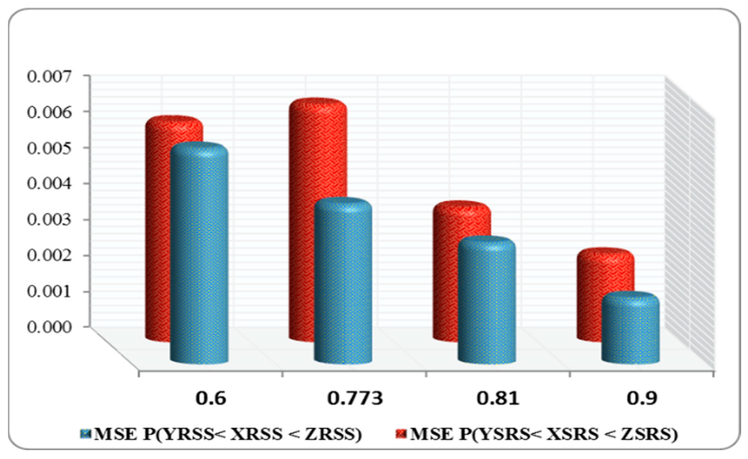
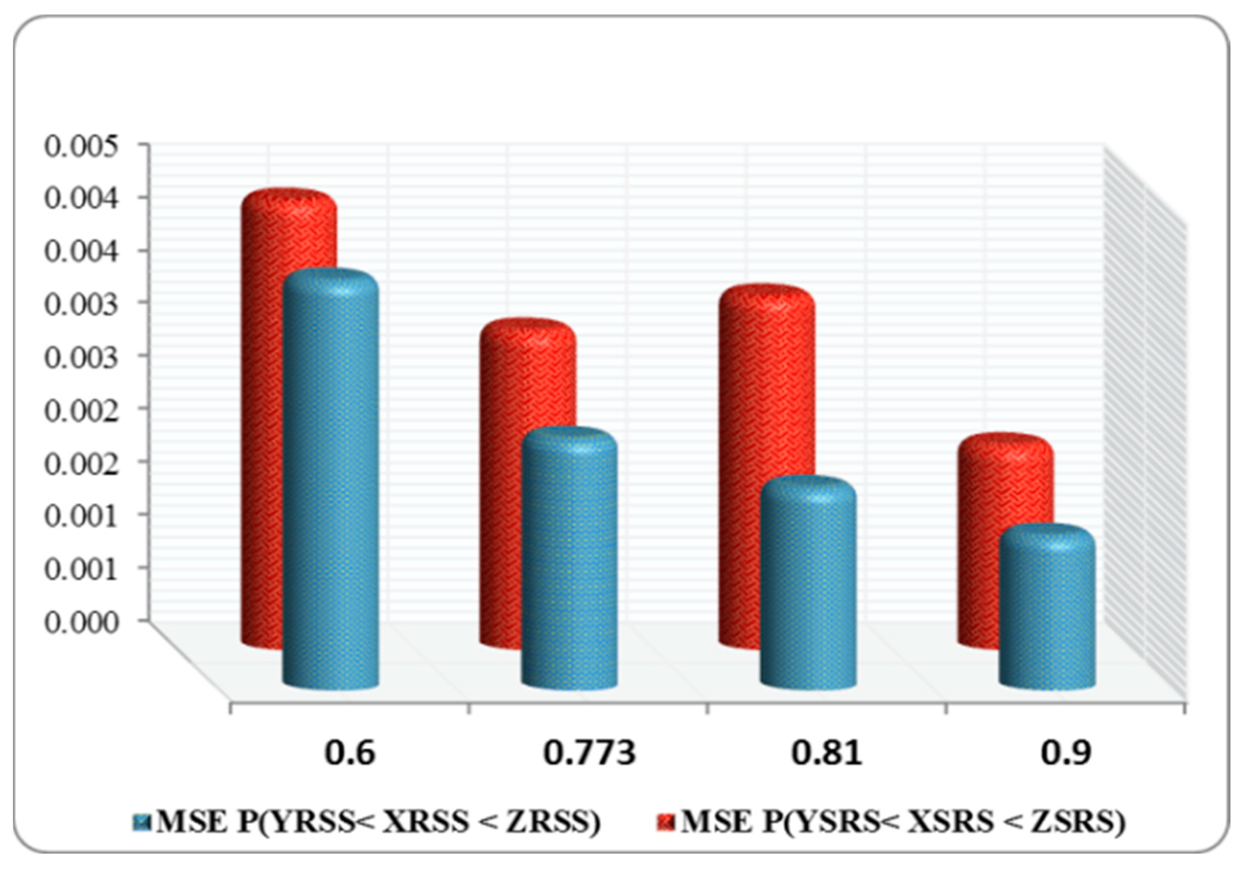
The values of the AB, SE, MSE, and RE are summarized in Table 1, Table 2, Table 3, Table 4, Table 5, Table 6, Table 7 and Table 8. From the numerical outcomes given in Table 1, Table 2, Table 3, Table 4, Table 5, Table 6, Table 7 and Table 8 and Figure 3, Figure 4, Figure 5 and Figure 6, we can conclude the following:

Table 1. Measurements of ${\widehat{ℝ}}_1$ and ${\widehat{ℝ}}_2$ for sampling schemes at $ℝ$ = 0.9 and d = 5.

$({\mathit{n}}_2^{*},{\mathit{n}}_1^{*},{\mathit{n}}_3^{*})$	$\mathit{P}\left({\mathit{Y}}_{\mathit{S}\mathit{R}\mathit{S}}<{\mathit{X}}_{\mathit{S}\mathit{R}\mathit{S}}<{\mathit{Z}}_{\mathit{S}\mathit{R}\mathit{S}}\right)$				$({\mathit{n}}_2,{\mathit{n}}_1,{\mathit{n}}_3)$	$\mathit{P}\left({\mathit{Y}}_{\mathit{R}\mathit{S}\mathit{S}}<{\mathit{X}}_{\mathit{R}\mathit{S}\mathit{S}}<{\mathit{Z}}_{\mathit{R}\mathit{S}\mathit{S}}\right)$				$\mathit{R}{\mathit{E}}_1(\widehat{\mathbf{ℝ}})$
	AB	SE	MSE	${\widehat{\mathbf{ℝ}}}_1$		AB	SE	MSE	${\widehat{\mathbf{ℝ}}}_2$
(10,10,10)	0.0110	0.0483	0.00245	0.88881	(2,2,2)	0.0100	0.04182	0.00185	0.88983	1.32
(20,20,20)	0.0081	0.0221	0.00055	0.89171	(4,4,4)	0.0145	0.02617	0.00089	0.88535	0.62
(30,30,30)	0.0053	0.0209	0.00047	0.89458	(6,6,6)	0.0152	0.01823	0.00056	0.88464	0.84
(20,10,20)	0.0059	0.0292	0.00089	0.89384	(4,2,4)	0.0134	0.03683	0.00154	0.88645	0.58
(30,10,30)	0.0479	0.0482	0.00462	0.85184	(6,2,6)	0.0158	0.02462	0.00085	0.88406	5.44
(10,20,10)	0.0072	0.0379	0.00149	0.89268	(2,4,2)	0.0137	0.03694	0.00155	0.88616	0.96
(10,30,10)	0.0146	0.0414	0.00193	0.88523	(2,6,2)	0.0166	0.03438	0.00146	0.88323	1.32
(30,20,30)	0.00629	0.0244	0.00064	0.89354	(6,4,6)	0.01487	0.02035	0.00064	0.88496	1.00
(20,30,20)	0.00930	0.0231	0.00062	0.89053	(4,6,4)	0.01553	0.02396	0.00082	0.88430	0.76

Table 2. Measurements of ${\widehat{ℝ}}_3$ and ${\widehat{ℝ}}_4$ for sampling schemes at $ℝ$ = 0.9 and d = 5.

$({\mathit{n}}_2,{\mathit{n}}_1^{*},{\mathit{n}}_3)$	$\mathit{P}\left({\mathit{Y}}_{\mathit{R}\mathit{S}\mathit{S}}<{\mathit{X}}_{\mathit{S}\mathit{R}\mathit{S}}<{\mathit{Z}}_{\mathit{R}\mathit{S}\mathit{S}}\right)$				$({\mathit{n}}_2^{*},{\mathit{n}}_1,{\mathit{n}}_3^{*})$	$\mathit{P}\left({\mathit{Y}}_{\mathit{S}\mathit{R}\mathit{S}}<{\mathit{X}}_{\mathit{R}\mathit{S}\mathit{S}}<{\mathit{Z}}_{\mathit{S}\mathit{R}\mathit{S}}\right)$				$\mathit{R}{\mathit{E}}_2(\widehat{\mathbf{ℝ}})$
	AB	SE	MSE	${\widehat{\mathbf{ℝ}}}_3$		AB	SE	MSE	${\widehat{\mathbf{ℝ}}}_4$
(2,10,2)	0.0130	0.02510	0.00080	0.91283	(10,2,10)	0.00606	0.04109	0.00172	0.9059	0.47
(4,20,4)	0.0171	0.02240	0.00079	0.91692	(20,4,20)	0.00311	0.02765	0.00077	0.90294	1.03
(6,30,6)	0.0163	0.01694	0.00055	0.91612	(30,6,30)	0.00093	0.0218	0.00048	0.90077	1.15
(4,10,4)	0.0123	0.02535	0.00080	0.91217	(20,2,20)	0.0034	0.03279	0.00109	0.90323	0.73
(6,10,6)	0.0101	0.02057	0.00053	0.90997	(30,2,30)	0.00177	0.02753	0.00076	0.9016	0.70
(2,20,2)	0.0107	0.03324	0.00122	0.91056	(10,4,10)	0.00305	0.03687	0.00137	0.90288	0.89
(2,30,2)	0.0110	0.02984	0.00101	0.91085	(10,6,10)	0.00036	0.0329	0.00108	0.90019	0.94
(6,20,6)	0.0146	0.01709	0.00051	0.91445	(30,4,30)	0.00152	0.02391	0.00057	0.90136	0.89
(4,30,4)	0.0175	0.02037	0.00072	0.91736	(20,6,20)	0.00096	0.02501	0.00063	0.9008	1.14

Table 3. Measurements of ${\widehat{ℝ}}_1$ and ${\widehat{ℝ}}_2$ for different sampling schemes at $ℝ$ = 0.81 and d = 5.

$({\mathit{n}}_2^{*},{\mathit{n}}_1^{*},{\mathit{n}}_3^{*})$	$\mathit{P}\left({\mathit{Y}}_{\mathit{S}\mathit{R}\mathit{S}}<{\mathit{X}}_{\mathit{S}\mathit{R}\mathit{S}}<{\mathit{Z}}_{\mathit{S}\mathit{R}\mathit{S}}\right)$				$({\mathit{n}}_2,{\mathit{n}}_1,{\mathit{n}}_3)$	$\mathit{P}\left({\mathit{Y}}_{\mathit{R}\mathit{S}\mathit{S}}<{\mathit{X}}_{\mathit{R}\mathit{S}\mathit{S}}<{\mathit{Z}}_{\mathit{R}\mathit{S}\mathit{S}}\right)$				$\mathit{R}{\mathit{E}}_1(\widehat{\mathbf{ℝ}})$
	AB	SE	MSE	${\widehat{\mathbf{ℝ}}}_1$		AB	SE	MSE	${\widehat{\mathbf{ℝ}}}_2$
(10,10,10)	0.0272	0.05488	0.00375	0.78287	(2,2,2)	0.00787	0.05771	0.00339	0.81796	1.11
(20,20,20)	0.0009	0.03774	0.00142	0.81098	(4,4,4)	0.00390	0.03500	0.00124	0.81398	1.15
(30,30,30)	0.0002	0.03631	0.00132	0.80996	(6,6,6)	0.00330	0.02498	0.00064	0.81338	2.06
(30,10,30)	0.0034	0.04114	0.00170	0.80670	(6,2,6)	0.00128	0.02967	0.00088	0.81136	1.93
(10,20,10)	0.0319	0.08350	0.00799	0.77814	(2,4,2)	0.00599	0.04876	0.00241	0.81607	3.32
(10,30,10)	0.0053	0.05750	0.00333	0.80477	(2,6,2)	0.00396	0.04348	0.00191	0.81404	1.74
(30,20,30)	0.0023	0.03853	0.00149	0.80774	(6,4,6)	0.00407	0.02659	0.00072	0.81415	2.07
(20,30,20)	0.0006	0.04367	0.00191	0.81069	(4,6,4)	0.00397	0.03223	0.00105	0.81405	1.82

Table 4. Measurements of ${\widehat{ℝ}}_3$ and ${\widehat{ℝ}}_4$ for different sampling schemes at $ℝ$ = 0.81 and d = 5.

$({\mathit{n}}_2,{\mathit{n}}_1^{*},{\mathit{n}}_3)$	$\mathit{P}\left({\mathit{Y}}_{\mathit{R}\mathit{S}\mathit{S}}<{\mathit{X}}_{\mathit{S}\mathit{R}\mathit{S}}<{\mathit{Z}}_{\mathit{R}\mathit{S}\mathit{S}}\right)$				$({\mathit{n}}_2^{*},{\mathit{n}}_1,{\mathit{n}}_3^{*})$	$\mathit{P}\left({\mathit{Y}}_{\mathit{S}\mathit{R}\mathit{S}}<{\mathit{X}}_{\mathit{R}\mathit{S}\mathit{S}}<{\mathit{Z}}_{\mathit{S}\mathit{R}\mathit{S}}\right)$				$\mathit{R}{\mathit{E}}_2(\widehat{\mathbf{ℝ}})$
	AB	SE	MSE	${\widehat{\mathbf{ℝ}}}_3$		AB	SE	MSE	${\widehat{\mathbf{ℝ}}}_4$
(2,10,2)	0.0165	0.05901	0.00375	0.82654	(10,2,10)	0.00072	0.06388	0.00408	0.80936	0.92
(4,20,4)	0.0223	0.03439	0.00168	0.83239	(20,4,20)	0.00559	0.04316	0.00189	0.80449	0.89
(6,30,6)	0.0188	0.02362	0.00091	0.79128	(30,6,30)	0.00801	0.03569	0.00134	0.80207	0.68
(4,10,4)	0.0178	0.03867	0.00181	0.82784	(20,2,20)	0.00750	0.04821	0.00238	0.80258	0.76
(6,10,6)	0.0148	0.03717	0.00160	0.82489	(30,2,30)	0.00670	0.04119	0.00174	0.80338	0.92
(2,20,2)	0.0159	0.05065	0.00282	0.82602	(10,4,10)	0.00897	0.05586	0.00320	0.80112	0.88
(2,30,2)	0.0168	0.04575	0.00238	0.82688	(10,6,10)	0.01359	0.05303	0.00300	0.79649	0.79
(6,20,6)	0.0228	0.02829	0.00132	0.83286	(30,4,30)	0.00733	0.03837	0.00153	0.80275	0.86
(4,30,4)	0.0242	0.03200	0.00161	0.83426	(20,6,20)	0.00761	0.04006	0.00166	0.80247	0.97

Table 5. Measurements of ${\widehat{ℝ}}_1$ and ${\widehat{ℝ}}_2$ for sampling schemes at $ℝ$ = 0.773 and d = 5.

$({\mathit{n}}_2^{*},{\mathit{n}}_1^{*},{\mathit{n}}_3^{*})$	$\mathit{P}\left({\mathit{Y}}_{\mathit{S}\mathit{R}\mathit{S}}<{\mathit{X}}_{\mathit{S}\mathit{R}\mathit{S}}<{\mathit{Z}}_{\mathit{S}\mathit{R}\mathit{S}}\right)$				$({\mathit{n}}_2,{\mathit{n}}_1,{\mathit{n}}_3)$	$\mathit{P}\left({\mathit{Y}}_{\mathit{R}\mathit{S}\mathit{S}}<{\mathit{X}}_{\mathit{R}\mathit{S}\mathit{S}}<{\mathit{Z}}_{\mathit{R}\mathit{S}\mathit{S}}\right)$				$\mathit{R}{\mathit{E}}_1(\widehat{\mathbf{ℝ}})$
	AB	SE	MSE	${\widehat{\mathbf{ℝ}}}_1$		AB	SE	MSE	${\widehat{\mathbf{ℝ}}}_2$
(10,10,10)	0.0018	0.08127	0.00661	0.77079	(2,2,2)	0.00416	0.06664	0.00446	0.77677	1.48
(20,20,20)	0.0073	0.05741	0.00335	0.76537	(4,4,4)	0.00292	0.03620	0.00132	0.77553	2.54
(30,30,30)	0.0103	0.05534	0.00317	0.76229	(6,6,6)	0.00318	0.02536	0.00065	0.77579	4.88
(20,10,20)	0.0273	0.05340	0.00359	0.79986	(4,2,4)	0.00075	0.03528	0.00125	0.77335	2.87
(30,10,30)	0.0023	0.06634	0.00441	0.77028	(6,2,6)	0.00075	0.03528	0.00125	0.77335	3.53
(10,20,10)	0.0389	0.05865	0.00496	0.73363	(2,4,2)	0.00140	0.05372	0.00289	0.77401	1.72
(10,30,10)	0.0195	0.05127	0.00301	0.7921	(2,6,2)	0.00058	0.04866	0.00237	0.77319	1.27
(30,20,30)	0.0089	0.02982	0.00097	0.78154	(6,4,6)	0.00294	0.02816	0.00080	0.77555	1.21
(20,30,20)	0.0316	0.04057	0.00264	0.74104	(4,6,4)	0.00304	0.03455	0.00120	0.77565	2.20

Table 6. Measurements of ${\widehat{ℝ}}_3$ and ${\widehat{ℝ}}_4$ for sampling schemes at $ℝ$ = 0.773 and d = 5.

$({\mathit{n}}_2,{\mathit{n}}_1^{*},{\mathit{n}}_3)$	$\mathit{P}\left({\mathit{Y}}_{\mathit{R}\mathit{S}\mathit{S}}<{\mathit{X}}_{\mathit{S}\mathit{R}\mathit{S}}<{\mathit{Z}}_{\mathit{R}\mathit{S}\mathit{S}}\right)$				$({\mathit{n}}_2^{*},{\mathit{n}}_1,{\mathit{n}}_3^{*})$	$\mathit{P}\left({\mathit{Y}}_{\mathit{S}\mathit{R}\mathit{S}}<{\mathit{X}}_{\mathit{R}\mathit{S}\mathit{S}}<{\mathit{Z}}_{\mathit{S}\mathit{R}\mathit{S}}\right)$				$\mathit{R}{\mathit{E}}_2(\widehat{\mathbf{ℝ}})$
	AB	SE	MSE	${\widehat{\mathbf{ℝ}}}_3$		AB	SE	MSE	${\widehat{\mathbf{ℝ}}}_4$
(2,10,2)	0.0301	0.05675	0.00413	0.80279	(10,2,10)	0.00351	0.07160	0.00514	0.77612	0.80
(4,20,4)	0.0554	0.03235	0.00412	0.82803	(20,4,20)	0.00396	0.04729	0.00225	0.77657	1.83
(6,30,6)	0.0691	0.02140	0.00524	0.84175	(30,6,30)	0.00009	0.03847	0.00148	0.77270	3.54
(4,10,4)	0.0523	0.03488	0.00395	0.82487	(20,2,20)	0.00359	0.05613	0.00316	0.77619	1.25
(6,10,6)	0.0645	0.02438	0.00475	0.83709	(30,2,30)	0.00214	0.04492	0.00202	0.77475	2.35
(2,20,2)	0.0306	0.05382	0.00383	0.80317	(10,4,10)	0.00159	0.06253	0.00391	0.77420	0.98
(2,30,2)	0.0299	0.05120	0.00352	0.80256	(10,6,10)	0.00106	0.05941	0.00353	0.77155	1.00
(6,20,6)	0.0682	0.02319	0.00519	0.84079	(30,4,30)	0.00232	0.04096	0.00168	0.77493	3.09
(4,30,4)	0.0566	0.02947	0.00407	0.82917	(20,6,20)	0.00181	0.04488	0.00202	0.77080	2.01

Table 7. Measurements of ${\widehat{ℝ}}_1$ and ${\widehat{ℝ}}_2$ for sampling schemes at $ℝ$ = 0.694 and d = 5.

$({\mathit{n}}_2^{*},{\mathit{n}}_1^{*},{\mathit{n}}_3^{*})$	$\mathit{P}\left({\mathit{Y}}_{\mathit{S}\mathit{R}\mathit{S}}<{\mathit{X}}_{\mathit{S}\mathit{R}\mathit{S}}<{\mathit{Z}}_{\mathit{S}\mathit{R}\mathit{S}}\right)$				$({\mathit{n}}_2,{\mathit{n}}_1,{\mathit{n}}_3)$	$\mathit{P}\left({\mathit{Y}}_{\mathit{R}\mathit{S}\mathit{S}}<{\mathit{X}}_{\mathit{R}\mathit{S}\mathit{S}}<{\mathit{Z}}_{\mathit{R}\mathit{S}\mathit{S}}\right)$				$\mathit{R}{\mathit{E}}_1(\widehat{\mathbf{ℝ}})$
	AB	SE	MSE	${\widehat{\mathbf{ℝ}}}_1$		AB	SE	MSE	${\widehat{\mathbf{ℝ}}}_2$
(10,10,10)	0.0340	0.07046	0.00612	0.66042	(2,2,2)	0.00962	0.07688	0.00600	0.70407	1.02
(20,20,20)	0.0303	0.04253	0.00273	0.72478	(4,4,4)	0.00520	0.04342	0.00191	0.69965	1.43
(30,30,30)	0.0021	0.03874	0.00151	0.69236	(6,6,6)	0.00376	0.02996	0.00091	0.69820	1.66
(20,10,20)	0.0334	0.04808	0.00343	0.66102	(4,2,4)	0.00251	0.05278	0.00279	0.69695	1.23
(30,10,30)	0.0569	0.03504	0.00447	0.75137	(6,2,6)	0.00440	0.04551	0.00209	0.69885	2.14
(10,20,10)	0.0529	0.07051	0.00777	0.64159	(2,4,2)	0.00376	0.06645	0.00443	0.69821	1.75
(10,30,10)	0.0047	0.06488	0.00423	0.68972	(2,6,2)	0.00139	0.06209	0.00386	0.69306	1.10
(30,20,30)	0.0234	0.03663	0.00189	0.71782	(6,4,6)	0.00516	0.03250	0.00108	0.69960	1.75
(20,30,20)	0.0334	0.04152	0.00284	0.72789	(4,6,4)	0.00143	0.04013	0.00161	0.69587	1.76

Table 8. Measurements of ${\widehat{ℝ}}_3$ and ${\widehat{ℝ}}_4$ for sampling schemes at $ℝ$= 0.694 and d = 5.

$({\mathit{n}}_2,{\mathit{n}}_1^{*},{\mathit{n}}_3)$	$\mathit{P}\left({\mathit{Y}}_{\mathit{R}\mathit{S}\mathit{S}}<{\mathit{X}}_{\mathit{S}\mathit{R}\mathit{S}}<{\mathit{Z}}_{\mathit{R}\mathit{S}\mathit{S}}\right)$				$({\mathit{n}}_2^{*},{\mathit{n}}_1,{\mathit{n}}_3^{*})$	$\mathit{P}\left({\mathit{Y}}_{\mathit{S}\mathit{R}\mathit{S}}<{\mathit{X}}_{\mathit{R}\mathit{S}\mathit{S}}<{\mathit{Z}}_{\mathit{S}\mathit{R}\mathit{S}}\right)$				$\mathit{R}{\mathit{E}}_2(\widehat{\mathbf{ℝ}})$
	AB	SE	MSE	${\widehat{\mathbf{ℝ}}}_3$		AB	SE	MSE	${\widehat{\mathbf{ℝ}}}_4$
(2,10,2)	0.0432	0.07127	0.00695	0.73766	(10,2,10)	0.00603	0.08770	0.00773	0.70048	0.90
(4,20,4)	0.0769	0.03659	0.00725	0.77135	(20,4,20)	0.00204	0.05571	0.00311	0.69649	2.33
(6,30,6)	0.0972	0.02294	0.00997	0.79161	(30,6,30)	0.00536	0.04429	0.00199	0.69981	5.01
(4,10,4)	0.0756	0.04008	0.00732	0.77003	(20,2,20)	0.00354	0.06535	0.00428	0.69798	1.71
(6,10,6)	0.0916	0.02664	0.00910	0.78602	(30,2,30)	0.00444	0.06053	0.00368	0.69889	2.47
(2,20,2)	0.0381	0.06836	0.00612	0.73250	(10,4,10)	0.00054	0.07763	0.00603	0.69499	1.01
(2,30,2)	0.0356	0.06448	0.00542	0.73002	(10,6,10)	0.00206	0.07335	0.00538	0.69238	1.01
(6,20,6)	0.0940	0.02531	0.00947	0.78842	(30,4,30)	0.00579	0.04813	0.00235	0.70023	4.03
(4,30,4)	0.0783	0.03428	0.00731	0.77274	(20,6,20)	0.00186	0.05225	0.00273	0.69630	2.68

Figure 3. MSE of ${\widehat{ℝ}}_1$ and ${\widehat{ℝ}}_2$ for $\left(n_2^{*},n_1^{*},n_3^{*}\right)=\left(10,10,10\right)$ at different values of $ℝ$.

Figure 4. MSE of ${\widehat{ℝ}}_1$ and ${\widehat{ℝ}}_2$ for $\left(n_2^{*},n_1^{*},n_3^{*}\right)=\left(10,30,10\right)$ at different values of $ℝ$.

Figure 5. MSE of ${\widehat{ℝ}}_3$ and ${\widehat{ℝ}}_4$ for $\left(n_2,n_1^{*},n_3\right)=\left(2,20,2\right)$ at different values of $ℝ$.

Figure 6. MSE of ${\widehat{ℝ}}_3$ and ${\widehat{ℝ}}_4$ for $\left(n_2,n_1^{*},n_3\right)=\left(4,20,4\right)$ at different values of $ℝ$.

▪

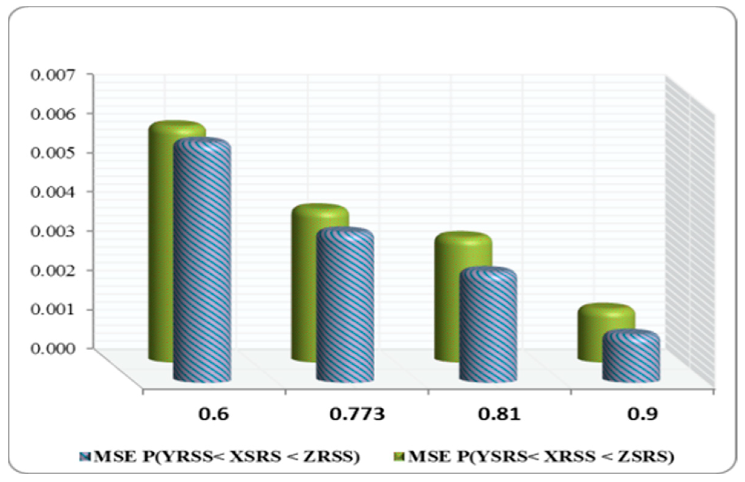
Table 3 and Table 5 indicate that, in all cases, where $ℝ$ = 0.81 and 0.773, the reliability estimates obtained using the RSS approach were more efficient than those obtained using the SRS scheme.

▪

At the true value $ℝ$ = 0.81, the MSEs of ${\widehat{ℝ}}_3=P\left(Y_{RSS}<X_{SRS}<Z_{RSS}\right)$ were more efficient than ${\widehat{ℝ}}_4=P\left(Y_{SRS}<X_{RSS}<Z_{SRS}\right)$ in all cases (see Table 4).

In most cases, as seen in Figure 3, Figure 4, Figure 5 and Figure 6, the MSEs of ${\widehat{ℝ}}_1,{\widehat{ℝ}}_2,{\widehat{ℝ}}_3$, and ${\widehat{ℝ}}_4$ decreased with an increased value of $ℝ$.

▪

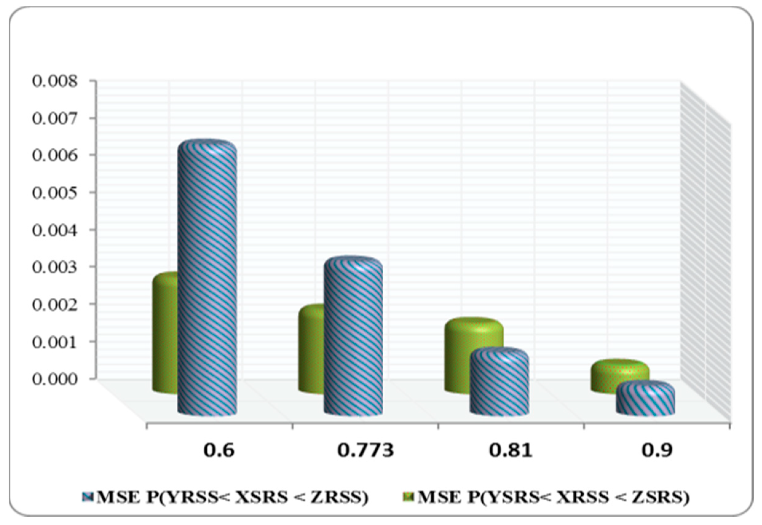
Table 7 shows that ${\widehat{ℝ}}_2$ is more efficient than ${\widehat{ℝ}}_1$ in all situations.

▪

In most instances, the ABs of SSR estimates in all schemes diminished as the true value of $ℝ$ rises (see Table 1, Table 2, Table 3, Table 4, Table 5, Table 6, Table 7 and Table 8).

▪

For all true values of $ℝ$ where $\left(n_2^{*},n_1^{*},n_3^{*}\right)=$(30,30,30), (30,20,30), (20,30,20), (10,30,10), and (10,20,10), the SEs of ${\widehat{ℝ}}_1$ based on the SRS, had larger values compared to ${\widehat{ℝ}}_2,$ via the RSS (see Table 1, Table 3, Table 5 and Table 7).

▪

The SEs of ${\widehat{ℝ}}_3$ had the lowest values when compared to ${\widehat{ℝ}}_4,$ for all true values of $ℝ$ and sample sizes (see Table 2, Table 4 and Table 6).

▪

The MSEs of ${\widehat{ℝ}}_3$ gave the lowest values comparable with ${\widehat{ℝ}}_4$ for all sample sizes at $ℝ$ = 0.694 except for $(n_2,n_1^{*},n_3$) = (2,10,2) (see Table 8).

▪

Table 6 clearly indicates that the MSEs of ${\widehat{ℝ}}_3$ are the lowest when compared with ${\widehat{ℝ}}_4$ for all sample sizes at $ℝ$ = 0.773 with the exception of $(n_2,n_1^{*},n_3$) = (2,10,2) and (2,20,2).

▪

For all sample sizes, at actual value $ℝ$ = 0.81, the MSEs of ${\widehat{ℝ}}_2$ and ${\widehat{ℝ}}_3$ had the minimum values compared with ${\widehat{ℝ}}_1$ and ${\widehat{ℝ}}_4,$ respectively (see Table 3 and Table 4).

▪

Except for in a few cases, the MSEs of ${\widehat{ℝ}}_2$ obtained the minimum values when compared to ${\widehat{ℝ}}_1$ for all the sample size values (see Table 1, Table 3, Table 5 and Table 7).

9. Data Analysis

In this section, three data sets were considered and are described in detail, to illustrate the usefulness of the proposed models. The first two data sets were originally documented in [36], and they show the strength measured in GPA for single carbon fibers of lengths of 10 mm ($Y$: Data I, n₂ = 63) and 20 mm ($X$: Data II, n₁ = 69), which fit the GIED model (see [17]). The Kolmogorov–Smirnov (K-S) distances were 0.086, and 0.041 for Data I and II, with 0.739 and 0.999 p-values, respectively. The fitted models based on these two data sets are provided in Figure 7.

Figure 7. Estimated PDF and CDF plots using Data I and II for the GIED.

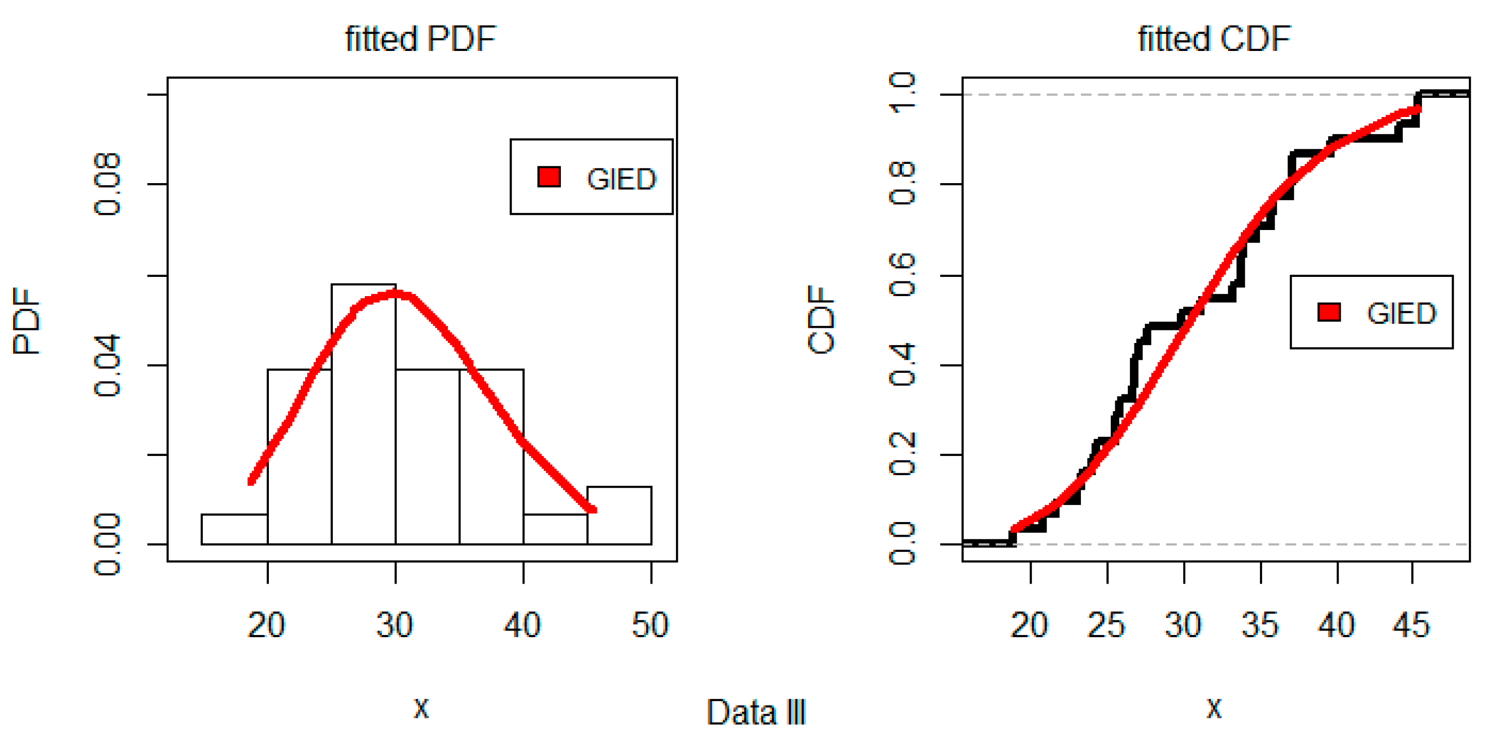
The set Data III ($Z$) was provided by Ed Fuller of the NICT Ceramics Division in December 1993. It contains n₃ = 31 polished window strength data. Ref. [37] described the use of this set to predict the lifetime of a glass airplane window. Here, we tested Data III against the fitted model using a KS test, where its distance was 0.138 and the corresponding p-value was 0.595. This shows that the GIED fits this data set rather well. Figure 8 shows the estimated PDF and CDF for the Data III. The GIED appeared to be an appropriate model for fitting these data based on this graph.

Figure 8. Estimated PDF and CDF plots using Data III for the GIED.

The RSS and SRS sampling procedures were used to examine real data sets based on the preceding theoretical conclusions. The RSS and SRS were produced using the R-package RSSampling and Data I, II, and III. The SSR estimates were calculated in the following cases:

(i)

SS models with common scale parameters

Assuming that the strength $X$~GIED$(\delta ,{\vartheta }_1),$ the stress $Y$~GIED$(\delta ,{\vartheta }_2)$, and stress $Z$~GIED$(\delta ,{\vartheta }_3)$, where $X$, $Y$ and $Z$ are independent random variables. The SSR estimates were calculated from the GIED for different values of set size under five cycles, using four distinct scenarios, as seen in Table 9.

Table 9. SSR estimates of the data sets based on different sampling designs.

(n2*, n1*, n3*)	${\widehat{\mathbf{ℝ}}}_1$	(n2, n1, n3)	${\widehat{\mathbf{ℝ}}}_2$	(n2, n1*, n3)	${\widehat{\mathbf{ℝ}}}_3$	(n2*, n1, n3*)	${\widehat{\mathbf{ℝ}}}_4$
(10,20,10)	0.262	(2,4,2)	0.497	(2,20,2)	0.331	(10,4,10)	0.195
(10,10,10)	0.258	(2,2,2)	0.503	(2,10,2)	0.204	(10,2,10)	0.125
(20,20,20)	0.172	(4,4,4)	0.396	(4,20,4)	0.268	(20,4,20)	0.154
(30,30,30)	0.168	(6,6,6)	NA*	(6,30,6)	NA*	(30,6,30)	0.148
(20,10,20)	0.173	(4,2,4)	0.349	(4,10,4)	0.244	(20,2,20)	0.192
(30,10,30)	0.166	(6,2,6)	NA*	(6,10,6)	NA*	(30,2,30)	0.17
(10,30,10)	0.263	(2,6,2)	0.469	(2,30,2)	0.351	(10,6,10)	0.194
(30,20,30)	0.168	(6,4,6)	NA*	(6,20,6)	NA*	(30,4,30)	0.169
(20,30,20)	0.171	(4,6,4)	0.421	(4,30,4)	0.279	(20,6,20)	0.147

Note that, NA* in Table 9 means that there were no estimates available for some cases, since we needed at least 36 observations to obtain an RSS of size 6, while the strength random variable X only had 31 observations.

(ii)

The SS models with dissimilar scale parameters

Suppose that $X$~GIED$({\delta }_1,{\vartheta }_1),$ Y~GIED$({\delta }_2,{\vartheta }_2),$, and $Z$~GIED$({\delta }_3,{\vartheta }_3),$ the ML estimates of the model parameters and the SSR estimates were calculated under different RSS and SRS using the four proposed sample cases. In addition, the Fisher information matrices as well as their corresponding SEs are displayed between parentheses using Data I, II, and III. Table 10 presents the parameter estimates, SSR estimates, and SEs for the different RSS and SRS.

Table 10. Parameter and SSR estimates of the data sets and their corresponding SE based on the different sampling designs.

${\mathbf{ℝ}}_1=\hspace{0.17em}\mathit{P}[{\mathit{Y}}_{\mathit{S}\mathit{R}\mathit{S}}<{\mathit{X}}_{\mathit{S}\mathit{R}\mathit{S}}<{\mathit{Z}}_{\mathit{S}\mathit{R}\mathit{S}}]$
(n2*, n1*, n3*)	${\widehat{ℝ}}_1$	X		Y		Z
		${\vartheta }_1$	${\delta }_1$	${\vartheta }_2$	${\delta }_2$	${\vartheta }_3$	${\delta }_3$
(10,20,10)	0.044	136.74	12.203	464.533	18.346	859.909	17.504
		(30.576)	(0.575)	(146.898)	(0.993)	(328.811)	(1.169)
(10,10,10)	0.028	86.513	10.075	464.44	18.346	905.014	17.618
		(27.358)	(0.738)	(146.869)	(0.993)	(346.737)	(1.173)
(20,20,20)	0.591	136.721	12.202	275.022	17.868	13.064	6.89
		(30.572)	(0.575)	(61.497)	(0.554)	(3.516)	(0.594)
(30,30,30)	0.418	184.861	13.43	169.623	16.464	17.202	7.502
		(33.751)	(0.488)	(30.969)	(0.364)	(3.985)	(0.493)
(20,10,20)	0.446	86.459	10.073	128.725	15.401	19.757	7.757
		(27.341)	(0.738)	(28.784)	(0.543)	(5.439)	(0.603)
(30,10,30)	0.426	86.459	10.073	84.472	14.156	8.842	6.198
		(27.341)	(0.738)	(15.422)	(0.351)	(1.907)	(0.487)
(10,30,10)	0.05	185.822	13.444	464.625	18.347	910.172	17.631
		(33.926)	(0.488)	(146.927)	(0.993)	(348.789)	(1.173)
(30,20,30)	0.58	136.721	12.202	250.948	17.792	11.494	6.783
		(30.572)	(0.575)	(45.817)	(0.371)	(2.544)	(0.497)
(20,30,20)	0.363	185.171	13.435	124.577	15.334	12.089	6.616
		(33.808)	(0.488)	(27.856)	(0.549)	(3.257)	(0.578)
${\mathbf{ℝ}}_{\mathbf{2}}\mathbf{=}\hspace{0.17em}\mathit{P}\mathbf{[}{\mathit{Y}}_{\mathit{R}\mathit{S}\mathit{S}}\mathbf{<}{\mathit{X}}_{\mathit{R}\mathit{S}\mathit{S}}\mathbf{<}{\mathit{Z}}_{\mathit{R}\mathit{S}\mathit{S}}\mathbf{]}$
(n*, n1, n3)	${\widehat{ℝ}}_{}{}_2$	X		Y		Z
		${\vartheta }_1$	${\delta }_1$	${\vartheta }_2$	${\delta }_2$	${\vartheta }_3$	${\delta }_3$
(2,4,2)	0.051	0.065	0.002	6.458	6.524	1.022	16.104
		(0.012)	(0.002)	(1.686)	(0.588)	(0.268)	(4.134)
(2,2,2)	0.0002	0.04	0.002	99.633	14.243	112.209	153.077
		(0.018)	(0.006)	(26.446)	(0.683)	(30.166)	(8.944)
(4,4,4)	0.058	0.063	0.001	2.57	4.203	0.767	12.973
		(0.012)	(0.002)	(0.368)	(0.142)	(0.111)	(2.154)
(4,2,4)	0.0006	0.04	0.002	12.862	8.749	180.806	170.194
		(0.018)	(0.006)	(1.851)	(0.193)	(27.027)	(4.89)
(2,6,2)	0.001	0.242	0.275	99.633	14.243	112.209	153.077
		(0.028)	(0.074)	(26.446)	(0.683)	(30.166)	(8.944)
(4,6,4)	0.0008	0.242	0.275	12.862	8.749	180.806	170.194
		(0.028)	(0.074)	(1.851)	(0.193)	(27.027)	(4.89)
${\mathbf{ℝ}}_{\mathbf{3}}\mathbf{=}\hspace{0.17em}\mathit{P}\mathbf{[}{\mathit{Y}}_{\mathit{R}\mathit{S}\mathit{S}}\mathbf{<}{\mathit{X}}_{\mathit{S}\mathit{R}\mathit{S}}\mathbf{<}{\mathit{Z}}_{\mathit{R}\mathit{S}\mathit{S}}\mathbf{]}$
(n2, n1*, n3)	${\widehat{ℝ}}_3$	X		Y		Z
		${\vartheta }_1$	${\delta }_1$	${\vartheta }_2$	${\delta }_2$	${\vartheta }_3$	${\delta }_3$
(2,10,2)	0.145	86.459	10.073	99.633	14.243	112.209	153.077
		(27.341)	(0.738)	(26.446)	(0.683)	(30.166)	(8.944)
(4,20,4)	0.016	100.123	12.17	12.862	8.749	180.806	170.194
		(22.388)	(0.617)	(1.851)	(0.193)	(27.027)	(4.89)
(4,10,4)	0.017	227.816	14.457	12.862	8.749	180.806	170.194
		(72.042)	(0.888)	(1.851)	(0.193)	(27.027)	(4.89)
(2,20,2)	0.151	100.123	12.17	99.633	14.243	112.209	153.077
		(22.388)	(0.617)	(26.446)	(0.683)	(30.166)	(8.944)
(2,30,2)	0.158	151.844	13.712	99.633	14.243	112.209	153.077
		(27.723)	(0.521)	(26.446)	(0.683)	(30.166)	(8.944)
(4,30,4)	0.017	151.844	13.712	12.862	8.749	180.806	170.194
		(27.723)	(0.521)	(1.851)	(0.193)	(27.027)	(4.89)
${\mathbf{ℝ}}_{\mathbf{4}}\mathbf{=}\hspace{0.17em}\mathit{P}[{\mathit{Y}}_{\mathit{S}\mathit{R}\mathit{S}}\mathbf{<}{\mathit{X}}_{\mathit{R}\mathit{S}\mathit{S}}\mathbf{<}{\mathit{Z}}_{\mathit{S}\mathit{R}\mathit{S}}\mathbf{]}$
(n2*, n1, n3*)	${\widehat{ℝ}}_4$	X		Y		Z
		${\vartheta }_1$	${\delta }_1$	${\vartheta }_2$	${\delta }_2$	${\vartheta }_3$	${\delta }_3$
(10,2,10)	0.0057	0.04	0.002	3.487	5.14	3.446	5.028
		(0.018)	(0.006)	(1.103)	(0.92)	(1.124)	(0.963)
(20,4,20)	0.018	0.19	0.205	4.999	6.281	4.935	6.064
		(0.035)	(0.097)	(1.118)	(0.527)	(1.177)	(0.742)
(20,2,20)	0.012	0.081	0.068	3.563	5.468	3.39	5.229
		(0.036)	(0.108)	(0.797)	(0.513)	(0.795)	(0.723)
(30,2,30)	0.009	0.084	0.079	4.54	6.168	4.313	5.892
		(0.038)	(0.121)	(0.829)	(0.363)	(0.833)	(0.613)
(10,4,10)	0.016	0.201	0.241	5.891	6.323	5.837	6.152
		(0.037)	(0.108)	(1.863)	(0.949)	(1.93)	(0.986)
(30,4,30)	0.0173	0.1832	0.1892	5.1301	6.4686	5.0659	6.2556
		(0.0338)	(0.0926)	(0.9366)	(0.3654)	(0.9858)	(0.6193)
(10,6,10)	0.031	0.274	0.361	4.31	5.607	4.114	5.399
		(0.032)	(0.088)	(1.363)	(0.933)	(1.347)	(0.972)
(20,6,20)	0.059	0.254	0.305	10.14	8.064	2.992	4.96
		(0.03)	(0.079)	(2.267)	(0.54)	(0.698)	(0.717)
(30,6,30)	0.0001	0.242	0.2746	450.6258	19.8243	1167.133	17.9341
		(0.0283)	(0.0738)	(82.2726)	(0.3843)	(249.2422)	(0.6769)

(iii)

Count Frequency of Data

Here, we calculate the empirical estimates of the probabilities P(Y < X < Z) from the equal samples X, Y, and Z, using different sampling designs from Data I, II, and III. These probabilities were obtained as count numbers by checking whether the samples from X, Y, and Z satisfied Y < X < Z. These calculations are provided in Table 11.

Table 11. Empirical probabilities of (Y < X < Z) using different sampling designs.

(n2*, n1*, n3*)	${\widehat{\mathbf{ℝ}}}_1$	(n2,n1,n3)	${\widehat{\mathbf{ℝ}}}_2$	(n2, n1*, n3)	${\widehat{\mathbf{ℝ}}}_3$	(n2*, n1, n3*)	${\widehat{\mathbf{ℝ}}}_4$
(10,10,10)	0.1	(2,2,2)	0	(2,10,2)	0.1	(10,2,10)	0.5
(20,20,20)	0.2	(4,4,4)	0.05	(4,20,4)	0.2	(20,4,20)	0.3
(30,30,30)	0.1667	(6,6,6)	NA*	(6,30,6)	NA*	(30,6,30)	0.2667

10. Conclusions

We considered estimating an SSR, say $ℝ=\hspace{0.17em}P[Y<X<Z],$ when the strength X is accompanied by two stresses, Y and Z, that are independent but not identically distributed random variables from the GIED. The SSR estimators were considered based on four scenarios for the situation of SRS and RSS. The SSR estimators were constructed when the strength data were acquired from the RSS, while the stress data were taken from the SRS, and conversely. In addition, the SSR estimators were produced when the strength and stress data were accessible from the RSS/SRS. Finally, a simulation procedure was employed to compare the results of the various estimators. Three data sets were used to provide a real-world example that produced the following findings. In general, we concluded that the SSR estimators were more efficient when the strength random variable X was based on RSS, rather than on the SRS scheme, no matter what the stresses were. It is hoped that our research will be valuable to researchers working with the data used in the present study.