Abstract
Traditional fault tree analysis is an effective tool used to evaluate system risk if the required data are sufficient. Unfortunately, the operation and maintenance data of some complex systems are difficult to obtain due to economic or technical reasons. The solution is to invite experts to evaluate some critical aspect of the performance of the system. In this study, the belief degrees of the occurrence of basic events evaluated by experts are measured by an uncertain measure. Then, a system risk assessment method based on an uncertain fault tree is proposed, based on which two general optimization models are established. Furthermore, the genetic algorithm (GA) and the nondominated sorting genetic algorithm II (NSGA-II) are applied to solve the two optimization models, separately. In addition, the proposed risk assessment method is applied for the leakage risk evaluation of a subsea production system, and the two general optimization models are used to optimize the leakage risk and maintenance cost of the subsea production system. The optimization results provide a theoretical basis for practitioners to guarantee the safety of subsea production system.
1. Introduction
Optimization between risk and cost is an important topic in the field of industrial and systems engineering. In past decades, researchers have paid attention to risk assessment and optimization methods for complex systems based on probability theory, such as Faddoul et al. [1], Hong et al. [2], Liu et al. [3], Ma et al. [4] and Yousefi et al. [5]. However, to take probability theory as a mathematical basis for risk evaluation and optimization, three basic premises need to be met at the same time: events need to be clearly defined; there are a large number of samples; there is probability repeatability between samples. and In the field of engineering, it is difficult to obtain sufficient data. Therefore, experts are invited to evaluate the technical condition of systems, which are often described with ambiguous language. In 1965, Zadeh [6] proposed the concept of fuzzy set to deal with imprecise and subjective information. After that, researchers began to deal with various optimization problems in fuzzy environments, such as Mortazavi [7], Sayyaadi and Baghsheikhi [8], Yang et al. [9], Zhou et al. [10], and so on. Unfortunately, Liu [11] showed that fuzzy theory is unsuitable for modeling belief degree via a counter example of the strength of a bridge. A similar situation exists in the field of system risk evaluation. For example, system risk is evaluated by experts as approximately 0.0. If the system risk is regarded as a triangular fuzzy variable (0.005, 0.01, 0.015), it can be concluded that the possibility of the system risk is exactly 0.01 is 1 and the possibility of the system risk is not 0.01 is 1 based on the possibility measure. It is usually thought that the possibility of the system risk is exactly 0.01 is 0. In addition, the system risk is exactly 0.01 and the system risk is not 0.01 have the same possibility measure. This contradictory conclusion also shows that the belief degree of experts is unsuitable for modeling by the possibility measure because it does not have a duality property.
In order to measure belief degree, uncertainty theory was founded by Liu [12] and refined by Liu [13] based on normality, duality, subadditivity, and product measure axioms. In recent years, uncertainty theory has been widely used in various fields, such as reliability analysis [14], inference controller [15], risk assessment [16], and statistics [17]. In terms of optimization problems, uncertainty theory is still an effective mathematical modeling tool. For instance, Ke and Yao [18] regarded the units as uncertain variables and proposed a block replacement strategy in uncertain environments. Liu et al. [19] gave the upper and lower bounds of insurance premiums with uncertain random losses and established a mathematical model of an optimal insurance problem. Zhang and Peng [20] solved the uncertain optimal assignment problem by giving the uncertainty distribution of the optimal assignment profit. Li et al. [21] regarded the return rate of risky assets as an uncertain variable and established an uncertain model for portfolio optimization. Li et al. [22] provided a new reliability metric that encompassed two types of task time uncertainties and developed a multiple objective to maximize the reliability and efficiency of assembly lines. Wen et al. [23] presented the minimal expected backorder model and the minimal backorder rate model with the constraints of costs and supply availability based on an uncertain measure. Li et al. [24] derived some useful theorems related to the optimal solutions by modeling the uncertain task time. Guo et al. [25] established a multiechelon multi-indenture optimization LORA model that took the best cost-effectiveness ratio as the criterion.
GA and NSGA-II, as well-known evolutionary algorithms for solving optimization problems, have been successfully applied to different real-world applications, including reliability optimization.
Andrews and Bartlett [26] used GA for the single objective optimization of a firewater deluge system on an offshore platform, in which the system was presented with the structure of a fault tree. Pattison and Andrews [27] described a design optimization scheme for systems that require a high likelihood of functioning on demand by using GA. Cui et al. [28] proposed a novel reliability design and optimization method of planetary gears using the GA, based on the Kriging model. Ardakan and Rezvan [29] considered the multiobjective optimization of the reliability–redundancy allocation problem with a cold-standby strategy using NSGA-II. Bhattacharyya and Cheliyan [30] solved a subsea production system optimization problem by using GA and NSGA-II, in which the risk was evaluated with fault tree analysis. Due to the advantages of GA and NSGA-II, we continued to use the above two algorithms to solve optimization models.
Subsea production systems are mainly composed of Xmas trees, manifolds, jumper tubes, umbilical cables, pipelines, etc. [31]. With the increase in service time of subsea production systems, more and more safety problems have emerged, especially leakage. The leakage of subsea production systems results in serious environment pollution and significant economic losses. Therefore, it is essential to ensure the safety of subsea production systems. Additionally, the total maintenance cost is expected as low as possible. Bhattacharyya and Cheliyan [30] paid attention to such problems and optimized the cost and reliability of a subsea production system on the basis of a traditional fault tree. Unfortunately, it is difficult to obtain sufficient data to evaluate the risk of subsea production systems. In this situation, experts must evaluate the key performance indicators of a subsea production system. Then, Cheliyan and Bhattacharyya [32] assessed the leakage risk of a subsea production system based on a fuzzy fault tree, in which the epistemic uncertainty was modeled with fuzzy set theory. Because the possibility measure has no duality property, a self-dual measure is absolutely needed in both theory and practice.
The major contributions of this study are as follows: A risk assessment method for complex systems with insufficient data is proposed based on uncertain fault tree analysis; two general optimization models are established for complex systems with insufficient data, and the GA and NSGA-II are applied to solve the two optimization models, separately. Leakage risk is evaluated; two optimization models of the leakage risk and maintenance cost are established for a subsea production system. Then, the optimization results are discussed.
The remainder of this paper is organized as follows Section 2 proposes a risk assessment method for systems with insufficient data. Section 3 establishes two general optimization models based on uncertain fault tree and describes the algorithms for solving the two optimization models. Section 4 outlines a leakage risk evaluation for a subsea production system, establishes the optimization models of maintenance cost and leakage risk for the subsea production system, and we discuss the optimization results. In addition, the steps of GA and NSGA-II are provided in Appendix A.
2. Risk Assessment Method Based on Uncertain Fault Tree
A fault tree is called an uncertain fault tree if the occurrences of the input events are evaluated by the uncertain measure proposed by Liu [12]. The system risk is the belief degree of the occurrence of the top event; for the operation rules, refer to Liu [33].
Theorem 1.
If are independent input events, the belief degree of the occurrence of output event Λ is
Proof.
If independent input events are connected by an “AND” gate, the belief degree of the occurrence of the output event can be derived by
If independent input events are connected by an “OR” gate, the belief degree of the occurrence of the output event can be derived by
The proof is completed. □
Example 1.
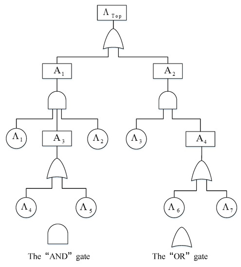

The fault tree shown in Figure 1 describes the system risk. , denote independent basic events, , denote the intermediate events, and denotes the top event in the fault tree. Table 1 lists the belief degrees of the occurrence of the basic events.

Figure 1.
A fault tree structure.

Table 1.
The belief degrees of the occurrence of basic events.
As shown in Figure 1, the top event can be expressed as
Then, the belief degree of occurrence of the top event can be determined, i.e., the risk of the top event , namely,
If the belief degree is replaced by probability in Example 1, then the risk of the top event can be calculated with the probability method, namely,
It can be seen that and are different, which implies when the data are sufficient, traditional fault tree analysis is applied to evaluate the probability of the occurrence of the top event; when the data are insufficient, uncertain fault tree analysis is used to evaluate the belief degree of the occurrence of the top event.
By comparison of and in Example 1, it can be seen that is larger than . However, this does not mean that is always larger than . For example, if and change to , then and Therefore, we cannot simply compare the values of and without knowing the fault tree structure and the belief degrees and probabilities of the occurrence of all basic events.
3. General Optimization Models Based on Uncertain Fault Tree
In this section, an uncertain fault tree is used to evaluate system risk. Then, a single-objective optimization model and a multiobjective optimization model based on uncertain fault tree are separately established.
Consider an uncertain fault tree consisting of n independent basic events. Suppose that N () basic events have a variety of maintenance techniques, and incomplete maintenance, denoted by , is usually used. The maintenance cost of basic event is related to its own risk; it can be expressed by
where is called the risk–cost function. Usually, the risk–cost function is a monotonically decreasing function, that is, the lower the risk achieved through maintenance, the higher the maintenance cost to be invested. The total maintenance cost of the top event is
3.1. Single-Objective Optimization Model
The aim of the single-objective optimization model is to determine the risk to be achieved after basic event maintenance when the total maintenance cost is minimized under the given system risk level. Decision variables are denoted by ; the system risk, denoted by , is the function of ; and the total maintenance cost is also a function of . Then, the single-objective optimization model can be expressed by the following mathematical programming
where and are the lower and upper bounds of decision variables , respectively. The range of is
3.2. Multiobjective Optimization Model
The aim of the multiobjective optimization model is to determine the risk to be achieved after basic event maintenance when the total maintenance cost and the system risk are minimized at the same time. and are the functions of decision variables . Then, the multiobjective optimization model can be expressed by the following mathematical programming
3.3. Solutions of Optimization Models
GA is a method to search the optimal solution by simulating natural evolution process. It is an effective and efficient algorithm to solve the single-objective optimization model. NSGA-II is used to solve the multiobjective optimization model since it can reduces the complexity of noninferior sorting genetic algorithm and has the advantages of fast running speed and good convergence of solution set. NSGA-II yields a non-dominated set of solutions known as the Pareto-optimal solutions. The steps of GA and NSGA-II are described in the Appendix A.
4. Optimization of Leakage Risk and Maintenance Cost for a Subsea Production System
The operation and maintenance data of subsea production systems are difficult to obtain due to the underwater environment, or the obtained data are often interpreted by experts. Therefore, evaluations of the leakage risk based on the traditional fault tree analysis method are limited. In this section, the leakage risk of the subsea production system is evaluated with uncertain fault tree analysis. Then, two optimization models of leakage risk and maintenance cost are established for subsea production systems. Finally, the optimization results are presented to show the optimal relationship between leakage risk and maintenance cost, and the risks of basic events to be achieved after maintenance are given.
4.1. Leakage Risk Assessment of Subsea Production System
Subsea production systems are the main lifeline of offshore oil and gas exploitation, which consist of Xmas trees, manifolds, jumper tubes, umbilical cables, pipelines, etc. The fault tree structure with subsea production system leakage as the top event was reported in Cheliyan and Bhattacharyya [32]. Table 2 and Table 3 briefly describe the fault tree structure. All basic events (BEs) are described in Table 2. The description of the intermediate events and top event and their connectivity with events are shown in Table 3.

Table 2.
Information of basic events.

Table 3.
Information of the top and intermediate events.
Based on the uncertain fault tree analysis, the leakage risk of the subsea production system (denoted by ) is
4.2. Single-Objective Optimization Model of Leakage Risk and Maintenance Cost for Subsea Production System
The fault tree of the subsea production system contains 26 basic events, in which 25 basic events require a variety of maintenance techniques. For all risk–cost functions, we used the data in [30]. Each risk–cost function is assumed to be two straight lines of different slopes and can be determined by three points , , , , in which
So, need to be defined, which are shown in Table 4. The unit cost of is in million USD. The risk tolerance of basic events is 0.2.

Table 4.
Information of risk–cost functions of basic events.
From the single-objective optimization model described in (9), the optimization model of leakage risk and maintenance cost for the subsea production system can be expressed as
In which can be obtained from Formula (7) and
Then, we solve the optimal risk level of all basic events after maintenance (denoted by , ), so as to minimize the total maintenance cost under the allowable leakage risk of the subsea production system.
4.3. Multiobjective Optimization Model of Leakage Risk and Maintenance Cost for Subsea Production System
From the multiobjective optimization model described in (10), the optimization model of leakage risk and maintenance cost for the subsea production system can be expressed by
where and can be calculated by (7) and (9). Then, we solve the optimal risk level of all basic events after maintenance (denoted by , ), so as to minimize the total maintenance cost and leakage risk at the same time.
4.4. Results and Discussion
The single-objective optimization Model (8) can be solved by the GA described in Appendix A.1. The optimization solutions are obtained by running the GA multiple times because Min converges with increasing generations, each time with a prescribed value of . The key parameters of the GA were assigned as follows: the population size is 100, the crossover probability is 0.8, and the mutation probability is 0.04. As shown in Figure 2, if is assigned as 0.03, Min converges when the number of generations reaches 130, and the total maintenance cost is USD 33.4456. The optimal risks of the basic events are presented in Table 5. So, the number of generations was specified as 300 to ensure convergence. The optimization results, i.e., the relationship between and Min , are presented in Table 6 and Figure 3.
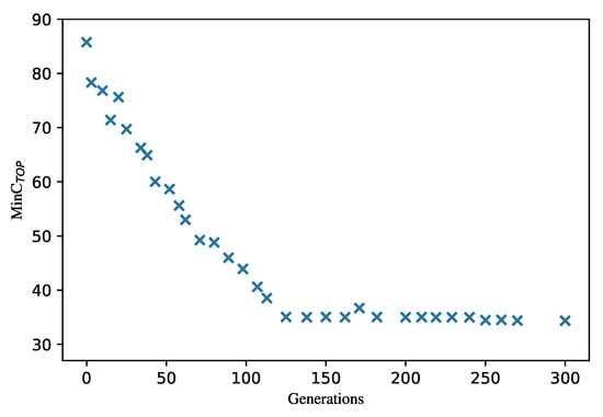
Figure 2.
The convergence of Min with the increase in generations.

Table 5.
The optimized risk of basic events after maintenance.

Table 6.
The solution of the singe-objective optimization model.
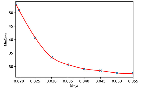
Figure 3.
The solution of the singe-objective optimization model.
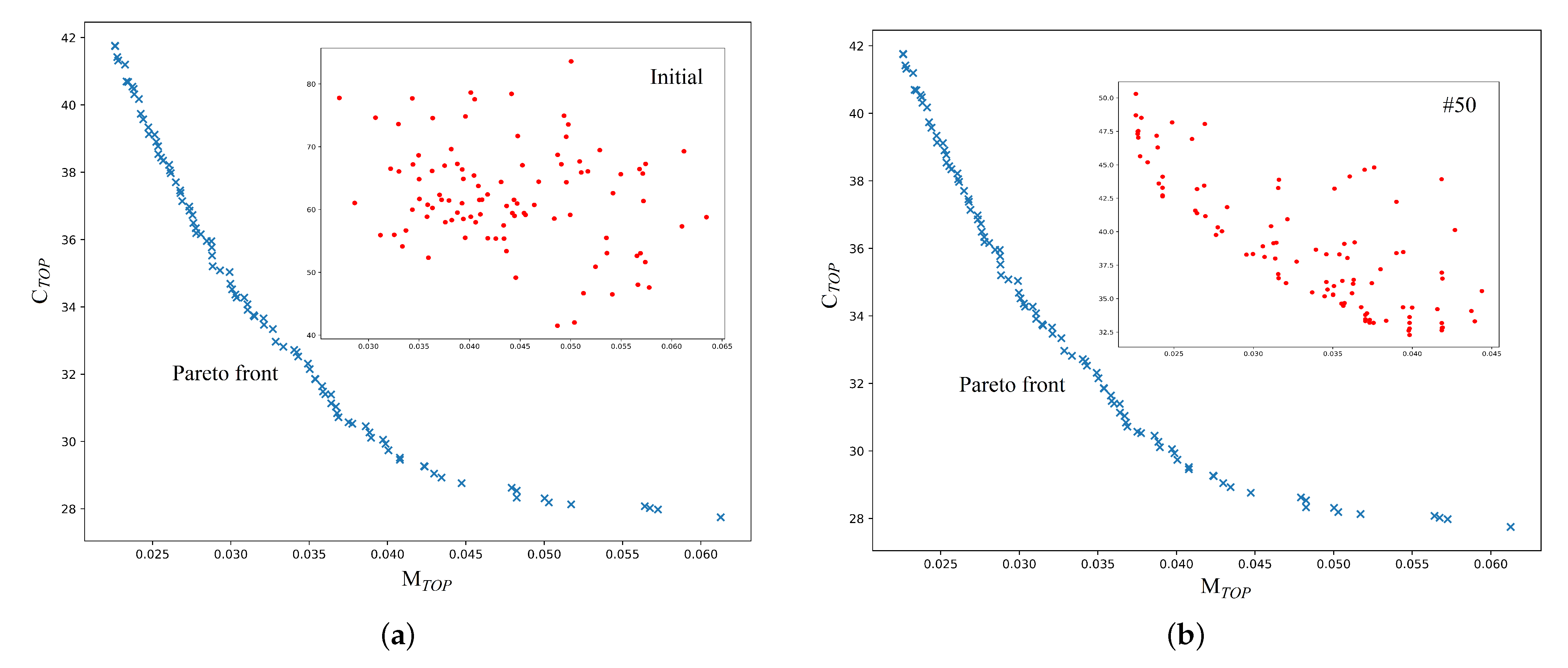
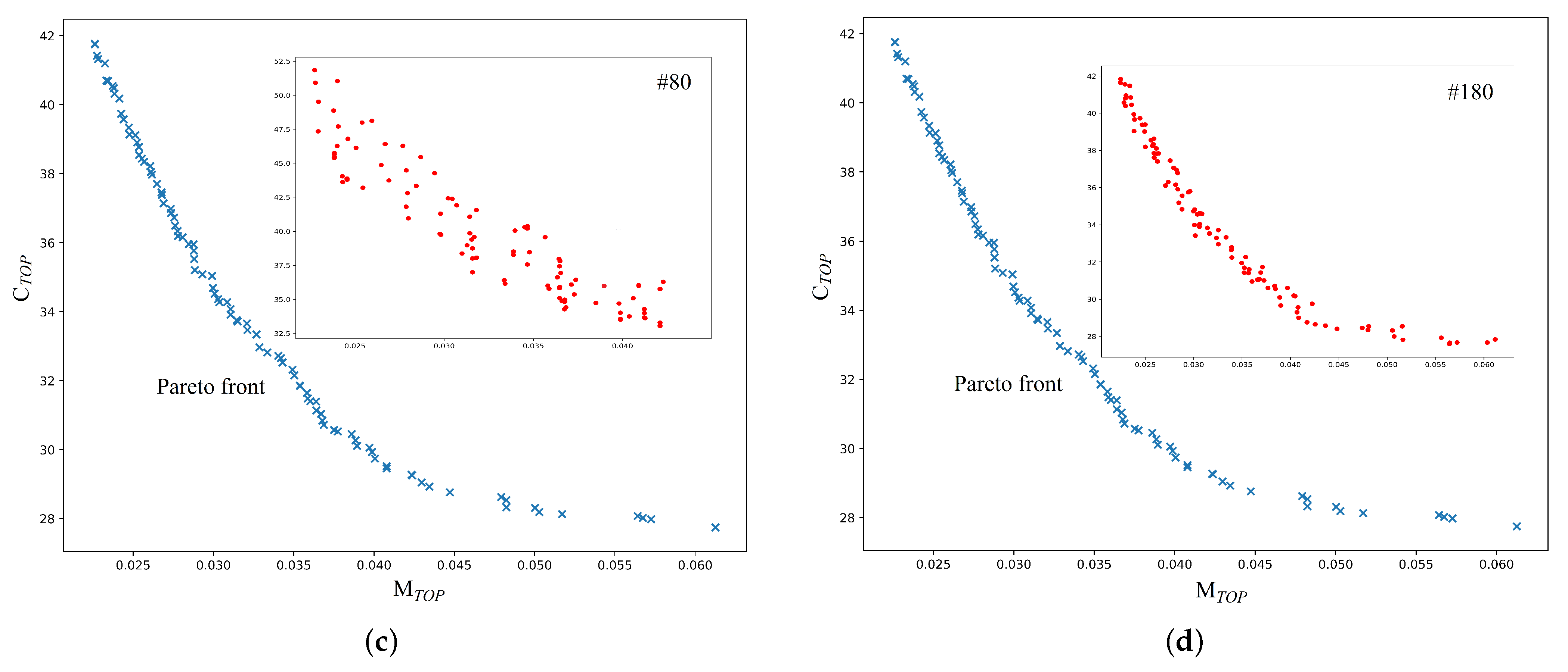
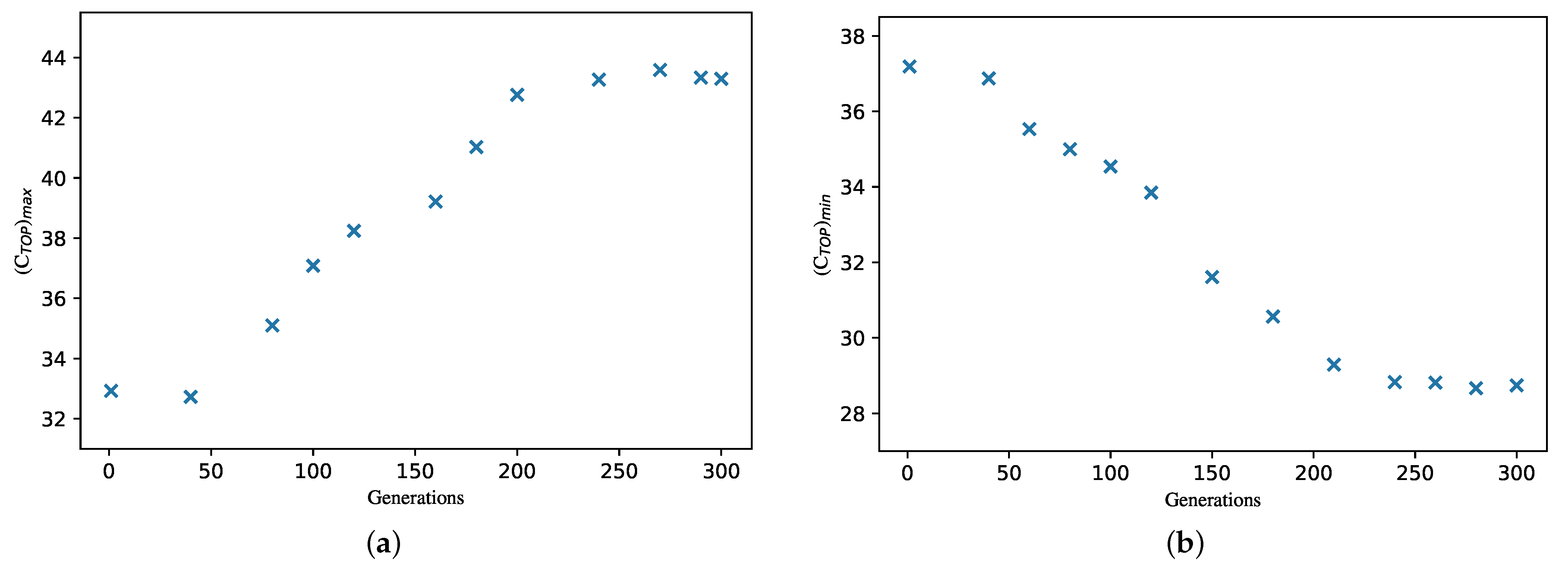
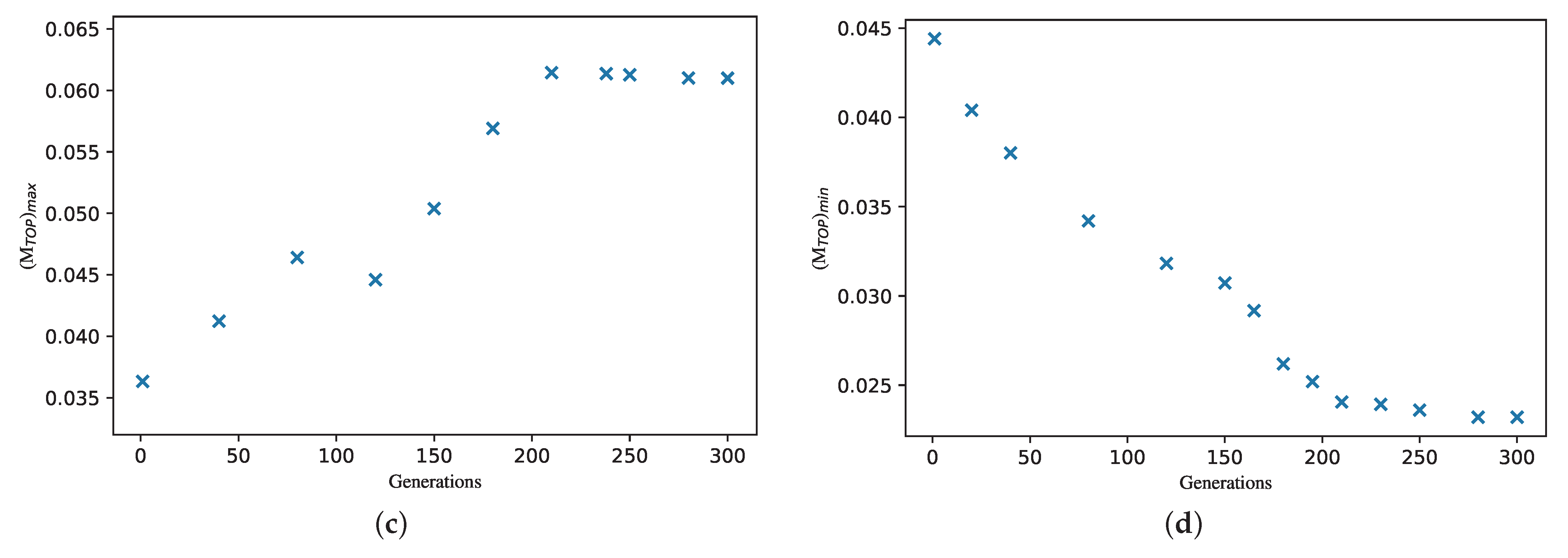
The multiobjective optimization Model (10) can be solved by the NSGA-II described in Appendix A.2. The key parameters of the NSGA-II were assigned as follows: the population size is 100, the crossover probability is 0.8, and the mutation probability is 0.04. Figure 4 shows a comparison between the Pareto front and the solutions of the initial population, 50th-generation population, 80th-generation population, and 180th-generation population. The values of and almost converge when the number of generations reaches 180. The converge maximum and minimum values of and are used to construct the ranges of the Pareto front.
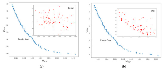
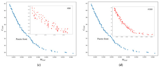
Figure 4.
Convergence process of Pareto optimal solution. The solution of (a) initial population; (b) 50th-generation population; (c) 80th-generation population; (d) 180th-generation population.
As shown in Figure 4 and Figure 5, the maximum and minimum values of and converge when the number of generations reaches 300. So, the number of generations was specified as 300 to ensure the Pareto front converged. Table 7 shows the Pareto optimal solutions on the Pareto front. It is up to the decision maker to adopt a Pareto optimal solution that lies on this Pareto front.
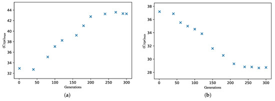

Figure 5.
The ranges of and with the number of generations: (a) maximum value of ; (b) minimum value of ; (c) maximum value of ; (d) minimum value of .

Table 7.
The Pareto optimal solutions on the Pareto front.
The optimization results provide the theoretical basis for practitioners to guarantee the safety of subsea production systems when they do not have sufficient data, which can help practitioners determine the preliminary funds need required in consideration of the system risk and give the maintenance degree of basic events.
5. Conclusions
It is difficult to obtain operation and maintenance data of subsea production systems, and the obtained data are often interpreted by experts. Therefore, evaluations of leakage risk based on the traditional fault tree analysis method are limited. Although the fuzzy fault tree is also used to evaluate system risk under incomplete information, it often produces conflicting evaluation results because the possibility measure does not have a duality property. In this study, the belief degrees of occurrence of basic events were measured with an uncertain measure. Then, the leakage risk of a subsea production system was evaluated with uncertain fault tree analysis. Furthermore, optimization models were established to optimize the leakage risk and maintenance cost of a subsea production system. The specific contributions of this study are as follows:
- (1)
- The belief degrees of the occurrence of basic events evaluated by experts are measured with an uncertain measure. A risk assessment method for complex systems with insufficient data was proposed based on uncertain fault tree analysis.
- (2)
- Two general optimization models were established for complex systems with insufficient data, in which the system risk is evaluated by an uncertain fault tree. GA and NSGA-II were applied to solve the two optimization models, separately.
- (3)
- The leakage risk of the subsea production system was evaluated with the proposed risk assessment method. Based on the findings, two optimization models were proposed to optimize the leakage risk and maintenance cost of a subsea production system, and the optimization results were discussed.
In future research, the proposed risk assessment method and optimization models will be used in the risk assessment and optimization problems for other complex systems with insufficient data.
Author Contributions
Conceptualization, J.Z. and Y.L.; methodology, L.M.; software, Y.S.; project administration, Y.L.; resources, Y.L. and J.Z.; data curation, Y.L. and L.M.; writing—original draft, L.M.; validation, Y.S. and X.S.; writing—review and editing, J.Z. and Y.L.; funding acquisition, Y.L. and J.Z. All authors have read and agreed to the published version of the manuscript.
Funding
This study was supported by the Humanities and Social Sciences Foundation of the Ministry of Education (Youth Fund) grant No. 18YJC630108 and the Scientific Research Project of Tianjin Education Commission grant No. 2019KJ233.
Institutional Review Board Statement
Not applicable.
Informed Consent Statement
Not applicable.
Data Availability Statement
The data that support the findings of this study are available from https://doi.org/10.1016/j.ress.2018.12.030, (accessed on 27 December 2018) and https://doi.org/10.1016/j.joes.2017.11.005, (accessed on 5 December 2017).
Conflicts of Interest
The authors declare no conflict of interest.
Appendix A
Appendix A.1. The Steps of GA
Step 1: Initialization
For each basic event , is generated by
in which is a random number generated between 0 and 1; and are the minimum and maximum values of , , respectively. The chromosome is constituted by . Then, k chromosomes are generated; the jth risk of basic event is denoted by , , .
Step 2: Calculate the risk of the top event
According to the fault tree structure of the subsea production system, the risk of the top event is calculated with Theorem 1. Then, the k risk of the top event is obtained, denoted by .
Step 3: Calculate the total maintenance cost
If , , the total maintenance cost can be calculated with Equation (3).
If , , proceed to Step 4.
Step 4: Selection
Calculate the average value
Compare with , if , then , , which is greater than , is selected. If , then , , which is less than , is selected.
Step 5: Crossover
For each basic event , two individuals and are randomly selected; random numbers p and q between 0 and 1 are generated. Then, new individuals are generated by
and
in which , and .
Replace and with and , respectively.
Step 6: Mutation
The individuals and locations to be mutated are randomly selected.
Appendix A.2. Steps of NSGA-II
Step 1: Initialization
For each basic event , is generated by
in which is a random number generated between 0 and 1; and are the minimum and maximum values of , , respectively. The chromosome is constituted by . Then, k chromosomes are generated; the jth risk of basic event is denoted by , , .
Step 2: Fast nondominated sort
Calculate the objective functions and with Equations (7) and (3), respectively. Arrange these chromosomes by using the fast nondominated sorting approach and arrive at the set .
Step 3: Crossover
Randomly select individuals and , to generate new individuals by
and
in which
where is a random number in [0,1], and is a distribution index.
Step 4: Mutation
The individuals who undergo mutation are randomly selected with probability p, and the new individuals after the mutation are generated by
in which
where is a random number in the interval [0,1]; is the distribution index, and are generated by
Then, k new chromosomes are generated, denoted by .
Step 5: Elite retention strategy
Combine and to construct 2k chromosome set, denoted by . Compute the objective functions and of with Equations (7) and (3), respectively. Rearrange the chromosome set and retain the top k chromosomes as chromosome set . Rename by , and proceed to Step 3 until the end of Step 5. The chromosomes construct the near-optimal Pareto front.
References
- Faddoul, R.; Raphael, W.; Chateauneuf, A. Maintenance optimization of series systems subject to reliability constraints. Reliab. Eng. Syst. Saf. 2018, 180, 179–188. [Google Scholar] [CrossRef]
- Hong, C.; Estefen, S.F.; Wang, Y.X.; Lourenco, M.I. An integrated optimization model for the layout design of a subsea production system. Appl. Ocean. Res. 2018, 77, 1–13. [Google Scholar] [CrossRef]
- Liu, X.Q.; Zheng, J.; Fu, J.J.; Ji, J.Q.; Chen, G.M. Multi-level optimization of maintenance plan for natural gas pipeline systems subject to external corrosion. J. Nat. Gas Sci. Eng. 2018, 50, 64–73. [Google Scholar] [CrossRef]
- Ma, X.Y.; Liu, B.; Yang, L.; Peng, R.; Zhang, X.D. Reliability analysis and condition-based maintenance optimization for a warm standby cooling system. Reliab. Eng. Syst. Saf. 2020, 193, 106588. [Google Scholar] [CrossRef]
- Yousefi, N.; Coit, D.W.; Song, S.L.; Feng, Q.M. Optimization of on-condition thresholds for a system of degrading components with competing dependent failure processes. Reliab. Eng. Syst. Saf. 2019, 192, 106547. [Google Scholar] [CrossRef]
- Zadeh, L.A. Fuzzy sets. Inf. Control 1965, 8, 338–353. [Google Scholar] [CrossRef]
- Mortazavi, A. A new fuzzy strategy for size and topology optimization of truss structures. Appl. Soft Comput. J. 2020, 93, 106412. [Google Scholar] [CrossRef]
- Sayyaadi, H.; Baghsheikhi, M. Developing a novel methodology based on the adaptive neuro-fuzzy interference system for the exergoeconomic optimization of energy systems. Energy 2018, 164, 218–235. [Google Scholar] [CrossRef]
- Yang, H.F.; Zhu, Z.J.; Li, C.; Li, R.R. A novel combined forecasting system for air pollutants concentration based on fuzzy theory and optimization of aggregation weight. Appl. Soft Comput. J. 2020, 87, 105972. [Google Scholar] [CrossRef]
- Zhou, J.; Han, Y.L.; Liu, J.; Pantelous, A.A. New approaches for optimizing standby redundant systems with fuzzy lifetimes. Comput. Ind. Eng. 2018, 123, 263–277. [Google Scholar] [CrossRef]
- Liu, B.D. Why is there a need for uncertainty? J. Uncertain Syst. 2012, 6, 3–10. [Google Scholar]
- Liu, B.D. Uncertainty Theory, 2nd ed.; Springer: Berlin, Germany, 2007. [Google Scholar]
- Liu, B.D. Uncertainty Theory: A Branch of Mathematics for Modeling Human Uncertainty; Springer: Berlin, Germany, 2010. [Google Scholar]
- Liu, Y.; Zhao, J.Y.; Qu, Z.G.; Wang, L. Structural reliability assessment based on subjective uncertainty. Int. J. Comput. Methods 2021, 18, 2150046. [Google Scholar] [CrossRef]
- Gao, Y. Uncertain inference control for balancing an inverted pendulum. Fuzzy Optim. Decis. Mak. 2012, 11, 481–492. [Google Scholar] [CrossRef]
- Hu, L.H.; Kang, R.; Pan, X.; Zuo, D.J. Risk assessment of uncertain random system-level-1 and level-2 joint propagation of uncertainty and probabiltiy in fault tree analysis. Reliab. Eng. Syst. Saf. 2020, 198, 106874. [Google Scholar] [CrossRef]
- Zu, T.P.; Kang, R.; Wen, M.L. Graduation formula: A new method to construct belief reliability distribution under epistemic uncertainty. J. Syst. Eng. Electron. 2020, 31, 626–633. [Google Scholar]
- Ke, H.; Yao, K. Block replacement policy with uncertain lifetimes. Reliab. Eng. Syst. Saf. 2016, 148, 119–124. [Google Scholar] [CrossRef]
- Liu, Y.; Li, X.Z.; Liu, Y.L. The bounds of premium and optimality of stop loss insurance under uncertain random environments. Insur. Math. Econ. 2015, 64, 273–278. [Google Scholar] [CrossRef]
- Zhang, B.; Peng, J. Uncertain programming model for uncertain optimal assignment problem. Appl. Math. Model. 2013, 37, 6458–6468. [Google Scholar] [CrossRef]
- Li, B.; Sun, Y.F.; Aw, G.; Teo, K.L. Uncertain portfolio optimization problem under a minimax risk measure. Appl. Math. Model. 2019, 76, 274–281. [Google Scholar] [CrossRef]
- Li, Y.C.; Peng, R.; Kucukkoc, I.; Tang, X.W.; Wei, F. System reliability optimization for an assembly line under uncertain random environment. Comput. Ind. Eng. 2020, 146, 106540. [Google Scholar] [CrossRef]
- Wen, M.L.; Han, Q.; Yang, Y.; Kang, R. Uncertain optimization model for multi-echelon spare parts supply system. Appl. Soft Comput. 2017, 56, 646–654. [Google Scholar] [CrossRef]
- Li, Y.C.; Hu, X.F.; Tang, X.W.; Kucukkoc, I. Type-1 U-shaped assembly line balancing under uncertain task time. IFAC Pap. Online 2019, 52, 992–997. [Google Scholar] [CrossRef]
- Guo, L.H.; Fun, J.J.; Wen, M.L.; Kang, R. Joint optimization of LORA and spares stocks considering corrective maintenance time. J. Syst. Eng. Electron. 2015, 26, 85–95. [Google Scholar] [CrossRef]
- Andrews, J.; Bartlett, L. Genetic algorithm optimization of a firewater deluge system. Qual. Reliab. Eng. Int. 2003, 19, 39–52. [Google Scholar] [CrossRef]
- Pattison, R.; Andrews, J. Genetic algorithms in optimal safety system design. Proc. Inst. Mech. Eng. Part E J. Process Mech. Eng. 1999, 213, 187–197. [Google Scholar] [CrossRef]
- Cui, D.; Wang, G.Q.; Lu, Y.P.; Sun, K.K. Reliability design and optimization of the planetary gear by a GA based on the DEM and Kriging model. Reliab. Eng. Syst. Saf. 2020, 203, 107074. [Google Scholar] [CrossRef]
- Ardakan, M.A.; Rezvan, M.T. Multi-objective optimization of reliability-redundancy allocation problem with cold-standby strategy using NSGA-II. Reliab. Eng. Syst. Saf. 2018, 172, 225–238. [Google Scholar] [CrossRef]
- Bhattacharyya, S.K.; Cheliyan, A.S. Optimization of a subsea production system for cost and reliability using its fault tree model. Reliab. Eng. Syst. Saf. 2019, 185, 213–219. [Google Scholar] [CrossRef]
- Wang, W.; Sun, L.P.; Bai, Y. Investigation on subsea production systems. China Offshore Platf. 2019, 24, 41–45. [Google Scholar]
- Cheliyan, A.S.; Bhattacharyya, S.K. Fuzzy fault tree analysis of oil and gas leakage in subsea production systems. J. Ocean. Eng. Sci. 2018, 3, 38–48. [Google Scholar] [CrossRef]
- Liu, B.D. Some research problems in uncertainty theory. J. Uncertain Syst. 2009, 3, 3–10. [Google Scholar]
Disclaimer/Publisher’s Note: The statements, opinions and data contained in all publications are solely those of the individual author(s) and contributor(s) and not of MDPI and/or the editor(s). MDPI and/or the editor(s) disclaim responsibility for any injury to people or property resulting from any ideas, methods, instructions or products referred to in the content. |
© 2023 by the authors. Licensee MDPI, Basel, Switzerland. This article is an open access article distributed under the terms and conditions of the Creative Commons Attribution (CC BY) license (https://creativecommons.org/licenses/by/4.0/).


