Article

Condition-Based Maintenance Optimization Method Using Performance Margin

1
School of Reliability and Systems Engineering, Beihang University, Beijing 100191, China
2
The Key Laboratory on Reliability and Environmental Engineering Technology, Beihang University, Beijing 100191, China
3
School of Aeronautic Science and Engineering, Beihang University, Beijing 100191, China
*
Author to whom correspondence should be addressed.
Axioms 2023, 12(2), 168; https://doi.org/10.3390/axioms12020168
Submission received: 12 January 2023 / Revised: 3 February 2023 / Accepted: 4 February 2023 / Published: 7 February 2023
(This article belongs to the Special Issue Advances in Uncertain Optimization and Applications)

Abstract

:
As a maintenance strategy to reduce unexpected failures and enable safe operation, condition-based maintenance (CBM) has been widely used in recent years. The maintenance decision criteria of CBM in the literature mostly originate from statistical failure data or degradation states, few of which can directly and effectively reflect the current state and analyze condition monitoring data, maintenance measures, and reliability together at the same time. In this paper, we introduce the performance margin as a decision criterion of CBM. We propose a condition-based maintenance optimization method using performance margin. Considering a CBM optimization problem for a degrading and periodically inspected component, a newly developed performance margin degradation model is established when three different maintenance measures become involved. Maintenance measure effect factors, maintenance decision vectors, and maintenance measure threshold vectors are developed to update the degradation model. And to build a maintenance optimization model, both cost and loss related to maintenance decision problems and reliability obtained by performance margin have been taken into consideration. Finally, a numerical example is provided to illustrate the proposed optimization method.

1. Introduction

With the ongoing development of technology and the requirements of products, the complexity and cost of products are also increasing. Facing these advanced products, a proper maintenance strategy is an important means to improve the efficiency of safe operation, extend the service life, and reduce or avoid the impact due to failure. Hence, a condition-based maintenance (CBM) strategy has gradually gained increasing application value. CBM has been studied and applied to numerous areas, such as electronics [1,2], mechanics [3,4], wind turbines [5,6], the aerospace industry [7], nuclear power [8], the railway industry [9], seaports [10], etc.
Scientific, practical, and comprehensive maintenance decision criteria are the basis for CBM. Existing decision criteria of maintenance strategies can be categorized into two types: failure-related criteria and degradation-related criteria. Failure-related criteria originate from statistical failure data, for example, failure rate [11], probability density function (PDF) [12], mean time to failure (MTTF) and residual useful life (RUL) [13,14]. Such criteria are mostly the description of the product after failure and are not suitable for CBM monitoring of current working conditions. Additionally, these criteria require sufficient failure data, but for high-reliability and long-life products, failure data is difficult to obtain. Therefore, the actual operation condition of the product cannot be accurately reflected. Degradation-related criteria, for instance, degradation states [15,16], degradation levels [17], and deterioration rate [18], are widely used for CBM. They basically solved the two problems of failure-related criteria, but there are still some imperfections. On the one hand, the degradation-related criteria tend to focus on the condition-monitoring data (e.g., temperature, humidity, pressure, vibration, acoustic, etc.) and mostly neglect the data for maintenance and other relative measures (e.g., installation, breakdown, overhaul, minor repair, preventive maintenance, oil change, etc.). However, the data for maintenance and other relative measures are very important in CBM because to better assess the products’ performance and condition, what happened and what was done during the whole life cycle should be considered. On the other hand, when using the degradation-related criteria, the reliability of products is often assessed by the first hitting time (FHT) or the remaining useful life (RUL)/ mean residual life (MRL) in terms of FHT. The derivation processes of the distribution functions of FHT and RUL/MRL are mostly complex, and sometimes the approximate method is used to find the solution. Under such circumstances, the degradation-related criteria seem to be insufficient to describe the conditions of products.
Compared to CBM strategies using the above two types of criteria, a strategy based on performance margin can be more effective. First of all, the performance margin can reflect the current condition of the product. Performance margin is the margin that is reserved for performance parameters, and the conditions required for a product to perform its required functions depend on its performance margin. Secondly, performance margin can also determine and then be influenced by maintenance decisions and other relative measures. The ability of a product to maintain or restore its required state depends on its current performance margin, measures such as maintenance and replacement react to performance margin, as well. Thus, it is possible to analyze maintenance and condition monitoring data together by performance margin. Furthermore, performance margin can be used in reliability analysis more conveniently. According to the margin-based reliable principle of belief reliability [19], the performance margin determines how reliable the object is. Performance margin is essentially a certain distance between the performance parameter and the performance threshold, it can be a direct bridge from the condition of products to the reliability metric. Additionally, numerous factors, including the environment, the inner structure, and multiple failure mechanisms used in reliability analysis can be considered when performance margin is used to describe the condition of products [20,21]. These all allow the CBM strategy based on performance margin to assess reliability effectively, which is beneficial to control the risk.
Therefore, we introduce the performance margin into the degradation model in this article to describe the monitored conditions. Taking performance margin as a criterion has the following advantages:
  • Proceed from the current states and conditions of products directly;
  • Maintenance and other relative measures can be analyzed comprehensively with condition monitoring data;
  • Be able to assess reliability more effectively.
In this paper, we develop a condition-based maintenance optimization method using performance margin. The degradation and recovery of a single component are modeled by a multi-stage Wiener process. The component is assumed to undergo periodic inspections, and conditions can only be totally be revealed at inspections. The performance margin detected at each inspection will determine the corresponding type of maintenance measures. Different maintenance measures, including preventive maintenance, preventive replacement, and replacement after failure can only be taken at the inspections and can cause different degrees of restoration of performance margin. After completion of maintenance measures, the component resumes operation without changing the original drift of performance margin degradation. The final purpose is to find the optimal inspection intervals and make reasonable maintenance decisions to control the cost and ensure reliability.
The remainder of this article is organized as follows. In Section 2, we present the establishment of the performance margin degradation model. In Section 3, we build an optimization model of maintenance. Section 4 provides a numerical case, including a discussion of the results. Conclusions are addressed in Section 5.2, Framework and Symbols.

2. Framework and Symbols

2.1. Framework

The framework of the condition-based maintenance optimization method using performance margin is proposed in Figure 1. Firstly, the origin performance margin degradation model with uncertainty is established based on the Wiener process. Then, a multi-stage Wiener process is proposed to characterize the maintenance-involved degradation of the performance margin. To determine the initial value of the performance margin at each stage, the maintenance measure threshold vector and maintenance measure decision vector are employed and the transition of the performance margin is modeled based on the effect of maintenance and replacement. Finally, the optimization model of the maintenance decision problem is constructed.

2.2. Symbols

B ( t ) : standard Wiener process at time t ;
C ¯ : overall cost per time;
C D T : total loss in unplanned downtime after failure;
c D T : maximum loss of any kind of unplanned downtime, a constant;
C D T 0 : the basic loss of any kind of unplanned downtime after failure;
C D T m a x : the maximum allowable total loss in unplanned downtime after failure, a constant;
C P d M : total cost of preventive maintenance;
c P d M : maximum cost of single preventive maintenance, a constant;
C P d R : total cost of preventive replacement;
C P T : total cost of inspections;
c P T : cost of a single inspection, a constant;
C R P : total cost of replacement after failure;
c R P : cost of a single replacement, a constant;
C Z : overall cost;
k P d M , C : cost coefficient of preventive maintenance, a constant;
k t h , C : loss coefficient in unplanned downtime, a constant;
m 0 : initial value of performance margin at time t = 0 ;
m P d M : preventive maintenance threshold, a constant;
m P d R : preventive replacement threshold, a constant;
m ( t ) : degradation function of performance margin;
m i ( t ) : degradation function of performance margin at i t h inspection;
m i ( t ) : degradation function of performance margin after maintenance at i t h inspection;
m i ( t i ) : the value of performance margin after maintenance at the end of i t h inspection (time t i ), which also means the initial value of performance margin at ( i + 1 ) t h inspection, i = 1 , 2 , , N ;
N : total number of inspections, a constant;
n i : the number of maintenance procedures by the i t h inspection (time t i );
p : degradation coefficient of maintenance effect factor, a constant;
r : maintenance effect factor;
R 0 : the minimum allowable reliability, a constant;
R i : the reliability at i t h inspection;
T i : the interval between ( i 1 ) t h inspection and i t h inspection, T i = t i t i 1 ;
t i : time point at end of the i t h inspection;
T Z : overall time;
λ : drift parameter, a constant;
μ : indicative function of preventive maintenance;
ν : indicative function of preventive replacement;
σ : diffusion parameter, a constant;
ω : indicative function of replacement after failure;

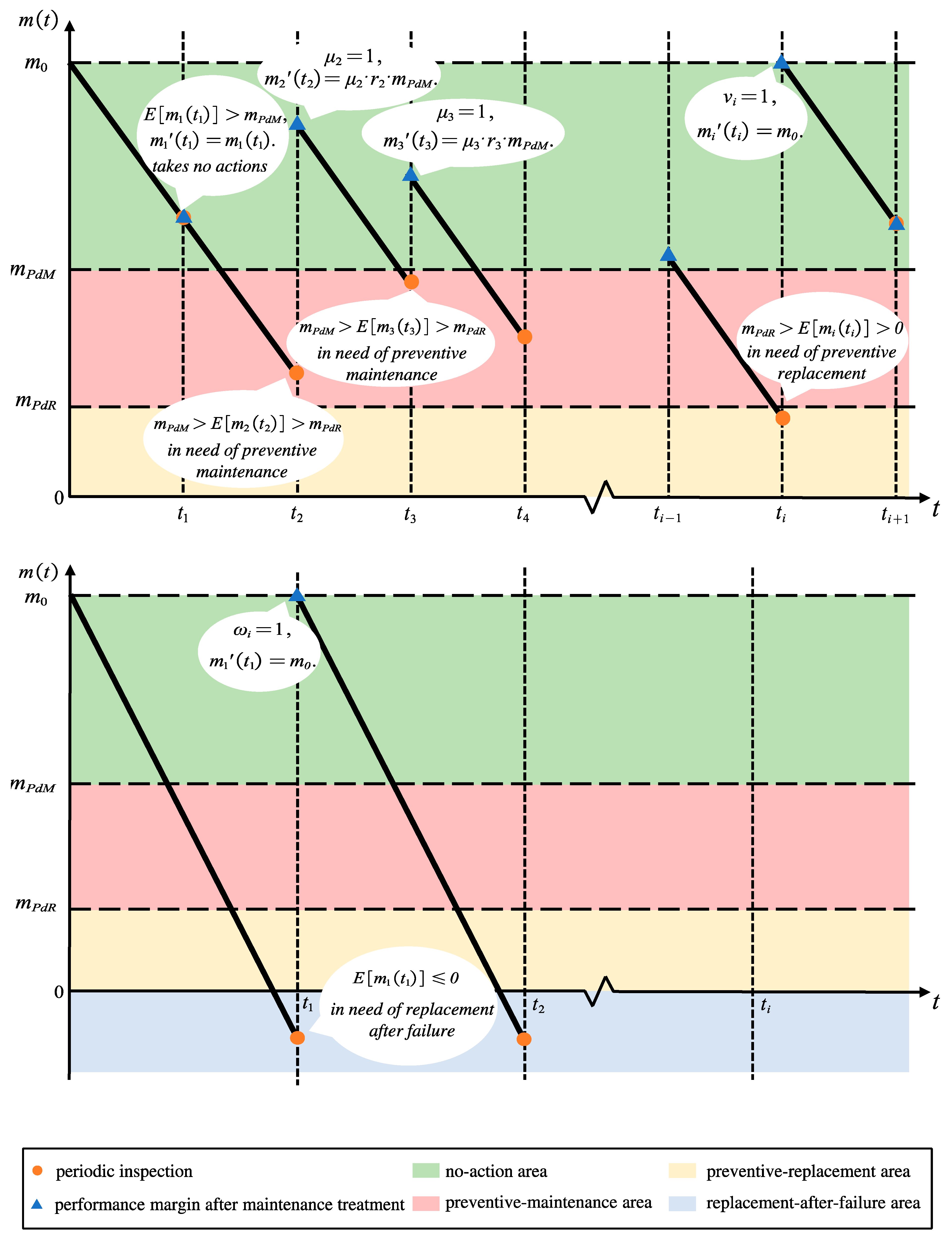
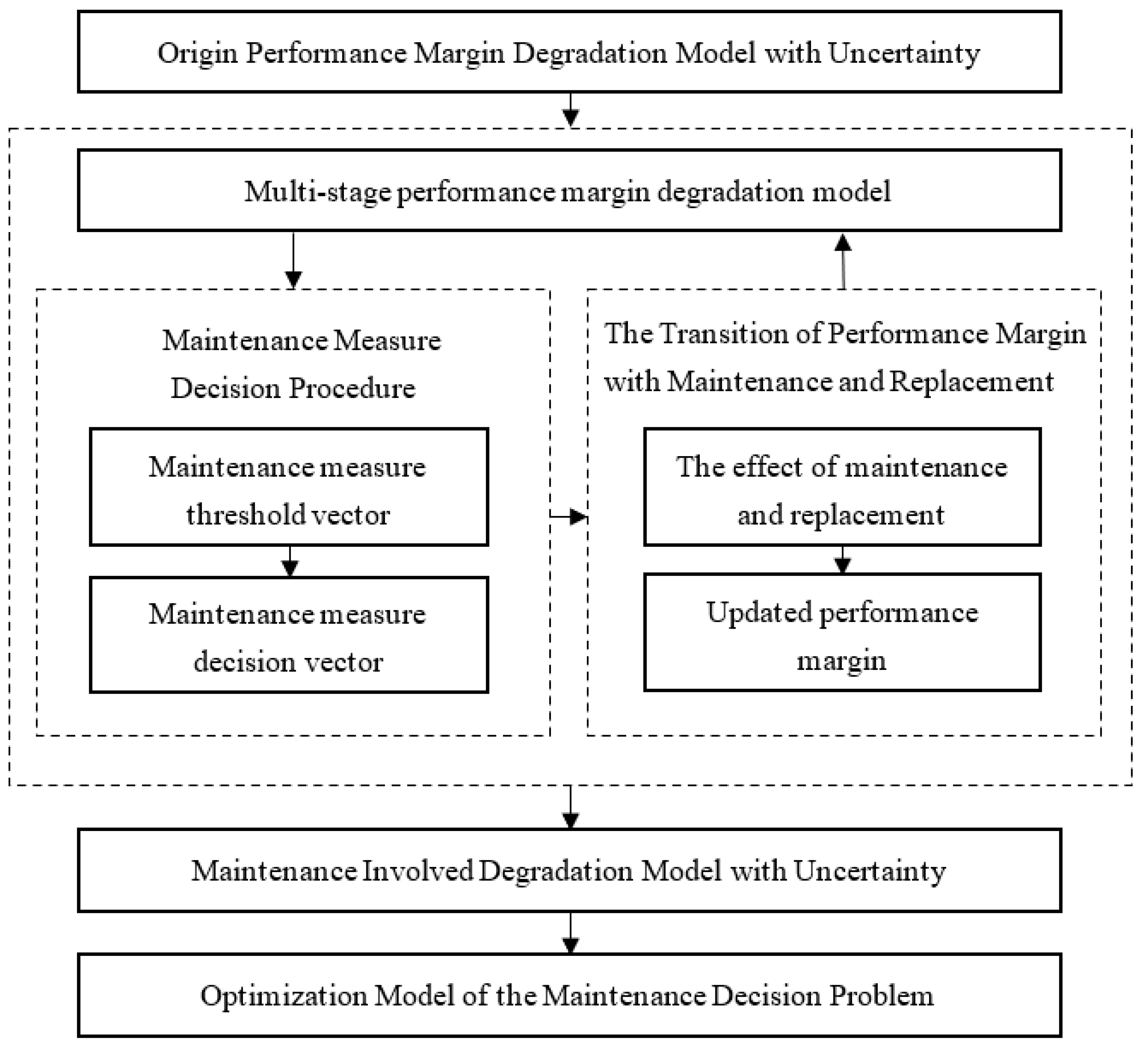
3. Performance Margin Degradation Model with Uncertainty

We consider a component whose performance margin is degrading and periodically inspected, multiple types of maintenance measures will be conducted according to the performance margin. We divide the establishment of the performance margin degradation model into two steps: first, building an origin model to describe the degradation process without any maintenance; and second, updating the degradation model when different maintenance measures become involved.

3.1. Origin Degradation Model with Uncertainty

The Wiener process is widely employed to describe degradation processes that are characterized by a gradual drift of the mean value [22]. In this paper, the degradation of performance margin is assumed to be an additive accumulation and expressed by the Wiener process. Let m ( t ) be the degradation function of performance margin function, and degradation follows a linear drift Wiener process { m ( t ) : t 0 } :
m ( t ) = m 0 [ λ t + σ B ( t ) ] .

3.2. Maintenance-Involved Degradation Model with Uncertainty

When maintenance measures are involved, the performance margin will be updated, and the degradation of performance margin will be changed accordingly. Therefore, we built a maintenance-involved degradation model of performance margin to better describe this process, and Figure 2 illustrates this maintenance-involved degradation process.

3.2.1. Multi-Stage Wiener Process

Assuming that the component is inspected at the regular time t i ( i = 1 , 2 , , N ), a multi-stage Wiener process is proposed to characterize the maintenance-involved degradation of performance margin. The initial value of performance margin at stage i is also the value after maintenance measure at stage i + 1 . According to formula (1), the degradation function of the performance margin at ( i + 1 ) t h inspection can be given as:
m i + 1 ( t ) = m i ( t i ) [ λ ( t t i ) + σ B ( t t i ) ] .

3.2.2. Maintenance Measure Decision Procedure

The choice of maintenance or replacement fundamentally depends on the condition (represented by performance margin) before maintenance measures. To model the procedure for the maintenance measure decision, we developed a maintenance measure decision vector and a maintenance measure threshold vector. The relationship of the above vectors is actually the decision procedure for the maintenance measure.
The maintenance measure decision vector is introduced as follows:
M D i = ( μ i , ν i , ω i ) .
The maintenance measure threshold vector is introduced as follows:
M t h = ( m P d M , m P d R , 0 ) ,
where m P d M > m P d R > 0 .
A component is considered in need of preventive maintenance when its performance margin decreases to m P d M . The indicative function of preventive maintenance can be expressed as:
μ i = { 1 , i f   m P d M > E [ m i ( t i ) ] > m P d R 0 ,   e l s e .
A component is considered in need of preventive replacement when its performance margin decreases to m P d R . The indicative function of preventive replacement can be expressed as:
ν i = { 1 ,   i f   m P d R > E [ m i ( t i ) ] > 0 0 ,   e l s e .
A unit is considered failed and in need of replacement when its performance margin decreases to 0, and the indicative function of replacement after failure can be expressed as:
ω i = { 1 ,   i f   E [ m i ( t i ) ] 0 0 ,   e l s e .

3.2.3. The Transition of Performance Margin with Maintenance and Replacement

In this article, the initial value of performance margin at ( i + 1 ) t h inspection is considered to be concerned with the maintenance measure that is used at the end of i t h inspection (time t i ).
Here, we introduce a maintenance effect factor, r , to better describe the restoration effect of the performance margin after maintenance. The initial value of the performance margin at the ( i + 1 ) t h inspection can be expressed as:
m i ( t i ) = r i m P d M .
This effect factor, r , represents the extent to which the performance margin can revert back. In this paper, we consider the number of maintenance procedures, and assume that the more maintenance procedures that are carried out, the worse the maintenance effects are. Maintenance effect factor r i can be expressed as:
r i = 1 + p / n i .
Since maintenance must play a role in recovery, we have:
m 0 > m i ( t i ) > m i ( t i ) > m P d R .
Thus, the number of maintenance procedures needs to satisfy the following equation:
n i > p m 0 m P d M 1 .
Also, the initial value of performance margin at ( i + 1 ) t h inspection is considered to be concerned with replacement. If a preventive replacement or replacement after failure is carried out, the initial value of performance margin at ( i + 1 ) t h inspection can be restored to the initial value of the performance margin at time t = 0 , which can be expressed as:
m i ( t i ) = m 0 .
Therefore, the comprehensive expression of the updated initial value of performance margin at ( i + 1 ) t h inspection with maintenance and replacement can be expressed as:
m i ( t i ) = μ i r i m P d M + ν i m 0 + ω i m 0 + ( 1 μ i ) ( 1 ν i ) ( 1 ω i ) m i ( t i ) .
According to Section 3.2.2, when the maintenance measure is decided, the expression of the updated initial value of performance margin at ( i + 1 ) t h inspection can be simplified, as follows:
When the component is considered to be in need of preventive maintenance, we have M D i = ( 1 , 0 , 0 ) . Then Equation (13) can be transferred into Equation (8).
When the component is considered to be in need of preventive replacement, we have M D i = ( 0 , 1 , 0 ) . Then Equation (13) can be transferred into Equation (12).
When the component is considered to be in need of replacement after failure, we have M D i = ( 0 , 0 , 1 ) . Then Equation (13) can be transferred into Equation (12).
When the component is considered to be in need of no maintenance measures, we have M D i = ( 0 , 0 , 0 ) . Then Equation (13) can be transferred into m i ( t i ) , which means that the performance margin remains unchanged.

4. Optimization Model of the Maintenance Decision Problem

With the newly developed performance margin degradation model, we consider the cost of the maintenance decision problem. In this section, we elaborate on the detailed contents of the optimization model.

4.1. Indexes

  • Overall cost:
The overall cost of the optimization model consists of the cost of inspection, preventive maintenance, preventive replacement, replacement after failure, and loss in unplanned downtime after failure, and they can be expressed as followed.
(1)
The total cost of inspections:
C P T = N c P T ,
which is the product of the number of inspection times and the cost of a single inspection;
(2)
The total cost of preventive maintenance;
The cost of preventive maintenance increases with the decrease of maintenance performance margin. When the performance margin is approaching the preventive maintenance threshold, the cost of preventive maintenance is approaching zero, which can be expressed as:
C P d M = i = 1 N [ ( 1 ln m P d M ln E [ m i ( t i ) ] m P d M E [ m i ( t i ) ] E [ m i ( t i ) ] ) k P d M , C μ i ] c P d M .
(3)
The total cost of preventive replacement:
C P d R = i = 1 N ν i c R P ,
which is the product of the number of times of preventive replacement and the cost of a single replacement;
(4)
The total cost of replacement after failure:
C R P = i = 1 N ω i c R P ,
which is the product of the number of times of replacement after failure and the cost of a single replacement;
(5)
Loss in unplanned downtime after failure:
When the performance margin decreases to less than zero, unplanned downtime is generated. Once the unplanned downtime is generated, no matter how long it lasts, there is a basic loss. Additionally, the longer the unplanned downtime lasts, the more the performance margin deviates from zero, and the greater the loss, which can be expressed as:
C D T = i = 1 N [ C D T 0 + | E [ m i ( t i ) ] | k t h , C c D T ] ω i .
Therefore, the overall cost is expressed as:
C Z = C P T + C P d M + C P d R + C D T + C R P = N c P T + i = 1 N [ ( 1 ln m P d M ln E [ m i ( t i ) ] m P d M E [ m i ( t i ) ] E [ m i ( t i ) ] ) k P d M , C μ i ] c P d M + i = 1 N ν i c R P + i = 1 N ω i c R P + i = 1 N [ c D T 0 + | E [ m i ( t i ) ] | k t h , C c D T ] ω i .
2.
Reliability:
According to the margin-based reliable principle of belief reliability [19], performance margin, m , describes the distance between a performance parameter and its failure threshold. So, when m i ( t ) > 0 , the component can act normally, then the reliability at i t h inspection can be expressed as:
R i = P r { m i ( t ) > 0 } ,
which describes the probability that the component can act normally.
3.
Overall time:
In this paper, we only consider the working time of components, and neglect the time of inspection, preventive maintenance, preventive replacement, halt after failure, replacement after failure, etc. Therefore, the intervals between inspections are the working time of components, and the overall time can be expressed as:
T Z = i = 1 N T i ,
which is the sum of all the intervals between inspections.
4.
Overall cost per time:
The overall cost per time is the overall cost divided by the overall time, which can be expressed as:
C ¯ = C Z T Z ,
where C Z follows Equation (19) and T Z follows Equation (21).

4.2. Model

The overall cost per time is taken as the objective function, and the optimal inspection and maintenance policy is solved by this model. The model should also meet the following constraints: (1) the loss in unplanned downtime after failure should not exceed the maximum allowable value; (2) the reliability should exceed the minimum allowable value; and (3) the inspection interval should be non-negative. Therefore, the optimization model can be expressed as:
{ m i n   C = ( N c P T + i = 1 N [ ( 1 l n m P d M l n E [ m i ( t i ) ] m P d M E [ m i ( t i ) ] E [ m i ( t i ) ] ) k P d M , C μ i ] c P d M + i = 1 N ν i c R P + i = 1 N ω i c R P + i = 1 N [ c D T 0 + | E [ m i ( t i ) ] | k t h , C c D T ] ω i ) T Z s . t . i = 1 N [ C D T 0 + | E [ m i ( t i ) ] | k t h , C c D T ] ω i C D T m a x R i = P { m i ( t ) > 0 } R 0 T i 0

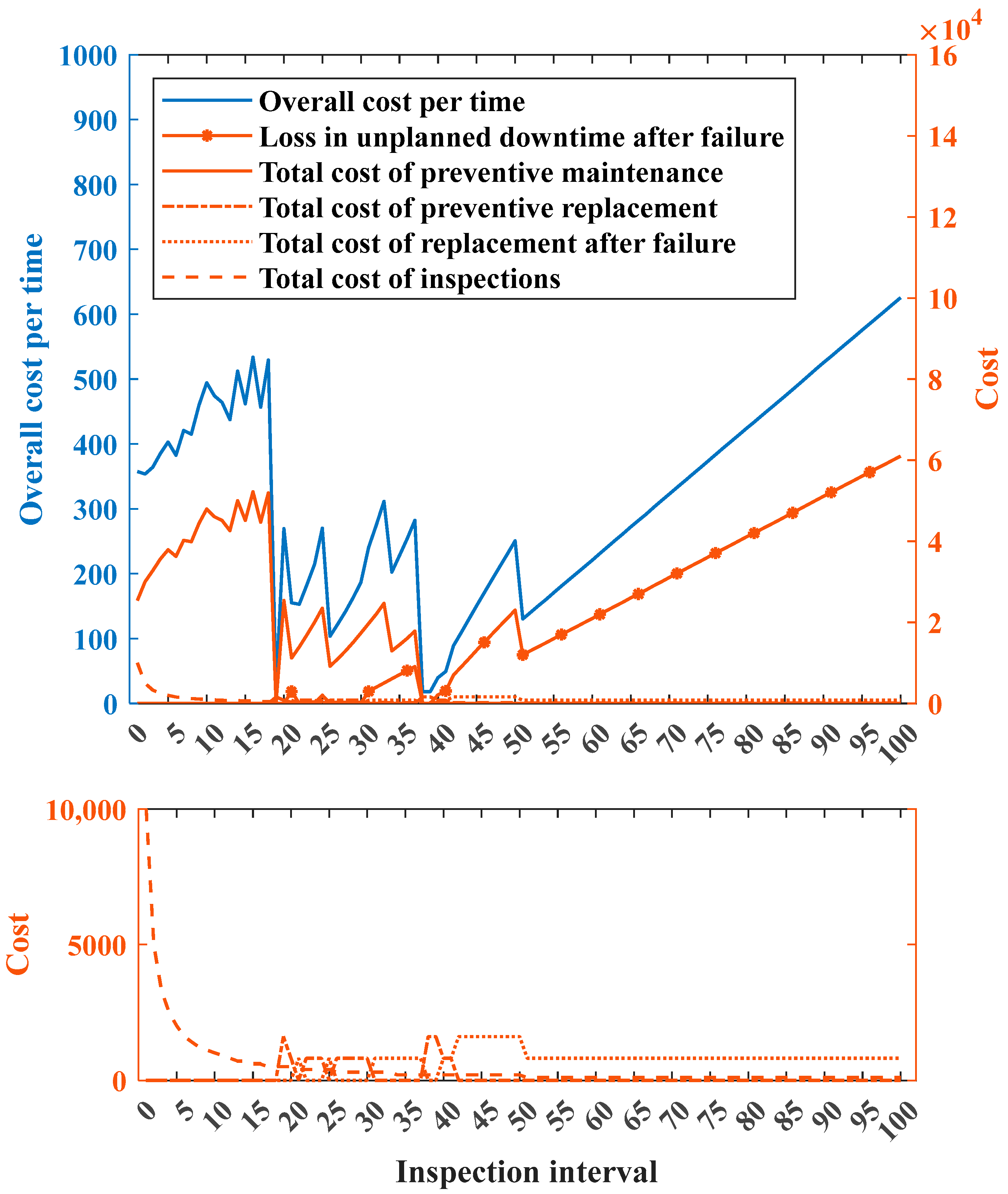
5. A Numerical Example

In this section, we use a numerical example to demonstrate the proposed optimization model; this example follows all of the mentioned assumptions.

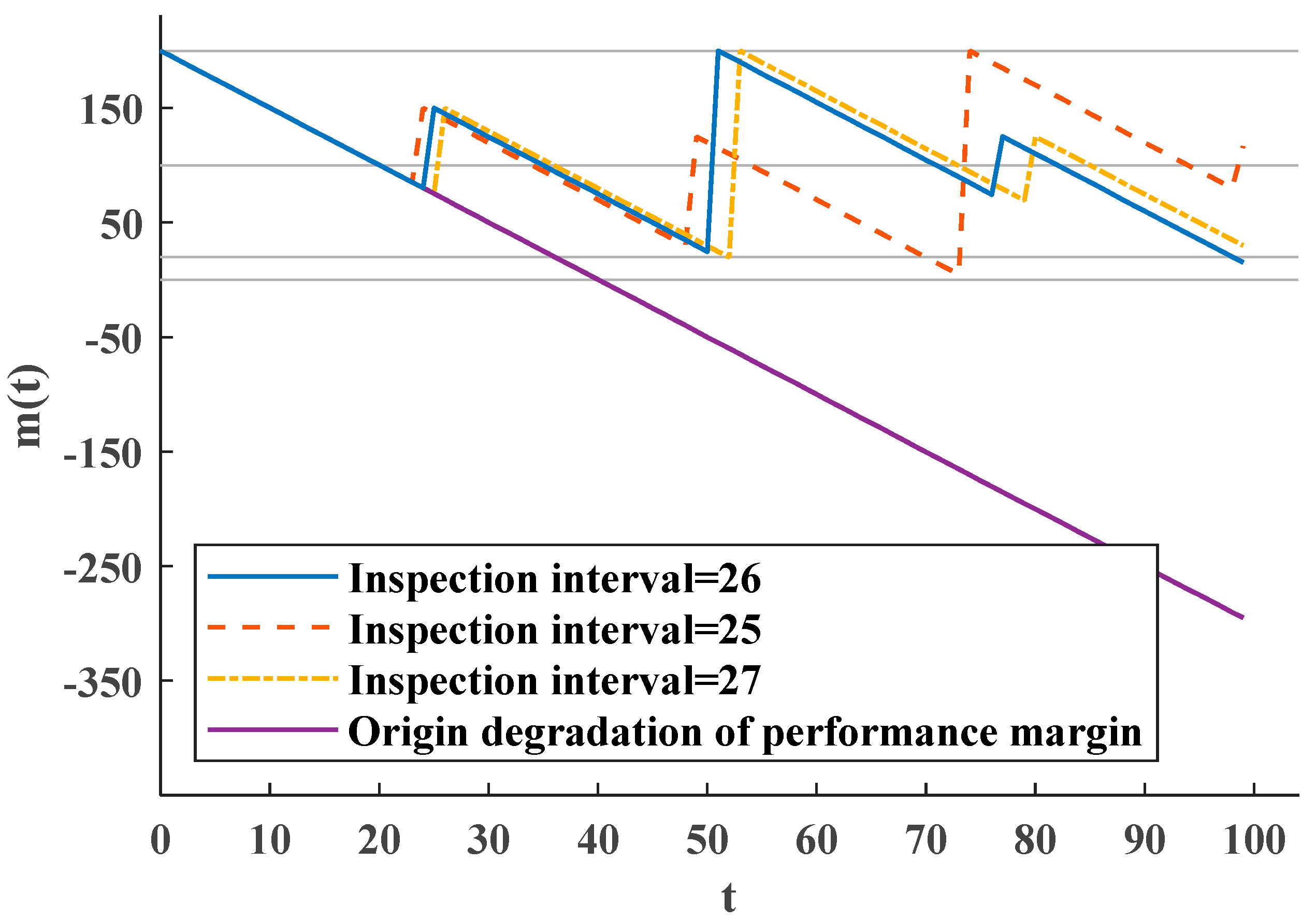
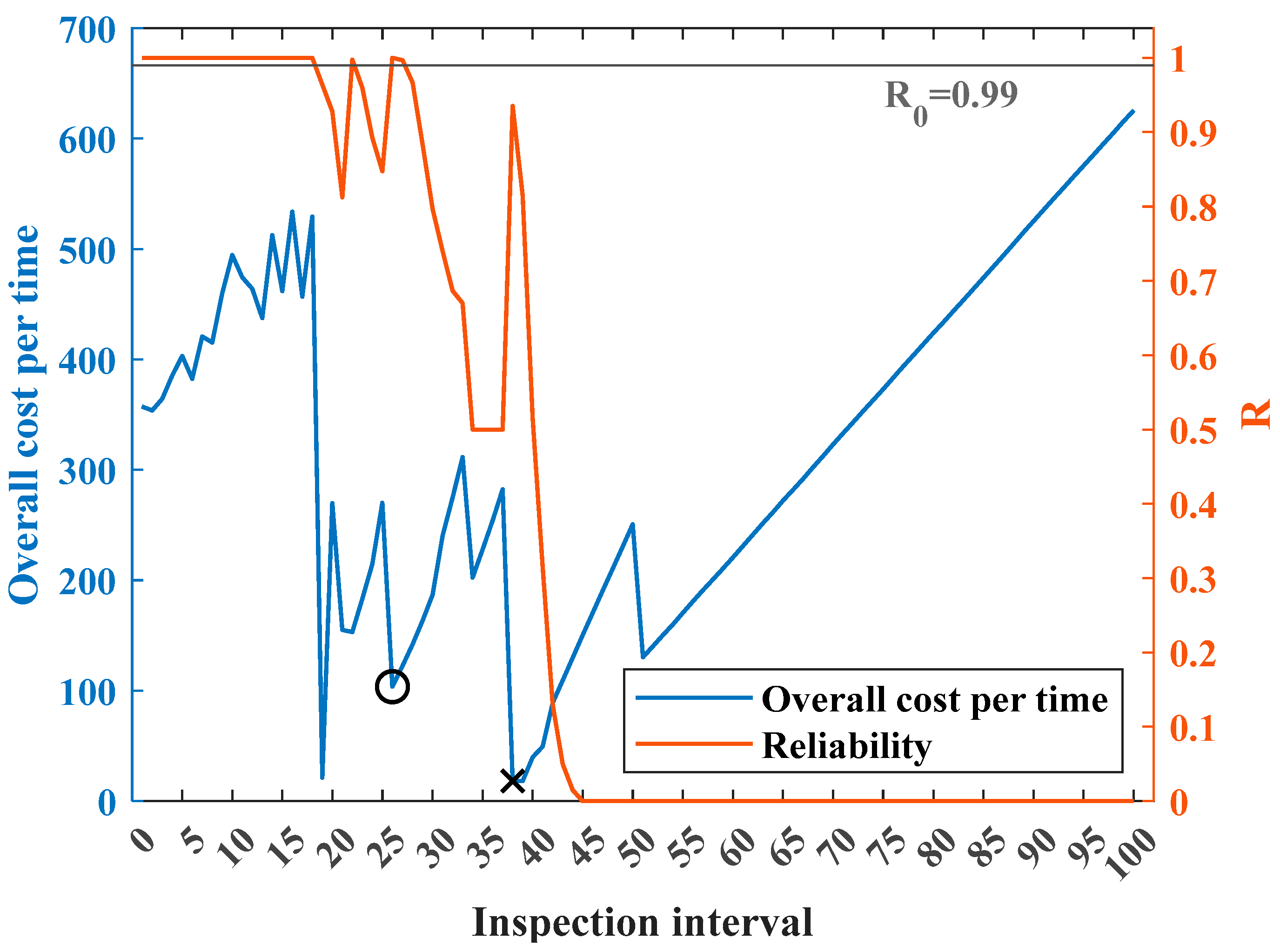
5.1. Optimal Results

For a product-making maintenance decision based on condition monitoring, parameters are provided in Table 1.
We simulate the model on MATLAB for 10,000 times; the optimal inspection interval is 26 h; the minimal overall cost per time is 103.4813 K/h.

5.2. Analysis of the Optimal Results

As shown in Figure 3, the original degradation of performance margin decreases with the increase in time and soon decreases to below zero. Without any maintenance measure, the performance of this component becomes too poor to continue working. However, with inspections, maintenance, and replacement, restoration of the performance margin occurs. The inspection interval calculated by the proposed optimization model reduces the occurrence of failure and ensures that the value of the performance margin fluctuates in a reasonable range through reliability.
The change in optimal overall cost per time when different inspection intervals are used is shown in Figure 4. The total cost of preventive maintenance and the loss in unplanned downtime after failure are two main factors that influence the optimal overall cost per time. When inspection intervals are short, frequent preventive maintenance is required; failure rarely happens. Therefore, the cost of preventive maintenance is greater than the loss after failure. Additionally, when inspection intervals are long, the poor state of the performance margin cannot be detected in time, which sometimes leads to failure. In such situations, the total cost of replacement after failure is created. Limited by fewer inspections, the replacement will not be made often, and the total cost of replacement after failure is not significant. If the failed component is left for a long time, the loss in unplanned downtime after failure increases rapidly and its influence on overall cost is soon greater than the cost of preventive maintenance.
It is also noteworthy that the loss in unplanned downtime after failure increases linearly when the inspection interval is over 50 h. This is caused by the following reasons. Firstly, according to Equation (1) and the parameters in Table 1 (which also can be seen in Figure 3), the failure will occur at around 40 h if there has been no prior maintenance or replacement. Then, since the failure occurs before 50 h, the performance margin is below zero after 50 h. According to Equation (18), there is a linear relationship between the loss in unplanned downtime after failure and the performance margin. The later the failure is inspected and found, the more the performance margin deviates from zero and the higher the loss is. And this leads to a linear relationship between the loss in unplanned downtime after failure and the inspection interval. Finally, when the inspection interval is more than 50 h, there is only one inspection to be taken. After the maintenance and replacement following this inspection, the performance margin will not be updated again; the linear relationship between the loss in unplanned downtime after failure and the inspection interval will not be changed. Thus, the loss in unplanned downtime after failure increases linearly.
During the maintenance measure decision procedure, the expected value of the performance margin is fixed. It guides us to make maintenance decisions based on the fixed expected value, and the impact of dispersion and inconsistency on performance margin is ignored. If the performance margin is very close to (but does not exceed) the maintenance measure threshold, no maintenance measures will be taken. However, if there is a little deviation of the performance margin, the actual value of it can fluctuate below the threshold. It can result in no measure to be taken when failure occurs. This strategy puts decision-makers at risk, so as a result, we introduce reliability obtained by the performance margin (not the expected value) as a constraint.
The influence of reliability on optimal results is showed in Figure 5; the ‘x’ point is the optimal result without the reliability constraint and the ‘o’ point is the optimal result with the reliability constraint. With the constraint of reliability, the optimal inspection interval is shortened, and the minimal overall cost per time increases. This suggests that the reliability constraint is effective, so that we can control the risk while optimizing the cost.
These performances are consistent with the assumed maintenance strategy, and therefore, optimal inspection intervals can be obtained when minimizing the overall cost per time.

5.3. Effect of the Parameters

To investigate the effect of the parameters in the proposed model on optimal solution and maintenance strategy, we vary each of the parameter values and obtain the corresponding inspection intervals T and overall cost per time C ¯ .

5.3.1. Effect of Parameters in Wiener Process

Table 2 summarizes the results of several alternative values for λ . As λ increases, the optimal inspection interval decreases, and the overall cost per time changes accordingly. This simply shows that the faster the performance margin degrades, the sooner it reaches failure, and the earlier the loss in unplanned downtime becomes the main factor that influences the overall cost per time.

5.3.2. Effect of Parameters for Performance Margin

Table 3 presents the corresponding results of different values for m 0 . As m 0 increases, the inspection intervals increase, as well. This demonstrates that the more the performance margin is set aside at the beginning, the later a component can be inspected, and the less overall cost will be incurred.
Table 4 presents the corresponding results of different values for m P d M and m P d R . As m P d M and m P d R increase, the optimal results show no obvious regular pattern. There is a problem to be pointed out here. Whether to take the maintenance measures or not depends on the performance margin at inspections and the maintenance measure threshold vector. However, the cost of several preventive maintenance procedures is more than the cost of a few preventive replacements. Although the cost of a single replacement is more than the cost of a single maintenance procedure, we can still find out that the optimal result is obtained when just a few preventive maintenance procedures but no preventive replacement is taken.

5.3.3. Effect of Parameters Related to Cost

Table 5 summarizes the optimal inspection intervals and cost for several values of c P T and c R P . As c P T and c R P increase, the optimal T decreases first and then basically remains unchanged. The optimal results of C ¯ generally increase because the total cost, including c P T and c R P , also increases.
Table 6 and Table 7 shows that the optimal results for different c P d M , k P d M , C , c D T , C D T 0 and k t h , C values are all generally unchanged. That is because the optimal result is obtained when just a few times of preventive maintenance but no preventive replacement are performed, and these parameters are not related to replacement.

6. Conclusions

In this paper, we provide a condition-based maintenance optimization method using performance margin. A maintenance-involved degradation model of performance margin is developed and assumed to be expressed by a multi-stage Wiener process. We introduce a maintenance measure effect factor to better describe the restoration effect of performance margin after three kinds of maintenance measures. We use maintenance measure decision vectors and maintenance measure threshold vectors to make maintenance decisions and build relationships between the value of the performance margin before and after the maintenance measures. An optimization model of the maintenance decision problem is developed based on the degradation model we developed. Additionally, the reliability constraint based on the performance margin is proposed. The numerical example shows that the results calculated by the proposed model are consistent with the assumed maintenance strategy and improves the maintenance decision process.
However, there are still some imperfections. The proposed maintenance-involved degradation model only considers the working time of products, and neglects the time of inspection, preventive maintenance, preventive replacement, halt after failure, replacement after failure, etc. Additionally, the effect of maintenance only reflects the extent to which the performance margin can revert. However, in practice, maintenance can also influence the degradation trend, that is, the drift parameter, λ , can be changed by maintenance. To build a more practical optimization model, these matters need further studies. For example, the durations of replacement and maintenance can be introduced in the proposed model, and the maintenance effect factor can act on the degradation rate. Also, further research on the methods for determining the value of the maintenance effect factor is necessary. One possible direction is to collect the data for the maintenance effect, and the maintenance effect factor can be obtained by parameter estimation. Another feasible method is to apply expert evaluation for different preventive maintenance actions to subjectively evaluate the maintenance effect factor. Finally, a maintenance optimization model based on the performance margin for the multi-component system can be further studied.

Author Contributions

Conceptualization, S.L. and M.W.; methodology, S.L.; software, S.L.; validation, S.L., M.W., and T.Z.; formal analysis, S.L., M.W., and T.Z.; investigation, S.L.; resources, M.W. and R.K.; data curation, S.L.; writing—original draft preparation, S.L. and T.Z.; writing—review and editing, S.L. and T.Z.; visualization, S.L.; supervision, M.W. and R.K.; project administration, M.W. and R.K.; funding acquisition, T.Z. and R.K. All authors have read and agreed to the published version of the manuscript.

Funding

This research was funded by National Natural Science Foundation of China, grant number 72201013 and 62073009.

Data Availability Statement

The all data presented in the article does not require copyright. They are freely available from the authors.

Conflicts of Interest

The authors declare no conflict of interest.

References

  1. Khan, S.A.; Islam, T.; Khera, N.; Agarwala, A.K. On-line condition monitoring and maintenance of power electronic converters. J. Electron. Test.-Theory Appl. 2014, 30, 701–709. [Google Scholar] [CrossRef]
  2. Munoz-Condes, P.; Gomez-Parra, M.; Sancho, C.; San Andres, M.A.G.; Gonzalez-Fernandez, F.J.; Carpio, J.; Guirado, R. On condition maintenance based on the impedance measurement for traction batteries: Development and industrial implementation. IEEE Trans. Ind. Electron. 2013, 60, 2750–2759. [Google Scholar] [CrossRef]
  3. Kumar, S.; Goyal, D.; Dang, R.K.; Dhami, S.S.; Pabla, B.S. Condition based maintenance of bearings and gears for fault detection—A review. Mater. Today Proc. 2018, 5, 6128–6137. [Google Scholar] [CrossRef]
  4. Giorgio, M.; Guida, M.; Pulcini, G. A state-dependent wear model with an application to marine engine cylinder liners. Technometrics 2010, 52, 172–187. [Google Scholar] [CrossRef]
  5. Kang, J.C.; Wang, Z.H.; Soares, C.G. Condition-based maintenance for offshore wind turbines based on support vector machine. Energies 2020, 13, 17. [Google Scholar] [CrossRef]
  6. Merigand, A.; Ringwood, J.V. Condition-based maintenance methods for marine renewable energy. Renew. Sust. Energ. Rev. 2016, 66, 53–78. [Google Scholar] [CrossRef]
  7. Zhong, Z.Q.; Xu, L.; Xu, J.P. ISHM-oriented time decision-making for condition-based maintenance of multistate systems. IEEE Trans. Aerosp. Electron. Syst. 2020, 56, 15–29. [Google Scholar] [CrossRef]
  8. Ayo-Imoru, R.M.; Cilliers, A.C. A survey of the state of condition-based maintenance (CBM) in the nuclear power industry. Ann. Nucl. Energy 2018, 112, 177–188. [Google Scholar] [CrossRef]
  9. Garramiola, F.; Poza, J.; Madina, P.; del Olmo, J.; Almandoz, G. A review in fault diagnosis and health assessment for railway traction drives. Appl. Sci.-Basel 2018, 8, 19. [Google Scholar] [CrossRef]
  10. Lewandowski, M.; Scholz-Reiter, B. A framework for systematic design and operation of condition-based maintenance systems: Application at a german sea port. Int. J. Ind. Eng.-Theory Appl. Pract. 2013, 20, 2–11. [Google Scholar]
  11. Cha, J.H.; Finkelstein, M. Optimal long-run imperfect maintenance with asymptotic virtual age. IEEE Trans. Reliab. 2016, 65, 187–196. [Google Scholar] [CrossRef]
  12. Ben Mabrouk, A.; Chelbi, A.; Radhoui, M. Optimal imperfect maintenance strategy for leased equipment. Int. J. Prod. Econ. 2016, 178, 57–64. [Google Scholar] [CrossRef]
  13. Yan, B.; Zhou, Y.F.; Liu, L.B. Condition based maintenance of the yaw motor in a wind turbine using an indirect indicator: A case study. In Proceedings of the 2018 Prognostics and System Health Management Conference, New York, NY, USA, 26–28 October 2018; pp. 860–865. [Google Scholar]
  14. Sikorska, J.Z.; Hodkiewicz, M.; Ma, L. Prognostic modelling options for remaining useful life estimation by industry. Mech. Syst. Signal Process. 2011, 25, 1803–1836. [Google Scholar] [CrossRef]
  15. Tai, A.H.; Chan, L.-Y.; Zhou, Y.; Liao, H.; Elsayed, E.A. Condition based maintenance of periodically inspected systems. In Proceedings of the World Congress on Engineering 2009, London, UK, 1–3 July 2009; Volume I–II, p. 1256–+. [Google Scholar]
  16. Besnard, F.; Bertling, L. An Approach for Condition-Based Maintenance Optimization Applied to Wind Turbine Blades. IEEE Trans. Sustain. Energy 2010, 1, 77–83. [Google Scholar] [CrossRef]
  17. Nguyen, K.T.P.; Phuc, D.; Khac Tuan, H.; Berenguer, C.; Grall, A. Joint optimization of monitoring quality and replacement decisions in condition-based maintenance. Reliab. Eng. Syst. Saf. 2019, 189, 177–195. [Google Scholar] [CrossRef]
  18. Dong, Y.L.; Gu, Y.J.; Yang, K. Research on the condition based maintenance decision of equipment in power plant. In Proceedings of the 2004 International Conference on Machine Learning and Cybernetics, New York, NY, USA, 26–29 August 2004; Volume 1–7, pp. 3468–3473. [Google Scholar]
  19. Jardine, A.K.S.; Lin, D.; Banjevic, D. A review on machinery diagnostics and prognostics implementing condition-based maintenance. Mech. Syst. Signal Process. 2006, 20, 1483–1510. [Google Scholar] [CrossRef]
  20. Li, X.-Y.; Chen, W.-B.; Kang, R. Performance margin-based reliability analysis for aircraft lock mechanism considering multi-source uncertainties and wear. Reliab. Eng. Syst. Saf. 2021, 205, 107234. [Google Scholar] [CrossRef]
  21. Li, Y.; Tong, B.-A.; Chen, W.-B.; Li, X.-Y.; Zhang, J.-B.; Wang, G.-X.; Zeng, T. Performance Margin Modeling and Reliability Analysis for Harmonic Reducer Considering Multi-Source Uncertainties and Wear. IEEE Access 2020, 8, 171021–171033. [Google Scholar] [CrossRef]
  22. Nikulin, M.S.; Limnios, N.; Balakrishnan, N.; Kahle, W.; Huber-Carol, C. Advances in Degradation Modeling: Applications to Reliability, Survival Analysis, and Finance; Birkhäuser: Boston, MA, USA, 2010; p. XXXVIII, 416. [Google Scholar]
Figure 1. Framework of the proposed condition-based maintenance optimization method using performance margin.
Axioms 12 00168 g001
Figure 2. Illustration of the maintenance-involved degradation process.
Axioms 12 00168 g002
Figure 3. Optimal maintenance process when inspection intervals are 25, 26 and 27.
Axioms 12 00168 g003
Figure 4. The overall cost per time when different inspection intervals are used.
Axioms 12 00168 g004
Figure 5. The reliability and overall cost per time when different inspection intervals are used.
Axioms 12 00168 g005
Table 1. Parameters in the numerical example.
ParametersValue
λ 5 (mm/hours)
σ 1
m 0 200 (mm)
m P d M 100 (mm)
m P d R 20 (mm)
N 100
c P T ¥100 (K)
c P d M ¥300 (K)
k P d M , C ¥100 (K)
c R P ¥800 (K)
c D T ¥1000 (K)
C D T o ¥2000 (K)
k t h , C 5
p 0.5
R 0 0.99
Table 2. Optimal results for several alterative values for λ .
Value T C ¯
λ = 2511.0101
λ = 526103.4813
λ = 101945.4545
λ = 205543.4563
λ = 502648.9282
Table 3. Optimal results for different values of m 0 .
Value T C ¯
m 0 = 1202136.3636
m 0 = 15027198.1986
m 0 = 20026103.4813
m 0 = 300589.0909
m 0 = 400511.0101
Table 4. Optimal results for different m P d M and m P d R .
Value T C ¯ Value T C ¯
m P d M = 253718.1818 m P d R = 52351.7344
m P d M = 30658.4820 m P d R = 102352.5123
m P d M = 503718.1818 m P d R = 2026103.4813
m P d M = 10026103.4813 m P d R = 303518.1818
m P d M = 15037321.2121 m P d R = 403418.1818
m P d M = 18036321.2121 m P d R = 603418.1818
m P d M = 19536321.2121 m P d R = 903418.1818
Table 5. Optimal results for different values of c P T and c R P .
Value T C ¯ Value T C ¯
c P T = 303716.7677 c R P = 35027115.7845
c P T = 5026103.4407 c R P = 6003714.14
c P T = 10026103.4813 c R P = 80026103.4813
c P T = 20027124.5212 c R P = 100026106.7394
c P T = 28027128.1622 c R P = 120027124.9855
Table 6. Optimal results for different values of c P d M and k P d M , C .
Value T C ¯ Value T C ¯
c P d M = 1201921.2121 k P d M , C = 202733.3355
c P d M = 2002784.5315 k P d M , C = 502765.9119
c P d M = 30026103.4813 k P d M , C = 10026103.4813
c P d M = 50026163.4051 k P d M , C = 20026198.7805
c P d M = 70026223.5657 k P d M , C = 50026472.9619
Table 7. Optimal results for different values of c D T , C D T 0 and k t h , C .
Value T C ¯ Value T C ¯ Value T C ¯
c D T = 40026104.5661 C D T 0 = 50027120.1648 k t h , C = 13718.1818
c D T = 6003718.1818 C D T 0 = 100027122.4718 k t h , C = 226103.8442
c D T = 100026103.4813 C D T 0 = 200026103.4813 k t h , C = 526103.4813
c D T = 14003718.1818 C D T 0 = 300026104.7385 k t h , C = 1027122.3621
c D T = 200027122.0350 C D T 0 = 50003718.1818 k t h , C = 2027121.8045
Disclaimer/Publisher’s Note: The statements, opinions and data contained in all publications are solely those of the individual author(s) and contributor(s) and not of MDPI and/or the editor(s). MDPI and/or the editor(s) disclaim responsibility for any injury to people or property resulting from any ideas, methods, instructions or products referred to in the content.

