Complex Dynamics of Rössler–Nikolov–Clodong O Hyperchaotic System: Analysis and Computations

Abstract

This paper discusses the analysis and computations of chaos–hyperchaos (or vice versa) transition in Rössler–Nikolov–Clodong O (RNC-O) hyperchaotic system. Our work is motivated by our previous analysis of hyperchaotic transitional regimes of RNC-O system and the results recently obtained from another researchers. The analysis and numerical simulations show that chaos–hyperchaos transition in RNC-O system is coupled to change in the equilibria type as one large hyperchaotic attractor occurs. Moreover, we show that for this system, a zero-Hopf bifurcation is not possible. We also consider the cases when the divergence of the system is a constant and detected two families of exact solutions.

1. Introduction

Autonomous nonlinear four-dimensional systems of the form

$$\begin{gathered} \frac{dx}{dt}=\dot{x}=f\left(x\right) \mathrm{with} f\left(x\right)=\left(f_1\left(x\right)\hspace{0.17em},\hspace{0.17em}{f}_2\left(x\right)\hspace{0.17em},\hspace{0.17em}{f}_3\left(x\right)\hspace{0.17em},\hspace{0.17em}{f}_4\left(x\right)\right); \\ x=\left(x_1\hspace{0.17em},\hspace{0.17em}{x}_2\hspace{0.17em},\hspace{0.17em}{x}_3\hspace{0.17em},\hspace{0.17em}{x}_4\right) \end{gathered}$$

(1)

can display a rich diversity of periodic, multiple periodic, chaotic and hyperchaotic solutions dependent upon the specific values of one or more bifurcation (control) parameters [1,2,3,4,5]. Such a system is characterized by four Lyapunov exponents ${\lambda }_1\hspace{0.17em},\hspace{0.17em}{\lambda }_2\hspace{0.17em},\hspace{0.17em}{\lambda }_3$ and ${\lambda }_4$. If ${\displaystyle \sum _{i=1}^4{\lambda }_i<0}$, then the system is dissipative and its evolution takes place on an attractor. Now, it is well known that attractors characterized by only one positive Lyapunov exponents are chaotic and they can occur in at least three-dimensional nonlinear systems [5,6,7,8]. On the other hand, for continuous nonlinear four-dimensional dissipative systems, we can observe attractors with two positive Lyapunov exponents [1,9,10]. Historically, from Rössler [11], these systems are for first time named hyperchaotic. For hyperchaotic systems of the form in (1), the possible types of Lyapunov spectra are $\left(+,\hspace{0.17em}+,\hspace{0.17em}0,\hspace{0.17em}-\right)\hspace{0.17em},\hspace{0.17em}\left(+\hspace{0.17em},\hspace{0.17em}0\hspace{0.17em},\hspace{0.17em}0\hspace{0.17em},\hspace{0.17em}-\right)$ and $\left(+\hspace{0.17em},\hspace{0.17em}0\hspace{0.17em},\hspace{0.17em}-\hspace{0.17em},\hspace{0.17em}-\right)$ [1,6,9,11,12].

Recently, a growing interest has been observed in higher-dimensional systems greater than three with chaotic and hyperchaotic behavior [3,7,8,13,14,15,16,17,18,19,20,21,22]. The main reasons are the following: (1) mathematical models of natural phenomena are high dimensional; (2) the possible bifurcations of four-dimensional systems are absent in three-dimensional ones; (3) the characteristic properties (for systems of dimension higher than three) are covering without folds and (4) in high-dimensional systems, a hyperchaotic behavior occurs, which is essentially different from the chaos in low-dimensional models.

Since Meyer et al. [23] and Nikolov [9,24], the transitional processes of hyperchaotic Rössler type systems have been widely considered. Analytical and computational approaches have become increasingly important for nonlinear sciences and are found in more applications in all scientific areas [7,17,22,25,26,27,28]. During the last 10 years, many studies were devoted to the bifurcation scenarios of hyperchaotic systems [13,16,18,19]. This is possible as long as the transition from chaos to hyperchaos (or vice versa) is analytically studied for the case of a small number of parameters (codimension), since in more complex cases, the domain remains widely open.

Recently, in the hyperchaotic Rössler system, main bifurcation scenario leading to a hyperchaos has been demonstrated by Stankevich et al. [13]. The main bifurcation hyperchaotic scenario can be divided into two parts: the first one includes few local and global bifurcations as a homoclinic attractor is created; the second one (which is more complicated) includes cascades of local and global bifurcations as after an external bifurcation, the system becomes hyperchaotic.

Here, we consider the following system:

$$\begin{array}{l}\dot{x}=-y-z\hspace{0.17em},\\ \dot{y}=x+ay+w\hspace{0.17em},\\ \dot{z}=b+b_{1}x+b_{2}y+b_{3}z+b_{4}w+xz\hspace{0.17em},\\ \dot{w}=-cz+dw\hspace{0.17em},\end{array}$$

(2)

where $a=0.25$, $b=3$, $c=0.5$, $d=0.05$ [11], and $b_1,\hspace{0.17em}{b}_2,\hspace{0.17em}{b}_3$ and $b_4$ are real constants. This system was introduced in [2] as a modification of the original Rössler hyperchaotic system named Rössler–Nikolov–Clodong O hyperchaotic system (RNC-O). In the paper comparing the dynamics of the original and the modified system, it was determined that (1) RNC-O only exhibits hyperchaotic behavior when $b_3$ is varied; (2) repeated hyperchaos–chaos–hyperchaos transition can be seen; (3) the hyperchaos is possible for a smaller value of information dimension.

In general, system (2) has two equilibrium (fixed) points $\left({\overline{x}}_{1,2}\hspace{0.17em},\hspace{0.17em}{\overline{y}}_{1,2}\hspace{0.17em},\hspace{0.17em}{\overline{z}}_{1,2}\hspace{0.17em},\hspace{0.17em}{\overline{w}}_{1,2}\right)$, where

$$\begin{array}{l}{\overline{x}}_{1,2}=-\frac{G\pm \sqrt{g+G^2}}{2d}\hspace{0.17em},\hspace{1em}{\overline{y}}_{1,2}=-\frac{G\pm \sqrt{g+G^2}}{2\left(c-ad\right)}\hspace{0.17em},\\ {\overline{z}}_{1,2}=\frac{G\pm \sqrt{g+G^2}}{2\left(c-ad\right)}\hspace{0.17em},\hspace{1em}{\overline{w}}_{1,2}=c\frac{G\pm \sqrt{g+G^2}}{2d\left(c-ad\right)}\hspace{0.17em},\end{array}$$

(3)

and

$$g=4bd\left(c-ad\right)\hspace{0.17em},\hspace{1em}G=b_{4}c-b_1\left(c-ad\right)-d\left(b_2-b_3\right)\hspace{0.17em},$$

(4)

which reduce to a single one if

$$g+G^2=0\hspace{0.17em}.$$

(5)

It is easy to check that in the considered case ($a=0.25$, $b=3$, $c=0.5$, $d=0.05$ [11]) $g+G^2>0$, and hence ${\overline{x}}_{1,2}\hspace{0.17em},\hspace{0.17em}{\overline{y}}_{1,2}\hspace{0.17em},\hspace{0.17em}{\overline{z}}_{1,2}$ and ${\overline{w}}_{1,2}$ are all real numbers. Thus, in this case, there are two different equilibrium points. Note that in Figure A1 (see Appendix A), the values of ${\overline{z}}_{1,2}$ are shown, and those for which the system (2) exhibits hyperchaotic behavior are marked with red color.

In Section 2, we analyze the system (2) in an adiabatic case for its divergence. In Section 3, we investigate equilibria and the coefficient matrix of the linearized system, as we discuss the possible types of transitions to hyperchaos occurring in system (2). In Section 4, numerical examples are presented with some simulation results to illustrate the theoretical results of previous two sections. Finally, we conclude with a summary and some comments in Section 5.

2. Families of Exact Solutions

The divergence of the flow (2) is obtained by

$$D_4=\frac{\partial \dot{x}}{\partial x}+\frac{\partial \dot{y}}{\partial y}+\frac{\partial \dot{z}}{\partial z}+\frac{\partial \dot{w}}{\partial w}=a+d+b_3+x=0.3+b_3+x\hspace{0.17em}.$$

(6)

It can be seen that the RNC-O system has an alternating divergence—see Figure A2 and Figure A3 in Appendix C. The system (2) is dissipative when $D_4<0$, and an attractor exists if we determined the absorbing domain.

Interesting families of exact solutions to systems of form (2), which are not all constants, arise under the assumption that $x=k=const.$ Then, $\dot{x}=0$, $z=-y$, $\dot{z}=-\dot{y}$, and Equation (2) transforms into the following overdetermined system:

$$\dot{y}=k+ay+w\hspace{0.17em},$$

(7)

$$\dot{y}=-b-b_{1}k-\left(b_2-b_3-k\right)y-b_{4}w$$

(8)

$$\dot{w}=cy+dw$$

(9)

Let $b_4\ne -1$ and $k\ne b_2-b_3\pm a$. Then, after subtraction of (7) from (8) and solving for $w$, one obtains

$$w=-\frac{b+\left(b_1+1\right)k}{1+b_4}-\frac{b_2-b_3+a-k}{1+b_4}y$$

(10)

Consequently,

$$\dot{w}=-\frac{b_2-b_3+a-k}{1+b_4}\dot{y}$$

(11)

and the above system (7)–(9) becomes

$$\dot{y}=-\frac{b+\left(b_1-b_4\right)k}{1+b_4}-\frac{b_2-b_3-a{b}_4-k}{1+b_4}y$$

(12)

$$\dot{y}=d\frac{b+\left(b_1+1\right)k}{b_2-b_3+a-k}+\left(d-\frac{\left(1+b_4\right)c}{b_2-b_3+a-k}\right)y$$

(13)

Evidently, Equations (12) and (13) are compatible if and only if

$$d\frac{b+\left(b_1+1\right)k}{b_2-b_3+a-k}=-\frac{b+\left(b_1-b_4\right)k}{1+b_4}$$

(14)

and

$$d-\frac{\left(1+b_4\right)c}{b_2-b_3+a-k}=-\frac{b_2-b_3-a{b}_4-k}{1+b_4}$$

(15)

Now, it is easy to see that

$$\begin{array}{l}x=k\hspace{0.17em},\\ y=-\frac{b+\left(b_1-b_4\right)k}{b_2-b_3-a{b}_4-k}+c_1{e}^{-\frac{b_2-b_3-a{b}_4-k}{1+b_4}t},\\ z=\frac{b+\left(b_1-b_4\right)k}{b_2-b_3-a{b}_4-k}-c_1{e}^{-\frac{b_2-b_3-a{b}_4-k}{1+b_4}t},\\ w=\frac{a\left(b+b_{1}k\right)-\left(b_2-b_3-k\right)k}{b_2-b_3-a{b}_4-k}-c_1\frac{b_2-b_3+a-k}{1+b_4}{e}^{-\frac{b_2-b_3-a{b}_4-k}{1+b_4}t},\end{array}$$

(16)

where $c_1$ is an arbitrary constant, is a one-parameter family of solutions of system (2), provided that the compatibility conditions (14) and (15) hold.

Next, let $b_4=-1$. Then, subtracting Equation (8) from Equation (7), we obtain

$$b+\left(b_1+1\right)k+\left(b_2-b_3+a-k\right)y=0$$

(17)

Hence, $b+\left(b_1+1\right)k=0$ and $b_2-b_3+a-k=0$ are the necessary and sufficient conditions for the compatibility of the aforementioned two equations. Suppose now that

$$k=b_2-b_3+a\hspace{0.17em},\hspace{1em}{b}_1=-1-\frac{b}{b_2-b_3+a}$$

(18)

Then, solving Equation (7) for $w$ and taking into account the above relations, we obtain

$$w=\dot{y}-ay-a-b_2+b_3$$

(19)

and

$$\dot{w}=\ddot{y}-a\dot{y}$$

(20)

Substituting (19) and (20) into (9), we obtain the following equation:

$$\ddot{y}-\left(a+d\right)\dot{y}+\left(c+ad\right)y+\left(b_2-b_3+a\right)d=0$$

(21)

whose general solution is

$$y=A_0+c_2{e}^{At}+c_3{e}^{Bt}$$

(22)

where $c_2$ and $c_3$ are arbitrary constants, and

$$A_0=-\frac{b_2-b_3+a}{c+ad}d$$

(23)

$$A=\frac{1}{2}\left(a+d-\sqrt{{\left(a-d\right)}^2-4c}\right)\hspace{0.17em},\hspace{1em}B=\frac{1}{2}\left(a+d+\sqrt{{\left(a-d\right)}^2-4c}\right)$$

(24)

Finally, using (19) and (22), we obtain the following two-parameter family of solutions of system (2):

$$\begin{array}{l}x=k\hspace{0.17em}=b_2-b_3+a\hspace{0.17em},\\ y=A_0+c_2{e}^{At}+c_3{e}^{Bt}\hspace{0.17em},\\ z=-A_0-c_2{e}^{At}-c_3{e}^{Bt}\hspace{0.17em},\\ w=-a\left(1+A_0\right)-b_2+b_3+c_2\left(A-a\right)e^{At}+c_3\left(B-a\right)e^{Bt}.\end{array}$$

(25)

Some exact solutions of (2) are shown in Figure A4, Figure A5 and Figure A6 (see Appendix D).

3. Qualitative Behavior for System (2) in Dissipative Case

3.1. Local Analysis

It easy to express (2) in terms of local coordinates $x_1,\hspace{0.17em}{x}_2,\hspace{0.17em}{x}_3$ and $x_4$, where $\overline{x},\hspace{0.17em}\overline{y},\hspace{0.17em}\overline{z}$ and $\overline{w}$ were defined in (3)

$$x=\overline{x}+x_1\hspace{0.17em},\hspace{1em}y=\overline{y}+x_2\hspace{0.17em},\hspace{1em}z=\overline{z}+x_3\hspace{0.17em},\hspace{1em}w=\overline{w}+x_4$$

(26)

Hence, after some transformations, we determine that

$$\begin{array}{l}{\dot{x}}_1=-x_2-x_3\hspace{0.17em},\\ {\dot{x}}_2=x_1+a{x}_2+x_4\hspace{0.17em},\\ {\dot{x}}_3=k_1{x}_1+b_2{x}_2+k_2{x}_3+b_4{x}_4+x_1{x}_3\hspace{0.17em},\\ {\dot{x}}_4=-c{x}_3+d{x}_4\hspace{0.17em},\end{array}$$

(27)

where $k_1=b_1+\overline{z}$ and $k_2=b_3+\overline{x}$. The eigenvalues of the Jacobian matrix of system (6) (for the equilibria (3)) can be computed through the determinant

$$\mathsf{\Xi }\left(\chi \right)=\left|\begin{array}{l}-\chi \hspace{1em}\hspace{0.17em}-1\hspace{1em}\hspace{0.17em}\hspace{0.17em}-1\hspace{1em}\hspace{1em}0\\ \hspace{0.17em}\hspace{0.17em}\hspace{0.17em}1\hspace{1em}\hspace{0.17em}a-\chi \hspace{1em}\hspace{0.17em}\hspace{0.17em}0\hspace{1em}\hspace{1em}1\\ \hspace{0.17em}\hspace{0.17em}\hspace{0.17em}{k}_1\hspace{1em}\hspace{0.17em}\hspace{0.17em}\hspace{0.17em}{b}_2\hspace{1em}{k}_2-\chi \hspace{1em}{b}_4\\ \hspace{0.17em}\hspace{0.17em}\hspace{0.17em}0\hspace{1em}\hspace{1em}0\hspace{1em}\hspace{0.17em}\hspace{0.17em}-c\hspace{1em}d-\chi \end{array}\right|=0\hspace{0.17em},$$

(28)

which is equivalent to the characteristic equation

$${\chi }^4+p{\chi }^3+q{\chi }^2+r\chi +s=0$$

(29)

where

$$\begin{array}{l}p=-\left(a+d+k_2\right)\hspace{0.17em},\hspace{0.17em}q=1+k_1+a{k}_2+d\left(a+k_2\right)+c{b}_4\hspace{0.17em},\\ r=b_2\left(1+c\right)-k_2\left(1+ad\right)-k_1\left(a+d\right)-d-ac{b}_4\hspace{0.17em},\\ s=k_1\left(ad-c\right)+d\left(k_2-b_2\right)+c{b}_4\hspace{0.17em}\hspace{0.17em}.\end{array}$$

(30)

For n-dimensional dynamic system, according to [9,29,30,31], in principle, six possible equilibrium types (cases) (with even more sub-cases) depending on the roots of the characteristic equation exist. In four-dimensional systems, there are five distinct types (for $t\to +\infty$) at a hyperbolic fixed (equilibrium) point with even more sub-cases. According to [32], they are

$$real\hspace{0.17em}eigenvalue:\hspace{0.17em}\{\begin{array}{l}1)\hspace{0.17em}\hspace{0.17em}{\chi }_{1,2}>0\hspace{0.17em},\hspace{0.17em}{\chi }_{3,4}<0.\hspace{0.17em}\\ 2)\hspace{0.17em}\hspace{0.17em}{\chi }_1>0\hspace{0.17em},\hspace{0.17em}{\chi }_{2,3,4}<0.\end{array}\hspace{1em} \begin{array}{l}{O}^{2,2}\\ O^{3,1}\end{array}$$

$$\begin{array}{l}complex\hspace{0.17em}eigenvalues:\hspace{0.17em}3)\hspace{0.17em}{\chi }_{1,2}=n_1\pm i{m}_1\hspace{0.17em},\hspace{0.17em}{\chi }_{3,4}=n_2\pm i{m}_2;\\ \hspace{1em}\hspace{1em}\hspace{1em}\hspace{1em}\hspace{1em}\hspace{1em}\hspace{1em}\hspace{1em}\hspace{1em}\hspace{1em}{n}_1>0\hspace{0.17em},\hspace{0.17em}{n}_2<0\hspace{0.17em},\hspace{0.17em}{m}_1\hspace{0.17em},\hspace{0.17em}{m}_2\ne 0\hspace{0.17em}.\end{array}\hspace{1em} O^{2,2}$$

$$real\hspace{0.17em}and\hspace{0.17em}complex\hspace{0.17em}eigenvalues:|\begin{array}{l}4)\hspace{0.17em}{\chi }_{1,2}=n_1\pm i{m}_1\hspace{0.17em},\hspace{0.17em}{\chi }_{3,4}>0\hspace{0.17em};\hspace{0.17em}{n}_1<0\hspace{0.17em},\hspace{0.17em}{m}_1\ne 0\hspace{0.17em}.\\ 5)\hspace{0.17em}{\chi }_{1,2}=n_1\pm i{m}_1\hspace{0.17em},\hspace{0.17em}{\chi }_3<0\hspace{0.17em},\hspace{0.17em}{\chi }_4>0\hspace{0.17em};\hspace{0.17em}{n}_1<0\hspace{0.17em},\hspace{0.17em}{m}_1\ne 0\hspace{0.17em}.\end{array}\hspace{1em} \begin{array}{l}{O}^{ , 2,2}\\ O^{3,1}\end{array}$$

In all cases when $u+v=n$, $u\ne 0$, and $v\ne 0$, the equilibrium state $O^{u,v}$ is (compound) saddle of first/second order. Moreover, for $t\to -\infty$, we have $O^{2,2}$ and $O^{1,3}$. If $u+v\ne n$, i.e., there are zero(s) root(s), then compound saddle-focus, compound saddle-knot, etc., take place. For more details, see Case 6 in the Appendix of [9]. Note here that if we have purely imaginary roots and roots whose real parts are of different signs, then the equilibrium state is of a complex saddle type (CS).

Figure 1 shows the possible types (cases) for first ($O_1$) and second ($O_2$) equilibria of system (2) depending on the roots of the characteristic Equation (29), when $b_1\in [0.01,\hspace{0.17em}1.5]$, $b_2\in [-2,\hspace{0.17em}-0.01]$, $b_3\in [0.01,\hspace{0.17em}2.5]$, $b_4\in [0.01,\hspace{0.17em}0.7]$ and all another parameters values are as those in original Rössler hyperchaotic system. It can be seen that possible types of $O_1$ and $O_2$ are one and the same. Interestingly, the dominant type of $O_2$ is unstable knot ($O_2^{0,4}$), and the transition between $O_2^{3,1}$ and $O_2^{1,3}$ is not typical, as remarked with dotted line. Note that diagrams in Figure 1 are obtained as a result of direct numerical calculations of (29), not shown here. According to [2,9], transition from chaos to hyperchaos (or vice versa) takes place for system (2) when equilibrium points change its type from compound saddle to compound knot (or vice versa).

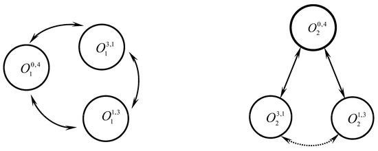
Figure 1. Possible types (cases) and transitions for the first ($O_1$) and the second ($O_2$) equilibria of system (2) depending on the roots of the characteristic Equation (29), when $b_1\in [0.01,\hspace{0.17em}1.5]$, $b_2\in [-2,\hspace{0.17em}-0.01]$, $b_3\in [0.01,\hspace{0.17em}2.5]$, $b_4\in [0.01,\hspace{0.17em}0.7]$ and all another parameter values are as those in the original Rössler hyperchaotic system, see in [11]. The dotted line remarks that transition between $O_2^{3,1}$ and $O_2^{1,3}$ can be seen only in a small number of values for $b_1-b_4$ and that is why it is not typical.

In order to understand mechanisms of the emergence of hyperchaotic attractors, we will analyze the bifurcation of one-parameter families of the model. If a four-dimensional nonlinear system has an isolated equilibrium with double-zero eigenvalue and a pair of purely imaginary eigenvalues (named zero-Hopf equilibrium), then, under certain conditions, some complicated invariant sets could be bifurcated from a zero-Hopf bifurcation [33]. Thus, the zero-Hopf equilibrium, in some cases, can be generator of a local chaos (see [34] and references therein).

Let us come back to the study of the equilibrium points (3) and the characteristic Equation (29). If we assume that $b=c=b_1=b_2=b_3=b_4=0$ into (3), then we always have an equilibrium point for the hyperchaotic system (2) localized at the origin of its coordinates, i.e., we have $E_0\left(0,\hspace{0.17em}0,\hspace{0.17em}0,\hspace{0.17em}0\right)$. In light of this, the following problem arises:

Problem 1.

Is there a one-parameter family of systems of form (2) for which the origin of coordinates (i.e.,$E_0$) is a zero-Hopf equilibrium point?

A general answer to this problem is provided below.

Jacobian matrix (28) evaluated at $E_0$ is

$${\mathsf{\Xi }}_0\left(\chi \right)=\left|\begin{array}{l}-\chi \hspace{1em}\hspace{0.17em}-1\hspace{1em}\hspace{0.17em}\hspace{0.17em}-1\hspace{1em}\hspace{1em}0\\ \hspace{0.17em}\hspace{0.17em}\hspace{0.17em}1\hspace{1em}\hspace{0.17em}a-\chi \hspace{1em}\hspace{0.17em}\hspace{0.17em}0\hspace{1em}\hspace{1em}1\\ \hspace{0.17em}\hspace{0.17em}\hspace{0.17em}0\hspace{1em}\hspace{0.17em}\hspace{0.17em}\hspace{0.17em}\hspace{0.17em}0\hspace{1em}\hspace{0.17em}-\chi \hspace{1em}\hspace{1em}0\\ \hspace{0.17em}\hspace{0.17em}\hspace{0.17em}0\hspace{1em}\hspace{1em}0\hspace{1em}\hspace{0.17em}\hspace{0.17em}\hspace{0.17em}\hspace{0.17em}\hspace{0.17em}0\hspace{1em}d-\chi \end{array}\right|=0\hspace{0.17em},$$

(31)

which is equivalent to the characteristic equation

$${\chi }^4+p_0{\chi }^3+q_0{\chi }^2+r_0\chi +s_0=0$$

(32)

where

$$p_0=-\left(a+d\right)\hspace{0.17em},\hspace{0.17em}{q}_0=1+ad\hspace{0.17em},\hspace{0.17em}{r}_0=-d\hspace{0.17em},\hspace{0.17em}{s}_0=0\hspace{0.17em}.$$

(33)

To satisfy the conditions for $E_0$ to be an isolated equilibrium with double-zero eigenvalue and a pair of purely imaginary eigenvalues, the coefficients $p_0,\hspace{0.17em}{q}_0,\hspace{0.17em}{r}_0$ and $s_0$ must be $p_0=0\hspace{0.17em},\hspace{0.17em}{q}_0<0,\hspace{0.17em}{r}_0=0$ and $s_0=0$, i.e., we must have $a=d=0$. It is easy to see that $q_0=1>0$. Hence, we conclude that the conditions for $E_0$ to be isolated zero-Hopf equilibrium are not valid, and it follows that the zero-Hopf bifurcation for system (2) is not possible. Then, the following theorem can be formulated:

Theorem 1.

If$E_0$is an equilibrium point for the hyperchaotic system (2) localized at the origin of its coordinates, then this equilibrium cannot be of zero-Hopf type. This means that for the system (2), a zero-Hopf bifurcation is not possible.

3.2. Global Behavior

According to [13], the main bifurcation scenarios leading to hyperchaotic behavior can be naturally divided into two parts. The first one includes only a few local and global bifurcations leading to the emergence (in the Poincare map of the system) of a homoclinic attractor—hyperchaotic/chaotic. The second one (which is too complicated) includes (infinite) cascades of local and global bifurcations forming the skeleton of an attractor (with two positive Lyapunov exponents) which becomes hyperchaotic due to an external bifurcation (crisis). As a result, the smaller hyperchaotic attractor is destroyed, as its orbits transfer hyperchaoticity to the larger attractor. In our case, we obtain the same scenario; more precisely, in the second part, the larger attractor (area near $O_1$) starts to become dominant. After the crisis (an external bifurcation for the smaller attractor (area near $O_2$)), the smaller attractor is destroyed and finally disappears. In other words, the two attractors merge into one large hyperchaotic attractor [23]. Note that equilibrium state $O_2$ is mainly a compound unstable knot—$O_2^{0,4}$. This type of behavior is demonstrated in Section 4.

We may summarize the (precise) features described in the second part of the scenario leading to hyperchaos: when the dimension of the system is higher than four (all odd dimensions), then the number of smaller hyperchaotic attractors can be two, three or more, and one of them starts becoming dominant, i.e., the shadowland effect takes place. According to [23], for the generalized Rössler system of dimension $n=7$, two smaller and one large attractor exist. The three attractors, their existence, form and location in phase space are the aftermath of the structural symmetry. In the bifurcation diagram (see Figure 12 in [23]), attractor 1, attractor 2, and attractor 3 (from bottom to top) are in different shadings.

4. Numerical Results

Numerical experiments (results) are very useful for creating basic intuitions and suggesting problems for analytical investigations in chaotic dynamic. It is by far truer in the case of nonlinear systems in $R^4$, which is the subject of our study.

According to [2,9], when Case 1 $b_1=0.1\hspace{0.17em}\hspace{0.17em}or\hspace{0.17em}\hspace{0.17em}1.2$, $b_2=-0.1$, $b_3=b_4=0.1$; Case 2 $b_1=0.2$, $b_2=-0.1$, $b_3=b_4=0.1$; and Case 3 $b_1=b_3=0.2$, $b_2=-0.3$, $b_4=0.01$, the system (2) exhibits hyperchaotic behavior. Here, the numerical computations are used to generate pictures of attractors for system (2) and to determined possible equilibria types. We fix the values of $a,\hspace{0.17em}b,\hspace{0.17em}c$ and $d$ for system (2), and investigate the changes in its behavior with control (bifurcation) parameters $b_1$, $b_2$, $b_3$, and $b_4.$ The solutions for $\left(x\left(t\right),\hspace{0.17em}y\left(t\right),\hspace{0.17em}z\left(t\right),\hspace{0.17em}w\left(t\right)\right)$ have been calculated with initial conditions $x_0=-20,y_0=0,z_0=0,w_0=15$ using MATLAB (the MathWorks, Inc., Natick, MA, USA)- ODE45 solver (which is based on an explicit Runge–Kutta (4,5) formula, the Dormand–Prince pair).

In Figure 2, the phase space (in $\left(x,\hspace{0.17em}y,\hspace{0.17em}z\right)$ and $\left(x,\hspace{0.17em}y,\hspace{0.17em}w\right)$ coordinates) and possible positions of equilibria $O_1$ (red color point) and $O_2$ (blue color point) of system (2) in Case 1 are shown. Here, $O_1$ is compound saddle (i.e., $O_1^{1,3}$ or $O_1^{3,1}$), and $O_2$ can be only compound unstable knot (i.e., $O_2^{0,4}$) for $b_1=0.1$ (see Figure 2a,b), and for $b_1=1.2$ (see Figure 2c,d). Note that eigenvalues are provided in Appendix B. These figures suggest that a larger (dominant) attractor occurs near the location (basin of attraction) of $O_1$. We see that the qualitative results of Section 3 well predict the behavior of system (2) near the chaos-hyperchaos (or vice versa) transitional point. Interestingly, some of the values of $D_4$ (for $b_1=0.1$ or $b_1=1.2$) in Case 1 can be positive and zero; see Figure A2 in Appendix C.

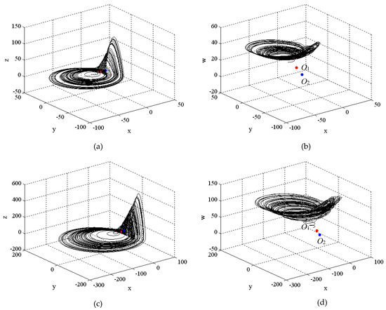
Figure 2. Phase space of system (2) in hyperchaotic regime when (a,b) $a=0.25,\hspace{0.17em}b=3,\hspace{0.17em}c=0.5,\hspace{0.17em}d=0.05,$$b_2=-0.1,\hspace{0.17em}{b}_3=0.1,\hspace{0.17em}{b}_4=0.1$ with $b_1=0.1$; (c,d) $b_1=1.2$. The first equilibrium $O_1$ is marked with red color and the second equilibrium $O_2$ is marked with blue color.

Figure 3 shows the phase spaces of system (2) in Case 2. The equilibrium points $O_1$ and $O_2$ were obtained by using (3). Similar to the results shown in Figure 2, here we see that the motion is also attracted to the first equilibrium point $O_1$ as a larger (dominant) attractor occurs. The result in Figure 3b clearly shows the way in which the smaller hyperchaotic attractor disappears. In this case, $O_1$ is compound saddle (i.e., $O_1^{1,3}$), and $O_2$ is compound unstable knot (i.e., $O_2^{0,4}$); see Appendix B.

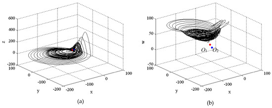
Figure 3. Phase space of system (2) in hyperchaotic regime, when (a,b) $a=0.25,\hspace{0.17em}b=3,\hspace{0.17em}c=0.5,\hspace{0.17em}d=0.05,$$b_1=0.2,\hspace{0.17em}{b}_2=0.1,\hspace{0.17em}{b}_3=b_4=0.1$. The first equilibrium $O_1$ is marked with red color and the second equilibrium $O_2$ is marked with blue color.

Finally, we investigate Case 3 when $b_1=b_3=0.2$, $b_2=-0.3$, $b_4=0.01$. Figure 4 shows the phase spaces of system (2). As can be seen, similar to the previous Figure 2 and Figure 3, the motion is attracted to the first equilibrium point $O_1$, which is compound saddle (i.e., $O_1^{3,1}$). Here, $O_2$ is also compound unstable knot (i.e., $O_2^{0,4}$); see Appendix B.

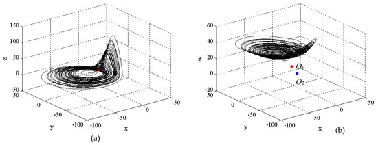
Figure 4. Phase space of system (2) in hyperchaotic regime, when (a,b) $a=0.25\hspace{0.17em},\hspace{0.17em}b=3\hspace{0.17em},\hspace{0.17em}c=0.5\hspace{0.17em},\hspace{0.17em}d=0.05\hspace{0.17em},\hspace{0.17em}{b}_1=0.2\hspace{0.17em},\hspace{0.17em}{b}_2=-0.3\hspace{0.17em},\hspace{0.17em}{b}_3=0.2,b_4=0.01$. The first equilibrium $O_1$ is marked with red color and the second equilibrium $O_2$ is marked with blue color.

Comparing Figure 2, Figure 3 and Figure 4, we conclude that our hypothesis appears to be realistic; that is, the hyperchaotic behavior of the system (2) depends on the type of equilibria—compound saddle and compound knot. As a result, a larger (dominant) attractor occurs near the location (basin) of $O_1$. Note that this conclusion is in accordance with the scenario described in Section 3.2.

5. Conclusions

The present paper provides some new results and can be seen in part as an extension of earlier works on the RNC-O system (2) in [2,9]. Our main motivation comes from previous theoretical [13,16] and numerical works [9,24] which showed that specific cascades of local and global bifurcations might occur.

According to [35,36], for systems with an alternating divergence, the existence of new very unexpected and interesting dynamical regimes can be seen. To understand the effect of this alternating divergence on the dynamical organization of RNC-O system, in Section 2, we obtain two families of exact solutions of systems (2) under the assumption that its divergence is a constant, i.e., $x=k=const$.

As mentioned in Section 3, our goal was to study the equilibria type changes associated to a chaos–hyperchaos transition problem in RNC-O system. Thus, we determine that when equilibrium points change its type from compound saddle to compound knot (or vice versa), the hyperchaos occurs. Moreover, in Section 3.2, we precise the Stankevich’s scenario for hyperchaos transition [13] when one system displays a number of dimensions higher than four, i.e., the so-called shadowland effect takes place. Finally, in Section 3.1, we demonstrate that for RNC-O system, a zero-Hopf bifurcation is not possible. Hyperchaos behavior raises a number of further questions that we leave to future research.

References

- Letellier, C.; Rossler, O.E. Hyperchaos. Scholarpedia 2007, 2, 1936. [Google Scholar] [CrossRef]
- Nikolov, S.; Clodong, S. Occurrence of regular, chaotic and hyperchaotic behavior in a family of modified Rossler hyperchaotic systems. Chaos Solitons Fractals 2004, 22, 407–431. [Google Scholar] [CrossRef]
- Nikolov, S. Estimating of bifurcations and chaotic behavior in a four-dimensional system. J. Calcutta Math. Soc. 2006, 2, 17–28. [Google Scholar]
- Panchev, S. Theory of Chaos; Bulgarian Acad. Press: Sofia, Bulgaria, 2001. [Google Scholar]
- Peng, J.; Ding, E.; Ding, M.; Yang, W. Synchronizing hyperchaos with a scalar transmitted signal. Phys. Rev. Lett. 1996, 76, 904. [Google Scholar] [CrossRef] [PubMed]
- Wolf, A.; Swift, J.; Swinney, H.; Vastano, J. Determining Lyapunov exponents from a time series. Phys. D Nonlinear Phenom. 1985, 16, 285–317. [Google Scholar] [CrossRef]
- Jahanshahi, H.; Yousefpour, A.; Wei, Z.; Alcaraz, R.; Bekiros, S. A financial hyperchaotic system with coexisting attractors: Dynamic investigation, entropy analysis, control and synchronization. Chaos Solitons Fractals 2019, 126, 66–77. [Google Scholar] [CrossRef]
- Pavlov, A.; Pavlova, O.; Mohammad, Y.; Kurths, J. Characterization of the chaos-hyperchaos transition based on return times. Phys. Rev. E 2015, 91, 022921. [Google Scholar] [CrossRef]
- Nikolov, S.; Clodong, S. Hyperchaos-chaos-hyperchaos transition in modified Rossler type systems. Chaos Solitons Fractals 2006, 28, 252–263. [Google Scholar] [CrossRef]
- Alligood, K.; Sauer, T.; Yorke, J. Chaos, An Introduction to Dynamical System; Springer: New York, NY, USA, 1996. [Google Scholar]
- Rössler, O. An equation for hypechaos. Phys. Lett. A 1979, 71A, 155–157. [Google Scholar] [CrossRef]
- Wang, X.; Wang, M. A hyperchaos generalized from Lorenz system. Phys. A Stat. Mech. Its Appl. 2008, 387, 3751–3758. [Google Scholar] [CrossRef]
- Stankevich, N.; Kazakov, A.; Gonchenko, S. Scenarios of hyperchaos occurence in 4D Rössler system. Chaos Interdiscip. J. Nonlinear Sci. 2020, 30, 123129. [Google Scholar] [CrossRef]
- Starkov, K. On the ultimate dynamics of the four-dimensional Rössler system. Int. J. Bifurc. Chaos 2014, 24, 1450149. [Google Scholar] [CrossRef]
- Szczepaniak, A.; Macek, W. Unstable manifolds for the hyperchaotic Rossler system. Phys. Lett. A 2008, 372, 2423–2427. [Google Scholar] [CrossRef]
- Barrio, R.; Martinez, M.; Serrano, S.; Wilczak, D. When chaos meets hyperchaos: 4D Rossler model. Phys. Lett. A 2015, 379, 2300–2305. [Google Scholar] [CrossRef]
- Kuptsov, P.; Kuznetsov, S. Route to hyperbolic hyperchaos in a nonautonomous time-delay system. Chaos Interdiscip. J. Nonlinear Sci. 2020, 30, 113113. [Google Scholar] [CrossRef] [PubMed]
- Stankevich, N.; Volkov, E. Chaos–hyperchaos transition in three identical quorum-sensing mean-field coupled ring oscillators. Chaos Interdiscip. J. Nonlinear Sci. 2021, 31, 103112. [Google Scholar] [CrossRef] [PubMed]
- Sataev, I.; Stankevich, N. Cascade of torus birth bifurcations and inverse cascade of Shilnikov attractors merging at the threshold of hyperchaos. Chaos Interdiscip. J. Nonlinear Sci. 2021, 31, 023140. [Google Scholar] [CrossRef]
- Li, Q.; Tang, S.; Yang, X. Hyperchaotic set in continuous chaos–hyperchaos transition. Commun. Nonlinear Sci. Numer. Simul. 2014, 19, 3718–3734. [Google Scholar] [CrossRef]
- Karatetskaia, E.; Shykhmamedov, A.; Kazakov, A. Shilnikov attractors in three-dimensional orientation-reversing maps. Chaos Interdiscip. J. Nonlinear Sci. 2021, 31, 011102. [Google Scholar] [CrossRef]
- Lai, Q.; Norouzi, B.; Liu, F. Dynamic analysis, circuit realization, control desing and image encryption application of an extended Lü system with coexisting attractors. Chaos Solitons Fractals 2018, 114, 230–245. [Google Scholar] [CrossRef]
- Meyer, T.; Bünner, M.; Kittel, A.; Parisi, J. Hyperchaos in the generalized Rössler system. Phys. Rev. E 1997, 56, 5069–5082. [Google Scholar] [CrossRef]
- Nikolov, S. Transitional processes in some modified Rossler type dynamical systems. Comptes Rendus L’academie Bulg. Sci. 2004, 57, 45–52. [Google Scholar]
- Schuster, H. Deterministic Chaos: An introduction; Physik-Verlag: Berlin, Germany, 1984. [Google Scholar]
- Kapitaniak, T.; Maistrenko, Y.; Popovych, S. Chaos-hyperchaos transition. Phys. Rev. E 2000, 62, 1972–1976. [Google Scholar] [CrossRef] [PubMed]
- Hirsch, M.; Smale, S.; Devaney, R. Differential Equations, Dynamical Systems, and An Introduction to Chaos; Academic Press: New York, NY, USA, 2012. [Google Scholar]
- Singh, S.; Han, S.; Lee, S.M. Adaptive single input sliding mode control for hybrid-synchronization of uncertain hyperchaotic Lu systems. J. Frankl. Inst. 2021, 358, 7468–7484. [Google Scholar] [CrossRef]
- Nemytskii, V.; Stepanov, V. Qualitative Theory of Differential Equations; Princeton University Press: Princeton, NJ, USA, 1960. [Google Scholar]
- Mints, R. The character of certain types of complex equilibrium state in n-dimensional spaces. DAN USSR 1962, 147, 31–33. [Google Scholar]
- Gavrilov, N. On n-dimensional dynamic systems close to the systems with non-rough homoclinic curve. DAN USSR 1973, 212, 276–279. [Google Scholar]
- Wiggins, S. Global Bifurcations and Chaos: Analytical Methods; Springer: New York, NY, USA, 1988. [Google Scholar]
- Cid-Montiel, L.; Llibre, J.; Stoica, C. Zero-Hopf bifurcation in a hyperchaotic Lorenz system. Nonlinear Dyn. 2014, 75, 561–566. [Google Scholar] [CrossRef]
- Champney, A.; Kirk, V. The entwined wiggling of homoclinic curves emerging from saddle-node/Hopf instabilities. Phys. D Nonlinear Phenom. 2004, 195, 77–105. [Google Scholar] [CrossRef]
- Gonchenko, S.; Turaev, D. On three types of dynamics and notation of attractor. Proc. Steklov Inst. Math. 2017, 297, 116–137. [Google Scholar] [CrossRef]
- Gonchenko, S.; Gonchenko, A.; Kozlov, A. Three types of attractors and mixed dynamics of nonholonomic models of rigid body motion. Proc. Steklov Inst. Math. 2020, 308, 125–140. [Google Scholar] [CrossRef]
Disclaimer/Publisher’s Note: The statements, opinions and data contained in all publications are solely those of the individual author(s) and contributor(s) and not of MDPI and/or the editor(s). MDPI and/or the editor(s) disclaim responsibility for any injury to people or property resulting from any ideas, methods, instructions or products referred to in the content. |
© 2023 by the authors. Licensee MDPI, Basel, Switzerland. This article is an open access article distributed under the terms and conditions of the Creative Commons Attribution (CC BY) license (https://creativecommons.org/licenses/by/4.0/).