Article

Improved Cascade Correlation Neural Network Model Based on Group Intelligence Optimization Algorithm

1
School of Computer Science and Technology, Dongguan University of Technology, Dongguan 523808, China
2
School of Computer and Information, Dongguan City College, Dongguan 523419, China
*
Author to whom correspondence should be addressed.
Axioms 2023, 12(2), 164; https://doi.org/10.3390/axioms12020164
Submission received: 6 December 2022 / Revised: 28 January 2023 / Accepted: 31 January 2023 / Published: 6 February 2023
(This article belongs to the Special Issue Fractional-Order Equations and Optimization Models in Engineering)

Abstract

:
The Cascade Correlation learning algorithm is a special supervised learning algorithm for artificial neural network architecture. The optimization algorithm in the traditional neural network has the disadvantages of a single optimization goal, slow convergence speed, and can easily fall into local area, which cannot fully meet the key elements in the cascade correlation learning algorithm. In comparison, the group intelligence optimization algorithm can take into account these key elements in the optimization process at the same time, and obtain better optimization results. In this paper, we propose the single-objective optimization algorithm jDE-B and the multi-objective optimization algorithm MOEA-T, and improve the network expansion mode in the learning process of Cascade Correlation neural networks. We investigate the effect of applying the group intelligent optimization algorithm in the Cascade Correlation learning algorithm. Experimental results show that our improved algorithm is able to enhance the ability of the Cascade Correlation neural network to fit problems, reduce the number of hidden units and the depth of the network, and optimize the network structure.

1. Introduction

With the development of neural networks, the design structure of neural networks is becoming more and more complex. According to the different adaptive algorithms [1] proposed by the researchers for neural network structure optimization, they can be divided into three categories: constructive algorithm [2,3,4,5], pruning algorithm [6,7,8] and hybrid algorithm [9,10,11]. The Cascade Correlation neural network (CCNN) is a new artificial neural network architecture and supervised learning algorithm that was proposed by Scott E. Fahlman and Christian Lebiere in 1991 [12]. It can be classified as one of the constructive algorithms. The Cascade Correlation learning algorithm starts with a minimal network, then trains one by one and adds new hidden units to create a multi-layer structured neural network. Once a trained hidden unit is fixed to the network, its input weights are frozen. Then the network continues to train and add hidden units. Compared with existing algorithms, the cascade correlation architecture has several advantages: (1) It learns quickly, and the network determines its own size and topology. (2) Even when the training set changes, it retains the constructed structure and does not need to back propagate the error signal through the network [13].
Many different types of Cascade Correlation learning algorithms have been developed in the literature [14,15]. There are two key ideas behind the design of the algorithms: The first is the cascaded architecture, the network adds new hidden units one by one. The unit’s input-side weights are frozen. The second is the learning algorithm, which can create and install new hidden units. For each new hidden unit, the Cascade Correlation learning algorithm attempts to maximize the correlation between the output of the new unit and the residual signal of the output unit, which is different from the idea of back-propagation. The major challenge of the Cascade Correlation learning algorithm is how to add appropriate hidden units, which mainly lies in the optimization method of hidden unit weight, the optimization target of the hidden unit, and the selection of the hidden unit’s activation function.
The first problem is that the optimization method of hidden unit weight does not have enough global search capability. In the Cascade Correlation learning algorithm, the current network state will determine the optimization direction of the subsequent network. Therefore, early optimization is very important and will affect the global optimization process. The new hidden unit optimization target is always complex, and the traditional neural network optimization method will often fall into the local area. So the pool of candidate unit strategy is adopted in the Cascade Correlation learning algorithm. There are multiple candidate units in the candidate pool, each with the same link as well as the training target, but with different weights of random initial weights. Each unit did not interact with others during the training, and the candidate unit with the best correlation score was selected as the new hidden unit. Although this mechanism can reduce the probability of adding useless units to the neural network, it is still insufficient. We can try to change the optimization method of the hidden unit weight by using the group intelligent optimization method. The possibility of finding the global optimal solution is relatively high by using the group intelligent optimization method. This is because the number of variables in the early optimization stage of the Cascade Correlation neural network is small. which will add a currently optimal unit to the network [16]. The Cascade Correlation neural network will install the current optimal hidden unit according to the global optimal solution during training.
Group intelligent optimization algorithm is one of the optimization fields which has attracted much attention in recent years. It simulates various group behaviors of social animals and uses the information interaction and cooperation among individuals in the group to achieve the purpose of optimization. Compared with other types of optimization methods, its implementation is relatively simple and more efficient. Group intelligent optimization algorithms mostly do not rely on the gradient information of the optimization function, so they will not have as many problems as the gradient-based optimization algorithm.
In the past, some researchers have tried to use the group intelligence optimization algorithm for the weight optimization of neural networks. In 2011, researcher proposed a new algorithm based on combining a genetic algorithm and a BP neural network, namely the GA-BP algorithm, to solve the defects of poor convergence and partial minima in the BP Neural Network Model. The algorithm will be applied to the initial weights, structure optimization, and learning rule optimization of the BP network. Compared with the simple BP algorithm, the proposed algorithm greatly improves the convergence speed and convergence accuracy, and achieves better results [17,18]. This shows that it is feasible to apply the group intelligent optimization algorithm in neural networks.
However, the neural network structure becomes very complex and a large number of parameters need to be optimized when the problem becomes more difficult. The group intelligent optimization algorithm will encounter challenges posed by high-dimensionality, which gives rise to many other problems. For example, the size of the search space increases exponentially with the number of values, the computational cost of the group intelligent optimization algorithm is too high, and the redundancy of high-dimensional features is large.
Differential Evolution (DE) is an algorithm suitable for real number optimization problems in group intelligent optimization. It was proposed in 1995 by Storn et al., and originally conceived to solve the Chebyshev polynomial problem. Later, researchers found that the differential evolution algorithm [19] is also an effective technique for solving complex optimization problems. Differential evolution algorithms are more suitable for real number optimization problems and can be used to optimize neural network weights. In addition, differential evolution algorithms also have many derived algorithms which adaptively adjust control parameters. In 2006, Janez Brest proposed the Adaptive Differential Evolution Algorithm (jDE) [20], which assigns parameters to each member of the group in iterations based on a greedy strategy. The jDE algorithm inherits the basic strategy of the DE algorithm, but adopts an adaptive mechanism for two control parameters, the scaling factor F and the crossover rate CR. Each individual has its own control parameter values, F and CR.
However, the search efficiency of differential evolution algorithms decreases rapidly when facing the ultra-high-dimensional real number optimization problem in complex neural networks. The Cascade Correlation neural network is more suitable to use group intelligent optimization algorithms than general neural networks. Its network structure changes from small to large during training, and it has fewer variables to optimize each time.
The second problem is the optimization target of the hidden unit is not enough to guide the network optimization direction. In the Cascade Correlation learning algorithm, the optimization goal of the hidden unit is the sum of the absolute value of the correlation between the output of the new unit and the residual signals of all the output units. Thus, the optimization direction of the hidden unit is for the error fluctuations of all the output units. However, simple accumulation is not a good optimization target because there may possibly be target conflicts. It may fail to fit the error fluctuations of other output units in order to maximize the error fluctuation correlation of some output units. Therefore, this paper proposes multi-objective optimization methods to overcome these problems. Instead of adding only one hidden unit as a separate hidden layer at a time during the Cascade Correlation neural network training, a hidden layer composed of multiple hidden units is added. The optimized weights of the different hidden units for the output units are inconsistent. Such a hidden layer composed of multiple hidden units can significantly reduce the network loss value and ultimately reduce the network depth compared with the hidden layer trained by the original traditional method. The optimization algorithm based on group intelligence can deal well with the multi-objective optimization problem [21,22,23,24].
Finally, the activation function of the hidden unit, determines the upper limit of the hidden unit fitting error fluctuations. The Cascade Correlation learning algorithm is different from the back-propagation, the hidden unit input weights are no longer changed after being fixed to the network. Therefore, the group intelligence optimization algorithm can be used when training hidden units. The design of the activation function of the hidden unit does not consider the differentiability. Appropriate activation function can reduce the computational amount and strengthen the ability of fitting the error fluctuations to the output unit, thus achieving the purpose of learning features [25].
In this paper, we present the improved Cascade Correlation neural network model based on the single objective group intelligent optimization algorithm jDE-B and the improved Cascade Correlation neural network model based on the multi-objective group intelligent optimization algorithm MOEA-T. Compared with the original Cascade Correlation neural network model, their final training results all reduce the required number of hidden units. Among them, the former focuses on reducing the total number of hidden units, while the latter focuses on reducing the network depth.
The ultimate goal of this study is to improve the ability of the Cascade Correlation neural network fitting problems, reduce the required number of hidden units and network depth, optimize the network structure, and explore the performance of the group intelligent optimization algorithm in the cascaded neural network model when combined with the correlated neural network algorithm.
The rest of this paper is organized as follows: Section 2 introduces the algorithm background required for the improvement of the Cascade Correlation neural network model. Section 3 introduces the specific algorithm process of improving the Cascade Correlation neural network model based on single objective group intelligent optimization algorithm. Section 4 introduces the specific algorithm process of improving the Cascade Correlation neural network model based on multi-objective group intelligent optimization algorithm. Section 5 is about the experimental results and analysis. Section 6 is the conclusion section.

2. Algorithm Background

2.1. Cascade Correlation Learning Algorithm

As shown in Figure 1, the Cascade Correlation learning algorithm starts with a minimal network, then trains one by one and adds new hidden units to create a multi-layer structured neural network. When a hidden unit is added to the network, it is connected to all units except the output unit. The hidden unit trains weights based on the sum of the absolute value of the correlation between the output of the new unit and the residual signals of all the output units, and then is connected to the output unit. The trained hidden unit is fixed to the network as a separate hidden layer, and its input weight is frozen. Then the network continues to train and add hidden units.
Compared with the existing algorithms, the Cascade Correlation architecture has several features: It learns quickly, allowing the network to reach some depth in a short training time. The network determines its size, and does not need to back-propagate the error signal through the network. An important point for the training of the Cascade Correlation learning algorithm is whether the added hidden unit can effectively fit the error fluctuations of the current output unit, and thus effectively reduce the loss value in the following training.
The researchers propose many improvement strategies for the Cascade Correlation learning algorithms. For example, the researchers improve the learning process of the Cascade Correlation learning algorithms by changing the connection of the hidden units [26]. The researchers reduce the redundant hidden units and connection weights by changing the calculation method of the hidden unit connection weights which improve the convergence of the network [27].
The Cascade Correlation neural network can be applied to practical problems. On the problem of river staging and river flow prediction, the Cascade Correlation neural network is able to predict the river stage and river flow more accurately [28]. Similarly, the Cascade Correlation neural network shows the advantage of a high prediction rate and fast training speed in the prediction of surface water quality parameters [29]. Some researchers also applied the Cascade Correlation neural network to stock prediction, which alleviates training slow and overfitting problems [30].

2.2. jDE Algorithm

DE algorithms are suitable for handling real number optimization problems and have been successfully applied to solve real-life problems [31,32,33]. The jDE algorithm is a single-objective optimization algorithm that inherits the basic strategy of the DE algorithm, but employs adaptive mechanisms [34] for two control parameters, namely the scaling factor F and the crossover rate CR. Each individual has its own control parameter values, F and CR. The new control parameters Fu and Fl are added to indicate the upper and lower bounds of F; the control parameters CRu and CRl represent the upper and lower bounds of CR.
The jDE algorithm is based on a greedy strategy that changes the control parameters of each member of the population during iterations. Each member has a certain probability of changing its own control parameters during iterations, affecting the offspring generated by the current iteration. If the child is superior to the parent, the control parameters that the members change during this iteration are retained. Otherwise, the members will turn back the control parameters in this iteration.
The jDE algorithm is characterized by fast convergence and high accuracy, but can easily fall into local conditions.

2.3. MOEA/D Algorithm

The MOEA/D algorithm is a decomposition-based multi-objective optimization algorithm that transforms multi-objective optimization problems into a series of single-objective optimization sub-problems based on evenly distributed weight vectors [35,36,37,38]. The algorithm generates the corresponding number of individuals based on the number of weight vectors, with each individual corresponding to an optimized sub-problem. The algorithm then divides the population into several adjacent subsets based on the distance between the weight vectors. We then use the corresponding adjacent subset information of each individual to evolve new individuals according to the optimization sub-problem.
If each evolved new individual is not dominated by the EP archive individual in the algorithm, the new individual is added to the EP archive, and the individual in the EP archive that is dominated by the new individual is removed. The final algorithm takes individuals from the EP archive as the optimization result.
The MOEA / D algorithm has great advantages in maintaining the distribution of solutions due to the evenly distributed weight vector, and the optimization by analyzing the information of adjacent problems can avoid falling into local optima.

3. Improved Cascade Correlation Neural Network Model Based on Single Objective Group Intelligence Optimization Algorithm

3.1. jDE-B Algorithm

The jDE algorithm is suitable for real number optimization and fast convergence speed, but it is easy to fall into local conditions. To address the problem of existing optimization algorithms, this paper develops an improved population-based algorithm called jDE-B. The jDE-B algorithm adds the mechanism of self-inspection jumping out of the local area on the basis of the jDE algorithm, which strengthens the global search ability of the algorithm to some extent. In this paper, the improved Cascade Correlation neural network model based on a single objective group intelligent optimization algorithm uses the jDE-B algorithm to train the hidden unit link weights. The optimization target of the hidden unit in the Cascade Correlation neural network generally has more local extreme values, and the network training process requires a jDE-B algorithm with a fast convergence rate and strong global search ability.
According to the Algorithm 1 idea, the detailed procedures of jDE-B are as follows:
Algorithm 1. the detailed procedures of jDE-B.
Require: Initialize the population P = { x 1 , x 2 , , x N P } , NP is the number of individuals
Require: Initialize the individual control parameters Fi = 0.5; CRi = 0.9; (i ∈ {1,NP})
1: while stopping criteria 1 is not met do
2:    for each x ∈ P do
3:            Change the individual control parameters with a certain probability
4:            Execute the jDE mutation strategy
5:            Execute the jDE crossover strategy
6:            Execute the jDE selection strategy
7:    end for
8:    if (epoch%100 ==0) then:
9:            Check population P
10:  end if
11: end while
(1)
stopping criteria 1: Current iterations exceed the maximum specified value
(2)
Change the individual control parameters with a certain probability: The biggest difference between the jDE and the DE algorithms is that there are two adaptive control parameters, namely, the scaling factor F and the crossover rate CR. Each individual has its own control parameter values, F and CR. New control parameters Fl and Fu, indicate the upper and lower bounds of F. New control parameters CRl and CRu, indicate the upper and lower bounds of CR.
F i , g + 1 = { F l + rand 1 × F u ,   if   rand 2 < τ 1 F i , g ,   otherwise
C R i , g + 1 = { C R l + rand 3 × C R u ,   if   rand 4 < τ 4 C R i , g ,   otherwise
In the g + 1 iteration, the F and CR of each individual will have a certain probability of change according to the above formula. After experiencing the variation and crossover strategy of DE, new attempt individuals are generated. Then, the adaptation value of the original individual and the attempted individual is evaluated. If the adaptation value of the attempted individual is better, the adopted F and CR will be inherited.
(3)
jDE mutation strategy: A mutant vector v i , g + 1 will be generated through the jDE mutation strategy.
v i , g + 1 = x r 1 , g + F i ( x r 2 , g x r 3 , g )
v i , g + 1 represents the i-th individual’s mutant vector Generated at the g-th iteration. r1, r2, r3 will be randomly selected from the set {1, 2, …, NP}, and r1 ≠ r2 ≠ r3. The strategy will randomly select three individuals from the population, the latter two individuals perform the difference calculation, then multiply the first individual’s Fi, and finally add to the first individual to produce a mutant vector.
(4)
jDE crossover strategy: The i-th individual in the population crosses with the mutant vector resulting from the previous operation.
u i , j , g + 1 = { v i , j , g + 1 ,   if   rand ( 0 , 1 ) C R i   or   j = jrand x i , j , g + 1 ,   otherwise
u i , g + 1 is the individual generated by crossing the i-th individual and the corresponding mutant vector in the g-th iteration. The CRi represents the crossover rate of the i-th individual, which is used to control the extent of exchanging genetic variables. Each individual has a corresponding jrand, and the jrand will be randomly selected from the set {1, 2, … NP} to ensure that each individual has at least one genetic variable swapped. During the crossover process, if the randomly generated value rand (0, 1) is less than the crossover rate or the index of the current variable is equal to the jrand corresponding to the current individual, the exchange genetic variable operation is performed, otherwise the original genetic variable is retained.
(5)
jDE selection strategy: In the g-th iteration, the trial individuals are produced after experiencing mutation and crossover. The i-th trial individual will be compared with the i-th individual of the original population, and those with better adaptive value will be retained. If the individual adaptation value is better, the Fi and CRi will be inherited, otherwise it will fall back to the Fi and CRi of the previous generation
x i , g + 1 = { u i , g + 1 ,   if   f ( u i , g + 1 ) f ( x i , g ) x i , g ,   otherwise
(6)
Check population P: If the number of similarities between the best individual and the population individual is more than or equal to 50% (the difference between the best individual value and the population individual value that is less than or equal to EPS = 1 × 10⁻¹⁶ is similar), the population will retain the best individual and other individuals will be reinitialized.

3.2. Improved Cascade Correlation Learning Algorithm Based on the jDE-B Algorithm

At the stage of training the cascade correlated neural network, this algorithm adopts the jDE-B single-objective optimization algorithm to optimize the weight and activation function parameters according to the sum of the absolute value of the correlation between the hidden unit and the residual signals of all the output units.
S = o i | p ( V p V ¯ ) ( E p , o i E ¯ o i ) |
V p is the output of the p-th sample in the hidden unit, V ¯ is the output average of all samples in the hidden unit, E p , o i is the error value between the true value of the p-th sample and the output of the i-th output unit, E ¯ o i is the error mean of the true values of all samples against the output of the i-th output unit.
Compared with the traditional neural network optimization algorithm, the group intelligent optimization algorithm has a greater probability to find the global optimal solution when the number of optimization variables required in the early stage of the Cascade Correlation neural network is small. Since Cascade Correlation neural networks will fix their input weights after adding hidden units, good global solutions reduce the required number of final hidden units and the final network size.
In addition, training the hidden unit based on the jDE-B algorithm does not require gradient information, so the activation function can be improved according to the actual requirements. As for the search space of the jDE-B algorithm, the larger the search range, the stronger the optimal solution fitting ability. Howerver, this has an upper limit, and the final result is inadequate to some extent. The smaller the search space, the weaker the optimal solution fitting ability, and the final number of hidden units will increase. The termination condition of the CCNN-jDE-B algorithm is that the current iterations are over the maximum iterations or the network loss value is less than the default error.
The specific CCNN-jDE-B algorithm process is shown in Figure 2.

4. Improved Cascade Correlation Neural Network Model Based on Multi-Objective Group Intelligence Optimization Algorithm

4.1. Limitations Analysis of Single-Objective Optimization of Cascade Correlation Neural Network

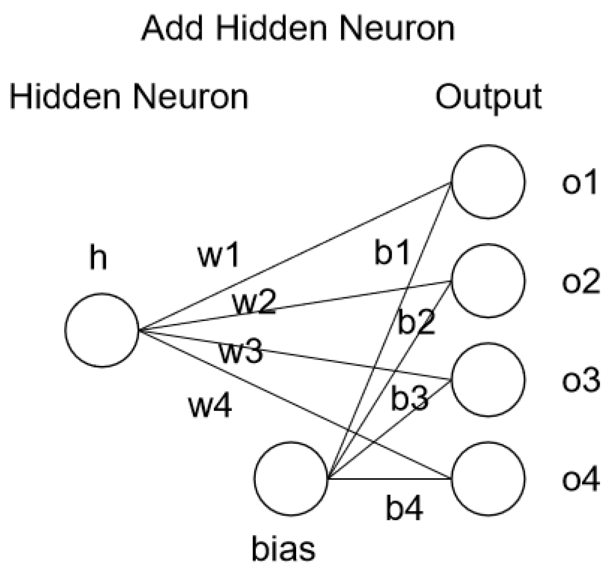
As shown in Figure 3, set n as the total number of training samples, h p as the output value of the hidden unit for the p-th training sample, o i , p as the output value of the i-th output unit for the p-th training sample, E p , o i as the error value between the true value of the p-th sample and the output of the i-th output unit, H = { h 1 , h 2 , , h n } as the set of hidden unit’s output value for all samples, E S oi = { E 1 , o i , E 2 , o i , , E n , o i } as the set of the i-th output unit’s error value for all samples.
In the traditional Cascade Correlation learning algorithm, the optimization goal of the hidden unit is S (Equation (6)). The value of S is maximized when the output fluctuations of the hidden unit coincide with the error fluctuations of the output unit.
The weight w acts to zoom in or out h p . If w is negative, h p can be reversed to change from negative to positive correlation. The bias b acts as floating the mean, ultimately maximizing the sum of absolute correlations between H and all E S o i , providing appropriate eigenvalues for the training of the following network. Howerver, the volatility of H may not necessarily be close to all E S o i at the same time.
Assuming that the output fluctuations of the newly added hidden unit h are consistent with the output unit o1, in other words, the output value of each sample can be converted:
w 1 * h p + b 1 = E p , o 1
Only if the remaining E S o i is in a proportion to E S o i ( E p , o 1 = E p , o i * k i + v i ), the newly added hidden unit may provide fully appropriate feature values for the remaining output units:
w 1 * h p + b 1 = E p , o i * k i + v i
Both sides except k:
w 1 k i * h p + b 1 v i k i = E p , o i
Appropriate values for and are as follows:
w i = w 1 k i , b i = b 1 v i k i
Obviously, this condition is not easy to achieve, and it is obvious that a hidden unit as a separate hidden layer to the network is limited. Therefore, the optimization targets of the hidden unit may be in conflict. Therefore, we present the improved Cascade Correlation neural network model based on a multi-objective group intelligent optimization algorithm. Each layer of the network consists of multiple hidden units, which improves the fitting ability of the problem for each layer. The multi-objective optimization method also alleviates the conflict among the hidden units.

4.2. MOEA-T Algorithm

We develop a modified multi-objective optimization algorithm named MOEA-T based on the idea of a cooperative multi-objective evolutionary algorithm with a propulsive population [39]. Because the general multi-objective optimization algorithm does not perform well in the improved Cascade Correlation neural network model, the final exploration depth is not enough. Therefore, MOEA-T first decomposes the multi-objective optimization problem into several single-object optimization problems based on several edge weights and optimizes them by using the jDE-B algorithm. After optimization, the optimal individuals will cover the individuals corresponding to the edge weights in the multi-objective optimization problem population. Then we implement a multi-objective optimization strategy for this population to evolve. Since the final required solution is mainly near the edge, and considering the time complexity problem, the EP archiving mechanism of MOEA/D was removed. The MOEA-T algorithm can explore sufficient depth in a short time, but with insufficient uniformity performance.
According to the Algorithm 2 idea, the specific steps of MOEA-T are as follows:
Algorithm 2. the specific steps of MOEA-T.
Require: Based on the number of optimized targets m, dividing the segmentation number H of per dimension, generate the uniformly distributed weight vector w, and the neighbor set Bi for each weight vector
Require: Generate m populations for edge search based on the edge weight vector, Pt = { P 1 , P 2 , , P m }
Require: Generate population Pm for multi-objective optimization, Pm = { x 1 , x 2 , , x N P } , each individual corresponds to a weight vector. The ideal point Z is determined from the optimal value under the different targets of the population.
1: for each P ∈ Pt do
2:     Population P was optimized with the jDE-B algorithm
3:     The best individual in P cover the corresponding individual in Pm
4: end for
5: while stopping criteria 2 is not met do
6:     for each i ∈ 1, 2, …, NP do
7:             Neighbor were selected for evolution operations
8:             Update ideal point Z
9:             Update the neighbor
10:  end for
11: end while
(1)
stopping criteria 2: Current iterations exceed the maximum specified value
(2)
Neighbors were selected for evolution operations: Two neighbors were randomly selected from the neighbor set Bi of the i-th individual to perform genetic manipulation with neighbors, yielding new trial individuals y1, y2, y3. The aggregation value (Equation (6)) is calculated according to the weight vector corresponding to the i-th individual, and the best aggregation value in the attempted individual is selected and compared with the original individual, and replaced if better.
g te ( x | λ i , z * ) = max 1 k m { λ k i | f k ( x ) z k * | }
(3)
Update ideal point Z: The evolved new individuals are compared with the ideal point Z under different optimization targets, and the ideal point Z is updated if there are better target values.
(4)
Update the neighbor: Traverse the neighbor set Bi and calculate the aggregate value of the i-th individual as well as the aggregate value of the neighbors based on the corresponding weight vector of each neighbor. If the aggregation value of the i-th individual is better, the neighbors are replaced and updated.
During the MOEA-T algorithm, the optimization objective of each propulsive population is a sub-objective of the multi-objective optimization problem. The optimization result is mainly affected by the corresponding weight vector. The multi-objective optimization population starts to initialize after the evolution of the propulsive population, and the optimal individuals in the propulsive populations are retained. Most of the optimal individuals in the population are the marginal solutions, which will affect the optimization direction and convergence speed of the remaining individuals. The final evolution results of the population in the MOEA-T algorithm may not be as uniformly distributed as in the MOEA/D algorithm. However, the MOEA-T algorithm can provide high-quality edge solutions in a relatively short time.

4.3. Improved Cascade Correlation Learning Algorithm Based on the MOEA-T Algorithm

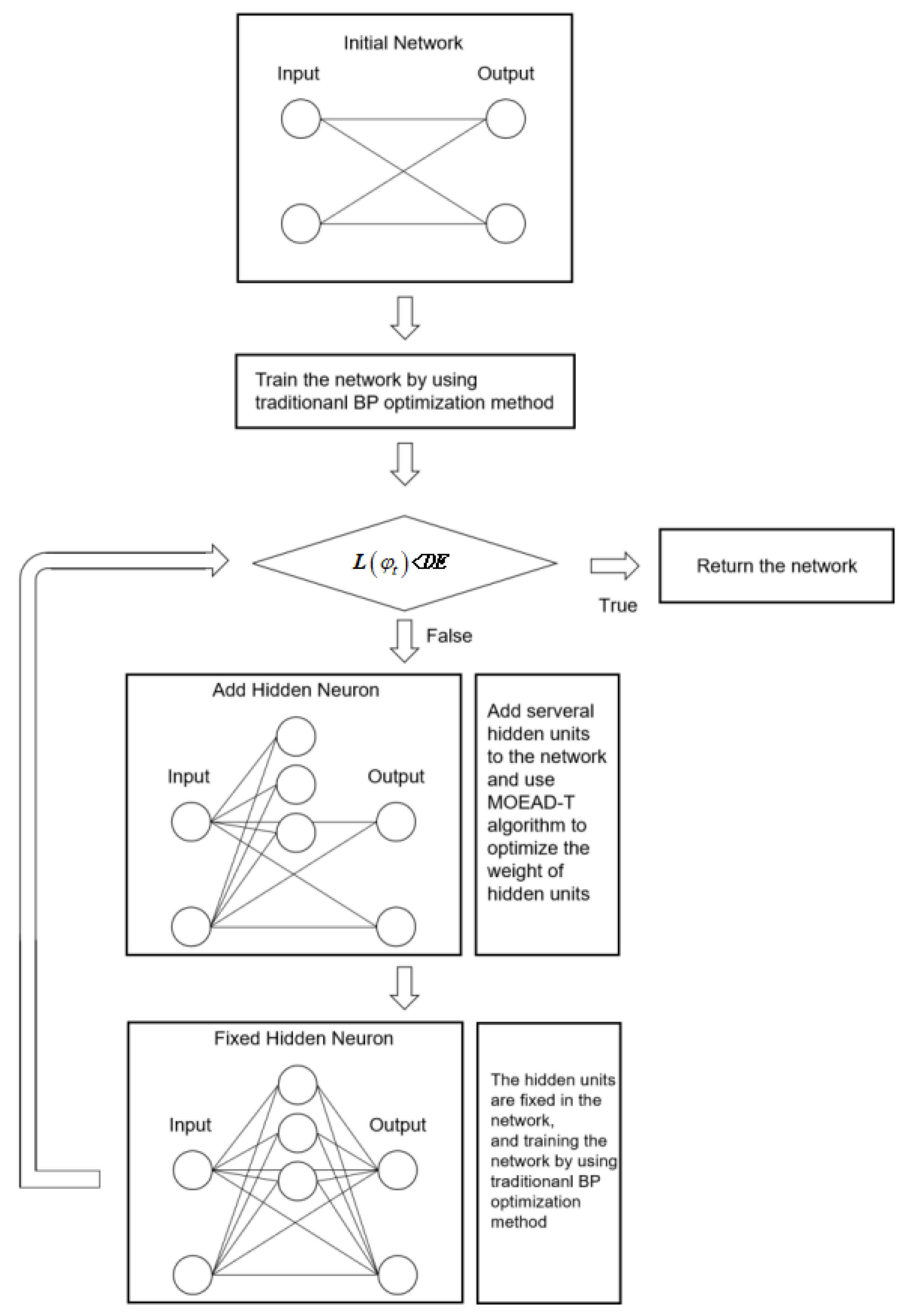
Since a hidden unit has a limited ability to fit output unit error correlation fluctuations, its optimization objective may conflict after being decomposed, this algorithm attempts to fit the error fluctuations required by the output unit in the training process with multiple hidden units. The network is no longer a hidden layer with only one hidden unit each time, but a hidden layer composed of multiple hidden units.
This algorithm adopts the MOEA-T multi-objective optimization algorithm in the stage of network training of hidden units. The number of optimization targets is generally determined by the number of output units, and several output units can also be artificially divided as one target. The optimization objective is to maximize S i , and thus to adjust the weight of the hidden units.
S o i = | p ( V p V ¯ ) ( E p , o i E ¯ o i ) |
S i = j S o j
V p is the output of the p-th sample in the hidden unit, V ¯ is the output average of all samples in the hidden unit, E p , o i is the error value between the true value of the p-th sample and the output of the i-th output unit, E ¯ o i is the error mean of the true values of all samples against the output of the i-th output unit, S o i is the absolute value of the correlation between the output of the hidden unit and the residual signal of the i-th output unit. S i is the optimization target. When an output unit acts as an optimization target, the optimization target is the absolute value of the correlation between the output of the hidden unit and the residual signal of the single output unit. When multiple output units are divided into one optimization target, the optimization target is the sum of the absolute values of the correlation between the output of the hidden unit and the divided output unit residual signal.
After the training of the MOEA-T algorithm, we select several solutions from the population as new hidden units to build them into new hidden layers. Specifically, the individuals corresponding to the edge weight were preferentially selected as the new hidden unit. Add a new hidden layer to the network, fix its input weight, and then connect to the output unit. Then we adjust the trainable weight with the traditional neural network training method to reduce the loss value. The termination condition of the CCNN-MOEA-T algorithm is that the current iterations are over the maximum iterations or the network loss value is less than the default error.
The specific algorithm process is shown in Figure 4.

5. Experimental Selection

The experiment was divided mainly into four parts. The first part verifies the effectiveness of the optimization algorithm strategy on the structure optimization of the Cascade Correlation neural network model. The second part verifies the effect of the multi-objective strategy on the deep optimization of the Cascaded Correlation neural network. The third part verifies the generality of the improved cascade correlation neural network algorithm proposed in this paper. The fourth part will try to reconstruct and optimize the fully connected layer of the classical image classification neural network model by using the improved Cascade Correlation learning algorithm.

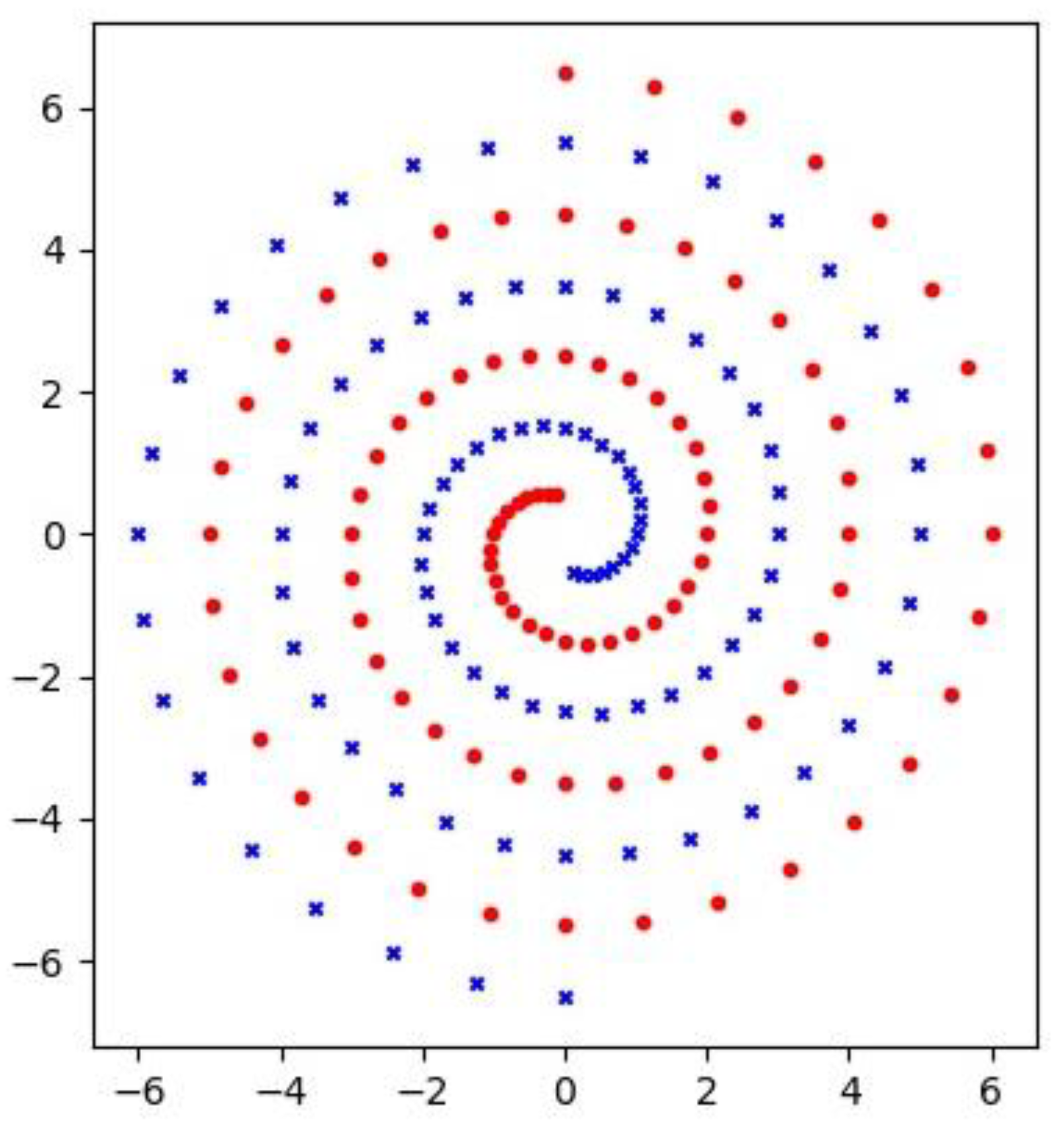
5.1. Two Spirals Classification Problem

The two spirals classification problem is a common benchmark in the data classification problem. As shown in Figure 5, there are two concentric spirals. The network should judge which spiral a given point belongs to. Traditional Cascade Correlation neural network models perform better than other general neural network models on this problem. This experiment will compare the CCNN-jDE-B algorithm with the standard Cascade Correlation learning algorithm and the CCNN-CSA-DE algorithm [16], which also adopts the population intelligence optimization strategy. Each algorithm will run 100 times on this problem, with the stop condition to correctly classify all samples of the problem. The average results of each algorithm on the problem are eventually shown.In addition to the above algorithms, the CCG-DLNN algorithm [2], the Sibling/Descendant CCNN algorithm, which adopts the cascade of correlated neural network learning strategy, and the GP-DLNN algorithm [1] is also selected.
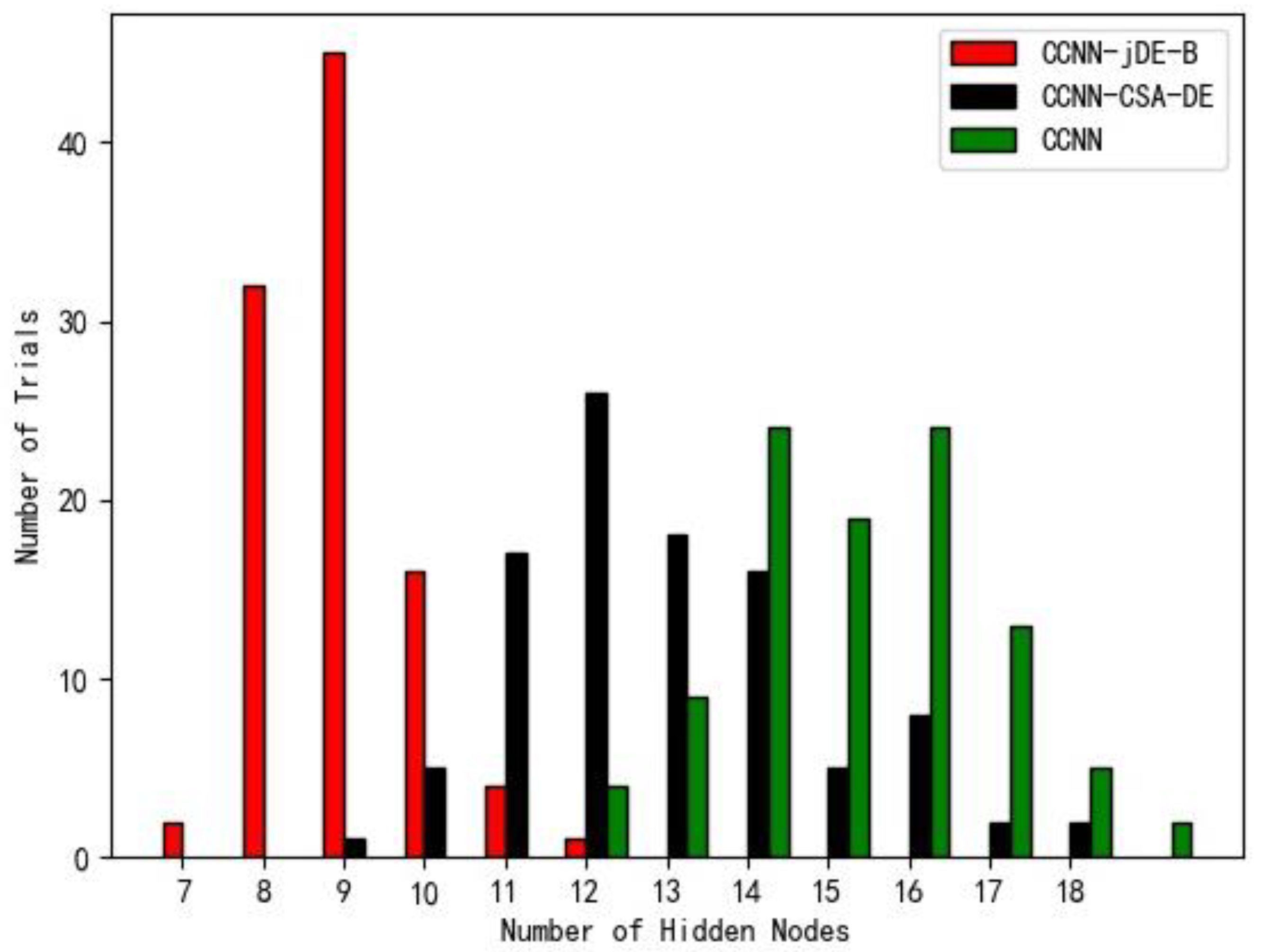
The experimental results in Table 1 show that the CCNN-jDE-B algorithm has faster convergence compared with other algorithms, and the final network structure is better. The CCNN-jDE-B algorithm is compared with traditional correlated neural network models, which proves that population intelligence optimization algorithms have significant results for training hidden units in Cascade Correlation neural network models, at the cost of possibly increased training time. The comparison of the CCNN-jDE-B algorithm and the CCNN-CSADE algorithm demonstrates the superiority of the jDE-B algorithm search strategy. As can be seen from Figure 6, the CCNN-jDE-B algorithm performs best depending on whether the jDE-B algorithm can better generate hidden units. The jDE-B algorithm has stronger global search ability and stability.

5.2. Four Spirals Classification Problem

5.2.1. Experimental Content

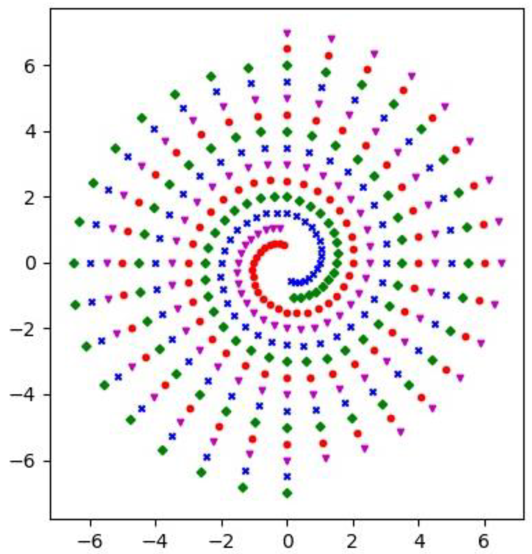
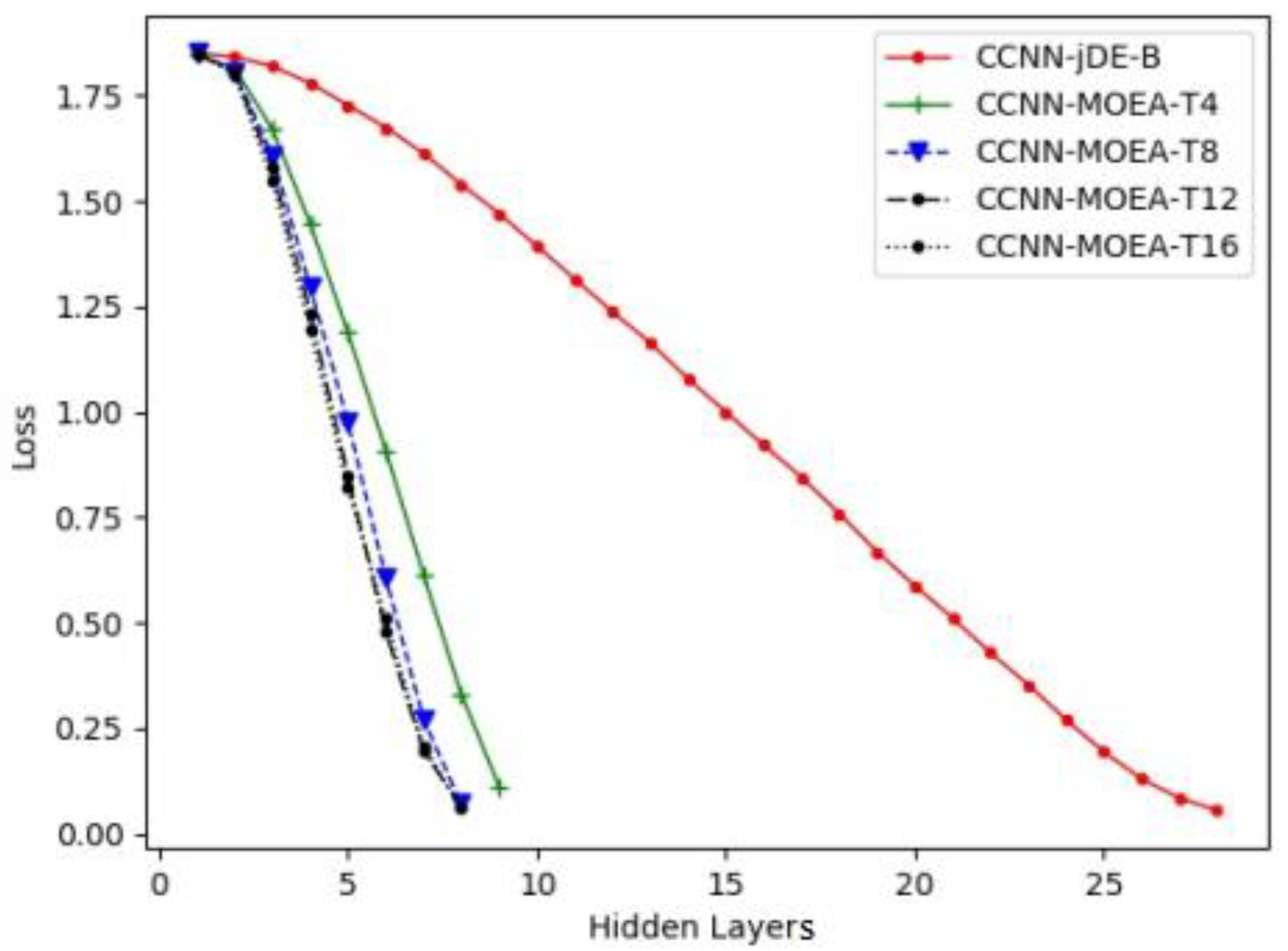
The four spirals classification problem is an upgraded version of the two spirals classification problem. As shown in Figure 7, there are four concentric spirals. The network should judge which spiral a given point belongs to. This problem tests the superiority of the multi-objective strategy and the optimization of the neural network model layer of the Cascade Correlation neural network. This experiment will run the standard Cascade Correlation learning algorithm, the CCNN-jDE-B algorithm and the CCNN-MOEA-T algorithm with different parameters. Each algorithm will run 25 times on this problem, each run with a stop condition for correctly classifying all samples of the problem. The final display is the average result of each algorithm on the problem and the loss value decrease diagram after the number of network layers increases.
As can be seen from Table 2, the final number of layers required for the improved multi-objective strategy is much lower on the four spirals problem than that based on the single-objective strategy. This shows that the correlation fluctuations fitted by the multi-objective strategy in each layer are better than those trained by a single hidden unit, but at the cost of generally a greater number of hidden units than a single target.
As can be seen from Figure 8, when comparing the multi-objective strategy, the more the number of hidden units is added in each layer, the faster the loss value of each layer of the network decreases. However, as the number of hidden units increases each time, this speed reaches an upper limit. That is to say, there is an upper limit on the correlation fluctuations simulated by each layer of the strategy, which cannot be fully fitted within one layer.

5.2.2. Comparison of Single-Object Optimization and Multi-Objective Optimization of Hidden Unit in Cascaded Correlation Neural Networks

When the network is in a certain training state, the errors required for different output units are different or even opposite. It is clearly insufficient to fit multiple output unit error fluctuations by only one hidden unit. The multiple hidden units trained based on the MOEAD-T algorithm have different weights than the output units. The ability of these hidden units to combine into a hidden layer will be better than a hidden layer composed of only one hidden unit.
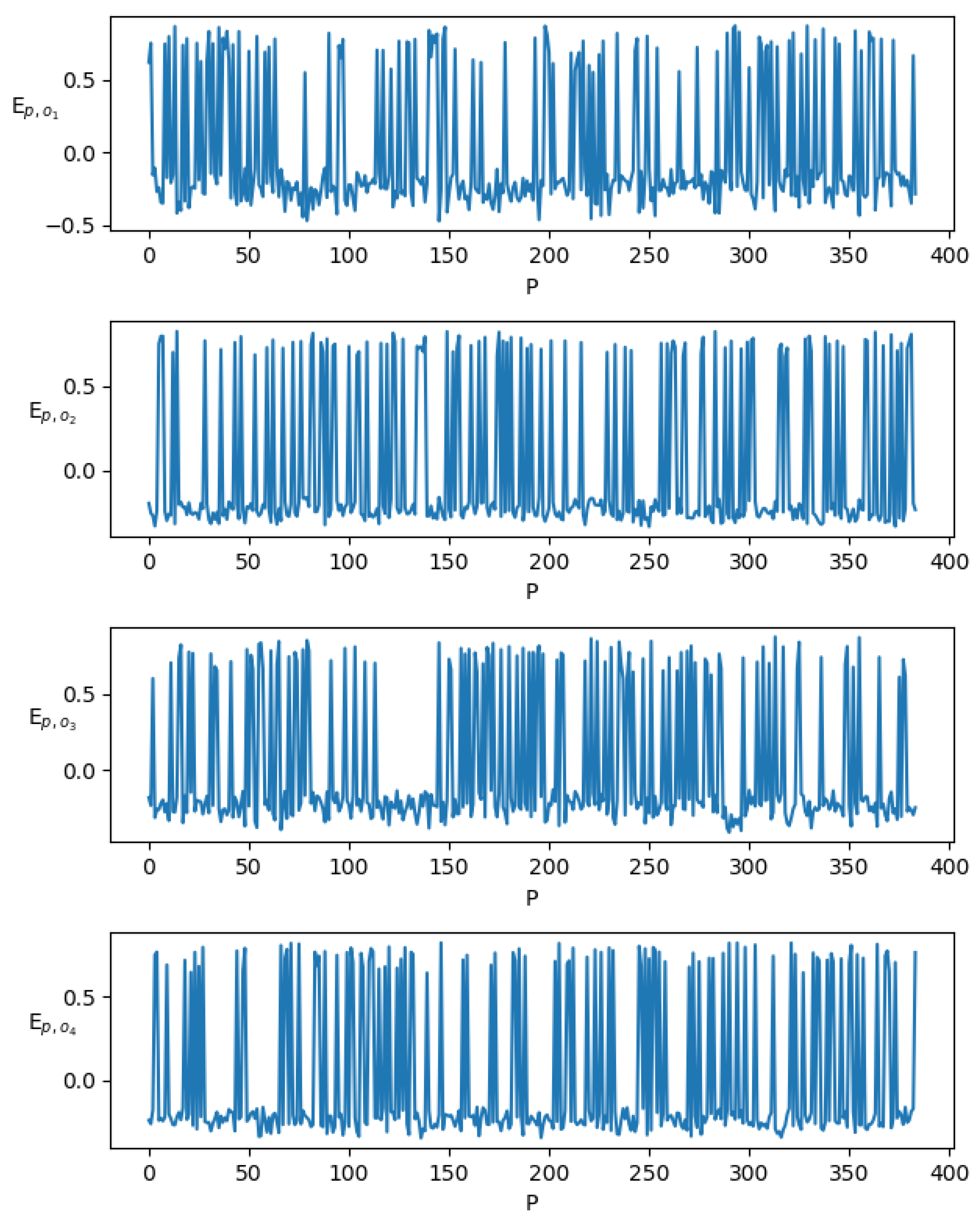
The training process of the cascading correlated neural network in solving the four-spiral classification problem is taken as an example. As shown in Figure 9, this is the error fluctuation of the four output units when the Cascade Correlation neural network tries to add the first hidden layer. P is the p-th sample, E p , o 1 is the error value of the p-th sample in the first output unit, E p , o 2 is the error value of the p-th sample in the second output unit, E p , o 3 is the error value of the p-th sample in the third output unit, E p , o 4 is the error value of the p-th sample in the fourth output unit.
When the jDE-B algorithm is adopted as the single-objective optimization method to fit the error fluctuations required for the above output units, the results are shown in Figure 10. P is the p-th sample, and S is the output value of the p-th sample in the hidden unit. The sum of the absolute values of the correlation between the output of the hidden unit and the residual signals of all the output units is S 65.72 , and others S o 1 30.92 , S o 2 10.03 , S o 3 22.83 , S o 4 1.94 .
When the MOEA-T algorithm is adopted as a multi-objective optimization method to fit the error fluctuations required by the above output units, the optimization target number is four, each output unit is divided into an independent optimization target, and finally four hidden units are added to a hidden layer. The results are shown in Figure 11, h 1 , p is the p-th sample, P is the output value of the p-th sample in the first hidden unit, h 2 , p is the output value of the p-th sample in the second hidden unit, h 3 , p is the output value of the p-th sample in the third hidden unit, h 4 , p is the output value of the p-th sample in the fourth hidden unit. During the first hidden unit, S 47.70 , S o 1 3.51 , S o 2 13.90 , S o 3 9.95 , S o 4 20.34 . During the second hidden unit, S 61.06 , S o 1 25.06 , S o 2 5.11 , S o 4 2.37 , S o 4 5.46 . During the third hidden unit, S 59.42 , S o 1 25.67 , S o 2 18.01 , S o 3 11.70 , S o 4 4.04 . During the fourth hidden unit, S 64.67 , S o 1 32.33 , S o 2 12.25 , S o 3 17.72 , S o 4 2.37 .
The best value for the four optimization targets in all hidden units is S o 1 32.33 , S o 2 18.01 , S o 3 25.42 , S o 4 20.34 . Simply connecting the hidden unit that contributes the most to the output unit to the output unit is also far more than a single target, S = S o 1 + S o 2 + S o 3 + S o 4 = 96.1 > 65.72 .
Moreover, the hidden unit will adjust the weight according to the traditional neural network optimization method, and make an appropriate contribution to the error reduction of other output units. It can be seen that the hidden layer added by the multi-objective optimization scheme can better fit the error fluctuation of the output unit and it can effectively reduce the loss value of the network.

5.3. The UCI Database Experiments

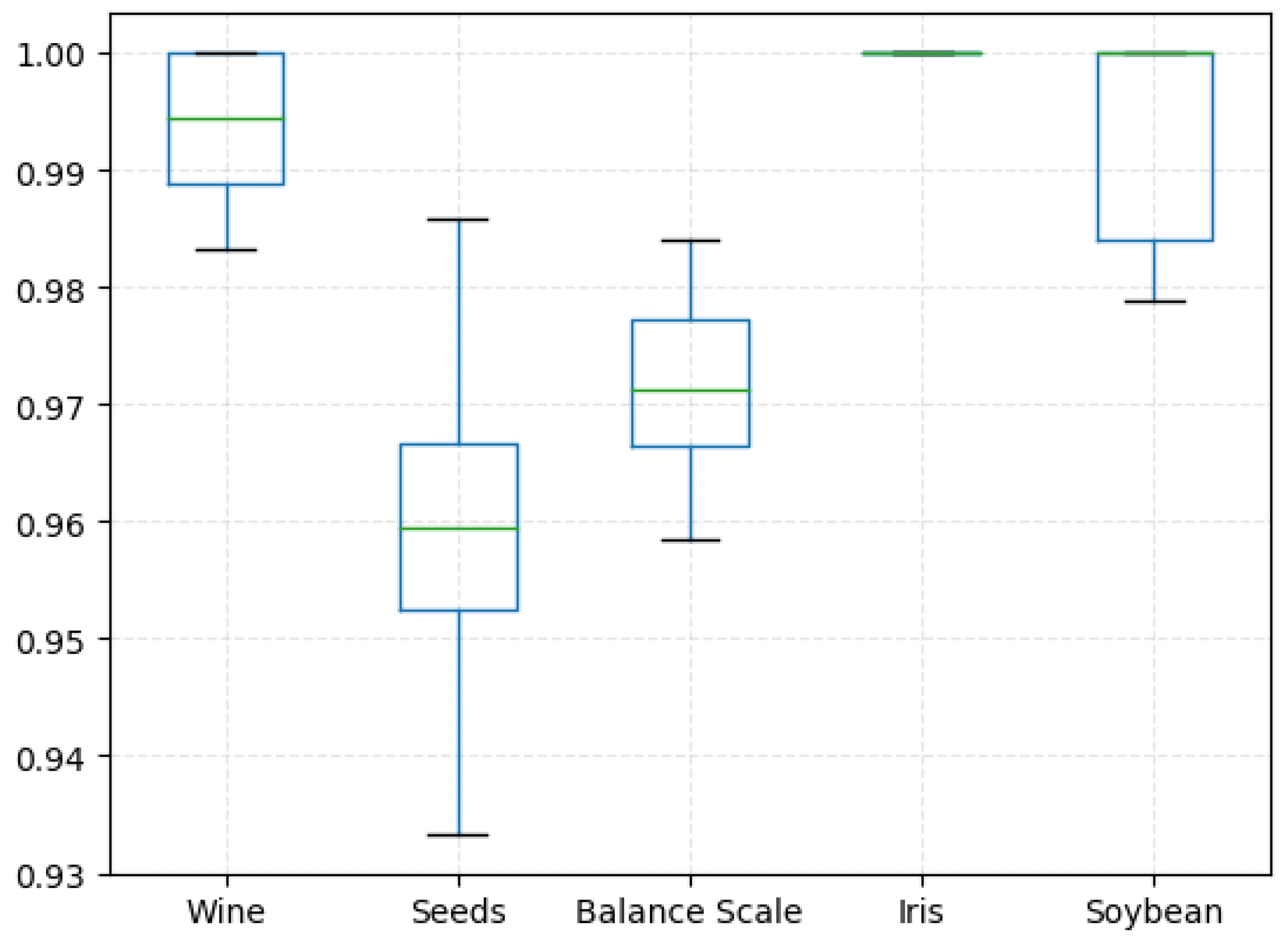
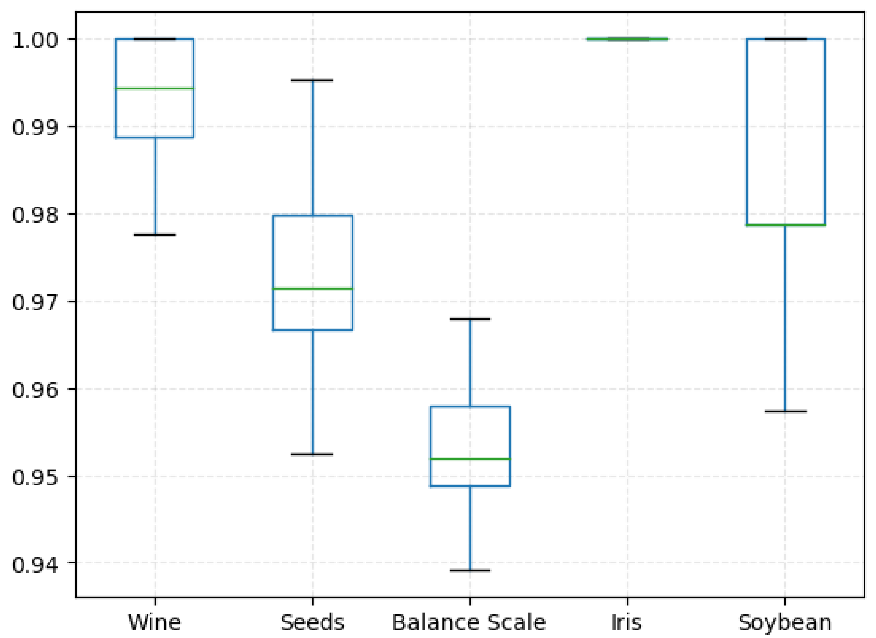
Experiments in this section will verify the generality of the CCNN-jDE-B algorithm and the CCNN-MOEA-T algorithm. The datasets used in the experiment are obtained from the UCI database. Five classical datasets were selected in this experiment, namely, Wine, Seeds, Balance Scale, Iris and Soybean. The datasets of Wine, record the chemical composition analysis of some wines in the same region of Italy. The analysis of each bottle shows they contain 13 ingredients, and these data can be divided into three wines. The datasets of Seeds, with the information characteristics of seven wheat seeds, can be classified into three wheat seeds. The datasets of the Balance Scale, with four kinds of Libra placement information, respectively, the distance and weight of the left and right end, can be divided into three kinds of placement results. The datasets of Iris, with the informative characteristics of four iris species, can be divided into three species of iris. The datasets of Soybean, with 35 kinds of soybean growth information characteristics, can be classified into four kinds of diseased soybeans. Relevant information for each dataset is shown in the Table 3. The experiment will perform ten cross-validations of each dataset using the CCNN-jDE-B algorithm. The classification accuracy was used as the main evaluation index.
The results of each algorithm in this experiment are shown in the Table 4 and Table 5.
It can be seen from the experimental results in Figure 12 and Figure 13. The CCNN-jDE-B algorithm performs well on each datasets, and can build a better network m`odel with high accuracy. The CCNN-MOEA-T algorithm also performs well on each datasets, and can build a shallow network model with high accuracy. However, when the number of training samples is insufficient, the training of the network tends to cause overfitting. It performs very well on the training set and performs relatively poorly on the test set. This is also the reason why the CCNN-jDE-B algorithm and the CCNN-MOEA-T algorithm performs differently on some datasets.

5.4. The CIFAR-10 Classification Problem

The CIFAR-10 dataset is divided into 10 species, each with 6000 images, and includes a total of 60,000 32 × 32 color images. Among them, the datasets were divided into 50,000 training images and 10,000 test images. In this experiment, the LeNet-5 [40] network and the AlexNet [41] network are pretrained. Then the connection layer is removed and the convolutional layer is extracted as the input unit of the Cascade Correlation neural network. Finally, the Cascade Correlation learning algorithm is used to construct a new connection layer. The experiment will compare the results of the fully connected layer by using different Cascade Correlation learning algorithms.
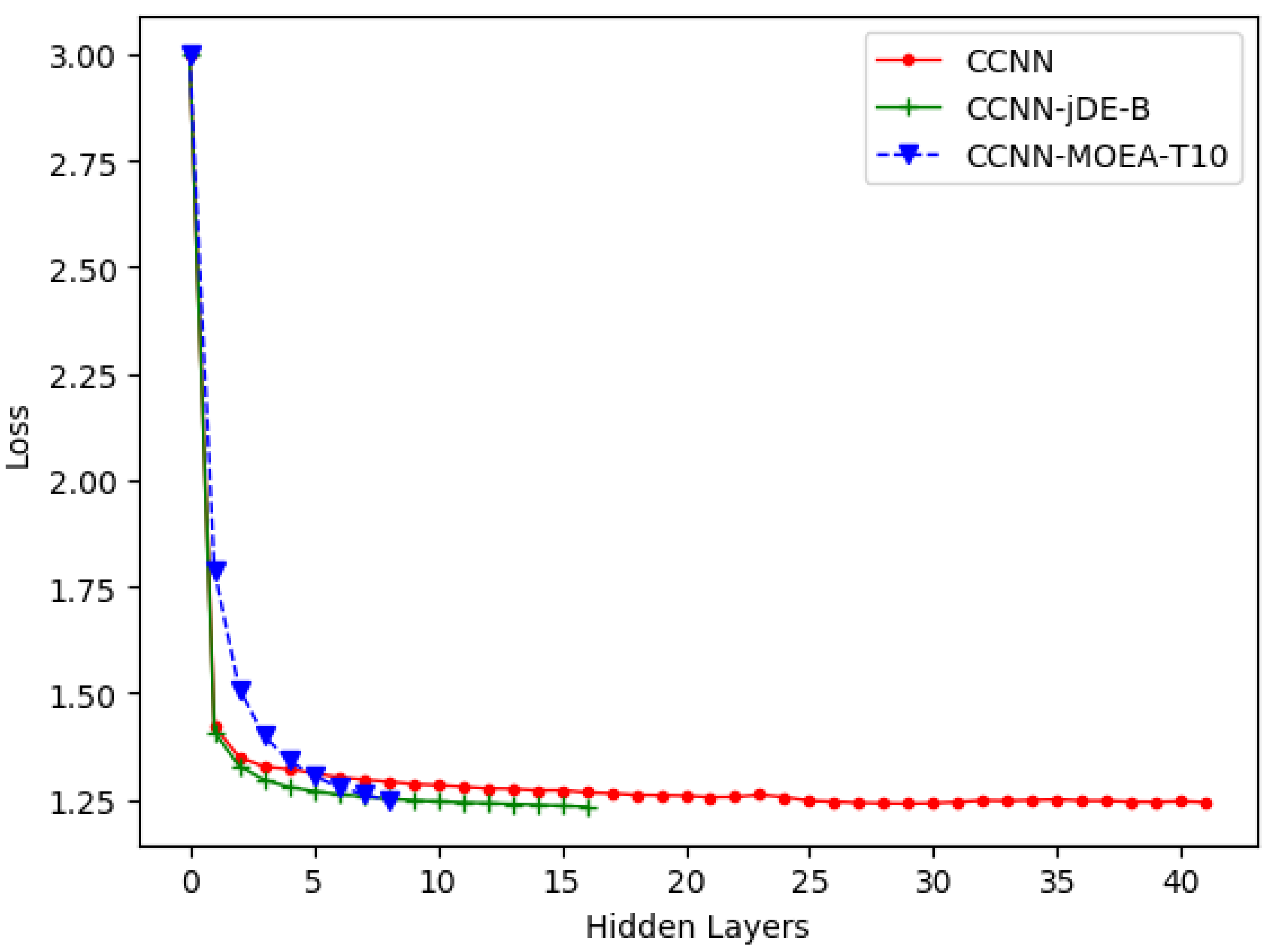
From the experimental results of the LeNet-5 network pretraining and reconstruction in Table 6, we show that the LeNet-5 network model is limited by the network size and has only achieved about 60% accuracy on the CIFAR-10 datasets. Image features of the CIFAR-10 datasets are relatively complex. The training data are relatively insufficient. The convolutional layer of the LeNet-5 network has a limited ability to extract picture features. The convolutional layer is used to extract the picture features, and then the Cascade Correlation learning algorithm is used to construct the connection layer. As can be seen from Table 6, the constructed network structure is smaller than the original network structure, but the accuracy is difficult to improve. As can be seen from Figure 14, the loss value of each algorithm decreases at a different speed when the extracted features are limited.
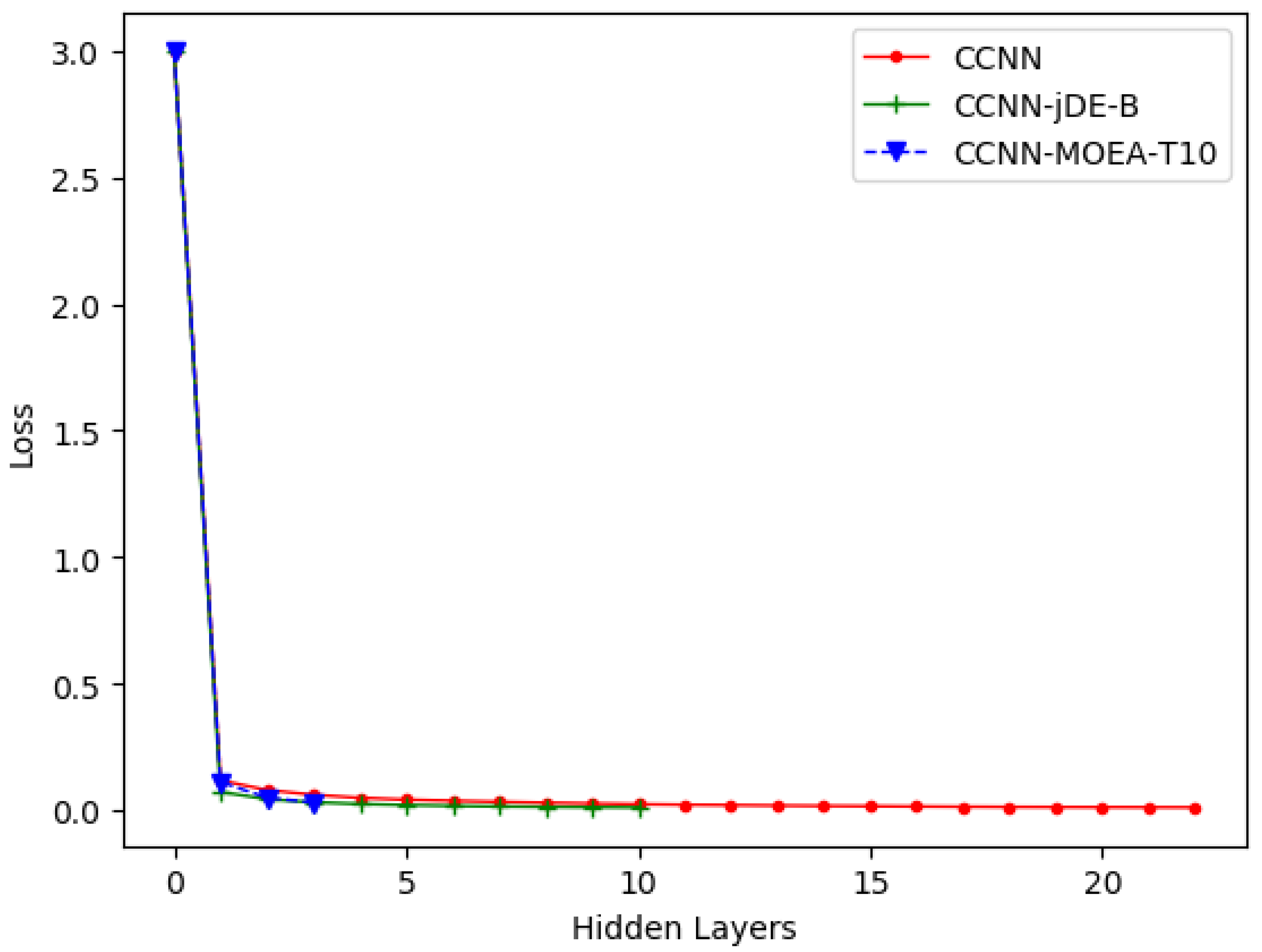
The experimental results of the AlexNet network pre-training and reconstruction in Table 7 show that the network model is too large and overfitted on the training set of the CIFAR-10 datasets. The image features of the CIFAR-10 datasets are more complex, while the training data is relatively insufficient. Although the accuracy of the training set can continue to improve with continued training, the accuracy of the test set will not. Therefore, this experiment adopts the network model that achieves the highest accuracy in the test set in the training process. The convolutional layer is used to extract the picture features, and then the Cascade Correlation learning algorithm is used to construct the connection layer. Finally, the constructed network structure is smaller than the original network structure, but the accuracy is difficult to improve. As can be seen from Figure 15, the loss value of each algorithm decreases at the same speed when the extracted features are sufficient.
Since the AlexNet network is prone to overfitting on the CIFAR-10 dataset, the following experiments adopt data augmentation methods. The training set pictures will be randomly changed to enhance the image features. According to the training results, although the overfitting phenomenon still appeared, the test set accuracy improved. This experiment adopts the model that achieves the highest accuracy in the training set. The convolutional layer is used to extract the picture features, and then the Cascade Correlation learning algorithm is used to construct the connection layer. As can be seen from Table 8, the number of hidden units constructed in the current experiment is greatly reduced compared with the previous experimental model.

6. Conclusions

In this paper, we propose the single-objective optimization algorithm jDE-B and the multi-objective optimization algorithm MOEA-T, and improve the network expansion mode in the learning process of the Cascade Correlation neural network. The improved Cascade Correlation learning algorithm based on the jDE-B algorithm finds the global optimal solution with greater probability in the hidden unit training stage. Since the Cascade Correlation neural networks will fix their input weights after adding hidden units, good global solutions reduce the number of hidden units, reducing the final network size. The modified Cascade Correlation learning algorithm based on the MOEA-T algorithm uses multiple hidden units to fit the error fluctuations required for the output units during training. The network is no longer a hidden layer with only one hidden unit each time, but a hidden layer composed of multiple hidden units. Compared with the single-objective optimization scheme, it can better fit the error fluctuations of the output units, effectively reduce the loss value of the network, and reduce the final network depth. Furthermore, the shortcomings of single-objective schemes are analyzed through comparison with multi-objective schemes and validated by experiments. Finally, our future research may be to refer to other effective strategies to improve the Cascade Correlation neural network for solving decision-making problems.

Author Contributions

Methodology, W.W.; Software, J.D.; Formal analysis, Q.L.; Data curation, J.D.; Writing—original draft, J.D.; Writing—review & editing, Q.L. and W.W.; Supervision, W.W. All authors have read and agreed to the published version of the manuscript.

Funding

The Key Project of Science and Technology Innovation 2030 supported by the Ministry of Science and Technology of China (No. 2018AAA0101301), the Key Projects of Artificial Intelligence of High School in Guangdong Province (No. 2019KZDZX1011) and The High School innovation Project (No. 2018KTSCX222).

Institutional Review Board Statement

Not applicable.

Informed Consent Statement

Not applicable.

Data Availability Statement

The all data presented in the article does not require copyright. They are freely available from the authors.

Acknowledgments

The author appreciated very much attention and support of my submission by anonymous editor as well as concrete and profound comments of the reviewers.

Conflicts of Interest

The authors declare no conflict of interest.

References

  1. Zemouri, R.; Omri, N.; Fnaiech, F.; Zerhouni, N.; Fnaiech, N. A new growing pruning deep learning neural network algorithm (GP-DLNN). Neural Comput. Appl. 2019, 32, 18143–18159. [Google Scholar] [CrossRef]
  2. Mohamed, E.M.; Mohamed, M.H.; Farghally, M.F. A New Cascade-Correlation Growing Deep Learning Neural Network Algorithm. Algorithms 2021, 14, 158. [Google Scholar] [CrossRef]
  3. Qiao, J.; Li, F.; Han, H.; Li, W. Constructive algorithm for fully connected cascade feedforward neural networks. Neurocomputing 2015, 182, 154–164. [Google Scholar] [CrossRef]
  4. Zhang, R.; Lan, Y.; Huang, G.B.; Xu, Z.B. Universal Approximation of Extreme Learning Machine with Adaptive Growth of Hidden Nodes. IEEE Trans. Neural Netw. Learn. Syst. 2012, 23, 365–371. [Google Scholar] [CrossRef]
  5. Shahjahan, M.; Murase, K. A constructive algorithm for training cooperative neural network ensembles. IEEE Trans. Neural Netw. 2003, 14, 820–834. [Google Scholar]
  6. Augasta, M.G.; Kathirvalavakumar, T. A Novel Pruning Algorithm for Optimizing Feedforward Neural Network of Classification Problems. Neural Process. Lett. 2011, 34, 241. [Google Scholar] [CrossRef]
  7. Qiao, J.F.; Zhang, Y.; Han, H.G. Fast unit pruning algorithm for feedforward neural network design. Appl. Math. Comput. 2008, 205, 622–627. [Google Scholar] [CrossRef]
  8. Han, H.G.; Qiao, J.F. A structure optimisation algorithm for feedforward neural network construction. Neurocomputing 2013, 99, 347–357. [Google Scholar] [CrossRef]
  9. Wan, W.; Mabu, S.; Shimada, K.; Hirasawa, K.; Hu, J. Enhancing the generalization ability of neural networks through controlling the hidden layers. Appl. Soft Comput. 2009, 9, 404–414. [Google Scholar] [CrossRef]
  10. Han, H.G.; Zhang, S.; Qiao, J.F. An Adaptive Growing and Pruning Algorithm for Designing Recurrent Neural Network. Neurocomputing 2017, 242, 51–62. [Google Scholar] [CrossRef]
  11. Narasimha, P.L.; Delashmit, W.H.; Manry, M.T.; Li, J.; Maldonado, F. An integrated growing-pruning method for feedforward network training. Neurocomputing 2008, 71, 2831–2847. [Google Scholar] [CrossRef]
  12. Fahlman, S.E.; Lebiere, C. The Cascade-Correlation Learning Architecture. In Advances in Neural Information Processing Systems; Morgan Kaufmann Pub.: San Francisco, CA, USA, 1990. [Google Scholar]
  13. Guo, Y.; Liang, B.; Lao, S.; Wu, S.; Lew, M.S. A Comparison between Artificial Neural Network and Cascade-Correlation Neural Network in Concept Classification; Springer International Publishing: Berlin, Germany, 2014. [Google Scholar]
  14. Huang, G.; Song, S.; Wu, C. Orthogonal Least Squares Algorithm for Training Cascade Neural Networks. IEEE Trans. Circuits Syst. I Regul. Pap. 2012, 59, 2629–2637. [Google Scholar] [CrossRef]
  15. Marquez, E.S.; Hare, J.S.; Niranjan, M. Deep Cascade Learning. IEEE Trans. Neural Netw. Learn. Syst. 2018, 29, 5475–5485. [Google Scholar] [CrossRef] [PubMed]
  16. Gao, X.Z.; Wang, X.; Ovaska, S.J. Fusion of clonal selection algorithm and differential evolution method in training cascade–correlation neural network. Neurocomputing 2009, 72, 2483–2490. [Google Scholar] [CrossRef]
  17. Li, H.; Hu, C.X.; Li, Y. The BP neural network model and application based on genetic algorithm. In Proceedings of the 2011 International Conference on Electric Information and Control Engineering, Wuhan, China, 15–17 April 2011; IEEE: Berkeley, CA, USA; pp. 795–798. [Google Scholar]
  18. Qi, C.; Bi, Y.; Yong, L. Improved BP neural network algorithm model based on chaos genetic algorithm. In Proceedings of the 2017 3rd IEEE International Conference on Control Science and Systems Engineering (ICCSSE), Beijing, China, 17–19 August 2017; IEEE: Berkeley, CA, USA; pp. 679–682. [Google Scholar]
  19. Storn, R.; Price, K. Differential Evolution—A Simple and Efficient Heuristic for global Optimization over Continuous Spaces. J. Glob. Optim. 1997, 11, 341–359. [Google Scholar] [CrossRef]
  20. Brest, J.; Greiner, S.; Boskovic, B.; Mernik, M.; Zumer, V. Self-Adapting Control Parameters in Differential Evolution: A Comparative Study on Numerical Benchmark Problems. IEEE Trans. Evol. Comput. 2006, 10, 646–657. [Google Scholar] [CrossRef]
  21. Wang, B.C.; Li, H.X.; Zhang, Q.F.; Wang, Y. Decomposition-based multiobjective optimization for constrained evolutionary optimization. IEEE Trans. Syst. Man Cybern. Syst. 2021, 51, 574–587. [Google Scholar] [CrossRef]
  22. Trivedi, A.; Srinivasan, D.; Sanyal, K.; Ghosh, A. A Survey of Multiobjective Evolutionary Algorithms Based on Decomposition. IEEE Trans. Evol. Comput. 2017, 21, 440–462. [Google Scholar] [CrossRef]
  23. Asafuddoula, M.; Ray, T.; Sarker, R. A Decomposition-Based Evolutionary Algorithm for Many Objective Optimization. IEEE Trans. Evol. Comput. 2015, 19, 445–460. [Google Scholar] [CrossRef]
  24. Xu, B.; Zhang, Y.; Gong, D.; Guo, Y.; Rong, M. Environment Sensitivity-Based Cooperative Co-Evolutionary Algorithms for Dynamic Multi-Objective Optimization. IEEE/ACM Trans. Comput. Biol. Bioinform. 2018, 15, 1877–1890. [Google Scholar] [CrossRef]
  25. Lee, S.-W. Optimisation of the cascade correlation algorithm to solve the two-spiral problem by using CosGauss and Sigmoid activation functions. Int. J. Intell. Inf. Database Syst. 2014, 8, 97–115. [Google Scholar] [CrossRef]
  26. Baluja, S.; Fahlman, S.E. Reducing Network Depth in the Cascade-Correlation Learning Architecture; Carnegie Mellon University: Pittsburgh, PA, USA, 1994. [Google Scholar]
  27. Wang, Z.; Khan, W.A.; Ma, H.L.; Wen, X. Cascade neural network algorithm with analytical connection weights determination for modelling operations and energy applications. Int. J. Prod. Res. 2020, 58, 7094–7111. [Google Scholar] [CrossRef]
  28. Ghorbani, M.A.; Deo, R.C.; Kim, S.; Kashani, M.H.; Karimi, V.; Izadkhah, M. Development and evaluation of the cascade correlation neural network and the random forest models for river stage and river flow prediction in Australia. Soft Comput. 2020, 24, 12079–12090. [Google Scholar] [CrossRef]
  29. Elbisy, M.S.; Ali, H.M.; Abd-Elall, M.A.; Alaboud, T.M. The use of feed-forward back propagation and cascade correlation for the neural network prediction of surface water quality parameters. Water Resour. 2014, 41, 709–718. [Google Scholar] [CrossRef]
  30. Velusamy, K.; Amalraj, R. Performance of the cascade correlation neural network for predicting the stock price. In Proceedings of the 2017 Second International Conference on Electrical, Computer and Communication Technologies (ICECCT), Coimbatore, India, 22–24 February 2017. [Google Scholar]
  31. Das, S.; Suganthan, P.N. Differential Evolution: A Survey of the State-of-the-Art. IEEE Trans. Evol. Comput. 2011, 15, 4–31. [Google Scholar] [CrossRef]
  32. Neri, F.; Tirronen, V. Recent advances in differential evolution: A survey and experimental analysis. Artif. Intell. Rev. 2010, 33, 61–106. [Google Scholar] [CrossRef]
  33. Das, S.; Mullick, S.S.; Suganthan, P.N. Recent advances in differential evolution—An updated survey. Swarm Evol. Comput. 2016, 27, 1–30. [Google Scholar] [CrossRef]
  34. Zhang, J.; Sanderson, A.C. JADE: Adaptive Differential Evolution with Optional External Archive. IEEE Trans. Evol. Comput. 2009, 13, 945–958. [Google Scholar] [CrossRef]
  35. Zhang, Q.; Hui, L. MOEA/D: A Multiobjective Evolutionary Algorithm Based on Decomposition. IEEE Trans. Evol. Comput. 2008, 11, 712–731. [Google Scholar] [CrossRef]
  36. Deb, K.; Pratap, A.; Agarwal, S.; Meyarivan, T. A fast and elitist multiobjective genetic algorithm: NSGA-II. IEEE Trans. Evol. Comput. 2002, 6, 182–197. [Google Scholar]
  37. Deb, K.; Jain, H. An Evolutionary Many-Objective Optimization Algorithm Using Reference-Point-Based Nondominated Sorting Approach, Part I: Solving Problems with Box Constraints. IEEE Trans. Evol. Comput. 2014, 18, 577–601. [Google Scholar] [CrossRef]
  38. Jain, H.; Deb, K. An Evolutionary Many-Objective Optimization Algorithm Using Reference-Point Based Nondominated Sorting Approach, Part II: Handling Constraints and Extending to an Adaptive Approach. IEEE Trans. Evol. Comput. 2014, 18, 602–622. [Google Scholar] [CrossRef]
  39. Wang, J.; Li, Y.; Zhang, Q.; Zhang, Z.; Gao, S. Cooperative Multiobjective Evolutionary Algorithm with Propulsive Population for Constrained Multiobjective Optimization. IEEE Trans. Syst. Man Cybern. Syst. 2021, 52, 3476–3491. [Google Scholar] [CrossRef]
  40. Lécun, Y.; Bottou, L.; Bengio, Y.; Haffner, P. Gradient-based learning applied to document recognition. Proc. IEEE 1998, 86, 2278–2324. [Google Scholar] [CrossRef]
  41. Krizhevsky, A.; Sutskever, I.; Hinton, G.E. Imagenet classification with deep convolutional neural networks. Commun. ACM 2017, 60, 84–90. [Google Scholar] [CrossRef] [Green Version]
Figure 1. Training process of the Cascade Correlation Neural network.
Axioms 12 00164 g001
Figure 2. Steps of CCNN-jDE-B algorithm.
Axioms 12 00164 g002
Figure 3. The hidden unit provides suitable features to the network.
Axioms 12 00164 g003
Figure 4. Steps of CCNN-MOEA-T algorithm.
Axioms 12 00164 g004
Figure 5. The two spirals classification problem.
Axioms 12 00164 g005
Figure 6. Distribution of the number of hidden units of each algorithm on the two spirals classification problem.
Axioms 12 00164 g006
Figure 7. Four spirals classification problem.
Axioms 12 00164 g007
Figure 8. Each algorithm drops the loss value on the four spirals classification problem.
Axioms 12 00164 g008
Figure 9. The error fluctuations of output units during training.
Axioms 12 00164 g009
Figure 10. The single objective method fits the output unit’s fluctuations during training.
Axioms 12 00164 g010
Figure 11. The multi-objective method fits the output unit’s fluctuations during training.
Axioms 12 00164 g011
Figure 12. The distribution of the accuracy rates of the CCNN-jDE-B algorithm tests in each dataset.
Axioms 12 00164 g012
Figure 13. The distribution of the accuracy rates of the CCNN-MOEA-T algorithm tests in each datasets.
Axioms 12 00164 g013
Figure 14. Loss value drop diagram.
Axioms 12 00164 g014
Figure 15. Loss value drop diagram.
Axioms 12 00164 g015
Table 1. The simulation results of each algorithm on the two spirals classification problem.
CCNN-
jDE-B
CCNNCCNN-
CSA-DE
CCG-
DLNN
GP-
DLNN
Sibling/Descendant CCNN
Hidden Units8.9215.212.9227014.6
Hidden Layers8.9215.212.9237.3
Accuracy100%100%100%99.5%92.23%100%
Table 2. The simulation results of each algorithm on the four spirals classification problem.
AlgorithmHidden UnitsHidden LayersAccuracy
CCNN39.539.5100%
CCNN-jDE-B27.5227.52100%
CCNN-MOEA-Tm = 436.89.2100%
m = 862.727.84100%
m = 1292.167.68100%
m = 16122.247.64100%
Sibling/Descendant CCNN λ = 1.039.228.2100%
λ = 0.9543.323.8100%
λ = 0.939.921.2100%
λ = 0.840.914.2100%
Table 3. Data and Characteristics.
DatasetSample SizeCharacteristics NumberClassification Number
Wine178133
Seeds21073
Balance Scale62543
Iris15043
Soybean47354
Table 4. The simulation results of the CCNN-jDE-B algorithm.
DatasetMaximum AccuracyMinimum AccuracyAverage AccuracyAverage Number of Hidden UnitsAverage Number of Hidden Layers
Wine100%98.31%99.37%11
Seeds98.57%93.33%95.90%4.94.9
Balance Scale98.40%95.84%97.12%8.088.08
Iris100%98.66%99.95%11
Soybean100%93.61%99.23%4.244.24
Table 5. The simulation results of the CCNN-MOEA-T algorithm.
DatasetMaximum AccuracyMinimum AccuracyAverage AccuracyAverage Number of Hidden UnitsAverage Number of Hidden Layers
Wine100%97.75%99.29%31
Seeds99.52%95.23%97.22%3.421.14
Balance Scale96.80%93.92%95.31%17.165.72
Iris100%98.00%99.74%3.421.14
Soybean100%93.61%98.12%10.962.74
Table 6. The simulation results of the LeNet-5 pre-training and reconstruction on the CIFAR-10 classification.
LeNet-5CCNNCCNN-jDE-BCCNN-MOEA-T
Number of hidden units in the connection layer204401570
Number of connected layers240157
Training set accuracy60.3%60.7%60.9%60.8%
Test set accuracy58.1%57.1%57.8%56.7%
Table 7. The simulation results of the AlexNet pre-training and reconstruction on the CIFAR-10 classification.
AlexNetCCNNCCNN-jDE-BCCNN-MOEA-T
Number of hidden units in the connection layer12,28821920
Number of connected layers32192
Training set accuracy93.2%99.9%99.9%99.7%
Test set accuracy78.8%77.4%77.9%76.7%
Table 8. The simulation results of the AlexNet pre-training and reconstruction on the CIFAR-10 classification under data augmentation.
AlexNetCCNNCCNN-jDE-BCCNN-MOEA-T10
Number of hidden units in the connection layer12,2885210
Number of connected layers3521
Training set accuracy100%100%100%100%
Test set accuracy85.6%82.6%83.1%81.2%
Disclaimer/Publisher’s Note: The statements, opinions and data contained in all publications are solely those of the individual author(s) and contributor(s) and not of MDPI and/or the editor(s). MDPI and/or the editor(s) disclaim responsibility for any injury to people or property resulting from any ideas, methods, instructions or products referred to in the content.