An Expectation-Maximization Algorithm for Combining a Sample of Partially Overlapping Covariance Matrices

Abstract

The generation of unprecedented amounts of data brings new challenges in data management, but also an opportunity to accelerate the identification of processes of multiple science disciplines. One of these challenges is the harmonization of high-dimensional unbalanced and heterogeneous data. In this manuscript, we propose a statistical approach to combine incomplete and partially-overlapping pieces of covariance matrices that come from independent experiments. We assume that the data are a random sample of partial covariance matrices sampled from Wishart distributions and we derive an expectation-maximization algorithm for parameter estimation. We demonstrate the properties of our method by (i) using simulation studies and (ii) using empirical datasets. In general, being able to make inferences about the covariance of variables not observed in the same experiment is a valuable tool for data analysis since covariance estimation is an important step in many statistical applications, such as multivariate analysis, principal component analysis, factor analysis, and structural equation modeling.

1. Introduction

High-throughput measurement technologies have revolutionized many scientific disciplines by decreasing the time and cost of analyzing multiple samples and generating huge amounts of data, which has created great opportunities single degreesbut also brought new challenges, especially in data cleaning, normalization, dimension reduction, data harmonization, and data storage. The challenge we want to address in this manuscript is the integration of data from different sources by making inferences about the covariance of variables not observed in the same experiment. Covariance estimation is an important step in many statistical applications, such as multivariate analysis, principal component analysis, factor analysis, structural equation modeling, and statistical genomics.

Harmonization of the increasing amounts of datasets that accumulate in databases has great potential to accelerate our understanding of scientific processes. One of the challenges that still needs to be addressed is the incompleteness inherent in scientific data, in other words, each dataset that is the result of an experimental or observational study can address a limited number of variables with a limited number of samples. The lack of a large sample size reduces the reproducibility of the study [1], and the lack of a large number of measured variables narrows the scope of the study. The integration of information from different datasets is required to accelerate the identification of significant scientific outcomes.

Modern data integration approaches include feature imputation, conventional meta-analysis [2,3,4,5] and many other new methods based on machine learning and statistical methods [6,7,8,9,10,11]. Detailed reviews and classifications of some promising statistical approaches for data integration can be found in [12,13,14]. The results in these studies demonstrate the advantage of integrating multiple diverse datasets.

This work describes a method for learning the covariances among a set of variables by combining multiple covariance matrices from independent experiments. Our method is closely related to meta-analytic structural equation modeling (MASEM). MASEM is a two-stage approach to estimating the parameters of a structural equation model (SEM) using covariance matrices from different studies [15,16]. The first stage of MASEM is to pool the covariance matrices from the different studies, and the second stage is to estimate the parameters of the SEM using the pooled covariance matrix. Our method can be used in the first stage of MASEM to pool the covariance matrices from the different studies.

The main advantage of our method over the existing techniques for pooling covariances is that we use the expectation-maximization algorithm to maximize the likelihood function, leading to an analytical solution for each iteration of the algorithm. This makes our algorithm computationally efficient and suitable for combining covariance matrices involving many variables. In contrast, the existing MASEM methods for pooling covariances are based on iterative algorithms, which directly maximize the likelihood function over the parameters of the covariance matrix. Since the number of parameters in the covariance matrix is quadratic in the number of variables, these methods become more computationally demanding for large numbers of variables. We compared the performance of our method to the performance of the first stage of two-stage MASEM approaches in the Illustrations section with a simulated data set. The results of this comparison demonstrate that our method is computationally more efficient and more accurate than the existing MASEM approaches for pooling covariances. Our algorithm can be used to combine covariance matrices involving thousands of variables, unlike current implementations of the two-stage MASEM approaches, which are unable to handle such large data sets [17]. Another benefit of our method is that, when used with partially overlapping covariance matrices (i.e., when there are pairs of variables that were not observed within any one of the sample covariance matrices), the two-stage MASEM models resulted in a pooled covariance matrix where all these missing values were imputed with the same estimated mean population correlation value. This is not the case for our method, since our method does not make any assumptions about the covariance structure, as these methods do.

The covariance-based approach of combining data can be contrasted with feature imputation-based approaches, which are the preferred method for dealing with incomplete data sets. Popular approaches for imputation include random forest [18], expectation-maximization [19,20], and low-rank matrix factorization [21], among others. The main advantage of the covariance-based method is that it can infer the relationship of variables that are not observed in the same experiment without using feature imputation. This is useful in many applications. For example, the covariance-based approach can be used to infer the relationship between individuals by combining pedigree relationships with genomic relationship matrices calculated from other omics data [17]. A pedigree-based relationship matrix is calculated based on the known ancestorial relationships between individuals; however, there is no straightforward way to impute this ancestorial information for individuals not in the pedigree. Additionally, in many studies involving meta-analytical covariance estimation based on multiple datasets, the only data available are the covariance matrices, so the imputation of features is not an option.

Our method and results are unique to our knowledge, although it has been inspired by similar methods such as conditional iterative proportional fitting for the Gaussian distribution [22,23] and a method for updating a pedigree relationship matrix and a genotypic matrix relationship matrix that includes a subset of genotypes from the pedigree-based matrix [24] (the H-matrix).

In the following, we will first formally define and describe the statistical problem. We will provide a detailed description of the derivation of the algorithm for the case where all samples are assumed to have the same known degrees of freedom and the asymptotic standard errors for this case. Then, we generalize the algorithm to the case where the degrees of freedom are different for the different samples. We include a discussion on sparse covariance estimation and parametrized covariance models. Consequently, we present three simulation studies to study the properties of the algorithm such as convergence, dependence on initial estimates, and compare the performance against two MASEM methods. We also demonstrate the use of our method with an empirical case study where we combine data from 50 agricultural phenotypic trials to obtain the combined covariance matrix for 37 traits. This is followed by our conclusions and final comments.

2. Methods

In this section, we describe the use of the EM algorithm for the maximum likelihood estimation of parameters in a Wishart distribution for combining a sample of partially overlapping covariance matrices. The data are assumed to be a random sample of partial covariance matrices, and the EM algorithm is used to estimate the parameters of this distribution. EM is a popular iterative algorithm that alternates between two steps: the expectation step, which computes the expectation of the log-likelihood function with respect to the current estimates of the parameters, and the maximization step, which maximizes the expectation of the log-likelihood function with respect to the current estimates of the parameters. The EM algorithm is guaranteed to converge to a local maximum of the log-likelihood function, and this circumvents many of the difficulties related to the direct maximization of the observed data likelihood function. This is especially advantageous when the number of variables in the covariance matrix is large, as the number of parameters to estimate increases quadratically with the number of variables. In such cases, numerical methods such as the Gradient-Descent and Newton–Raphson methods are not effective.

2.1. Preliminary Results about Normal and Wishart Distributions

We use the following standard matrix notation: $tr\left(A\right)$ denotes the trace of matrix A and $\left|A\right|$ denotes the determinant of matrix $A.$ For two matrices, A and B, $A\odot B$ denotes the Hadamard product (element-wise matrix product) of A and B and $A\otimes B$ denotes the Kronecker product of A and B.

We will write $\mathbf{x}\sim N_p(\mu ,\Psi )$ to say that a random vector $\mathbf{x}$ has a multivariate normal distribution with mean $\mu$ and covariance matrix $\Psi$. We will write $Y\sim W_n(\nu ,\Psi )$ to denote a Wishart distribution with degrees of freedom $\nu$ and scale matrix $\Psi$. The Wishart and the multivariate normal random variables are related by the following formula:

$$Y=X^{\prime }X\sim W_n(\nu ,\Psi )$$

(1)

where X is a $p\times n$ matrix of independent and identically distributed random variables with mean $\mu =\mathbf{0}$ and covariance matrix $\Psi$. The Wishart distribution is the natural distribution for covariance matrices since the sample covariance matrix obtained from a multivariate normal sample has a Wishart distribution.

We use $X\sim N_{p,n}(M,\Sigma ,\Psi )$ to say that a random matrix X has a matrix variate normal distribution with mean M, row covariance matrix $\Sigma ,$ and column covariance matrix $\Psi$. If $X\sim N_{p,n}(M,\Sigma ,\Psi )$, then $vec\left(X\right)\sim N_{pn}(vec\left(M\right),\Psi \otimes \Sigma )$ where $vec\left(X\right)$ is the vectorization of X by stacking the columns of X on top of each other.

The following results about the normal and Wishart distributions and their derivations are given in classic multivariate statistics textbooks such as [25,26,27] and are used in the derivation of the EM-Algorithm, so we will not provide the proofs here.

Theorem 1. 

[27] (Theorem 2.2.9) Let $X\sim N_{p,n}(M,\Sigma ,\Psi ).$ Then, $E\left[XA{X}^{\prime }\right]=tr(\Psi A)\Sigma +MA{M}^{\prime }.$

Theorem 2. 

[27] (Theorem 2.4.12) Let $Y\sim W_n(\nu ,\Psi )$ with Ψ and $\nu >n.$ Then, the following holds:

 1. 

The probability density function for Y is given by

$$p\left(Y\right)={\mathcal{W}}_{\nu }\left(Y\right|\Psi )=\frac{{\left|Y\right|}^{(\nu -n-1)/2}exp(-\frac{1}{2}tr\left({\Psi }^{-1}Y\right))}{2^{\nu n/2}{\pi }^{n(n-1)/4}{\prod }_{i=1}^n\Gamma \left(\frac{\nu +1-i}{2}\right){|\Psi |}^{nu/2}}$$

 2. 

$E\left(Y\right)=\nu \Psi$, $Cov\left(Y\right)=2\nu \Psi \otimes \Psi$.

 3. 

If we assume Y is partitioned as

$$\left[\begin{array}{cc}{Y}_a& Y_{ab}\\ Y_{ba}& Y_b\end{array}\right],$$

where $Y_a$ is $pxp$ and $Y_b$ is $qxq,$$q+p=n;$ and Ψ is partitioned as

$$\left[\begin{array}{cc}{\Psi }_a& {\Psi }_{ab}\\ {\Psi }_{ba}& {\Psi }_b\end{array}\right]$$

with the corresponding components to Y, then

• $Y_{a|b}$ is independent of $(Y_{ab},Y_b);$
• $Y_b\sim W_q(\nu ,{\Psi }_b);$
• The conditional distribution of $Y_{ab}$ given $Y_b$ is multivariate Gaussian

  $$N_{(n-q)\times q}({\Psi }_{ab}{\Psi }_b^{-1}{Y}_b,\Lambda )$$
  where ${\Lambda }_{ij,kl}=Cov(Y_{ij},Y_{kl}|Y_{bb})={\Psi }_{ik}^{1|2}{Y}_{jl}.$

 4. 

Similarly, by changing the order of the indices, we can show that

• $Y_{b|a}$ is independent of $(Y_{ab},Y_a);$
• $Y_a\sim W_p(\nu ,{\Psi }_a);$
• The conditional distribution of $Y_{ab}$ given $Y_a$ is multivariate Gaussian

  $$N_{(n-p)\times p}({\Psi }_{ab}{\Psi }_a^{-1}{Y}_a,\Lambda )$$
  where ${\Lambda }_{ij,kl}=Cov(Y_{ij},Y_{kl}|Y_{aa})={\Psi }_{ik}^{1|2}{Y}_{jl}$

2.2. Combining Covariance Matrices with EM-Algorithm for the Wishart Distribution

2.2.1. Problem Definition

Let $A=\left\{a_1,a_2,\dots ,a_m\right\}$ be the set of partially overlapping subsets of variables covering a set of K (i.e., $K={\cup }_{i=1}^m{a}_i$) with total n variables. Let $G_{a_1},G_{a_2},\dots ,G_{a_m}$ be the covariance matrices for variables in sets $a_1,a_2,\dots ,a_m,$ the sizes of the sets are given by $n_1,n_2,\dots ,n_m.$ We want to estimate the overall $n\times n$ covariance parameter $\Psi$ using the sample $G_{a_1},G_{a_2},\dots ,G_{a_m}.$

We will discuss two different algorithms for the estimation of $\Psi$ using the sample covariance matrices $G_{a_1},G_{a_2},\dots ,G_{a_m}.$ One of the algorithms is based on the Wishart distribution with a single degree of freedom parameter and the other algorithm is based on the Wishart distribution with sample-specific degrees of freedom parameters. The choice between the two algorithms depends on the knowledge about the degrees of freedom of the sample covariance matrices. If all of the covariance matrices were obtained from similar experiments with similar precision, then the EM-Algorithm for the Wishart distribution with a single degree of freedom parameter should be preferred. If there are multiple degrees of freedom parameters, i.e., the precision of the sample covariance matrices varies significantly, then the EM-Algorithm for the Wishart distribution with sample-specific degrees of freedom values should be used.

2.2.2. EM Algorithm for Wishart Distribution with a Single Degree of Freedom

Given $\nu ,$ let $Y_{a_1}=\nu G_{a_1},Y_{a_2}=\nu G_{a_2},\dots ,Y_{a_m}=\nu G_{a_m}$ be independent but partial realizations from a Wishart distribution with a known degree of freedom $\nu >n$ and a shape parameter $\Psi .$ We want to estimate the overall covariance matrix $\Psi$ after observing $G_{a_1},G_{a_2},\dots ,G_{a_m}.$ In the remainder, if we focus on a sample covariance matrix $G_{a_i}$, we drop the subscript and write $G_a$ for notational economy (we perform the same with $Y_{a_i})$.

Theorem 3. 

EM-Algorithm for the Wishart distribution with a single degree of freedom. Let $\nu ,$ let $Y_{a_1}=\nu G_{a_1},Y_{a_2}=\nu G_{a_2},\dots ,Y_{a_m}=\nu G_{a_m}$ be independent but partial realizations from a Wishart distribution with a known degree of freedom $\nu >n$ and a shape parameter $\Psi .$ Starting from an initial estimate of the covariance parameter matrix ${\Psi }^{\left(0\right)},$ the EM algorithm for Wishart distribution repeatedly updates the estimate of this matrix until convergence. The algorithm is given by:

$$\begin{array}{cc}\hfill {\Psi }^{(t+1)}& =\frac{1}{m}\sum _{a\in A}{P}_a\left[\begin{array}{cc}{G}_a& G_a{\left(B_{b|a}^{\left(t\right)}\right)}^{\prime }\\ B_{b|a}^{\left(t\right)}{G}_a& {\Psi }_{b|a}^{\left(t\right)}+B_{b|a}^{\left(t\right)}{G}_a{\left(B_{b|a}^{\left(t\right)}\right)}^{\prime }\end{array}\right]P_a^{\prime },\hfill \end{array}$$

(2)

where ${B^{\left(t\right)}}_{b|a}={{\Psi }_{ab}^{\left(t\right)}}^{\prime }{\left({\Psi }_a^{\left(t\right)}\right)}^{-1},$${\Psi }_{b|a}^{\left(t\right)}={\Psi }_b^{\left(t\right)}-{{\Psi }_{ab}^{\left(t\right)}}^{\prime }{\left({\Psi }_a^{\left(t\right)}\right)}^{-1}{\Psi }_{ba}^{\left(t\right)},$ a is the set of variables in the given partial covariance matrix, and b is the set difference of K and $a.$ The matrices $P_a$ are permutation matrices that put each completed covariance in the summation in the same order. The superscripts in parenthesis “$\left(t\right)$” denote the iteration number.

Proof. 

We write ${\overline{Y}}_a$ for the completed version of $Y_a$ obtained by complementing each of the observed data $Y_a$ with the missing data components $Y_B=(Y_{ab},Y_b)$ and assume ${\overline{Y}}_a$ is partitioned as

$$\left[\begin{array}{cc}{Y}_a& Y_{ab}\\ Y_{ba}& Y_b\end{array}\right],$$

we partition ${\Psi }^{\left(t\right)}$ as

$$\left[\begin{array}{cc}{\Psi }_a^{\left(t\right)}& {\Psi }_{ab}^{\left(t\right)}\\ {\Psi }_{ba}^{\left(t\right)}& {\Psi }_b^{\left(t\right)}\end{array}\right],$$

where ${\Psi }_a^{\left(t\right)}$ is the part of the matrix that corresponds to the observed variables $a,$${\Psi }_b^{\left(t\right)}$ is the part of the matrix that corresponds to the variables $b,$ and ${\Psi }_{ab}^{\left(t\right)}={{\Psi }^{\prime }}_{ba}^{\left(t\right)}$ is the part that corresponds to the covariance of the variables in a and $b.$

The likelihood function for the observed data can be written as

$$\begin{array}{cc}\hfill L(\Psi |\nu ,Y_{a_1},Y_{a_2},\dots ,Y_{a_m})& =\prod _{i=1}^{m}W\left(Y_{a_i}\right|\nu ,{\Psi }_{a_i})\hfill \\ & =\prod _{i=1}^m\frac{|Y_{a_i}{|}^{(\nu -k_i-1)/2}exp(-\frac{1}{2}tr\left({\Psi }^{-1}{Y}_{a_i}\right))}{\left(2^{\nu k_i/2}{\pi }^{k_i(k_i-1)/4}{\prod }_{j=1}^{k_i}\Gamma \left(\frac{\nu +1-j}{2}\right)\right){\left|{\Psi }_{a_i}\right|}^{\nu /2}}\hfill \end{array}$$

The log-likelihood function with the constant terms combined in c is given by

$$l(\Psi |\nu ,Y_{a_1},Y_{a_2},\dots ,Y_{a_m})=c-\frac{1}{2}\sum _{i=1}^m\left[tr\left({\Psi }_{a_i}^{-1}{Y}_{a_i}\right)+\nu log|{\Psi }_{a_i}|\right].$$

We can write the log-likelihood for the complete data up to a constant term as follows:

$$\begin{array}{cc}\hfill {\ell }^c(\Psi |\nu ,Y_{a_1},Y_{a_2},\dots ,Y_{a_m},Y_{B_1},Y_{B_2},\dots ,Y_{B_m})& \\ \hfill =\frac{\nu -n-1}{2}(\sum _{i=1}^{m}log\left|Y_{a_i}\right|& \\ \hfill +\sum _{i=1}^m|Y_{b_i}-Y_{a{b}_i}^{\prime }{Y}_{a_i}^{-1}{Y}_{a{b}_i}\left|\right)& \\ \hfill -\frac{\nu }{2}(\sum _{i=1}^{m}log\left|{\Psi }_{a_i}\right|& \\ \hfill +\sum _{i=1}^{m}log|{\Psi }_{b_i}-{\Psi }_{a{b}_i}^{\prime }{\Psi }_{a_i}^{-1}{\Psi }_{a{b}_i}\left|\right)& \\ \hfill -\frac{1}{2}tr\left({\Psi }^{-1}\sum _{i=1}^m\nu {\overline{Y}}_{a_i}\right)\end{array}$$

The expectation step of the EM-Algorithm involves calculating the expectation of the complete data log-likelihood conditional on the observed data and the value of $\Psi$ at iteration t, which we denote by ${\Psi }^{\left(t\right)}.$ We can write the expectation of the complete data log-likelihood up to a constant term as

$$\begin{array}{c}\hfill \begin{array}{cc}\hfill E\left[{\ell }^c(\Psi |\nu ,Y_{a_1},Y_{a_2},\dots ,Y_{a_m},Y_{B_1},Y_{B_2},\dots ,Y_{B_m})|Y_{a_1},Y_{a_2},\dots ,Y_{a_m},{\Psi }^{\left(t\right)}\right]& \\ \hfill =-log|\Psi |-tr\left({\Psi }^{-1}\frac{{\sum }_{i=1}^{m}E\left[{\overline{Y}}_{a_i}|Y_{a_i},{\Psi }^{\left(t\right)}\right]}{\nu m}\right)\end{array}\end{array}$$

(3)

The maximization step of the EM algorithm updates ${\Psi }^{\left(t\right)}$ to ${\Psi }^{(t+1)}$ by finding the $\Psi$ that maximizes the expected complete data log-likelihood. Using [25] (Lemma 3.3.2), the solution is given by:

$${\Psi }^{(t+1)}=\frac{{\sum }_{i=1}^{m}E\left[{\overline{Y}}_{a_i}|Y_{a_i},{\Psi }^{\left(t\right)}\right]}{\nu m}.$$

We need to calculate $E\left[{\overline{Y}}_{a_i}|G_{a_i},{\Psi }^{\left(t\right)}\right]$ for each $i,$ so we drop the index i in the remaining while deriving a formula for this term.

Firstly, $E\left[Y_a|Y_a,{\Psi }^{\left(t\right)}\right]$ is $Y_a.$ Secondly, $Y_{ab}|Y_a,{\Psi }^{\left(t\right)}$ has a matrix-variate normal distribution with mean $Y_a{{\Psi }_a^{\left(t\right)}}^{-1}{\Psi }_{ab}^{\left(t\right)}.$ To calculate the expectation of $Y_b,$ note that we can write this term as $Y_b=(Y_b-Y_{ab}^{\prime }{Y}_a^{-1}{Y}_{ab})+Y_{ab}^{\prime }{Y}_a^{-1}{Y}_{ab}.$ The distribution of the first term $(Y_b-Y_{ab}^{\prime }{Y}_a^{-1}{Y}_{ab})$ is independent of $Y_a$ and $Y_{ab}$, and is a Wishart distribution with degrees of freedom $\nu -n_a$ and covariance parameter ${\Psi }_b^{\left(t\right)}-{{\Psi }^{\left(t\right)}}_{ab}^{\prime }{{\Psi }^{\left(t\right)}}_a^{-1}{\Psi }_{ab}^{\left(t\right)}.$ The second term is an inner product ${\left(Y_a^{-\frac{1}{2}}{Y}_{ab}\right)}^{\prime }\left(Y_a^{-\frac{1}{2}}{Y}_{ab}\right).$ The distribution of $Y_a^{-\frac{1}{2}}{Y}_{ab}$ is a matrix-variate normal distribution with mean $Y_a^{-\frac{1}{2}}{{\Psi }_a^{\left(t\right)}}^{-1}{\Psi }_{ab}^{\left(t\right)}$ and covariance structure given by $({\Psi }_b^{\left(t\right)}-{{\Psi }^{\left(t\right)}}_{ab}^{\prime }{{\Psi }^{\left(t\right)}}_a^{-1}{\Psi }_{ab}^{\left(t\right)}),$$I_{n_a}$ for the columns and rows, correspondingly. Therefore, the expectation of this inner-product is

$$({{\Psi }^{\left(t\right)}}_{ab}^{\prime }{{\Psi }^{\left(t\right)}}_a^{-1}{Y}_a{{\Psi }^{\left(t\right)}}_a^{-1}{{\Psi }^{\left(t\right)}}_{ab}+n_a({\Psi }_b^{\left(t\right)}-{{\Psi }^{\left(t\right)}}_{ab}^{\prime }{{\Psi }^{\left(t\right)}}_a^{-1}{\Psi }_{ab}^{\left(t\right)})).$$

This means that the expected value of $Y_b$ given $Y_a$ and ${\Psi }^{\left(t\right)}$ is

$$\begin{array}{cc}\hfill & {{\Psi }^{\left(t\right)}}_{ab}^{\prime }{{\Psi }^{\left(t\right)}}_a^{-1}{Y}_a{{\Psi }^{\left(t\right)}}_a^{-1}{{\Psi }^{\left(t\right)}}_{ab}+n_a({\Psi }_b^{\left(t\right)}-{{\Psi }^{\left(t\right)}}_{ab}^{\prime }{{\Psi }^{\left(t\right)}}_a^{-1}{\Psi }_{ab}^{\left(t\right)})\hfill \\ & +(\nu -n_a)({\Psi }_b^{\left(t\right)}-{{\Psi }^{\left(t\right)}}_{ab}^{\prime }{{\Psi }^{\left(t\right)}}_a^{-1}{\Psi }_{ab}^{\left(t\right)})\hfill \\ & =\nu ({\Psi }_b^{\left(t\right)}-{{\Psi }^{\left(t\right)}}_{ab}^{\prime }{{\Psi }^{\left(t\right)}}_a^{-1}{\Psi }_{ab}^{\left(t\right)})+{{\Psi }^{\left(t\right)}}_{ab}^{\prime }{{\Psi }^{\left(t\right)}}_a^{-1}{Y}_a{{\Psi }^{\left(t\right)}}_a^{-1}{{\Psi }^{\left(t\right)}}_{ab}.\hfill \end{array}$$

Finally, putting ${B^{\left(t\right)}}_{b|a}={{\Psi }_{ab}^{\left(t\right)}}^{\prime }{\left({\Psi }_a^{\left(t\right)}\right)}^{-1},$ and ${\Psi }_{b|a}^{\left(t\right)}={\Psi }_b^{\left(t\right)}-{{\Psi }_{ab}^{\left(t\right)}}^{\prime }{\left({\Psi }_a^{\left(t\right)}\right)}^{-1}{\Psi }_{ba}^{\left(t\right)}$ leads to the iterative EM algorithm. □

2.2.3. Asymptotic Standard Errors with a Single Degree of Freedom Parameter

Once the maximizer of $l(\Psi ),$$\widehat{\Psi },$ has been found, the asymptotic standard errors can be calculated from the information matrix of $\Psi$ evaluated at $\widehat{\Psi }.$ The log-likelihood is given by:

$$l(\Psi )=c-\frac{1}{2}\sum _{i=1}^m\left[tr\left({\Psi }_{a_i}^{-1}{Y}_{a_i}\right)+\nu log|{\Psi }_{a_i}|\right].$$

The first derivative with respect to the $jk$th element of $\Psi$ is given by

$$\frac{\partial l(\Psi )}{\partial {\psi }_{jk}}=\frac{1}{2}\sum _{i=1}^m\left[tr\left({\Psi }_{a_i}^{-1}\frac{\partial {\Psi }_{a_i}}{\partial {\psi }_{jk}}{\Psi }_{a_i}^{-1}{Y}_{a_i}\right)-\nu tr\left({\Psi }_{a_i}^{-1}\frac{\partial {\Psi }_{a_i}}{\partial {\psi }_{jk}}\right)\right]$$

The derivative of the above for the $lh$th element of $\Psi$ is given by

$$\frac{{\partial }^{2}l(\Psi )}{\partial {\psi }_{jk}\partial {\psi }_{lh}}=\frac{1}{2}\sum _{i=1}^m\left[(-2tr\left({\Psi }_{a_i}^{-1}\frac{\partial {\Psi }_{a_i}}{\partial {\psi }_{jk}}{\Psi }_{a_i}^{-1}\frac{\partial {\Psi }_{a_i}}{\partial {\psi }_{lh}}{\Psi }_{a_i}^{-1}{Y}_{a_i}\right)+\nu tr\left({\Psi }_{a_i}^{-1}\frac{\partial {\Psi }_{a_i}}{\partial {\psi }_{jk}}{\Psi }_{a_i}^{-1}\frac{\partial {\Psi }_{a_i}}{\partial {\psi }_{lh}}\right)\right]$$

The expected value of the second derivative is given by

$$\begin{array}{cc}\hfill E\left(\frac{{\partial }^{2}l(\Psi )}{\partial {\psi }_{jk}\partial {\psi }_{lh}}\right|\Psi =\widehat{\Psi })& \\ \hfill =\frac{1}{2}\sum _{i=1}^m\left[(-2tr\left({\widehat{\Psi }}_{a_i}^{-1}\frac{\partial {\Psi }_{a_i}}{\partial {\psi }_{jk}}{\widehat{\Psi }}_{a_i}^{-1}\frac{\partial {\Psi }_{a_i}}{\partial {\psi }_{lh}}{\widehat{\Psi }}_{a_i}^{-1}E\left(Y_{a_i}\right|\Psi =\widehat{\Psi })\right)+\nu tr\left({\widehat{\Psi }}_{a_i}^{-1}\frac{\partial {\Psi }_{a_i}}{\partial {\psi }_{jk}}{\widehat{\Psi }}_{a_i}^{-1}\frac{\partial {\Psi }_{a_i}}{\partial {\psi }_{lh}}\right)\right]& \\ \hfill =-\frac{v}{2}\sum _{i=1}^m\left[tr\left({\widehat{\Psi }}_{a_i}^{-1}\frac{\partial {\Psi }_{a_i}}{\partial {\psi }_{jk}}{\widehat{\Psi }}_{a_i}^{-1}\frac{\partial {\Psi }_{a_i}}{\partial {\psi }_{lh}}\right)\right]\end{array}$$

Therefore, the information matrix is given by

$${\left\{I(\Psi )\right\}}_{jk,lh}={\{-E\left(\frac{{\partial }^{2}l(\Psi )}{\partial {\psi }_{jk}\partial {\psi }_{lh}}\right|\Psi =\widehat{\Psi })\}}_{jk,lh}=\frac{v}{2}\sum _{i=1}^m\left[tr\left({\widehat{\Psi }}_{a_i}^{-1}\frac{\partial {\Psi }_{a_i}}{\partial {\psi }_{jk}}{\widehat{\Psi }}_{a_i}^{-1}\frac{\partial {\Psi }_{a_i}}{\partial {\psi }_{lh}}\right)\right].$$

The asymptotic variance–covariance matrix for $\widehat{\Psi }$ is given by

$$V\left(\widehat{\Psi }\right)=I{\left(\widehat{\Psi }\right)}^{-1}.$$

2.2.4. EM-Algorithm for the Wishart Distribution with Sample-Specific Degrees of Freedom Values

Theorem 4. 

EM-Algorithm for the Wishart distribution with sample-specific degrees of freedom values. Assume the degrees for the sample of covariance matrices ${G_a}_1,{G_a}_2,\dots ,{G_a}_m$ are given by ${\nu }_1,{\nu }_2,\dots ,{\nu }_m.$ Let $Y_{a_i}={\nu }_i{G}_{a_i}.$ Starting from an initial estimate of the genetic relationship matrix ${\Psi }^{\left(0\right)},$ the EM-Algorithm repeatedly updates the estimate of the genetic relationship matrix until convergence:

$$\begin{array}{cc}\hfill {\Psi }^{(t+1)}& =\frac{1}{{\sum }_{i=1}^m{\nu }_i}\sum _{a\in A}{\nu }_i{P}_a\left[\begin{array}{cc}{G}_a& G_a{\left(B_{b|a}^{\left(t\right)}\right)}^{\prime }\\ B_{b|a}^{\left(t\right)}{G}_a& {\Psi }_{b|a}^{\left(t\right)}+B_{b|a}^{\left(t\right)}{G}_a{\left(B_{b|a}^{\left(t\right)}\right)}^{\prime }\end{array}\right]P_a^{\prime }\hfill \end{array}.$$

(4)

Proof. 

The proof is similar to the proof of Theorem 3. The main difference is that the degrees of freedoms for the Wishart distributions are now sample-specific.

We can write the log-likelihood for the complete data up to a constant term as follows:

$$\begin{array}{cc}\hfill {\ell }^c(\Psi |{\nu }_1,{\nu }_2,\dots ,{\nu }_m,Y_{a_1},Y_{a_2},\dots ,Y_{a_m},Y_{B_1},Y_{B_2},\dots ,Y_{B_m})& \\ \hfill =\sum _{i=1}^m\frac{{\nu }_i-n-1}{2}\left(log\right|Y_{a_i}|+|Y_{b_i}-Y_{a{b}_i}^{\prime }{Y}_{a_i}^{-1}{Y}_{a{b}_i}\left|\right)& \\ \hfill -\sum _{i=1}^m\frac{{\nu }_i}{2}\left(log\right|{\Psi }_{a_i}|+log|{\Psi }_{b_i}-{\Psi }_{a{b}_i}^{\prime }{\Psi }_{a_i}^{-1}{\Psi }_{a{b}_i}\left|\right)& \\ \hfill -\frac{1}{2}tr\left({\Psi }^{-1}\sum _{i=1}^m{\nu }_i{\overline{Y}}_{a_i}\right)\end{array}$$

We can write the expectation of the complete data log-likelihood up to a constant term as

$$\begin{array}{c}\hfill \begin{array}{cc}\hfill E\left[{\ell }^c(\Psi |{\nu }_1,{\nu }_2,\dots ,{\nu }_m,Y_{a_1},Y_{a_2},\dots ,Y_{a_m},Y_{B_1},Y_{B_2},\dots ,Y_{B_m})|Y_{a_1},Y_{a_2},\dots ,Y_{a_m},{\Psi }^{\left(t\right)}\right]& \\ \hfill =-log|\Psi |-tr\left({\Psi }^{-1}\frac{{\sum }_{i=1}^{m}E\left[{\overline{Y}}_{a_i}|Y_{a_i},{\Psi }^{\left(t\right)}\right]}{{\sum }_{i=1}^m{\nu }_i}\right).\end{array}\end{array}$$

(5)

Taking the derivative of the above expression with respect to $\Psi$ and setting it to zero, we obtain the following update equation:

$${\Psi }^{(t+1)}=\frac{{\sum }_{i=1}^{m}E\left[{\overline{Y}}_{a_i}|Y_{a_i},{\Psi }^{\left(t\right)}\right]}{{\sum }_{i=1}^m{\nu }_i}.$$

The components of $E\left[{\overline{Y}}_{a_i}|Y_{a_i},{\Psi }^{\left(t\right)}\right]$ can be calculated as before using the same methods as in the proof of Theorem 3. This completes the proof. □

2.2.5. Asymptotic Standard Errors with Sample-Specific Degrees of Freedom Values

The information matrix for the case of sample-specific degrees of freedom values is obtained in a similar fashion as the Wishart distribution with a common degrees of freedom value. The information matrix is given by

$${\left\{I(\Psi )\right\}}_{jk,lh}={\{-E\left(\frac{{\partial }^{2}l(\Psi )}{\partial {\psi }_{jk}\partial {\psi }_{lh}}\right|\Psi =\widehat{\Psi })\}}_{jk,lh}=\frac{1}{2}\sum _{i=1}^m\left[{\nu }_{i}tr\left({\widehat{\Psi }}_{a_i}^{-1}\frac{\partial {\Psi }_{a_i}}{\partial {\psi }_{jk}}{\widehat{\Psi }}_{a_i}^{-1}\frac{\partial {\Psi }_{a_i}}{\partial {\psi }_{lh}}\right)\right].$$

2.3. Sparse Estimation of Pooled Covariance Matrices

It is often useful to study the sparsity pattern of covariance and precision matrices. For a multivariate normal random variable, zeros in the covariance matrix correspond to marginal independence between variables, while zeros in the inverse covariance matrix (precision matrix) indicate a conditional independence between variables. An ${\ell }_1$-penalized maximum likelihood approach is a commonly used method for estimating these sparse matrices. This involves adding a term $p\left(\lambda \right)=-\lambda \left|\right|O\odot {\Psi \left|\right|}_1$ (for sparsity in the covariance matrix) or $p\left(\lambda \right)=-\lambda \left|\right|O\odot {\Psi }^{-1}{\left|\right|}_1$ (for sparsity in the precision matrix) to the likelihood function [28,29,30,31] for a nonnegative scalar value $\lambda .$ A frequent choice for O is the matrix of all ones, although an alternative is to set $O_{ij}=1,$ for $i\ne j,$ and $O_{ij}=0$ otherwise, which shrinks the off-diagonal elements to zero.

We can incorporate the sparsity in our algorithm by adding the term $p\left(\lambda \right)$ to the expectation of the observed data log-likelihood function [32]. The ${\ell }_1$-penalized function that must be maximized in the EM maximization steps becomes

$$f(\Psi ,{\Psi }^{\left(t\right)})=-log|\Psi |-tr\left({\Psi }^{-1}\frac{{\sum }_{i=1}^{m}E\left[{\overline{Y}}_{a_i}|Y_{a_i},{\Psi }^{\left(t\right)}\right]}{{\sum }_{i=1}^m{\nu }_i}\right)+p\left(\lambda \right).$$

At each iteration of the EM algorithm, this function can be maximized with respect to $\Psi$ iteratively by using the methods in [29,31]. For instance, the following iterative algorithm can be used to maximize the ${\ell }_1$-penalized function with $p\left(\lambda \right)=\lambda \left|\right|O\odot {\Psi \left|\right|}_1$ (see [31] for more details and caveats):

1.

Set $S=\frac{{\sum }_{i=1}^{m}E\left[{\overline{Y}}_{a_i}|Y_{a_i},{\Psi }^{\left(t\right)}\right]}{{\sum }_{i=1}^m{\nu }_i}.$

2.

Set ${\Psi }_{\left(0\right)}={\Psi }^{(t-1)}.$

3.

For each iteration $j=1,2,\dots ,$ until convergence

• set ${\Psi }_{\left(j\right)}=h({\Psi }_{(j-1)}-v({\Psi }_{\left(0\right)}^{-1}-{\Psi }_{(j-1)}^{-1}S{\Psi }_{(j-1)}^{-1}),\lambda tO),$ where $h(x,y)$ is the soft thresholding function defined as $h(x,y)=\mathrm{sgn}\left(x\right){\left(\right|x|-y)}_{+},$$\mathrm{sgn}\left(x\right)$ is a sign of the value $x,$${\left(x\right)}_{+}=\max (x,0),$ and $v>0$ is the learning rate parameter.

4.

Set ${\Psi }^{\left(t\right)}={\Psi }_{\left(j\right)}.$

2.4. Parametrized Covariance Matrices

In many covariance prediction problems such as SEM, the covariance matrix is assumed to have a certain parametric structure, i.e., the covariance matrix can be written as $\Psi \left(\theta \right)$ for a vector of parameters $\theta .$ In this case, the EM algorithm can still be used to estimate the parameters $\theta$ of the covariance matrix; however, the maximization step of the EM algorithm needs to be modified. The modified version of the expected likelihood function for the Wishart distribution with sample-specific degrees of freedom values is now expressed as

$$\begin{array}{cc}\hfill E\left[{\ell }^c\left(\theta \right|{\nu }_1,{\nu }_2,\dots ,{\nu }_m,Y_{a_1},Y_{a_2},\dots ,Y_{a_m},Y_{B_1},Y_{B_2},\dots ,Y_{B_m})|Y_{a_1},Y_{a_2},\dots ,Y_{a_m},\Psi \left({\theta }^{\left(t\right)}\right)\right]& \\ \hfill =-log|\Psi \left(\theta \right)|-tr(\Psi {\left(\theta \right)}^{-1}\frac{{\sum }_{i=1}^{m}E\left[{\overline{Y}}_{a_i}|Y_{a_i},\Psi \left({\theta }^{\left(t\right)}\right)\right]}{{\sum }_{i=1}^m{\nu }_i}).\end{array}$$

The maximization step of the EM algorithm now involves the maximization of the expected likelihood function with respect to the parameters $\theta$, and numerical methods such as the Newton–Raphson method can be used for this purpose.

3. Illustrations

Illustration 1—Simulation study: Inferring the combined covariance matrix from its parts

To establish that a combined covariance can be inferred from realizations of its parts, we have conducted the following simulation study: In each round of the simulation, the true parameter value of the covariance matrix was generated as $\Sigma =diag(r_1,r_2,\dots ,r_{N_{Total}})+0.3*{\mathbf{1}}_{N_{Total}\times N_{Total}}$, where $r_i$ were independently generated as $1+0.7*u_i$ with $u_i$ being a realization from the uniform distribution over $(0,1).$$\Sigma$ was then adjusted by dividing its elements by the mean value of its diagonal elements. This parameter was taken as the covariance parameter of a Wishart distribution with 300 degrees of freedom, and $N_{kernel}$ samples from this distribution are generated. After that, each of the realized covariance matrices was made partial by leaving a random sample of 10 to 40 (this number was also selected from the discrete uniform distribution for integers 10 to 40) variables in it. These partial kernel matrices were combined using the EM-Algorithm for the Wishart distribution iterated for 50 rounds (each round cycles through the partial covariance matrices in random order). The resultant combined covariance matrix $\widehat{\Sigma }$ was compared with the corresponding parts of the parameter $\Sigma$. In certain instances, the union of the variables in the parts did not recover all of the $N_{Total}$ variables; therefore, this calculation was based on the recovered part of the full covariance matrix by calculating the mean squared error between the upper diagonal elements of these matrices. This experiment was replicated 10 times for each value of $N_{Total}\in \{50,75,100,200\}$ and $N_{kernel}\in \{10,20,30,100\}.$

The results of this simulation study are summarized in Figure 1. For each covariance size, the MSEs decreased as the number of incomplete samples increased. On the other hand, as the size of the covariance matrix increased, the MSEs also increased.

Illustration 2—Simulation study: Likelihood Convergence

The EM-Algorithm for the Wishart distribution maximizes the likelihood function for a random sample of incomplete observations from a Wishart distribution. In this application, we explore the convergence of the algorithm for several instances, starting from several different initial estimates.

The example is composed of 10 experiments, each of which starts with a slightly different assumed Wishart covariance parameter $\Sigma =diag(\mathbf{b}+1)+0.2{\mathbf{1}}_{n\times n}$, where ${\mathbf{b}}_i$ for $i=1,2,\dots ,n$ are i.i.d. uniform between 0 and 1. For each true assumed covariance matrix, we have generated 10 partial samples including between $n_{min}$ and $n_{max}$ variables (random at discrete uniform from $n_{min}$ to $n_{max}$) each using the Wishart distribution. $n,$ the total number of variables in the assumed covariance matrix was taken to be 100 or $1000.$ Corresponding to these two matrix sizes, the $n_{m}in$ and $n_{m}ax$ are taken as 10 and 25 or 100 and 250. These 10 matrices are combined using the EM-Algorithm for the Wishart distribution 10 different times, each time using a slightly different initial estimate of the covariance parameter ${\Sigma }_0=diag(0.5\mathbf{b}+1)+0.3*b_0{\mathbf{1}}_{n\times n}$ where ${\mathbf{b}}_i$ for $i=0,2,\dots ,n$ are i.i.d. uniform between 0 and 1. We record the path of the log-likelihood function for all these examples.

At each instance of the parameter and a particular sample, the likelihood functions converged to the same point (See Figure 2). We have not observed any abnormalities in convergence according to these graphs.

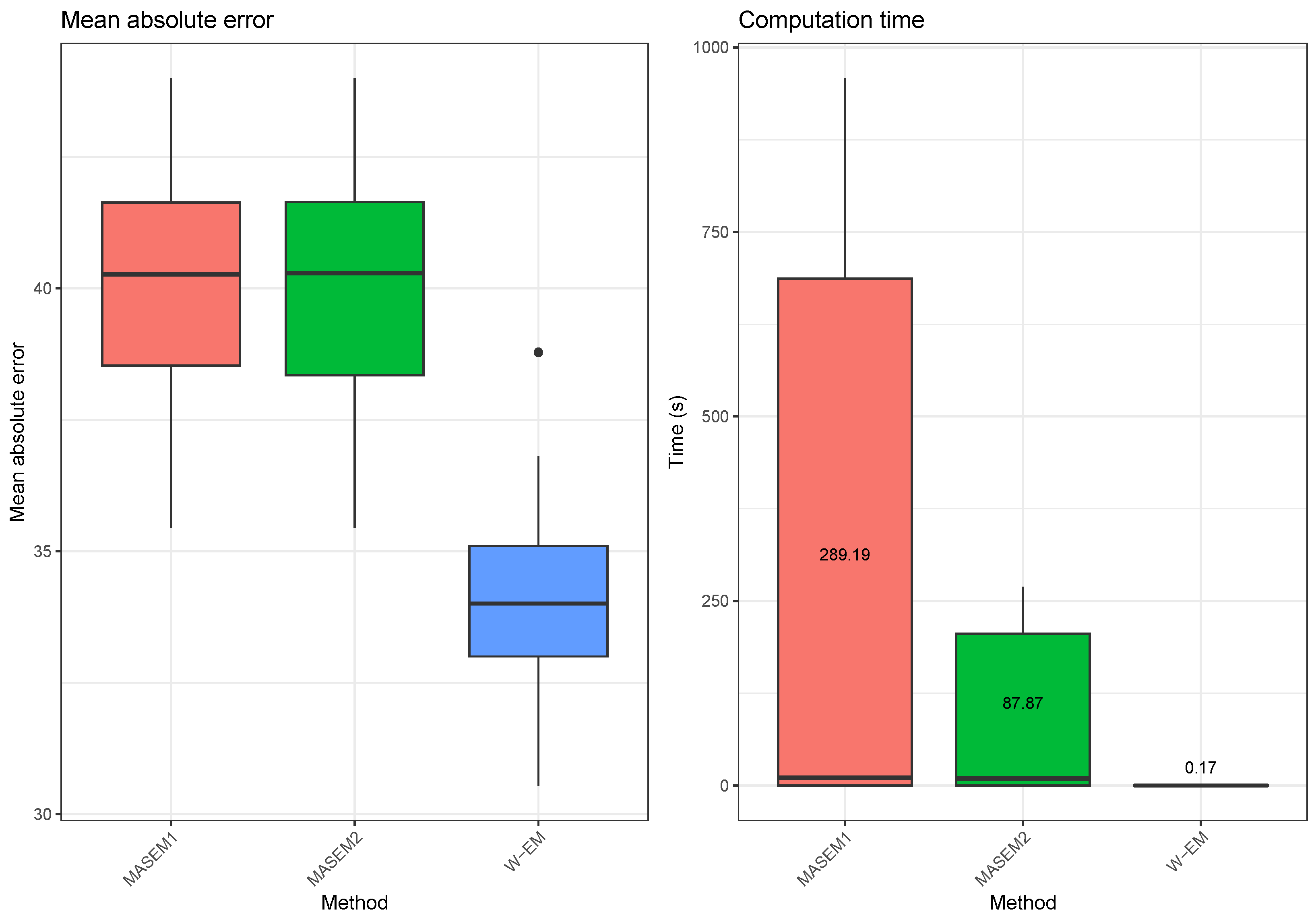
Illustration 3—Simulation study: Comparing the performance with MASEM

In this example, we compare our EM-based approach with the correlation pooling methods from the multivariate MASEM approach. We use the ”tssem1” function contained within the ”metaSEM” [33] R package for pooling covariance matrices using the MASEM approach. We use two different options for the random error structure in the MASEM approach: a diagonal error covariance matrix or a zero covariance matrix (since the variance component of the random effects is zero, the model becomes a fixed-effects model that is equivalent to the Generalized Least Squares (GLS) approach proposed by Becker [34]). When applying our method, we use the correlation matrices as covariance matrices, and before comparing it with the true parameter, we convert this matrix into a correlation matrix. The results are obtained by repeating the following simulation scenario 10 times. A random correlation matrix for 20 variables is generated. Using the random covariance matrix as the covariance parameter of a Wishart distribution with 100 degrees of freedom, we have generated three random covariance matrices. The first of these matrices contained the variables from 1 to 8, the second covariance matrix contained the variables 6 to 15 and the third matrix contained the variables 13 to 20. We have used our method as well as three forms of the MASEM approaches to obtain a complete covariance matrix estimate. We then compared the mean absolute error between the predicted and the true covariance matrix. The results, which are summarized in Figure 3, show that the EM-Algorithm for the Wishart distribution performs much better than the MASEM approaches in terms of the mean absolute errors and especially in terms of computation time. We also note that we could not make the MASEM algorithms produce any results for cases where the number of variables in the covariance matrix was larger than 30 in a reasonable time. This is due to the fact that the MASEM algorithms use a direct numerical optimization of the likelihood function, which becomes very difficult for unstructured covariance matrices. The EM-Algorithm for the Wishart distribution does not have this problem since each iteration of the algorithm depends solely on matrix algebra operations. More importantly, both of the MASEM approaches we have tried resulted in the imputation of previously unobserved correlation values with the same estimated common covariance parameter value.

Illustration 4—Empirical study: Cassava data

The need to exploit genomic and statistical tools to harness the total effects of all the genes in the crop genome is gaining traction in most crops. In our illustrations, we used the world’s largest and most updated public database for cassava (CassavaBase) from the Nextgen cassava funded project (http://www.nextgencassava.org). It is estimated that close to a billion people depend on cassava for their dietary needs, particularly in tropical regions of the world. We have accessed the data on 16 November 2019.

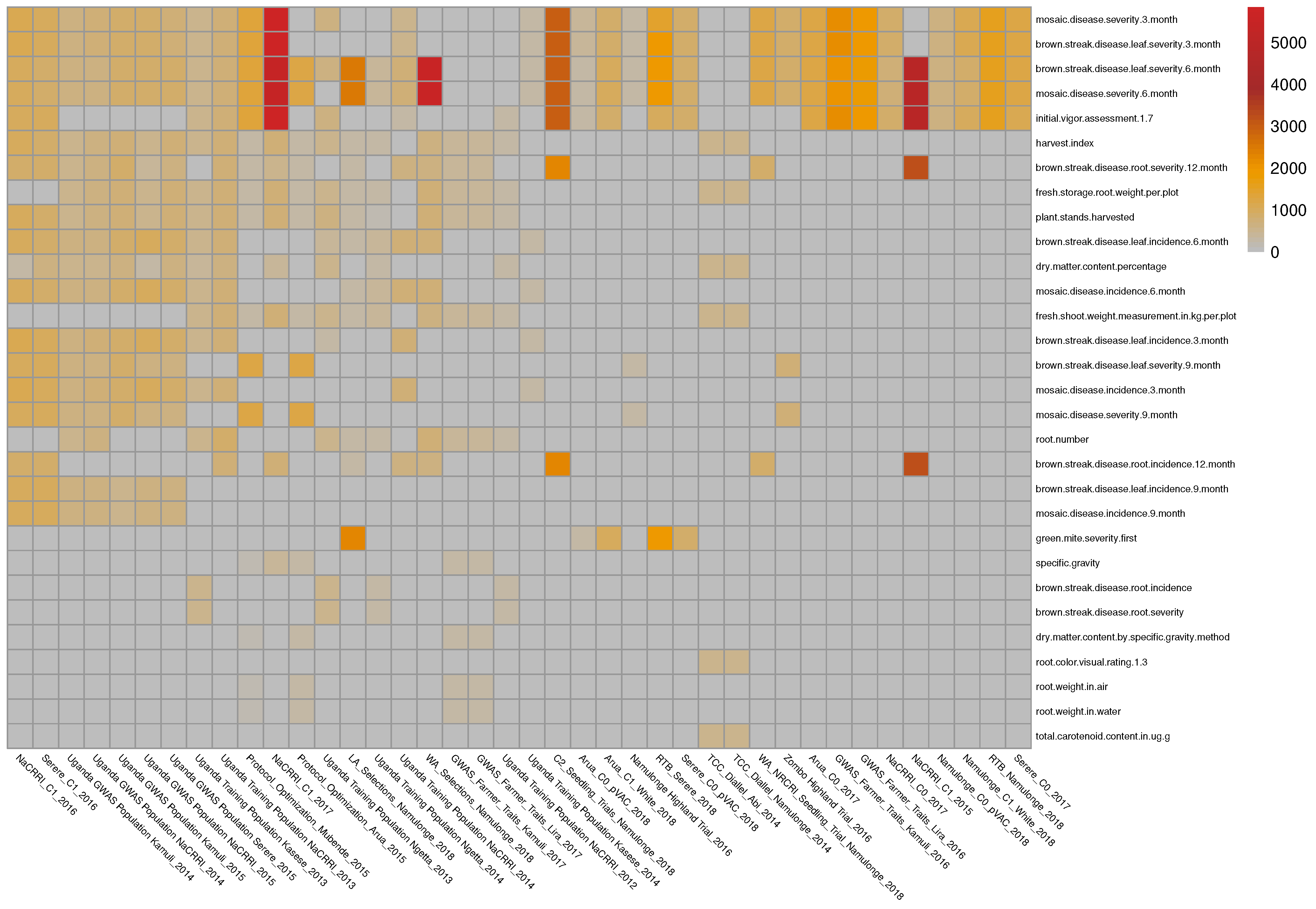
The initial data come from 135 phenotypic experiments performed by the East Africa cassava plant breeding programs. The dataset covers 81 traits and contains more than half a million phenotypic records. After filtering the outlier trait values, filtering the traits based on the number of records (at least 200 records per experiment), and trait–trial combinations also based on the number of records (at least 200 records for each trait in a given trial), a subset of 50 of these trials and a total of 37 traits were identified and used for this application (See Figure 4).

Due to the relatively high cost of phenotypic experiments, they typically focus on a limited set of key traits. As a result, when observing multiple phenotypic datasets, the data is typically heterogeneous and incomplete, with certain trait combinations not appearing together in any of the experiments (e.g., root weight in water and dry matter content percentage, root number and total carotenoid content).

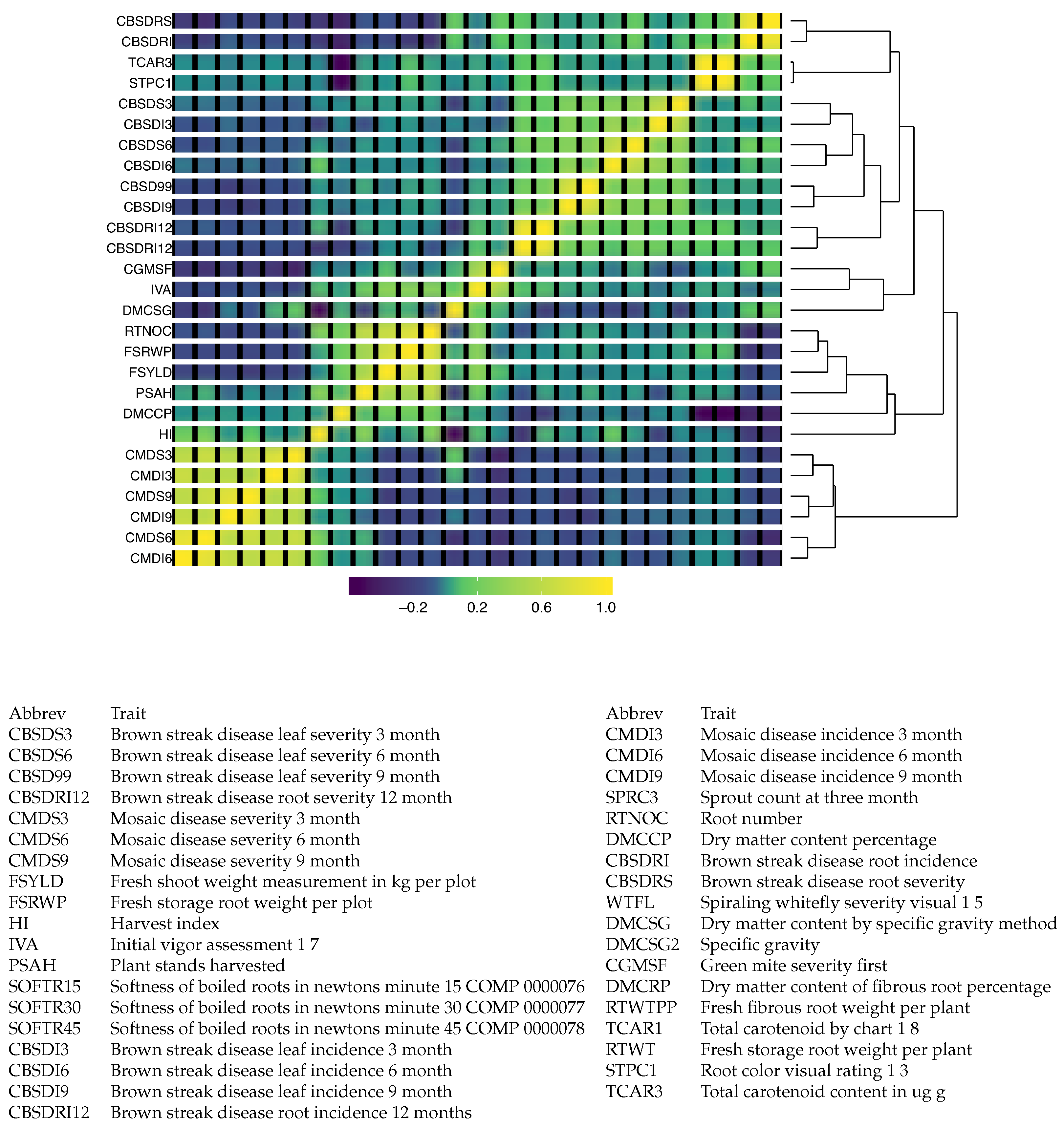
Figure 5 includes a heatmap of the resulting covariance matrix for 37 traits was obtained from combining the sample covariance matrices from 50 phenotypic trials. The heatmap indicates that there are three clusters of traits that appear to be positively correlated within each group, but little to no correlation between the groups. Two of these clusters correspond to disease-related traits, and the other is composed primarily of agronomic traits related to yield. The cluster related to cassava mosaic disease is found to be negatively correlated with the other disease traits, which are related to brown streak disease.

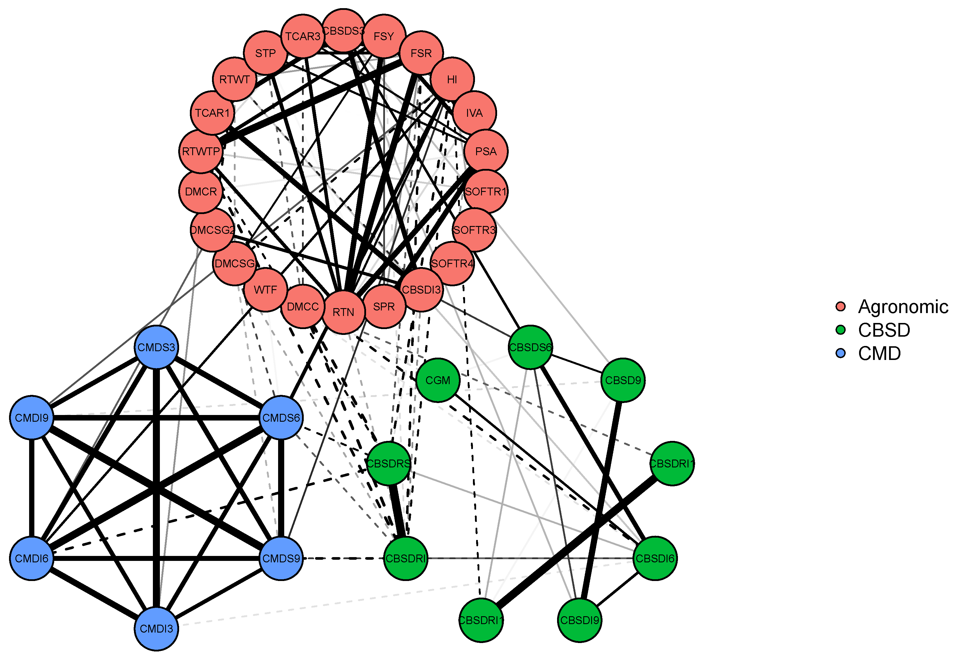
We have used the R Package qgraph [35] to introduce sparsity to the off-diagonal elements of the estimated covariance matrix and graphically present this in Figure 6.

4. Conclusions

Analyzing data in large and heterogeneous databases remains a challenge due to the need for new statistical methodologies and tools to make inferences. The EM-Algorithm for the Wishart distribution is one such tool that can be used to solve a very specific problem: combining datasets using covariance matrices (similarly combining relationship or similarity matrices). Our approach is highly beneficial in terms of its statistical formalism and computational efficiency; to the best of our knowledge, this is the first time the EM procedure for pooling covariance matrices has been described, although it has been inspired by similar methods such as (conditional) iterative proportional fitting for the Gaussian distribution [22,23] and a method for combining a pedigree relationship matrix and a genotypic relationship matrix, which includes a subset of genotypes from the pedigree-based matrix [24] (namely, the H-matrix).

Despite the benefits of the proposed framework for combining heterogeneous datasets, certain limitations should be taken into account. Specifically, when combining data using covariance matrices, the original features are not imputed. It is known that the nature of missingness in data can significantly influence the performance of imputation and inference. Consequently, any approaches that disregard the missing data mechanisms are only applicable to data that is missing completely at random (MCAR) or missing at random (MAR). However, such techniques cannot be utilized for data not missing at random (NMAR) [36,37]. Additionally, there could be heterogeneity in covariance matrices to some extent. This can be addressed with a hierarchical distribution (see, e.g., [38]). Furthermore, this structural misspecification can also be accounted for by the method in [39].

Overall, the combination of heterogeneous datasets via covariances matrices and the EM-Algorithm for the Wishart distribution is novel, and we expect it to be beneficial in a variety of fields, such as physics, engineering, biology, neuroscience, finance, genomics, and other -omics disciplines.