Novel Frequency-Based Approach to Analyze the Stability of Polynomial Fractional Differential Equations

Abstract

This paper proposes a novel approach for analyzing the stability of polynomial fractional-order systems using the frequency-distributed fractional integrator model. There are two types of frequency and temporal stabilization methods for fractional-order systems that global and semi-global stability conditions attain using the sum-of-squares (SOS) method. Substantiation conditions of global and asymptotical stability are complicated for fractional polynomial systems. According to recent studies on nonlinear fractional-order systems, this paper concentrates on polynomial fractional-order systems with any degree of nonlinearity. Global stability conditions are obtained for polynomial fractional-order systems (PFD) via the sum-of-squares approach and the frequency technique employed. This method can be effective in nonlinear systems where the linear matrix inequality (LMI) approach is incapable of response. This paper proposes to solve non-convex SOS-designed equations and design framework key ideas to avoid conservative problems. A Lyapunov polynomial function is determined to address the problem of PFD stabilization conditions and stability established using sufficiently expressed conditions. The main goal of this article is to present an analytical method based on the optimization method for fractional order models in the form of frequency response. This method can convert it into an optimization problem, and by changing the solution of the optimization problem, the stability of the fractional-order system can be improved.

1. Introduction

Fraction calculus has extensive applications in the field of engineering and modeling of physical processes, and for systems demanding perfect modeling]. In recent years, various systems have been developed using this approach through different numerical and mathematical techniques [1]. Moreover, numerous physical phenomena are controlled by fractional order equations; hence, more investigations and developments of these systems are required. One of the fundamental obstacles in the theory of fractional-order equations are the stability problems, so this issue has attracted a great deal of attention. Stability methods are classified into two significant categories: (i) the frequency method (a generalization of the Routh–Hurwitz technique [2] and (ii) the temporal method (a generalization of the Lyapunov technique) [3].

Taking advantage of the Lyapunov techniques is a prevailing method in the stability analysis of systems [4]. The first study on the stability of linear fractional-order systems (FOSs) was performed by Matignon [5]. Additionally, since then, the majority of researchers have investigated the stability of fractional-order systems. For example, Li et al. [6] reviewed the asymptotic stability and Mittage-Leffler stability of FOSs. Stability analysis of linear FOSs by the Lyapunov method and the linear matrix inequality approach (LMI) is presented in [7]. They examined the necessary and sufficient stability conditions and control state feedback designs. Two approaches for the Lyapunov stability for FOSs have been recommended: a direct approach that begets a parametric problem with a high dimension and an indirect approach that exploits the frequency model. The LMI method performs the stability analysis and gives a quick solution in an indirect approach [8].

In nonlinear FOSs, stability analysis is also highly complicated and there are fewer stabilization approaches. The direct Lyapunov technique is a specified method for the stability of nonlinear FOSs. Mittage-Leffler proposed the stability of nonlinear fractional-order systems adopting the direct method [9] and stated two stability theorems relative to fractional nonlinear time-delay systems [10]. Additionally, in this work [11], the Lyapunov method is used directly for stability analysis. In [12], the stability analysis of large-scale FOSs was surveyed then the system stability was investigated utilizing the indirect Lyapunov method, and the sufficient conditions were obtained for stability by applying the LMI inequality. The authors in [13] demonstrated that for equilibrium asymptotic stability, it is enough that the linearization system at equilibrium is asymptotically stable. Another method used for the stability analysis of FOSs is the distributed frequency model. This method has been used to analyze the fractional derivatives based on obtaining a relation between integer-order and fractional-order systems [14]. Since it is very difficult to construct a positive definite function, as well as to calculate the fractional derivative, a novel property has recently been utilized for the Caputo derivative. According to this method for stabilization analysis of FOSs, first the fractional-order inequality is stabilized, and this inequality creates a high boundary for the fractional-order derivative and provides a second-order Lyapunov function. This inequality explicates that if a positive definite function is a Lyapunov function for the integer order system, it will also be a Lyapunov function for an FOS [15]. The approach outcomes are applied to a quadratic Lyapunov function in the stability analysis of FOSs. In some cases, this Lyapunov function cannot perform satisfactorily and higher-order Lyapunov functions should be applied. These results are quite significant and contribute a fundamental tool for the analysis and stability of polynomial FOSs with a higher-order Lyapunov function. In [16], the stability analysis of fractional-order time-delay systems was investigated. The proposed method is based on modifying the convex part of the Lyapunov–Krasovkii function, which is employed in the stability analysis of Caputo FOSs with a range of (0, 1).

The main advantages of the proposed method lie in the following. In papers [16,17,18], a quadratic Lyapunov function was employed for stability analysis and conservative conditions were established. In this work, higher-degree Lyapunov functions have been adopted, and a wider range is checked for obtaining the Lyapunov function. The work by [19] studied fractional systems with specific characteristics and systems consisting of two sections: (i) the constant parameter matrix and (ii) the nonlinear function vector. This work has investigated the condition of stability for any class of nonlinear systems with unspecific characteristics.

When compared with the existing works for the stability analysis of nonlinear fractional differential systems [20,21,22], the LMI conditions were studied and this approach may not be practical in all situations, since there is a large number of nonlinear systems that cannot be represented in terms of LMIs. In this paper, the SOS condition is proposed and the stability of many nonlinear systems can be examined in this way.

Notation:

In this work, we will consider the following notations:

$R^n$ denotes the n-dimensional Euclidean space and $A^{*}=\overline{A^T}={\overline{A}}^T$;

$A^{*}$ denotes for the transpose conjugate, $A^T$ denotes the transpose and $\overline{A}$ is the conjugate of matrix A;

Matrix $A^{†}$ denotes the generalized inverse of matrix A which satisfies $A{A}^{†}A=A$ and $ran\left(A\right)=A{A}^{†}$.

2. Principle

This section is dedicated to briefly recalling a framework of fractional calculus and the explicit solution of the operator equation.

Definition 1

[17]. The Caputo fractional derivative is defined as follows:

$${ }_{t_0}^c{D}_t^{q}f\left(t\right)=\frac{1}{\mathsf{\Gamma }\left(n-q\right)}{{\displaystyle \int }}_{t_0}^t{\left(t-\tau \right)}^{n-q-1}{f}^{\left(n\right)}\left(\tau \right)d\tau$$

(1)

where q is the fractional order, $n$ − 1 ≤ $q$ < $n$. $\Gamma \left(·\right)$ represents the Euler’s function and $\Gamma \left(t\right)={\int }_0^{\infty }{x}^{t-1}{e}^{-x}dx$.

Lemma 1

[23]. Let $x_1\in B\left(H\right)$ closed range and $x_2\in B\left(K,H\right)$ and $x_3\in B\left(K,H\right)$ and $x_4\in B\left(K,H\right)$. $H,K$ and $L$ denote complex Hilbert space and $B\left(K,H\right)$ is the set of all bounded linear operator between $H$ and $K$.

Assume that $=\left(\begin{array}{ll}{x}_1\hfill & x_2\hfill \\ x_3\hfill & x_4\hfill \\ \hfill & \hfill \end{array}\right)$.

$P$ is positive if and only if

• $x_1=x_1^{*},x_4=x_4^{*},x_3=x_2^{*}$;
• $x_1{x}_1^{†}{x}_2=x_2$;
• $x_4-x_3{x}_1^{†}{x}_2\in L{(x)}_{+}$.

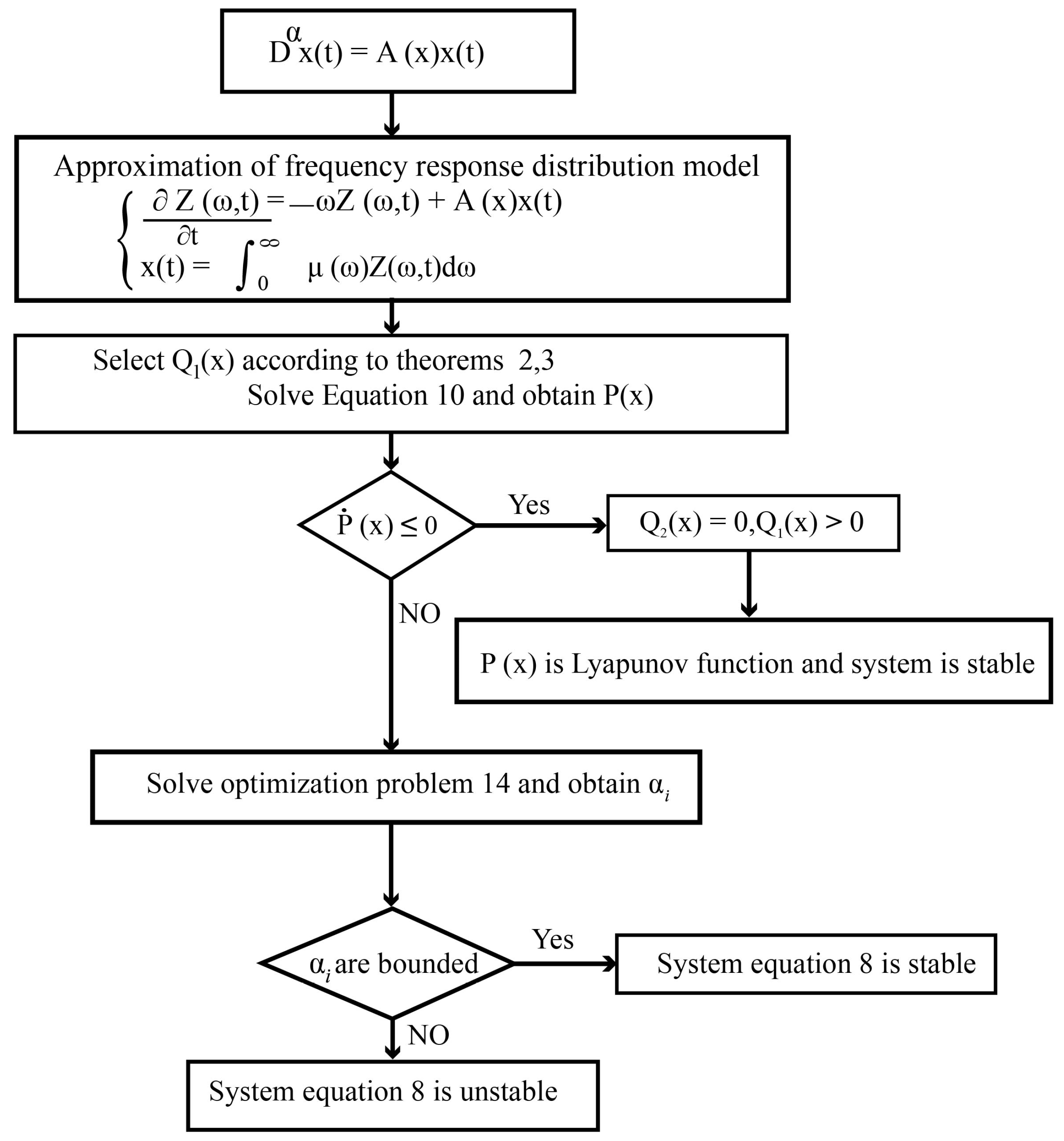
The Positive Solutions for Operator Equation $A^{T}X+XA=B$

Consider the equation:

$$A^{T}X+XA=B$$

(2)

Theorem 1.

Let $X$ be a Hilbert A-module and $A,B\in L\left(x\right)$. Suppose that $BA$ are closed ranges and $BA$ is a positive operator, $B{B}^{†}=\left(BA\right){(BA)}^{†}$ and $(1-\left(A^T{)}^{†}{A}^T\right)B^{†}=0$, then equation $A^{T}X+XA=\mathrm{B}$ has a particular positive solution $X\in L{(X)}_{+}$ if and only if B is self-adjoint and

$$(1-A^T\left(A^T{)}^{†}\right)B(1-A^T\left(A^T{)}^{†}\right)=0.$$

The particular positive solution has the form $X=\frac{1}{2}{B}^T{(BA)}^{†}$.

Proof. 

Suppose that equation $A^{T}X+XA=B$ has a solution $X\in ℒ{(\mathcal{X})}_{+}$. Obviously, $B=B^{*}$. Additionally, we have

$$\begin{array}{}(1-A^T\left(A^T{)}^{†}\right)B(1-A^T\left(A^T{)}^{†}\right)=(1-A^T\left(A^T{)}^{†}\right)\left(A^{T}X+X^{*}A\right)(1-A^T\left(A^T{)}^{†}\right)\\ =(1-A^T\left(A^T{)}^{†}\right)A^{T}X(1-A^T\left(A^T{)}^{†}\right)+(1-A^T\left(A^T{)}^{†}\right)X^{*}A(1-A^T\left(A^T{)}^{†}\right)\\ =0.\end{array}$$

Conversely, assume that $B$ is self-adjoint and $(1-A^T\left(A^T{)}^{†}\right)B(1-A^T\left(A^T{)}^{†}\right)=0$. Take $P_1=B^{†}B$, $P_2=1-B^{†}B$ and $X_1=P_{1}X{P}_1$. From the assumption $(1-\left(A^T{)}^{†}{A}^T\right)B^{†}=0$, we obtain

$$X_1=P_{1}X{P}_1=B^{†}BX{B}^{†}B=\frac{1}{2}{B}^{*}{(BA)}^{†}B$$

and hence $BA\in ℒ{(\mathcal{X})}_{+}$ implies that $X_1\in ℒ{(\mathcal{X})}_{+}$. Moreover, since $\mathrm{ran}\left(B\right)=\mathrm{ran}\left(BA\right)$, we obtain

$$\begin{array}{ll}{X}_1(2B^{†}\left(BA\right)\left(B^{*}{)}^{†}\right)X_1& =\frac{1}{2}{B}^{*}{(BA)}^{†}B(B^{†}\left(BA\right)\left(B^{*}{)}^{†}\right)B^{*}{(BA)}^{†}B\\ & =\frac{1}{2}{B}^{*}{(BA)}^{†}B{B}^{†}\left(BA\right)B{B}^{†}{(BA)}^{†}B\\ & =\frac{1}{2}{B}^{*}{(BA)}^{†}B,\end{array}$$

Thus, $X_1$ is regular and $X_1^{†}=B^{†}\left(BA\right){(B^{*})}^{†}$. We can write

$$X=X_1+X_2+X_3+X_4=P_{1}X{P}_1+P_{1}X{P}_2+P_{2}X{P}_1+P_{2}X{P}_2,$$

where

$$X_2=P_{1}X{P}_2=B^{†}BX\left(1-B^{†}B\right)=B^{*}{(BA)}^{†}BV(1-\left(A^T{)}^{†}{A}^T\right),$$

$$X_3=P_{2}X{P}_1=\left(1-B^{†}B\right)X{B}^{†}B=(1-\left(A^T{)}^{†}{A}^T\right)V^{*}{B}^{*}{(BA)}^{†}B,$$

$$\begin{array}{ll}{X}_4=P_{2}X{P}_2& =\left(1-B^{†}B\right)X\left(1-B^{†}B\right)\\ & =2(1-\left(A^T{)}^{†}{A}^T\right)V^{*}{B}^{*}{(BA)}^{†}BV(1-\left(A^T{)}^{†}{A}^T\right)+(1-\left(A^T{)}^{†}{A}^T\right)W(1-\left(A^T{)}^{†}{A}^T\right).\end{array}$$

Evidently, $X_3=X_2^{*}$ and $X_1{X}_1^{†}{X}_2=X_2$. Furthermore, we have

$$\begin{array}{}{X}_4-X_3{X}_1^{†}{X}_2=2(1-\left(A^T{)}^{†}{A}^T\right)V^{*}{B}^{*}{(BA)}^{†}BV(1-\left(A^T{)}^{†}{A}^T\right)+\\ (1-\left(A^T{)}^{†}{A}^T\right)W(1-\left(A^T{)}^{†}{A}^T\right)\\ -((1-\left(A^T{)}^{†}{A}^T\right)V^{*}{B}^{*}\left(BA{)}^{†}B\right)(B^{†}\left(BA\right)\left(B^{*}{)}^{†}\right)(2B^{*}{(BA)}^{†}BV(1-\left(A^T{)}^{†}{A}^T\right)\\ =(1-\left(A^T{)}^{†}{A}^T\right)W(1-\left(A^T{)}^{†}{A}^T\right)\in ℒ{(\mathcal{X})}_{+}\end{array}$$

(3)

Applying Lemma 1, we derive that $X$ is positive. □

Theorem 2.

The negative solution of operator equation $A^{T}P+PA=-Q$.

Consider the equation:

$$A^{T}P+PA=-Q$$

(4)

$A,P,Q\in L\left(X\right),Q$, according to Lemma 2, is positive and $\left(-Q\right)A^T$ is negative:

$$\left(-Q\right){(-Q)}^{†}=\left(QA\right){(QA)}^{†}$$

Applying Theorem 2, Equation (4) then has a negative solution.

$$P=\frac{1}{2}\left(-Q^T\right){(-Q{A}^T)}^{†}\left(-Q\right).$$

(5)

3. Main Theorem

In this section, sufficient conditions are derived for the asymptotical stability of the polynomial fractional differential equations system in terms of the sum-of-squares (SOS) approach. In this section, we have established a Lyapunov candidate function for a fractional-order system to analyze the asymptotic behavior around the equilibrium points. Heleschewitz and Matignon [21] and Laudebat [22] proposed the diffusive representation that provides the theoretical equations which can be expressed as follows:

Let us consider a linear system such as

$$y\left(t\right)=h\left(t\right)\ast v_0\left(t\right) , h\left(t\right)={{\displaystyle \int }}_0^{\infty }\mu \left(\omega \right)e^{-\omega t}d\omega$$

(6)

where $h\left(t\right)$ is the impulse response of the linear system and $\mu \left(\omega \right)$ is a diffusive representation of impulse response; $h\left(t\right)$ verifies the pseudo-Laplace transform.

$\mu \left(\omega \right)$ has the following form:

$$\mu \left(\omega \right)=\frac{\sin \left(q\pi \right)}{\pi }{\omega }^{-q}.$$

(7)

Consider a polynomial fractional differential equation system:

$$D^{q}x\left(t\right)=A\left(x\right)x\left(t\right)$$

(8)

where $A\left(x\right)\in {ℝ}^{n\times n}$ is a polynomial nonlinear system matrix, $x\left(t\right)\in {ℝ}^n$ is the system state vector, and $q$ is the fractional-order derivative with 0 <$q$< 1.

By using the continuous frequency distributed model of the fractional integrator, System (8) can be expressed [9] as follows:

$$\{\begin{array}{ll}\frac{\partial Z\left(\omega ,t\right)}{\partial t}=-\omega Z\left(\omega ,t\right)+v_0\left(t\right)=-\omega Z\left(\omega ,t\right)+A\left(x\right)x\left(t\right).\hfill & \hfill \\ x\left(t\right)={{\displaystyle \int }}_0^{\infty }\mu \left(\omega \right)Z\left(\omega ,t\right)d\omega .\hfill & \hfill \end{array}$$

(9)

Theorem 3.

The sufficient condition for the asymptotic stability of the polynomial FOS given in Equation (9) indicates that positive definite matrixes $Q_1\left(x\right)$, $P\left(x\right)$> 0, and polynomials $q_2\left(x\right)$ result in the following relations being established:

The polynomial fractional-order system given in Equation (9) is asymptotic stability if and only if definite matrixes $Q_1\left(x\right)$, $P\left(x\right)$> 0, and polynomials $q_2\left(x\right)$ exist such that the following conditions hold.

$$A^T\left(x\right)P\left(x\right)+P\left(x\right)A\left(x\right)=-Q_1\left(x\right).$$

(10)

$${{\displaystyle \int }}_0^{\infty }\mu \left(\omega \right)Z^T\left(\omega ,t\right)\left( \dot{P}\left(x\right)-2\omega P\left(x\right)\right)Z\left(\omega ,t\right)d\omega <q_2\left(x\right).$$

(11)

$$q_2\left(x\right)-x^T{Q}_1\left(x\right)x\le 0.$$

(12)

$$Q_1\left(x\right),P\left(x\right)>0.$$

(13)

Proof: 

Consider the monochromatic Lyapunov function $v\left(\omega ,t\right)$ which leads to the PFDE Lyapunov function $V\left(t\right)$:

$$v\left(\omega ,t\right)=Z^T\left(\omega ,t\right)P\left(x\right)Z\left(\omega ,t\right), P\left(x\right)>0$$

$V\left(t\right)$ is the Lyapunov function summing all the mono-chromatic $v\left(\omega ,t\right)$ with the weighting function $\mu \left(\omega \right)$:

$$V\left(t\right)={{\displaystyle \int }}_0^{\infty }\mu \left(\omega \right)v\left(\omega ,t\right)d\omega ={{\displaystyle \int }}_0^{\infty }\mu \left(\omega \right)Z^T\left(\omega ,t\right)P\left(x\right)Z\left(\omega ,t\right)d\omega$$

By calculating the derivative of the above Lyapunov function using Equation (9), we obtain

$$\begin{array}{ll}\dot{V}\left(t\right)& ={{\displaystyle \int }}_0^{\infty }\mu \left(\omega \right)\frac{\partial }{\partial t}\left[Z^T\left(\omega ,t\right)P\left(x\right)Z\left(\omega ,t\right)\right]d\omega \\ & ={{\displaystyle \int }}_0^{\infty }\mu \left(\omega \right)\left[ \frac{\partial }{\partial t}{Z}^T\left(\omega ,t\right)P\left(x\right)Z\left(\omega ,t\right)+Z^T\left(\omega ,t\right)\frac{\mathrm{d}P\left(x\right)}{\mathrm{d}t}Z\left(\omega ,t\right)+Z^T\left(\omega ,t\right)P\left(x\right)\frac{\partial Z\left(\omega ,t\right)}{\partial t}\right]d\omega \\ & ={{\displaystyle \int }}_0^{\infty }\mu \left(\omega \right)\left[{\left(-\omega Z\left(\omega ,t\right)+A\left(x\right)x\left(t\right)\right)}^{T}P\left(x\right)Z\left(\omega ,t\right)+Z^T\left(\omega ,t\right)\dot{P}\left(x\right)Z\left(\omega ,t\right)+Z^T\left(\omega ,t\right)P\left(x\right)\left(-\omega Z\left(\omega ,t\right)+A\left(x\right)x\left(t\right)\right)\right]d\omega \\ & =-2{{\displaystyle \int }}_0^{\infty }\omega \mu \left(\omega \right)Z^T\left(\omega ,t\right)P\left(x\right)Z\left(\omega ,t\right)d\omega \\ & +{{\displaystyle \int }}_0^{\infty }\mu \left(\omega \right){[A\left(x\right)x\left(t\right)]}^{T}P\left(x\right)Z\left(\omega ,t\right)d\omega \\ & +{{\displaystyle \int }}_0^{\infty }\mu \left(\omega \right)\left[Z^T\left(\omega ,t\right)P\left(x\right)A\left(x\right)x\left(t\right)\right]d\omega \\ & +{{\displaystyle \int }}_0^{\infty }\mu \left(\omega \right)Z{(\omega ,t)}^T\dot{P}\left(x\right)Z\left(\omega ,t\right)d\omega \\ & =-2{{\displaystyle \int }}_0^{\infty }\omega \mu \left(\omega \right)\left[Z^T\left(\omega ,t\right)P\left(x\right)Z\left(\omega ,t\right)\right]d\omega \\ & +{(A\left(x\right)x\left(t\right))}^{T}P\left(x\right){{\displaystyle \int }}_0^{\infty }\mu \left(\omega \right)Z\left(\omega ,t\right)d\omega \\ & +{{\displaystyle \int }}_0^{\infty }\omega \mu \left(\omega \right)\left[Z^T\left(\omega ,t\right)d\omega \right)P\left(x\right)A\left(x\right)x\left(t\right)\\ & +{{\displaystyle \int }}_0^{\infty }\mu \left(\omega \right)Z{(\omega ,t)}^T\dot{P}\left(x\right)Z\left(\omega ,t\right)d\omega \\ & =-2{{\displaystyle \int }}_0^{\infty }\omega \mu \left(\omega \right)\left[Z^T\left(\omega ,t\right)P\left(x\right)Z\left(\omega ,t\right)\right]d\omega +x^T\left(t\right)\left[A^T\left(x\right)P\left(x\right)+P\left(x\right)A\left(x\right)\right]x\left(t\right)\\ & +{{\displaystyle \int }}_0^{\infty }\mu \left(\omega \right)Z^T\left(\omega ,t\right)\dot{P}\left(x\right)Z\left(\omega ,t\right)d\omega \\ & =x^T\left(t\right)\left[A^T\left(x\right)P\left(x\right)+P\left(x\right)A\left(x\right)\right]x\left(t\right)\\ & +{{\displaystyle \int }}_0^{\infty }\mu \left(\omega \right)Z^T\left(\omega ,t\right)\left(\dot{P}\left(x\right)-2\omega P\left(x\right)\right)Z\left(\omega ,t\right)d\omega \end{array}$$

Therefore, according to the assumptions of the theorem, we obtain

$$\dot{V}\left(t\right)\le -x^T\left(t\right)Q_1\left(x\right)x\left(t\right)+q_2\left(x\right)<0$$

where $\dot{P}\left(x\right)$ is stated as follows:

$$\dot{P}\left(x\right)={\left[{\sum }_{k=1}^n\frac{\partial P_{i,j}\left(x\right)}{\partial x_k}\frac{d{x}_k}{dt}\right]}_{i,j}$$

□

Notation 1:

In the particular case $q_2\left(x\right)=x^T{Q}_1\left(x\right)x$ can be satisfied.

Notation 2:

By defining the matrix $Q_2 \left(x\right)$ so that $q_2\left(x\right)=x^T{Q}_2\left(x\right)x$, the conditions of the theorem can be converted as follows: $Q_1\left(x\right),P\left(x\right)>0$ and $Q_2\left(x\right)-Q_1\left(x\right)\le 0$, where $Q_2\left(x\right)$ is indefinite.

Notation 3:

If $\dot{P}\left(x\right)\le 0$, the answer to the problem can be settled by selecting $Q_2\left(x\right)=0,Q_1 \left(x\right)>0$ and only by solving Equation (10).

By selecting the appropriate value for m, such that

$$\mathrm{deg}\left(x^T{Q}_2\left(x\right)x\right)\le \mathrm{deg}\left(x^T{Q}_1\left(x\right)x\right)$$

To specify the $Q_2\left(x\right)$ matrix, consider the following optimization problem:

$$\begin{array}{}\mathrm{Min} \mathrm{J}\left({\alpha }_0,{\alpha }_1,\cdots ,{\alpha }_m\right)={\alpha }_0+{\alpha }_1+\frac{1}{2}{\alpha }_2+\cdots +\frac{1}{m}{\alpha }_m\\ subject to:\\ {{\displaystyle \int }}_0^{\infty }\mu \left(\omega \right)Z^T\left(\omega ,t\right)\left( \dot{P}\left(x\right)-2\omega P\left(x\right)\right)Z\left(\omega ,t\right)d\omega \le x^T{Q}_2\left(x\right)x\\ A^T\left(x\right)P\left(x\right)+P\left(x\right)A\left(x\right)=-Q_1\left(x\right)\end{array}$$

(14)

$$\begin{array}{}{{\displaystyle \int }}_0^{\infty }\mu \left(\omega \right)Z\left(\omega ,t\right)d\omega =x\left(t\right)\\ Q_2\left(x\right)={\alpha }_0{I}_n+{\alpha }_1{x}^{T}x{I}_n+\cdots +{\alpha }_m{\left(x^{T}x\right)}^m{I}_n\\ Q_2\left(x\right)-Q_1\left(x\right)\le 0\\ Q_1\left(x\right),P\left(x\right)>0\\ {\alpha }_i\in ℝ, i=1,2,3,\cdots ,m\end{array}$$

Notation 4:

The objective function of the optimization Problem (14) is such that the values ${\alpha }_i$ lessen with increasing $i$ to ascertain the matrix $Q_2\left(x\right)$ Therefore, $Q_2\left(x\right)$ is defined in the simplest format.

Notation 5:

Various formats can be considered for the $Q_2\left(x\right)$ matrix. This paper takes into account a simple diagonal form. In general, and in the optimization Problem (14), $Q_2\left(x\right)$ can be described as follows:

$$Q_2\left(x\right)={\alpha }_0{D}_0+{\alpha }_1\left(x^T.x\right)D_1+\cdots +{\alpha }_m{\left(x^T.x\right)}^m{D}_m={\displaystyle \sum }_{i=0}^m{\alpha }_i{\left(x^T.x\right)}^i{D}_i$$

where $D_i\in {ℝ}^{n\times n} , i=1,2,\cdots m$ are arbitrary positive definite matrixes.

Since $\left(\dot{P}\left(x\right)-2\omega P\left(x\right)\right)$ is an indefinite, the matrix $Q_2\left(x\right)$ is also indefinite, which is related to the value of the coefficients ${\alpha }_i$. If all of the coefficients ${\alpha }_i$ are positive (negative), then $Q_2\left(x\right)$ is definitely positive (definitely negative), otherwise $Q_2\left(x\right)$ is indefinite. By solving the above optimization problem, the values of ${\alpha }_i$ and, consequently, matrix $Q_2\left(x\right)$, are achieved. A remarkable point is that if the answer to the above problem is not bounded, it implies that $\Vert Z\left(\omega ,t\right)\Vert or \Vert x\left(t\right)\Vert$ are not bounded, which is equivalent to system instability. Therefore, a stable system ${\alpha }_i$ is bounded and, as a result, $Q_2\left(x\right)$ is determined.

Theorem 4:

A sufficient condition for the stability of the polynomial FOS (9) is that the optimization Problem (14) has a bounded answer.

Proof: 

Similar to Theorem 3. □

Notation 6:

$\dot{P}\left(\mathrm{x}\right)$ can be computed as follows:

$$\dot{P}\left(x\right)={\left[{\displaystyle \sum }_k\frac{\partial P_{i,j}\left(x\right)}{\partial x_k}\frac{d{x}_k}{dt}\right]}_{i,j}={\left[{\displaystyle \sum }_k\frac{\partial P_{i,j}\left(x\right)}{\partial x_k}{{\displaystyle \int }}_0^{\infty }\mu \left(\omega \right)\frac{\partial Z_k\left(\omega ,t\right)}{\partial t}d\omega \right]}_{i,j}$$

(15)

where $Z_k\left(\omega ,t\right)$ is the kth component of the vector $Z\left(\omega ,t\right)$, and $x_k$ is the kth component of the $x\left(t\right)$ vector.

By employing the approximation of the frequency response distribution model, integral constraints can be converted into algebraic and linear relations:

This continuous frequency distributed model in Theorem 3 is not directly usable. Hence, the function μ(ω) is replaced by a multiple-step function μ(${\omega }_k$). Thus, the continuous distributed model becomes a conventional state model expressed in Equation (16). Consider a finite network of j frequency points, $\omega =\left[{\omega }_1\dots \dots {\omega }_j\right]$, where j is the number of approximation nodes.

$$\mathrm{x}\left(t\right)={\displaystyle \sum }_{\mathrm{k}=1}^{\mathrm{j}}\mu \left({\omega }_k\right)Z_{\mathrm{k}}\left(t\right)\mathsf{\Delta }\left({\omega }_k\right)={\displaystyle \sum }_{\mathrm{k}=1}^{\mathrm{j}}{\mathrm{c}}_{\mathrm{k}}{Z}_{\mathrm{k}}\left(t\right)$$

(16)

$\omega =\left[{\omega }_1\dots \dots {\omega }_j\right]$ where j is frequency points.

$$c_k=\mu \left({\omega }_k\right)\mathsf{\Delta }\left({\omega }_k\right)$$

(17)

$$\frac{{\mathrm{dz}}_{\mathrm{k}}\left(t\right)}{\mathrm{dt}}={\mathrm{A}}_1\underset{\_}{\mathrm{z}}\left(t\right)$$

(18)

The approximate value of the vector of $\mathrm{x}\left(t\right)$ is given as follows:

$$\underset{\_}{\mathrm{x}}\left(t\right)={\underset{\_}{{\mathrm{c}}_1}}^t\underset{\_}{\mathrm{z}}\left(t\right)$$

(19)

An approximate of the state $\mathrm{Z}\left(\omega ,t\right)$ is $\underset{\_}{\mathrm{z}}\left(t\right)$.

$$\underset{\_}{z}\left(t\right)=\left[\begin{array}{c}{Z}_1\\ .\\ .\\ .\\ Z_j\end{array}\right] \mathrm{and} A_1= \left(\begin{array}{ccc}-w1& & 0\\ & \ddots & \\ 0& & -wj\end{array}\right)$$

From Equation (16), we obtain

$${(c_1^T)}^{†}\underset{\_}{\mathrm{x}}\left(t\right)={(c_1^T)}^{†}{c}_1^T\underset{\_}{\mathrm{z}}\left(t\right)={(c_1^T)}^{†}\underset{\_}{\mathrm{x}}\left(t\right)=\underset{\_}{\mathrm{z}}\left(t\right)$$

(20)

To analyze and determine the answer to the optimization problem, the following can be fulfilled:

First, by selecting $Q_1\left(x\right)$ according to Theorems 1 and 2, $P\left(x\right)>0$ can be obtained by solving the equation $A^T\left(x\right)P\left(x\right)+P\left(x\right)A\left(x\right)=-Q_1\left(x\right)$

Then, for the function, the objective is defined and resolved by the resulting constraints, which are no longer integral but linear and dependent on the frequency value ${\omega }_k$, and finally, $Q_2\left(x\right)$ is settled.

4. Strengths and Future Research

In this paper, the method of stability analysis of nonlinear FOSs in the frequency domain is highlighted, then, instead of using LMI that leads to the Lyapunov function of degree 2, the technique SOS has been used, and the conditions for obtaining the function with more degrees have been provided; as a result, the volume of calculations has increased. The advantages and disadvantages of the proposed approach are as follows:

(1)

It provides a new perspective on the stability analysis of SOS-based FOSs;

(2)

It is possible to determine a higher-order Lyapunov function;

(3)

The fractional-order system’s stability can be obtained despite an optimization problem’s bounded solution.

The limitations of the proposed system are as follows:

(1)

High computational volume in resolving optimization problems;

(2)

Absence of uncertainty in the proposed method.

In this method, the fractional-order system model is converted into a frequency model and the Lyapunov function is obtained by solving Equation (10). By incorporating the derivative of the function p(x) and determining its sign and solving the optimization equation, the stability of the system is determined (Figure 1).

Example. 

Consider the following polynomial fractional differential equations system:

$$\begin{array}{ll}{}_{t_0}{}^{c}D{}_t^{0.8}{x}_1\left(t\right)& =-4x_1+2x_1{x}_2{}^2+x_2{}^2+x_1{}^2-2x_1{x}_2\\ {}_{t_0}{}^{c}D{}_t^{0.8}{x}_2\left(t\right)& =-x_2-2x_2{x}_1{}^2\\ A\left(x\right)& =\left[\begin{array}{cc}-4+x_1& 2x_1{x}_2+x_2-2x_1\\ -2x_1{x}_2& -1\end{array}\right]\end{array}$$

(21)

Select $Q_1\left(x\right)$ according to Theorems 2 and 3:

$$Q_1\left(x\right)=\left[\begin{array}{cc}{Q}_{1,1}& Q_{1,2}\\ Q_{2,1}& Q_{2,2}\end{array}\right]$$

$$\begin{array}{}{Q}_{1,1}=252x_1^2{x}_2^2+126x_1^2+78x_1{x}_2^3-4x_1{x}_2+136x_2^2+184\\ Q_{1,2}=Q_{2,1}=252x_1^3{x}_2+126x_1^2{x}_2^2+25.121x_1{x}_2^3+557x_1{x}_2-130x_2^4+242.83x_2^2-3\\ Q_{2,2}=210.42x_1^2{x}_2^2+252x_1^2+330x_1{x}_2^3-4x_1{x}_2+33.12x_2^4+2073.12x_2^2+368\end{array}$$

Obtain $P\left(x\right)$ by solving Equation (10):

$$P\left(x\right)=\left[\begin{array}{cc}0.63x_1^2+0.68x_2^2+0.92& 0.195x_2^2+0.63x_1{x}_2– 0.01\\ 0.195x_2^2+0.63x_1{x}_2-0.01& 0.63x_1^2+0.68x_2^2+0.92\end{array}\right]$$

By solving optimization Problem (14):

$${\alpha }_0=1.5646,{\alpha }_1=2.0378$$

$$Q_2\left(x\right)=\left[\begin{array}{cc}1.5646+2.0378\left(x_1^2+x_2^2\right)& 0\\ 0& 1.5646+2.0378\left(x_1^2+x_2^2\right)\end{array}\right]$$

$$Q_2\left(x\right)-Q_1\left(x\right)\le 0$$

Then, according to Theorem 3, System (21) is asymptotically stable.

In Figure 2, The phase portrait of the system is drawn for different initial conditions, which shows the stability of the system (21).The matrix $Q_2\left(x\right)$ is obtained by solving the optimization equation and determining ${\alpha }_0$,${\alpha }_1$. In Figure 3, it is shown that condition $Q_2\left(x\right)-Q_1\left(x\right)\le 0$ is satisfied by choosing $\mathrm{h}\left(x\right)=x^T\left(Q_2\left(x\right)-Q_1\left(x\right)\right)x\le 0$.

5. Conclusions

In this paper, the stability analysis of polynomial fractional-order systems is investigated. The direct method of the Lyapunov function is chosen, based on which, sufficient conditions for the stability of PFD systems are achieved. Using this approach, a higher-order Lyapunov function is extracted, and it is conceivable to survey systems with high nonlinearity degrees. This paper revealed that Equation (8), whose frequency’s equivalent is Equation (9), is globally stable if the optimization problem Equation (14) has a bounded solution. In addition, the stability study of FOSs has been broadened to systems that cannot be represented as LMIs. Lyapunov’s polynomial function is proposed based on the sum-of-squares approach for fractional-order systems. In the future, we intend to develop this system in the presence of uncertainty.

References

- Ortigueira, M.D. Fractional Calculus for Scientists and Engineers; Springer Science & Business Media: Berlin, Germany, 2011; Volume 84. [Google Scholar]
- Hurwitz, A. Ueber die Bedingungen, unter welchen eine Gleichung nur Wurzeln mit negativen reellen Theilen besitzt. Math. Ann. 1985, 46, 273–284. [Google Scholar] [CrossRef]
- Chen, W.; Dai, H.; Song, Y.; Zhang, Z. Convex Lyapunov functions for stability analysis of fractional order systems. IET Control. Theory Appl. 2017, 11, 1070–1074. [Google Scholar] [CrossRef]
- Benzaouia, A.; Hmamed, A.; Mesquine, F.; Benhayoun, M.; Tadeo, F. Stabilization of continuous-time fractional positive systems by using a Lyapunov function. IEEE Trans. Autom. Control. 2014, 59, 2203–2208. [Google Scholar] [CrossRef]
- Matignon, D. Stability results for fractional differential equations with applications to control processing. Comput. Eng. Syst. Appl. 1996, 2, 963–968. [Google Scholar]
- Li, Y.; Chen, Y.; Podlubny, I. Stability of fractional-order nonlinear dynamic systems: Lyapunov direct method and generalized Mittag–Leffler stability. Comput. Math. Appl. 2010, 59, 1810–1821. [Google Scholar] [CrossRef]
- Sabatier, J. On Stability and Performances of Fractional Order Systems. In Proceedings of the 3rd IFAC Symposium FDA’08, 2008, Ankara, Turkey.
- Trigeassou, J.C.; Maamri, N.; Sabatier, J.; Oustaloup, A. A Lyapunov approach to the stability of fractional differential equations. Signal Process. 2011, 91, 437–445. [Google Scholar] [CrossRef]
- Li, C.; Wang, J.; Lu, J. Observer-based robust stabilisation of a class of non-linear fractional-order uncertain systems: A linear matrix inequalitie approach. IET Control. Theory Appl. 2012, 6, 2757–2764. [Google Scholar] [CrossRef]
- Sadati, S.J.; Baleanu, D.; Ranjbar, A.; Ghaderi, R. Mittag-Leffler stability theorem for fractional nonlinear systems with delay. Abstr. Appl. Anal. 2010, 2010, 1–7. [Google Scholar] [CrossRef]
- Tuan, H.T.; Trinh, H. Stability of fractional-order nonlinear systems by Lyapunov direct method. IET Control. Theory Appl. 2018, 12, 2417–2422. [Google Scholar] [CrossRef]
- Boukal, Y.; Darouach, M.; Zasadzinski, M.; Radhy, N.E. Large-scale fractional-order systems: Stability analysis and their decentralised functional observers design. IET Control. Theory Appl. 2017, 12, 359–367. [Google Scholar] [CrossRef]
- Cong, N.D.; Doan, T.S.; Siegmund, S.; Tuan, H.T. Linearized asymptotic stability for fractional differential equations. arXiv 2015, arXiv:1512.04989. [Google Scholar] [CrossRef]
- Dai, H.; Chen, W. New power law inequalities for fractional derivative and stability analysis of fractional order systems. Nonlinear Dyn. 2017, 87, 1531–1542. [Google Scholar] [CrossRef]
- Aguila-Camacho, N.; Duarte-Mermoud, M.A.; Gallegos, J.A. Lyapunov functions for fractional order systems. Commun. Nonlinear Sci. Numer. Simul. 2014, 19, 2951–2957. [Google Scholar] [CrossRef]
- Badri, V.; Tavazoei, M.S. Stability analysis of fractional order time-delay systems: Constructing new Lyapunov functions from those of integer order counterparts. IET Control. Theory Appl. 2019, 13, 2476–2481. [Google Scholar] [CrossRef]
- Li, Y.; Chen, Y.; Podlubny, I. Mittag–Leffler stability of fractional order nonlinear dynamic systems. Automatica 2009, 45, 1965–1969. [Google Scholar] [CrossRef]
- Thanh, N.T.; Trinh, H.; Phat, V.N. Stability analysis of fractional differential time-delay equations. IET Control. Theory Appl. 2017, 11, 1006–1015. [Google Scholar] [CrossRef]
- Lu, J.G.; Chen, G. Robust stability and stabilization of fractional-order interval systems: An LMI approach. IEEE Trans. Autom. Control. 2009, 54, 1294–1299. [Google Scholar]
- Li, B.; Zhang, X. Observer-based robust control of $(0\lt\alpha\lt 1) $(0< α< 1) fractional-order linear uncertain control systems. IET Control. Theory Appl. 2016, 10, 1724–1731. [Google Scholar]
- Heleschewitz, D.; Matignon, D. Diffusive realizations of fractional integral-differential operators: Structural analysis under approximation. IFAC Proc. Vol. 1998, 31, 227–232. [Google Scholar] [CrossRef]
- Laudebat, L.; Bidan, P.; Montseny, G. Modeling and optimal identification of pseudo-differential electrical dynamics by means of diffusive Representation-Part I: Modeling. IEEE Trans. Circuits Syst. I Regul. Pap. 2004, 51, 1801–1813. [Google Scholar] [CrossRef]
- Moghani, Z.N.; Karizaki, M.M.; Khanehgir, M. Solutions of the Sylvester equation in c*- modular operators. Ukrainian Mathematical Journal 2021, 73, 414–432. [Google Scholar] [CrossRef]
Disclaimer/Publisher’s Note: The statements, opinions and data contained in all publications are solely those of the individual author(s) and contributor(s) and not of MDPI and/or the editor(s). MDPI and/or the editor(s) disclaim responsibility for any injury to people or property resulting from any ideas, methods, instructions or products referred to in the content. |
© 2023 by the authors. Licensee MDPI, Basel, Switzerland. This article is an open access article distributed under the terms and conditions of the Creative Commons Attribution (CC BY) license (https://creativecommons.org/licenses/by/4.0/).
Share and Cite
Yaghoubi, H.; Zare, A.; Rasouli, M.; Alizadehsani, R. Novel Frequency-Based Approach to Analyze the Stability of Polynomial Fractional Differential Equations. Axioms 2023, 12, 147. https://doi.org/10.3390/axioms12020147
Yaghoubi H, Zare A, Rasouli M, Alizadehsani R. Novel Frequency-Based Approach to Analyze the Stability of Polynomial Fractional Differential Equations. Axioms. 2023; 12(2):147. https://doi.org/10.3390/axioms12020147
Chicago/Turabian StyleYaghoubi, Hassan, Assef Zare, Mohammad Rasouli, and Roohallah Alizadehsani. 2023. "Novel Frequency-Based Approach to Analyze the Stability of Polynomial Fractional Differential Equations" Axioms 12, no. 2: 147. https://doi.org/10.3390/axioms12020147
APA StyleYaghoubi, H., Zare, A., Rasouli, M., & Alizadehsani, R. (2023). Novel Frequency-Based Approach to Analyze the Stability of Polynomial Fractional Differential Equations. Axioms, 12(2), 147. https://doi.org/10.3390/axioms12020147