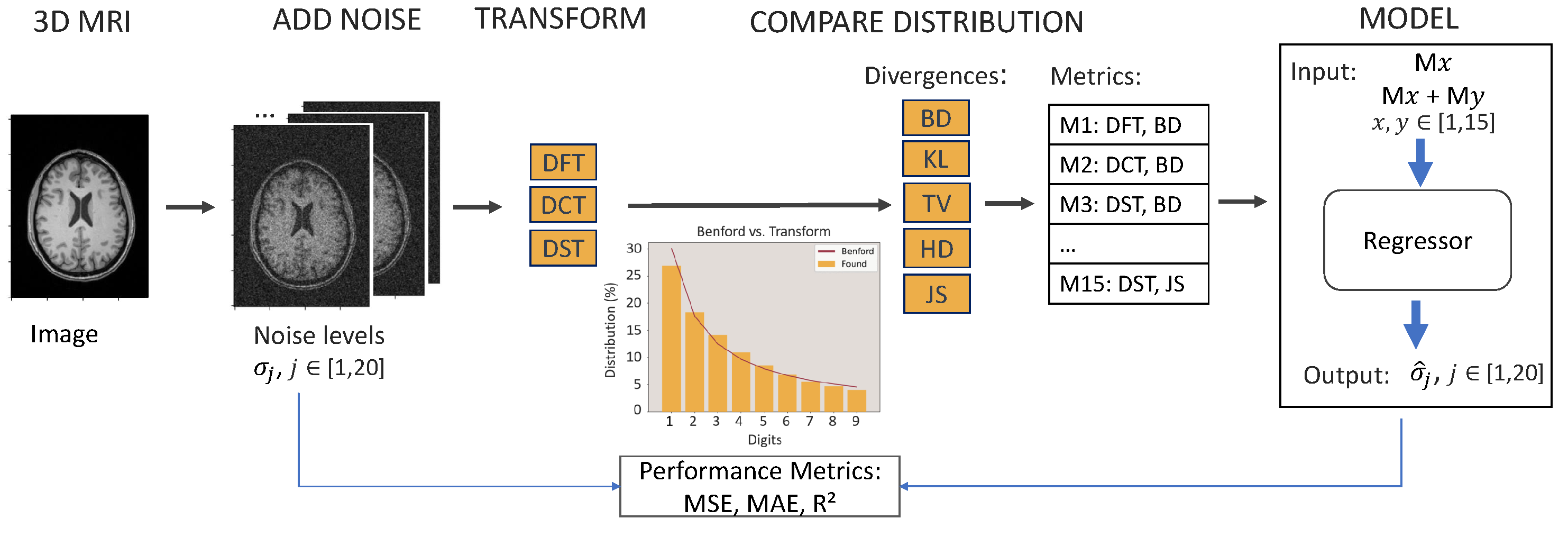
Figure 1.
From left to right, the steps of the algorithm are presented. Images from each repository are noise-added. The noise image is transformed, and the distribution of the first digit appearance is compared with Benford’s Law distribution. The couple transform divergence makes one metric () that will be used as an input on the model. The input can be single or double, and the output is the predicted noise on the image. Three performance metrics are used to measure the success of the model.
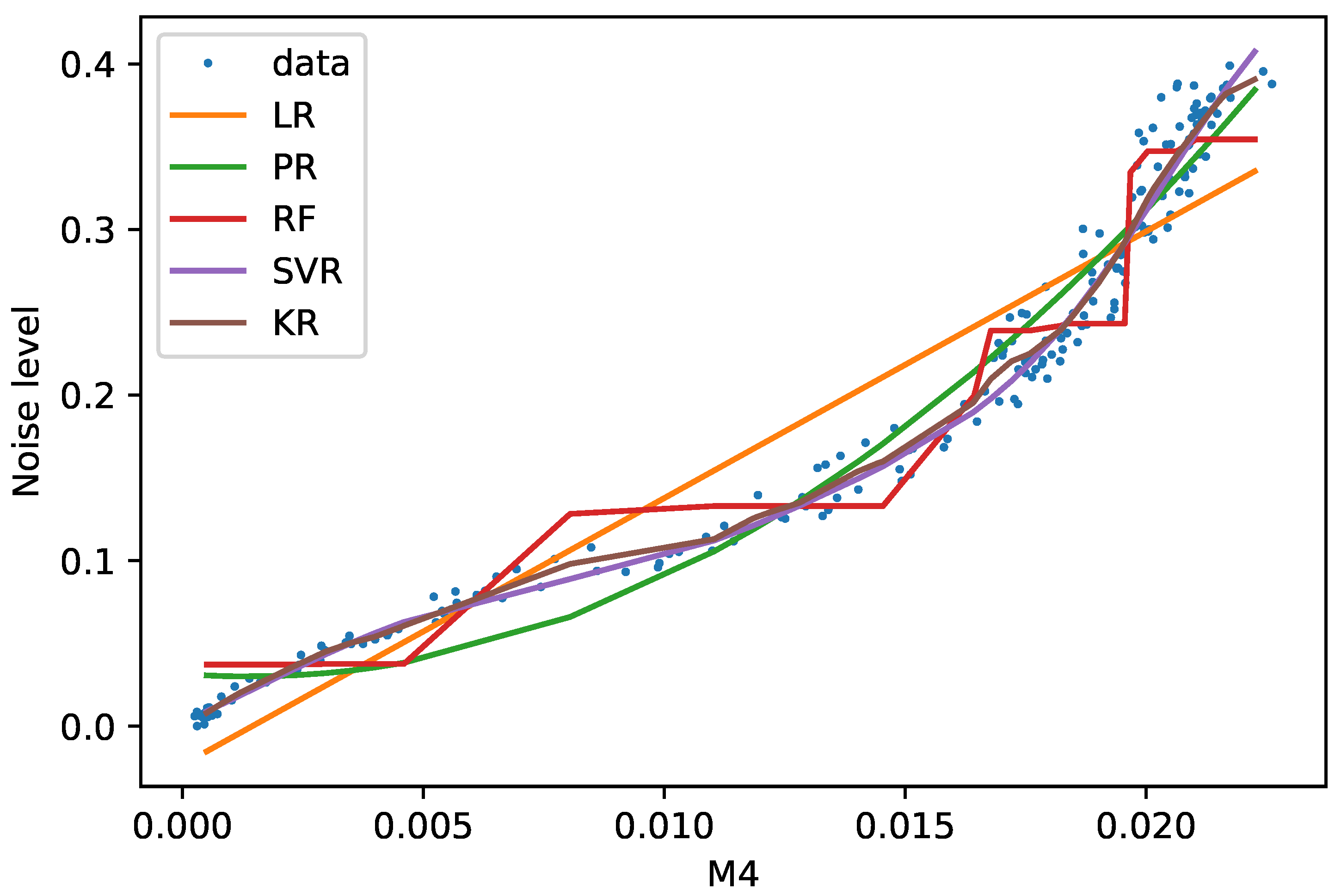
Figure 2.
M4 training data (blue dots) are displayed along with the five models in the HLN repository.
Figure 2.
M4 training data (blue dots) are displayed along with the five models in the HLN repository.
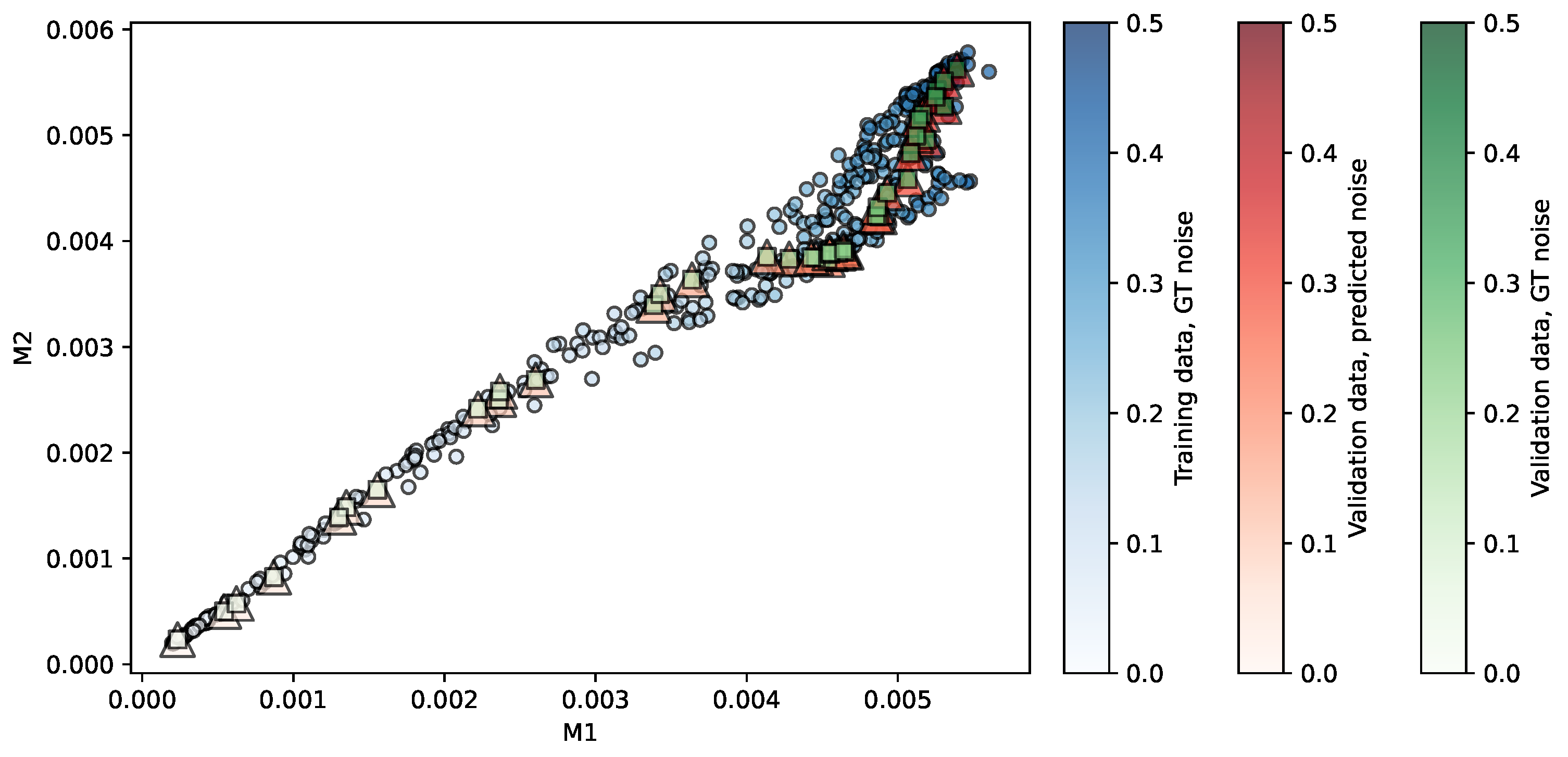
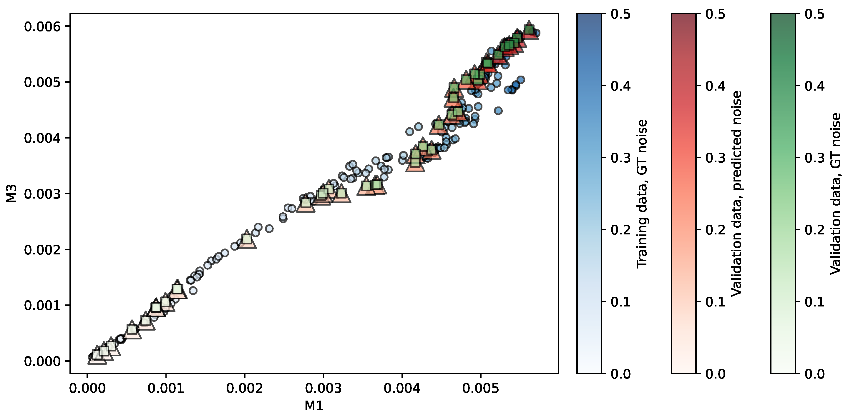
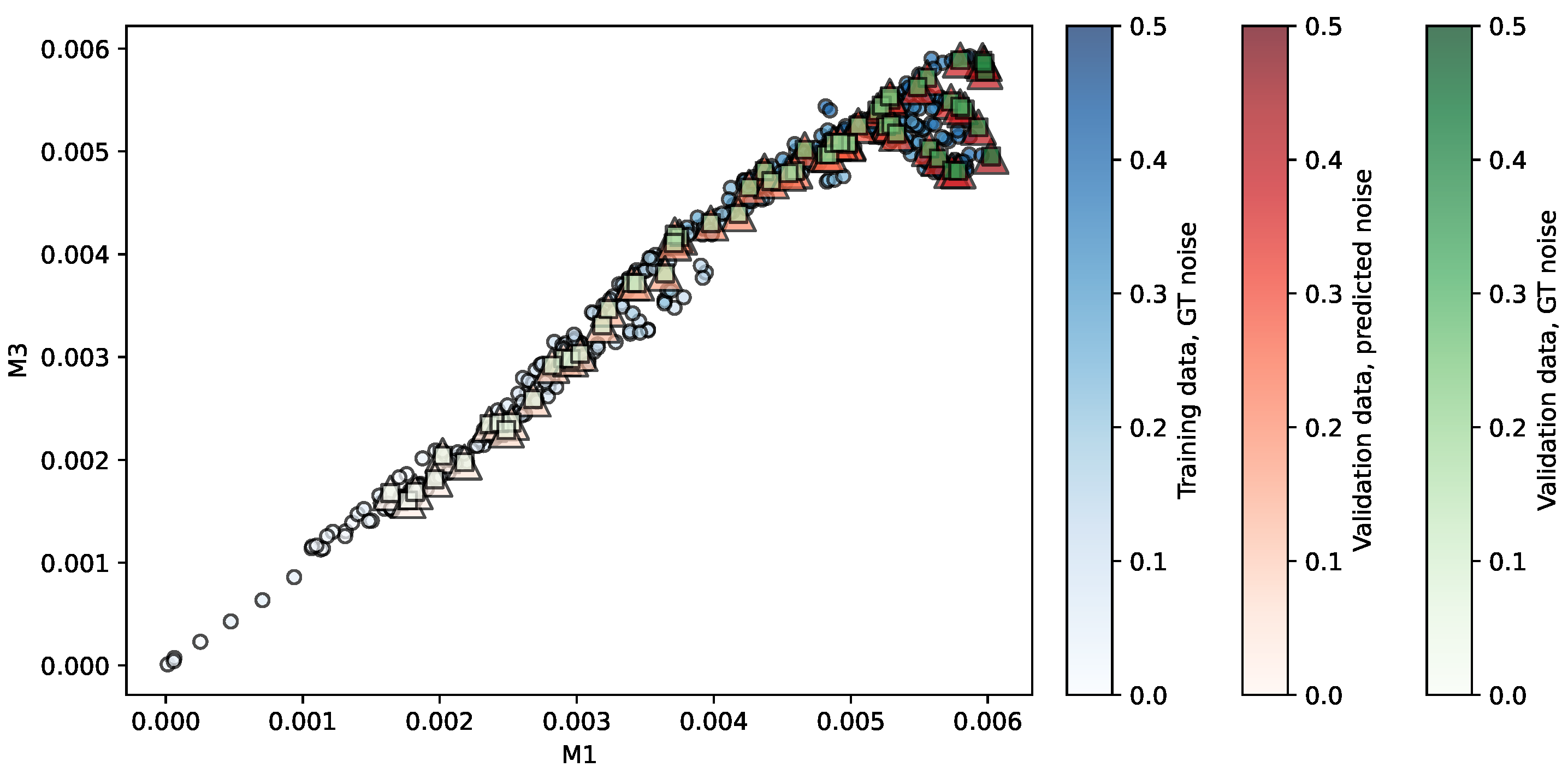
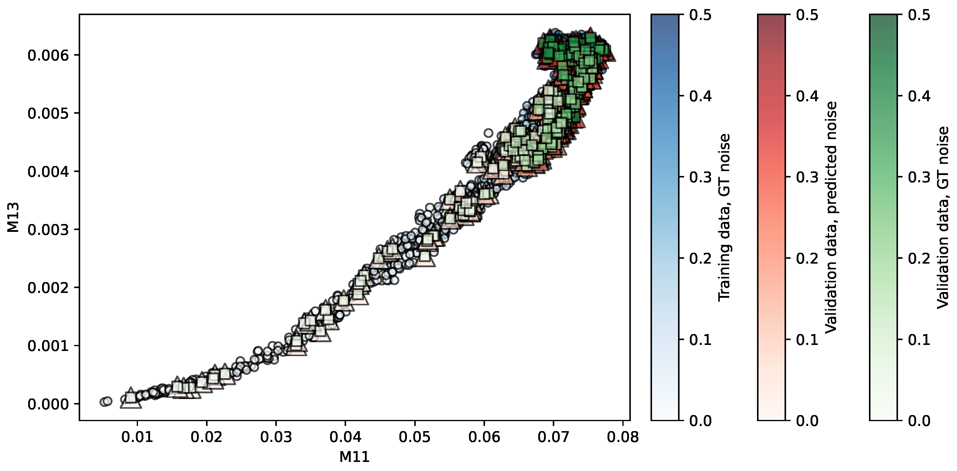
Figure 3.
Regression of the MMRR repository using SVR. Predictors are . The opacity of each shape indicates the noise level associated. More details in the main text.
Figure 3.
Regression of the MMRR repository using SVR. Predictors are . The opacity of each shape indicates the noise level associated. More details in the main text.
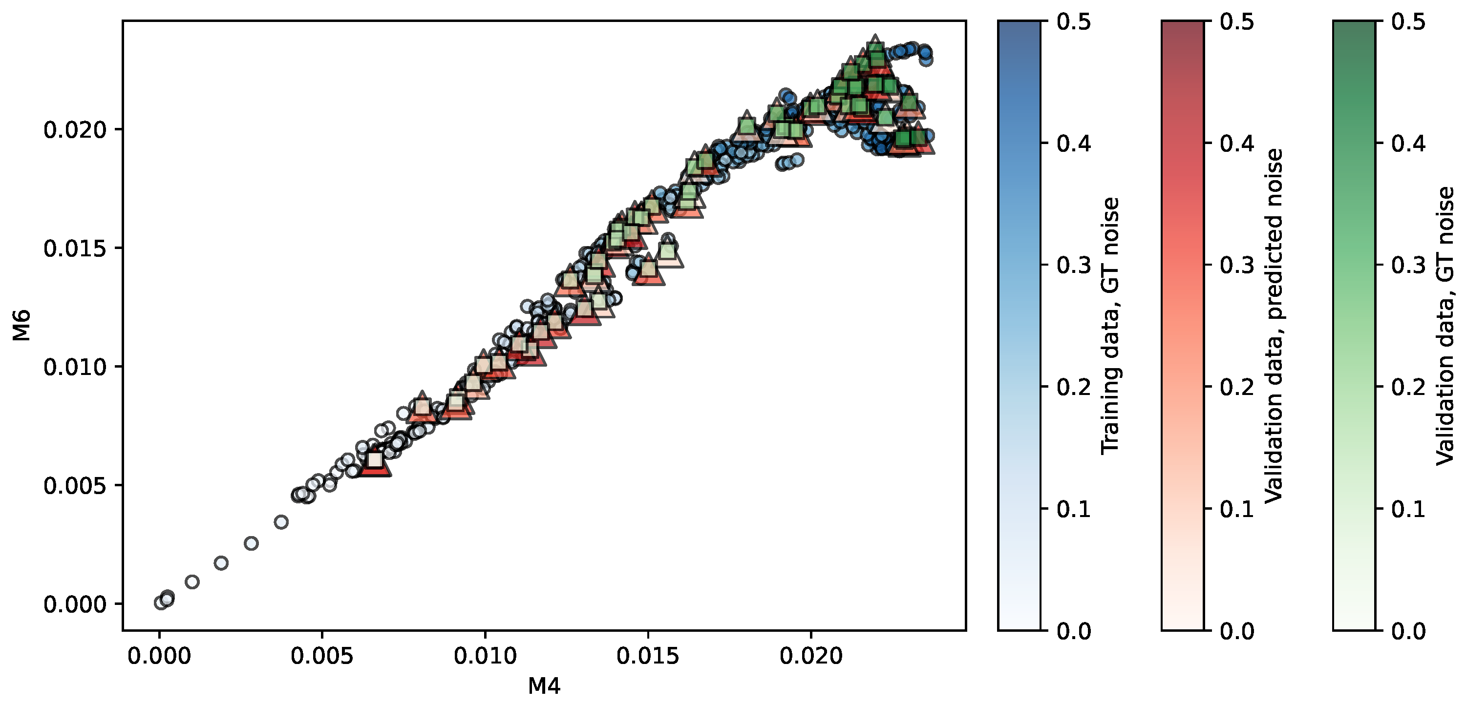
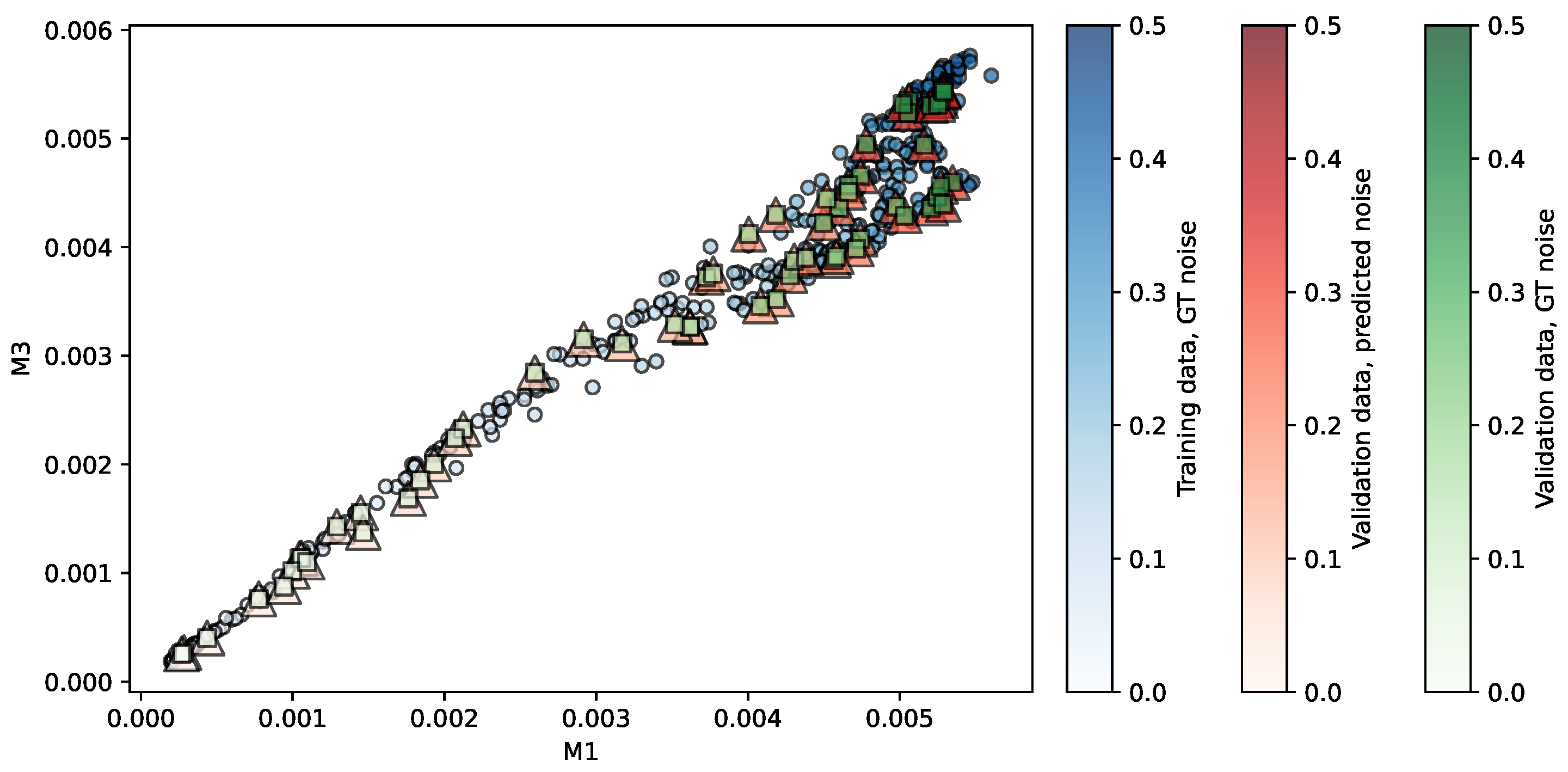
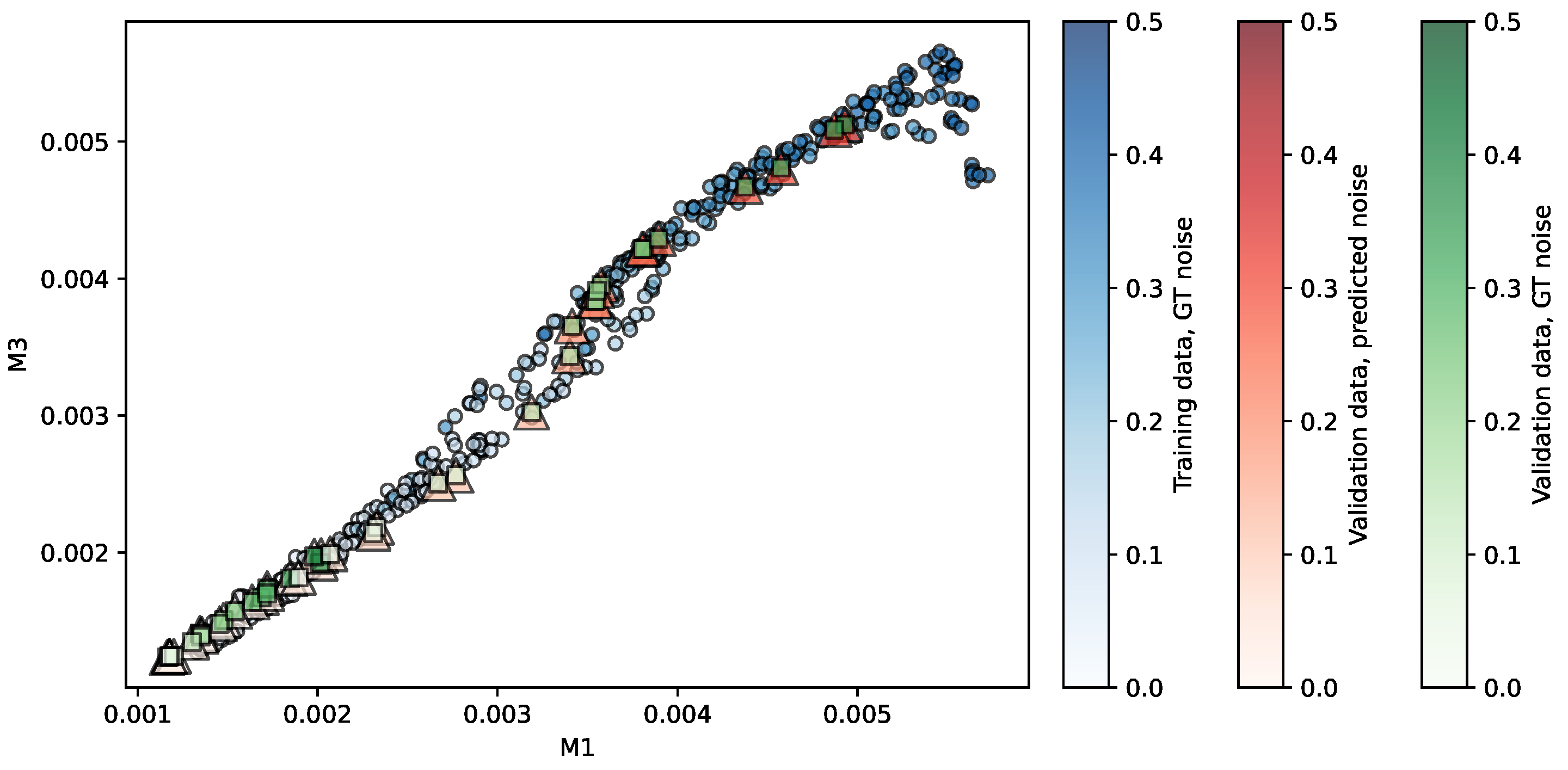
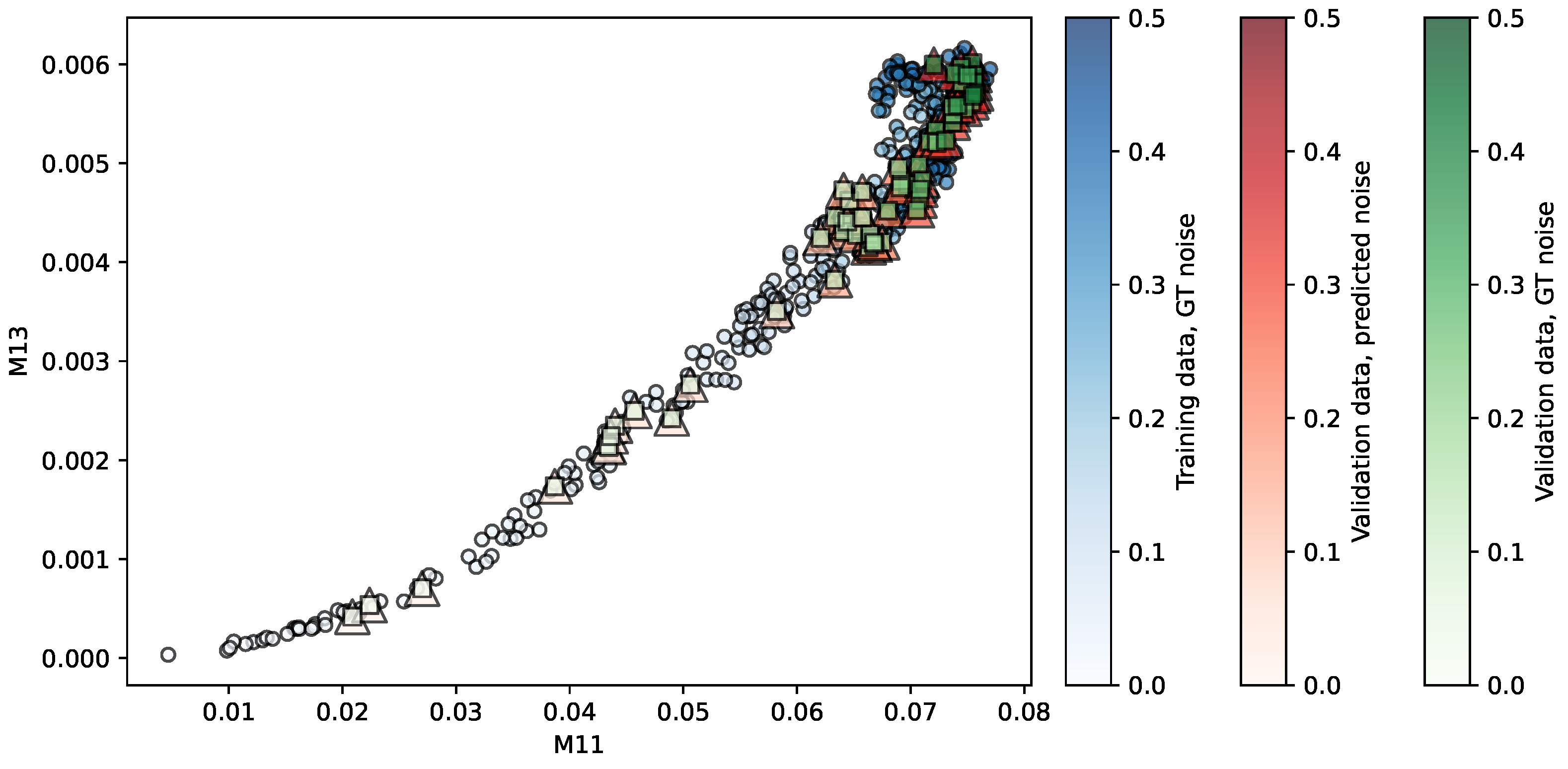
Figure 4.
Regression of the NKI-RS repository using PR. Predictors are . The opacity of each shape indicates the noise level associated.
Figure 4.
Regression of the NKI-RS repository using PR. Predictors are . The opacity of each shape indicates the noise level associated.
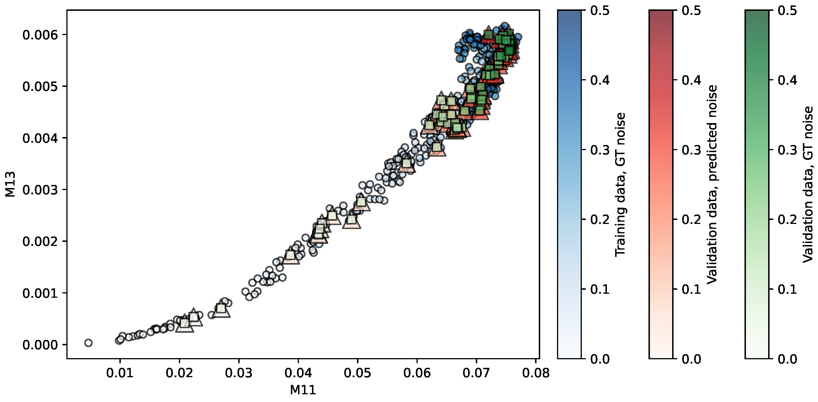
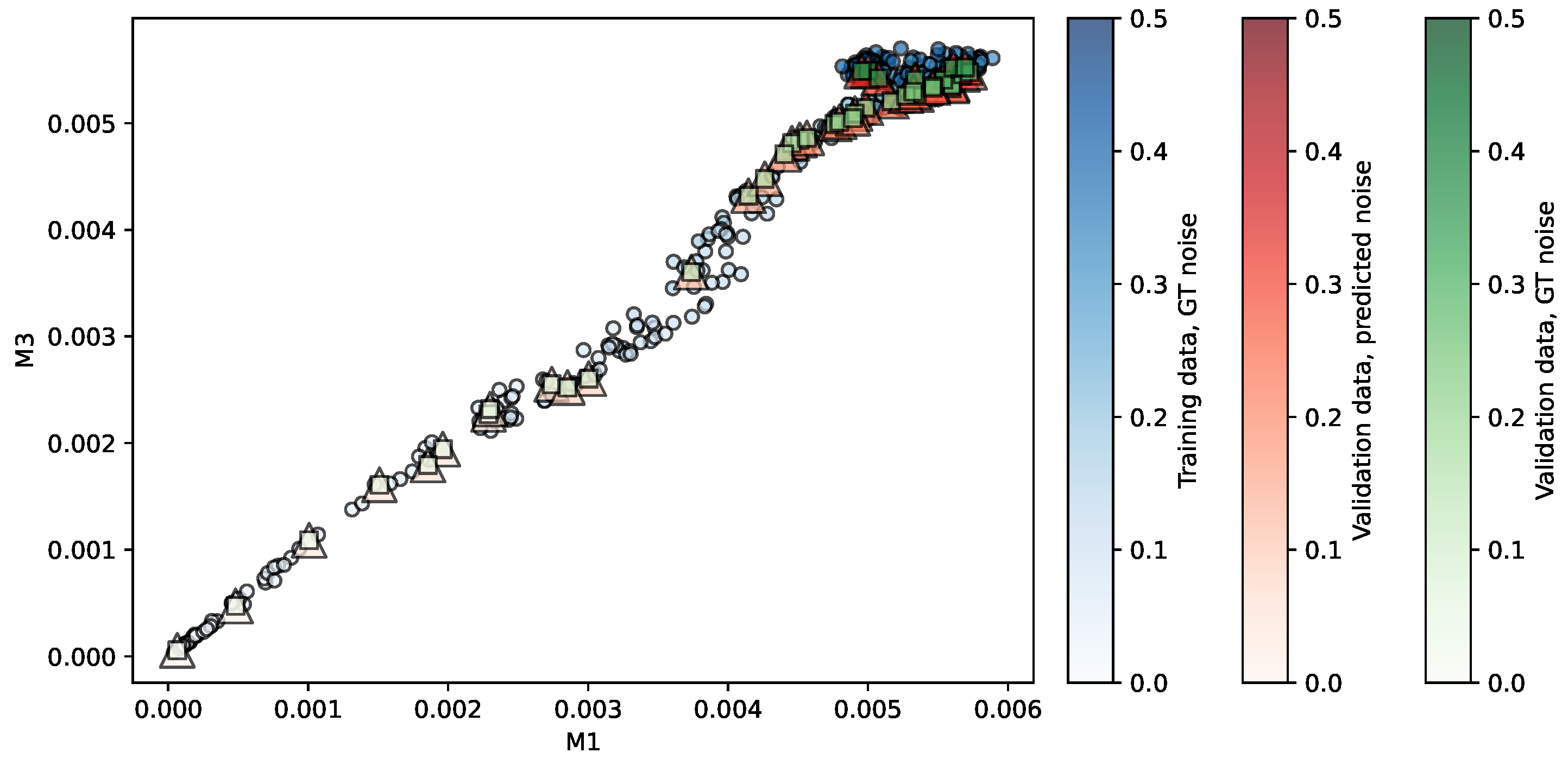
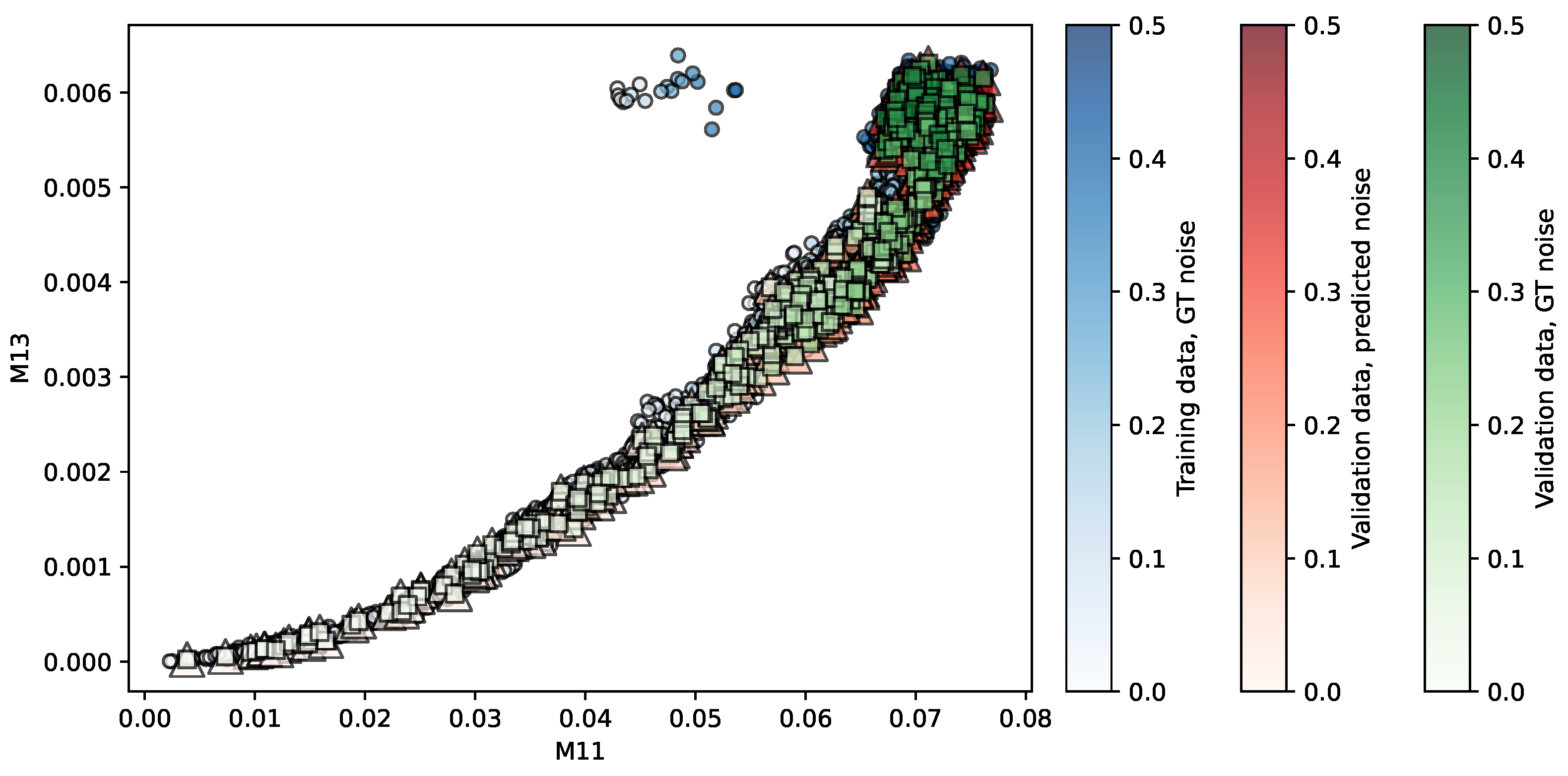
Figure 5.
Regression of the NKI-TRT repository using LR. Predictors are . The opacity of each shape indicates the noise level associated.
Figure 5.
Regression of the NKI-TRT repository using LR. Predictors are . The opacity of each shape indicates the noise level associated.
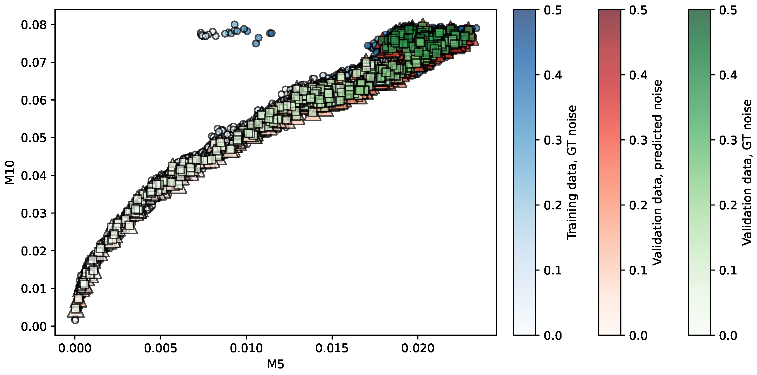
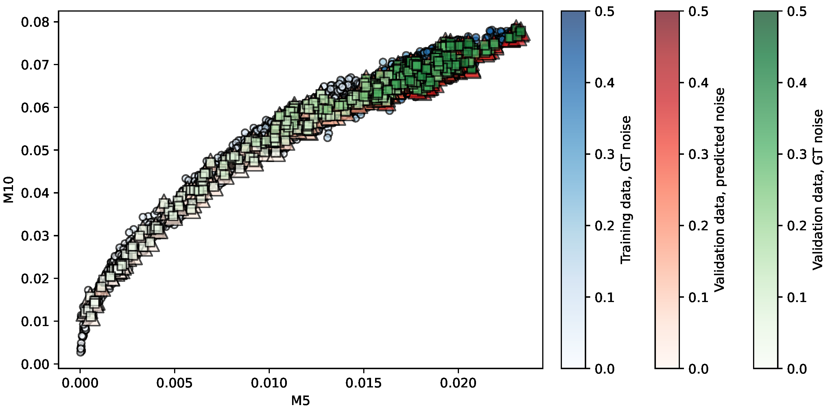
Figure 6.
Regression of the OASIS-TRT repository using KR. Predictors are . The opacity of each shape indicates the noise level associated.
Figure 6.
Regression of the OASIS-TRT repository using KR. Predictors are . The opacity of each shape indicates the noise level associated.
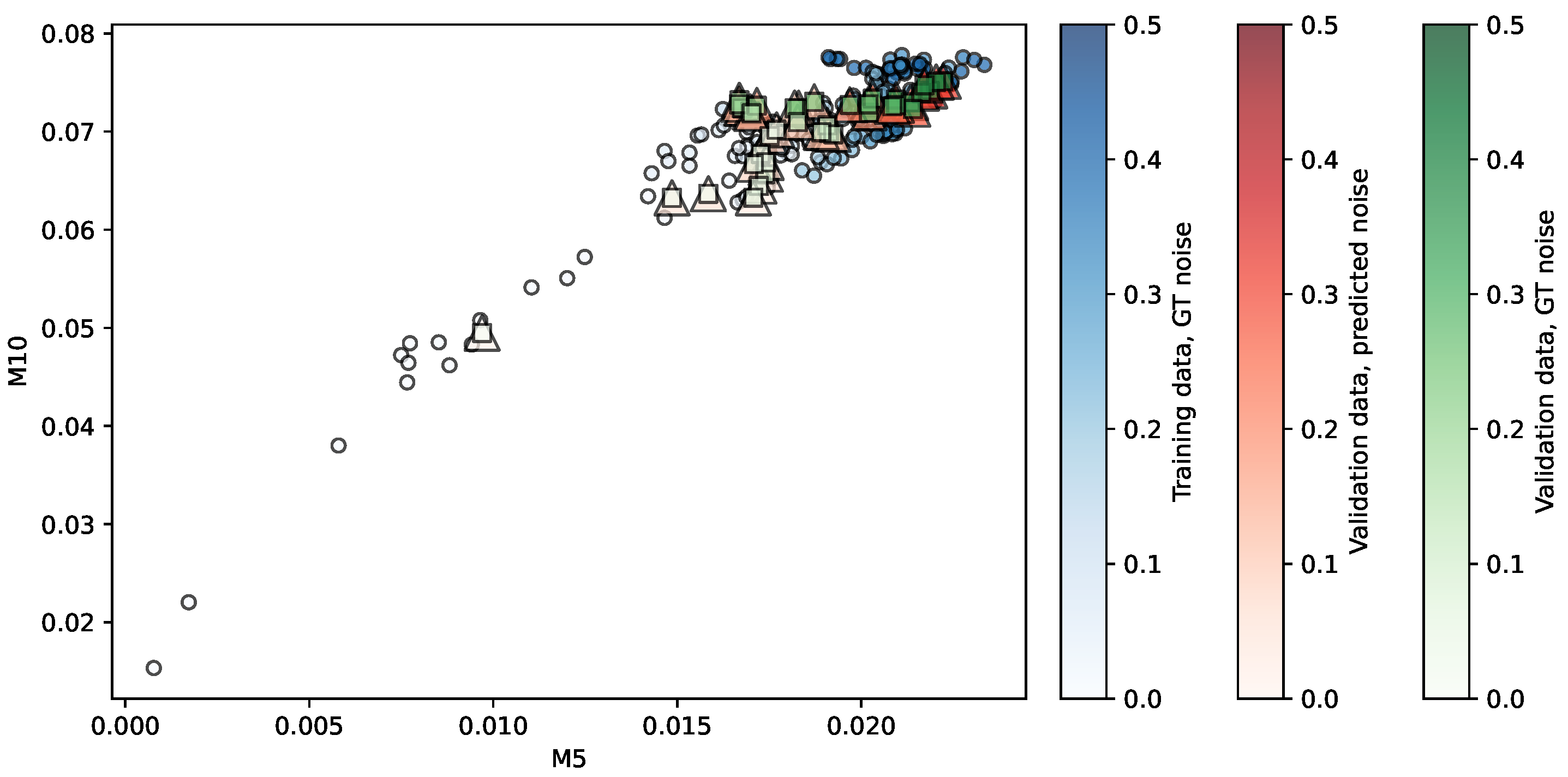
Figure 7.
Regression of the AX-T1 dataset with 1.5 Tesla acquisition using KR. Predictors are . The opacity of each shape indicates the noise level associated.
Figure 7.
Regression of the AX-T1 dataset with 1.5 Tesla acquisition using KR. Predictors are . The opacity of each shape indicates the noise level associated.
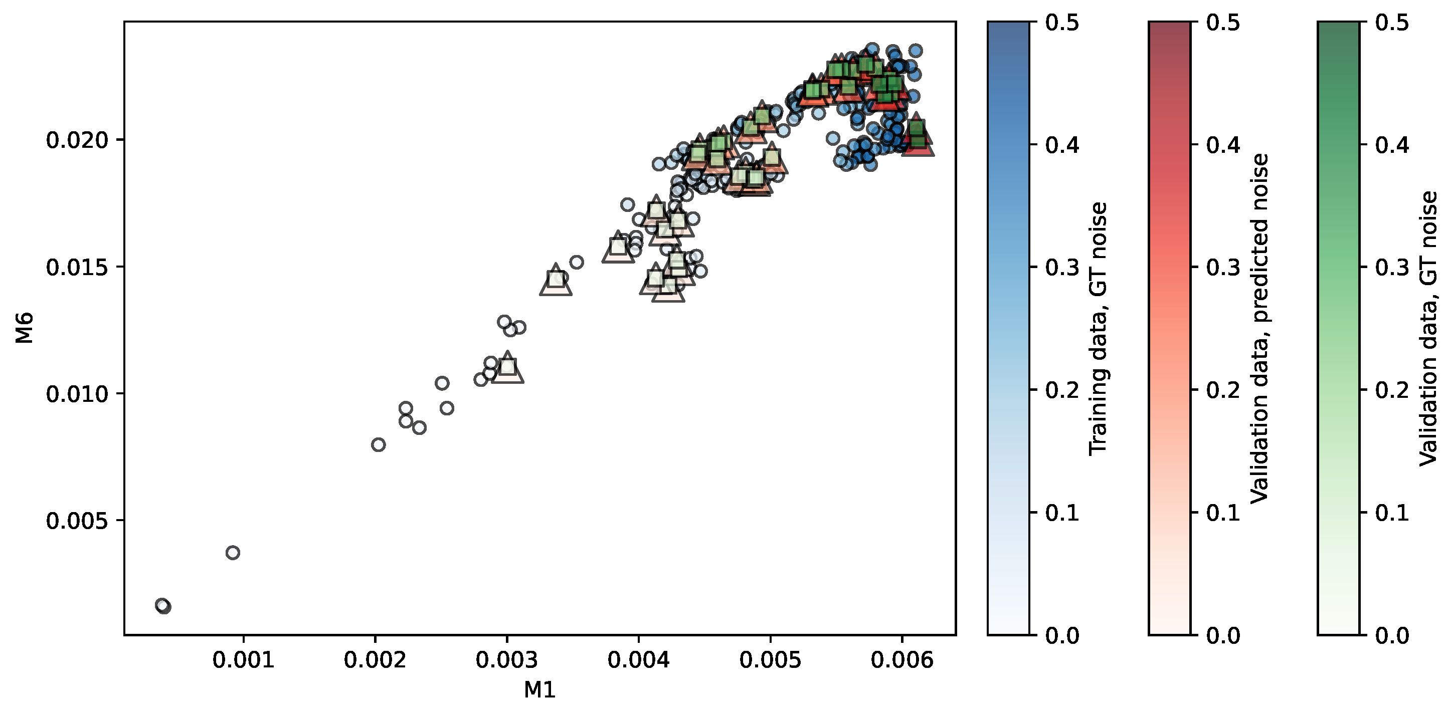
Figure 8.
Regression of the AX-T1-POST dataset with 1.5 Tesla acquisition using SVR. Predictors are . The opacity of each shape indicates the noise level associated.
Figure 8.
Regression of the AX-T1-POST dataset with 1.5 Tesla acquisition using SVR. Predictors are . The opacity of each shape indicates the noise level associated.
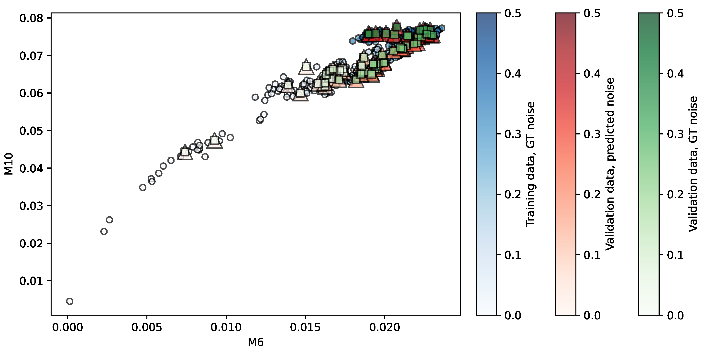
Figure 9.
Regression of the AX-T1-SE dataset with 1.5 Tesla acquisition using SVR. Predictors are . The opacity of each shape indicates the noise level associated.
Figure 9.
Regression of the AX-T1-SE dataset with 1.5 Tesla acquisition using SVR. Predictors are . The opacity of each shape indicates the noise level associated.
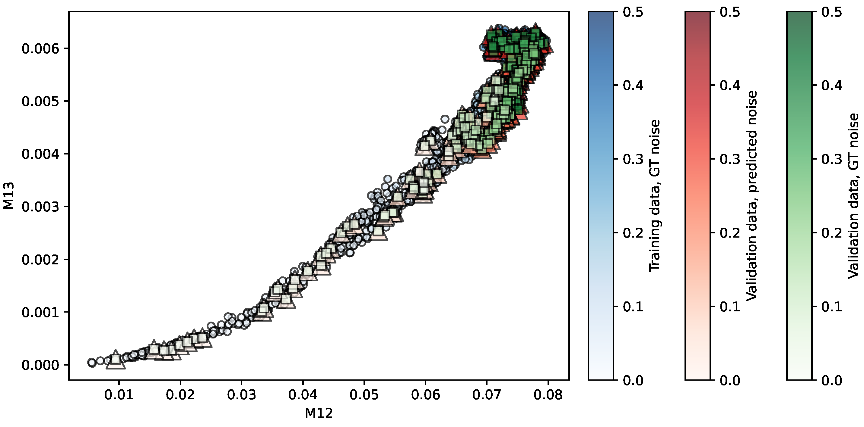
Figure 10.
Regression of the T1-AXIAL dataset with 1.5 Tesla acquisition using KR. Predictors are . The opacity of each shape indicates the noise level associated.
Figure 10.
Regression of the T1-AXIAL dataset with 1.5 Tesla acquisition using KR. Predictors are . The opacity of each shape indicates the noise level associated.
Figure 11.
Regression of the AXIAL-POST-GAD dataset with 1.5 Tesla acquisition using KR. Predictors are . The opacity of each shape indicates the noise level associated.
Figure 11.
Regression of the AXIAL-POST-GAD dataset with 1.5 Tesla acquisition using KR. Predictors are . The opacity of each shape indicates the noise level associated.
Figure 12.
Regression of the AX-T1 dataset using KR (best ranked model). Predictors are . The opacity of each shape indicates the noise level associated.
Figure 12.
Regression of the AX-T1 dataset using KR (best ranked model). Predictors are . The opacity of each shape indicates the noise level associated.
Figure 13.
Regression of the AX-T1-FLASH-POST dataset using KR (best ranked model). Predictors are . The opacity of each shape indicates the noise level associated.
Figure 13.
Regression of the AX-T1-FLASH-POST dataset using KR (best ranked model). Predictors are . The opacity of each shape indicates the noise level associated.
Figure 14.
Regression of the AX-T1-POST dataset using KR (best ranked model). Predictors are . The opacity of each shape indicates the noise level associated.
Figure 14.
Regression of the AX-T1-POST dataset using KR (best ranked model). Predictors are . The opacity of each shape indicates the noise level associated.
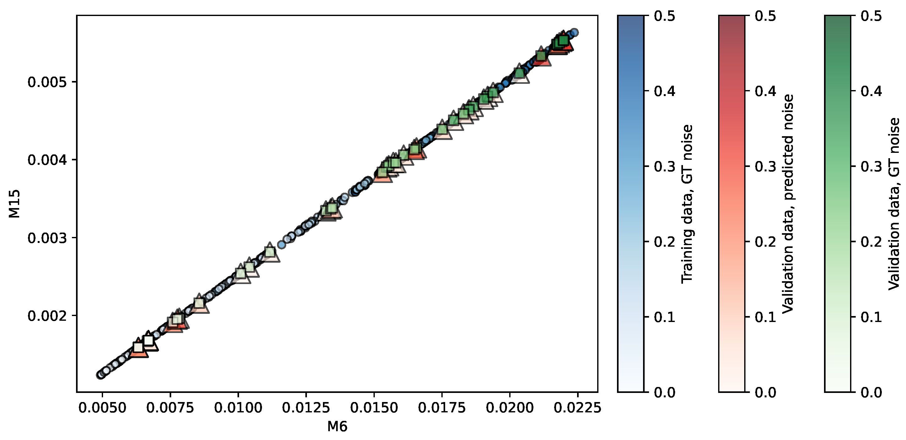
Figure 15.
Regression of the HLN repository using SVR (best ranked model). Predictors are . The opacity of each shape indicates the noise level associated.
Figure 15.
Regression of the HLN repository using SVR (best ranked model). Predictors are . The opacity of each shape indicates the noise level associated.
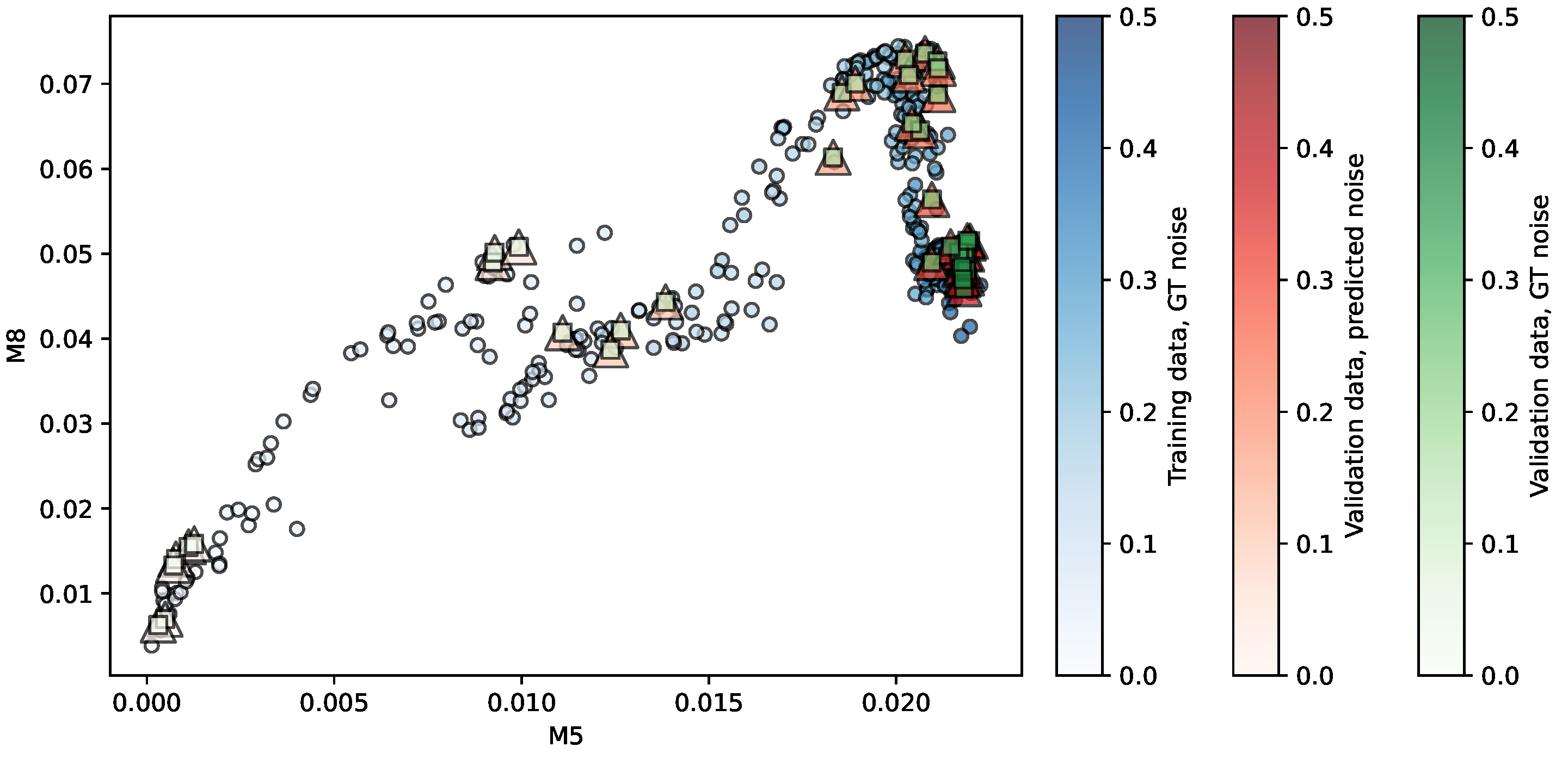
Figure 16.
Regression of the MMRR repository using SVR (best ranked model). Predictors are . The opacity of each shape indicates the noise level associated.
Figure 16.
Regression of the MMRR repository using SVR (best ranked model). Predictors are . The opacity of each shape indicates the noise level associated.
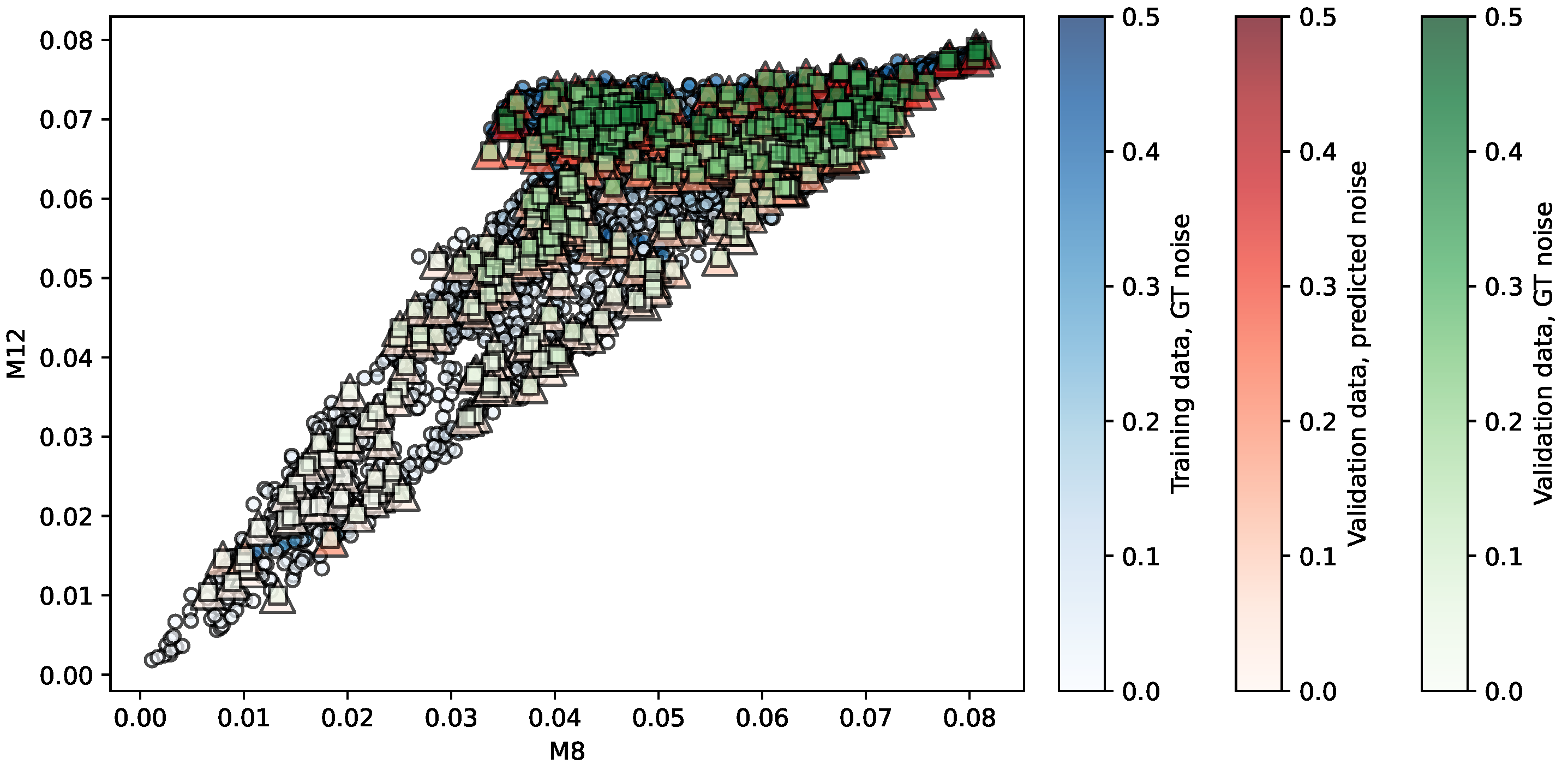
Figure 17.
Regression of the NKI-RS repository using SVR (best ranked model). Predictors are . The opacity of each shape indicates the noise level associated.
Figure 17.
Regression of the NKI-RS repository using SVR (best ranked model). Predictors are . The opacity of each shape indicates the noise level associated.
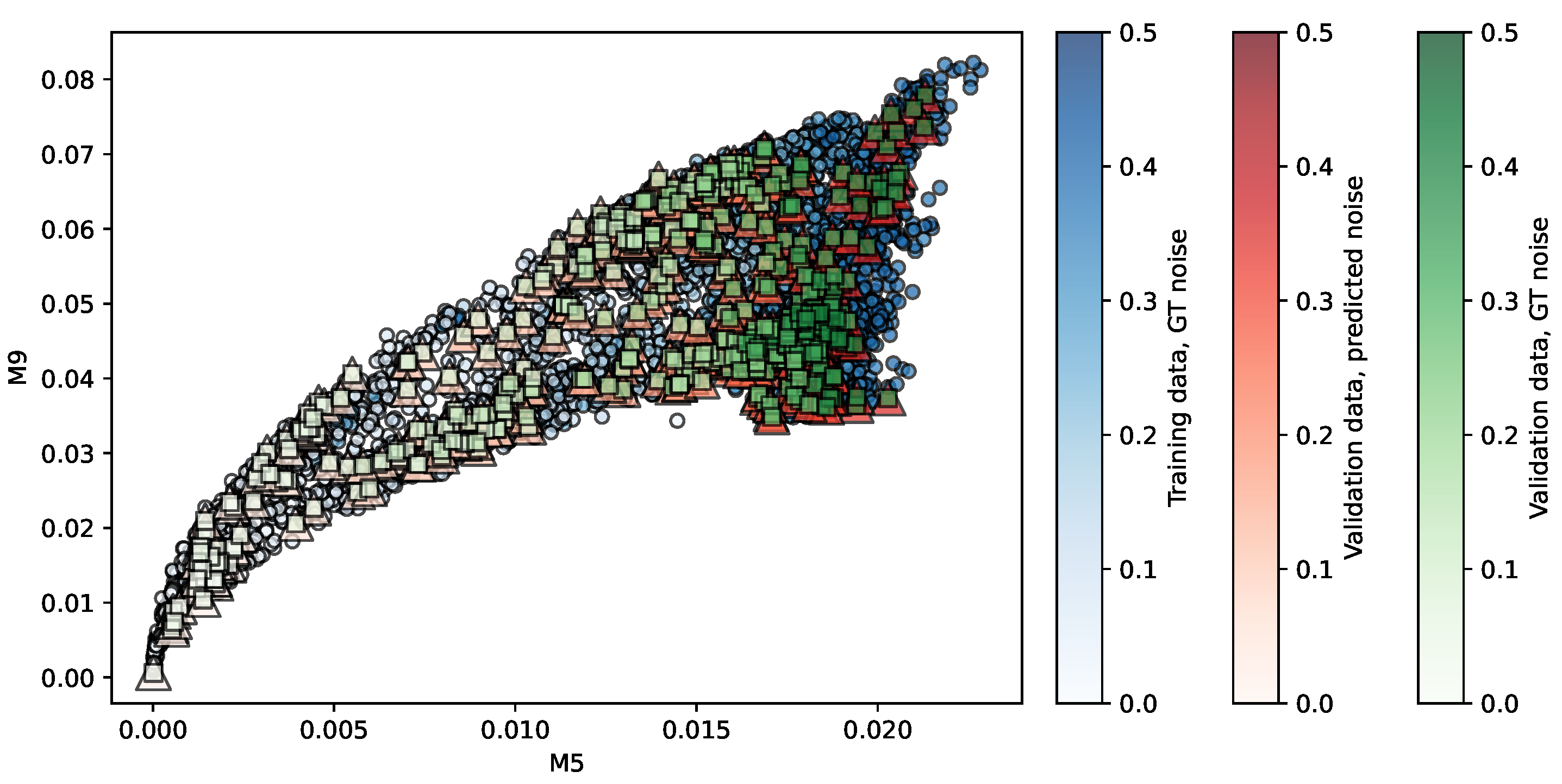
Figure 18.
Regression of the NKI-TRT repository using SVR (best ranked model). Predictors are . The opacity of each shape indicates the noise level associated.
Figure 18.
Regression of the NKI-TRT repository using SVR (best ranked model). Predictors are . The opacity of each shape indicates the noise level associated.
Figure 19.
Regression of the OASIS-TRT repository using SVR (best ranked model). Predictors are . The opacity of each shape indicates the noise level associated.
Figure 19.
Regression of the OASIS-TRT repository using SVR (best ranked model). Predictors are . The opacity of each shape indicates the noise level associated.
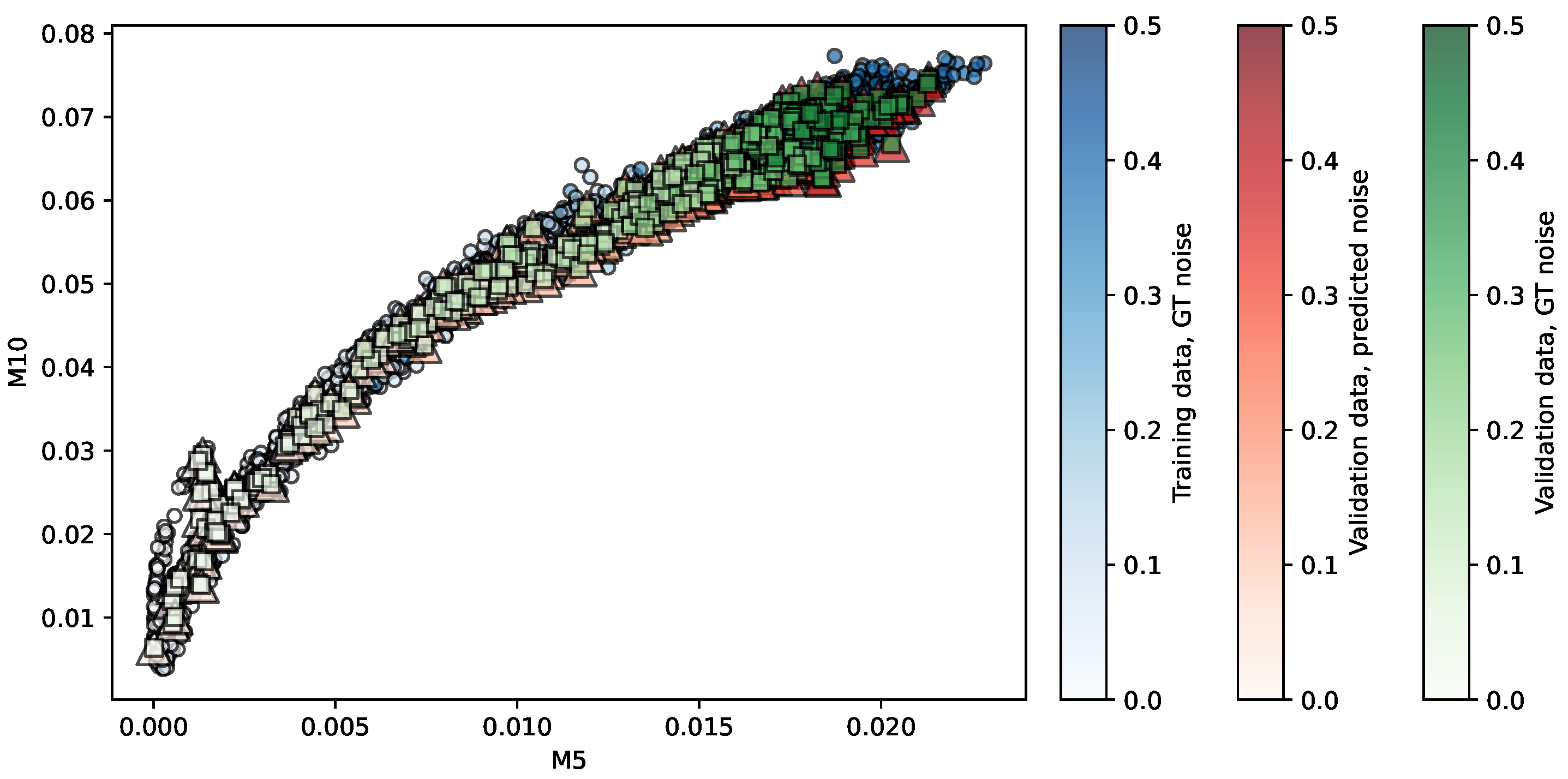
Figure 20.
Regression of the AX-T1-1.5 dataset using SVR (best ranked model). Predictors are . The opacity of each shape indicates the noise level associated.
Figure 20.
Regression of the AX-T1-1.5 dataset using SVR (best ranked model). Predictors are . The opacity of each shape indicates the noise level associated.
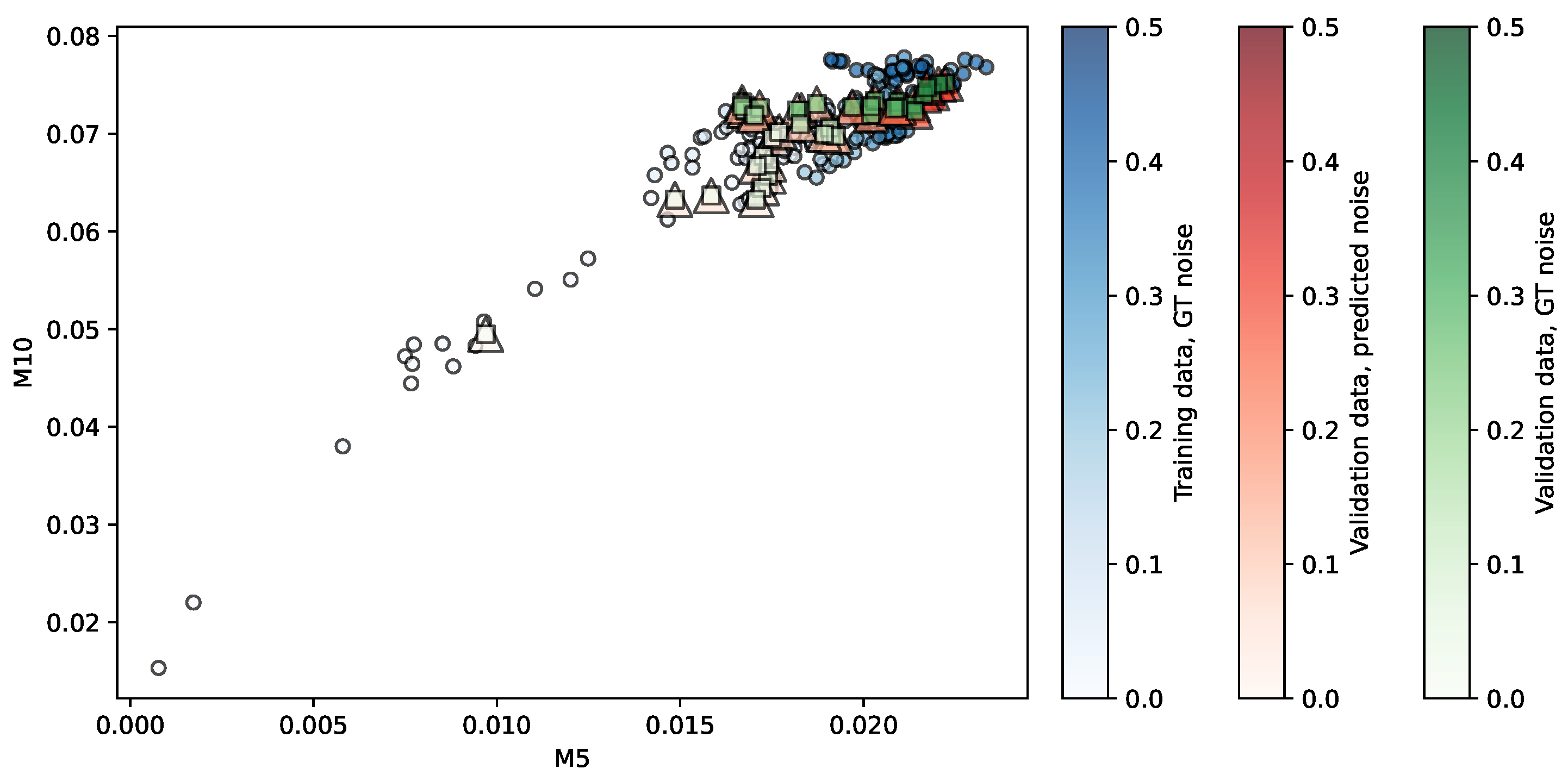
Figure 21.
Regression of the AX-T1-POST-1.5 dataset using SVR (best ranked model). Predictors are . The opacity of each shape indicates the noise level associated.
Figure 21.
Regression of the AX-T1-POST-1.5 dataset using SVR (best ranked model). Predictors are . The opacity of each shape indicates the noise level associated.
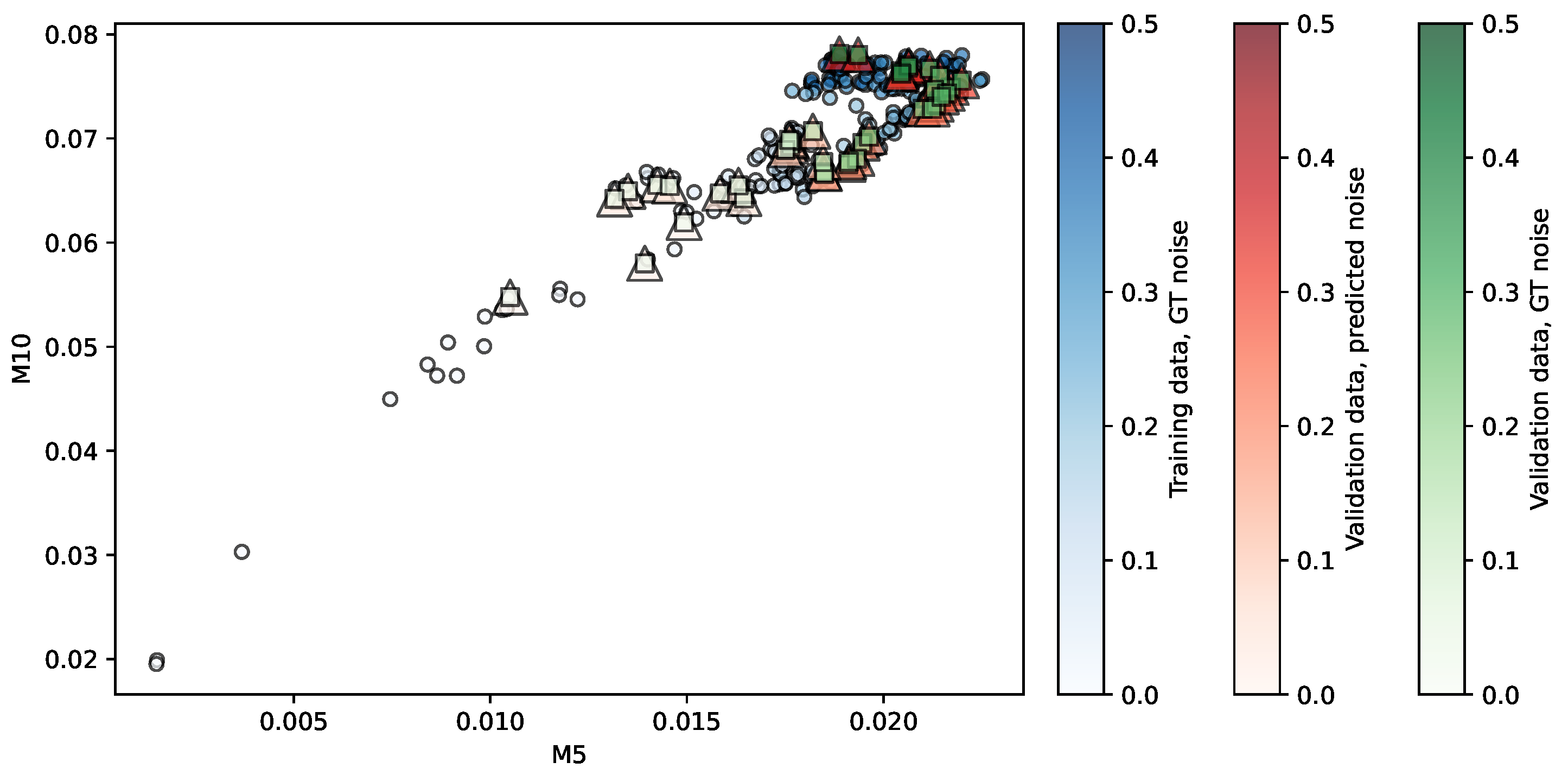
Figure 22.
Regression of the AX-T1-SE dataset using SVR (best ranked model). Predictors are . The opacity of each shape indicates the noise level associated.
Figure 22.
Regression of the AX-T1-SE dataset using SVR (best ranked model). Predictors are . The opacity of each shape indicates the noise level associated.
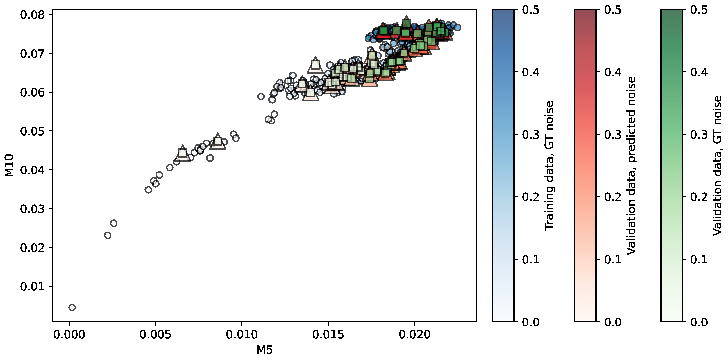
Figure 23.
Regression of the T1-AXIAL dataset using SVR (best ranked model). Predictors are . The opacity of each shape indicates the noise level associated.
Figure 23.
Regression of the T1-AXIAL dataset using SVR (best ranked model). Predictors are . The opacity of each shape indicates the noise level associated.
Figure 24.
Regression of the T1-AXIAL-POST-GAD dataset using SVR (best ranked model). Predictors are . The opacity of each shape indicates the noise level associated.
Figure 24.
Regression of the T1-AXIAL-POST-GAD dataset using SVR (best ranked model). Predictors are . The opacity of each shape indicates the noise level associated.
Figure 25.
Regression of the AX-T1 dataset with 3 Tesla acquisitions using SVR (best ranked model). Predictors are . The opacity of each shape indicates the noise level associated.
Figure 25.
Regression of the AX-T1 dataset with 3 Tesla acquisitions using SVR (best ranked model). Predictors are . The opacity of each shape indicates the noise level associated.
Figure 26.
Regression of the AX-T1-FLASH-POST dataset with 3 Tesla acquisitions using SVR (best ranked model). Predictors are . The opacity of each shape indicates the noise level associated.
Figure 26.
Regression of the AX-T1-FLASH-POST dataset with 3 Tesla acquisitions using SVR (best ranked model). Predictors are . The opacity of each shape indicates the noise level associated.
Figure 27.
Regression of the AX-T1-POST dataset with 3 Tesla acquisitions using SVR (best ranked model). Predictors are . The opacity of each shape indicates the noise level associated.
Figure 27.
Regression of the AX-T1-POST dataset with 3 Tesla acquisitions using SVR (best ranked model). Predictors are . The opacity of each shape indicates the noise level associated.
Table 1.
Noise levels () used in this work and the induced SNR of the noisy images in the 12HLN repository.
Table 1.
Noise levels () used in this work and the induced SNR of the noisy images in the 12HLN repository.
| Average SNR | | Average SNR |
|---|
| 0.02 | 521.80 | 0.22 | 5.30 |
| 0.04 | 131.19 | 0.24 | 4.62 |
| 0.06 | 58.86 | 0.26 | 4.08 |
| 0.08 | 33.55 | 0.28 | 3.66 |
| 0.10 | 21.83 | 0.30 | 3.31 |
| 0.12 | 15.47 | 0.32 | 3.03 |
| 0.14 | 11.63 | 0.34 | 2.80 |
| 0.16 | 9.14 | 0.36 | 2.61 |
| 0.18 | 7.43 | 0.38 | 2.44 |
| 0.20 | 6.21 | 0.40 | 2.30 |
Table 2.
Definitions of metric variables, specifying the transformation and dissimilarity measures used.
Table 2.
Definitions of metric variables, specifying the transformation and dissimilarity measures used.
| Metrics | Transformation | Dissimilarity |
|---|
| M1 | DFT | BD |
| M2 | DCT | BD |
| M3 | DST | BD |
| M4 | DFT | KL |
| M5 | DCT | KL |
| M6 | DST | KL |
| M7 | DFT | TV |
| M8 | DCT | TV |
| M9 | DST | TV |
| M10 | DFT | HD |
| M11 | DCT | HD |
| M12 | DST | HD |
| M13 | DFT | JS |
| M14 | DCT | JS |
| M15 | DST | JS |
Table 3.
Goodness-of-fit of noise level regression in the Mindboggle dataset. The metrics are globally ranked by the value. For the sake of readability, is scaled up by a factor of in this table. Best-performing regressors are in brackets.
Table 3.
Goodness-of-fit of noise level regression in the Mindboggle dataset. The metrics are globally ranked by the value. For the sake of readability, is scaled up by a factor of in this table. Best-performing regressors are in brackets.
| Metrics | Score | HLN | MMRR | NKI-RS | NKI-TRT | OASIS-TRT |
|---|
| M1 + M3 | 473 | 3.04 (KR) | 2.51 (SVR) | 11.36 (PR) | 37.16 (PR) | 7.18 (RF) |
| M3 + M13 | 468 | 3.04 (KR) | 2.50 (SVR) | 11.35 (PR) | 37.17 (PR) | 7.28 (RF) |
| M1 + M15 | 468 | 3.04 (KR) | 2.50 (SVR) | 11.36 (PR) | 37.17 (PR) | 7.23 (RF) |
| M13 + M15 | 462 | 3.04 (KR) | 2.51 (SVR) | 11.35 (PR) | 37.17 (PR) | 7.23 (RF) |
| M3 + M4 | 456 | 3.21 (KR) | 2.55 (SVR) | 11.25 (PR) | 37.21 (PR) | 7.21 (KR) |
| M4 + M15 | 453 | 3.23 (KR) | 2.54 (SVR) | 11.13 (PR) | 37.21 (PR) | 7.22 (RF) |
| M2 + M4 | 445 | 3.25 (KR) | 2.56 (SVR) | 11.33 (PR) | 37.58 (PR) | 6.79 (KR) |
| M4 + M14 | 444 | 3.26 (KR) | 2.55 (SVR) | 11.34 (PR) | 37.58 (PR) | 6.84 (KR) |
| M1 + M2 | 433 | 3.02 (KR) | 2.49 (SVR) | 11.46 (PR) | 37.53 (PR) | 7.69 (SVR) |
| M13 + M14 | 432 | 3.02 (KR) | 2.49 (SVR) | 11.45 (PR) | 37.54 (PR) | 7.67 (SVR) |
Table 4.
Goodness-of-fit of noise level regression in the Mindboggle dataset. The metrics are globally ranked by the value, scaled up by a factor of in this table.
Table 4.
Goodness-of-fit of noise level regression in the Mindboggle dataset. The metrics are globally ranked by the value, scaled up by a factor of in this table.
| Metrics | Score | HLN | MMRR | NKI-RS | NKI-TRT | OASIS-TRT |
|---|
| M12 + M13 | 499 | 12.57 (PR) | 10.95 (SVR) | 26.36 (RF) | 36.77 (SVR) | 19.50 (KR) |
| M1 + M12 | 496 | 12.58 (PR) | 10.92 (SVR) | 26.39 (RF) | 36.78 (SVR) | 19.51 (KR) |
| M3 + M4 | 492 | 12.93 (SVR) | 11.06 (SVR) | 26.23 (RF) | 36.82 (SVR) | 18.97 (KR) |
| M4 + M15 | 488 | 12.92 (SVR) | 11.04 (SVR) | 26.33 (RF) | 36.89 (SVR) | 19.03 (KR) |
| M1 +M11 | 480 | 12.57 (PR) | 10.97 (SVR) | 26.71 (RF) | 37.35 (SVR) | 18.81 (KR) |
| M11 + M13 | 474 | 12.58 (PR) | 10.99 (SVR) | 26.75 (RF) | 37.34 (SVR) | 18.81 (KR) |
| M1 + M3 | 473 | 13.27 (SVR) | 10.96 (SVR) | 26.32 (RF) | 36.68 (SVR) | 19.80 (RF) |
| M3 + M13 | 470 | 13.21 (SVR) | 10.95 (SVR) | 26.19 (RF) | 36.71 (SVR) | 19.88 (RF) |
| M6 + M13 | 469 | 13.15 (KR) | 11.05 (SVR) | 26.50 (RF) | 36.60 (SVR) | 19.50 (KR) |
| M1 + M15 | 468 | 13.21 (KR) | 10.95 (SVR) | 26.34 (RF) | 36.68 (SVR) | 19.85 (RF) |
Table 5.
of the regression models on the Mindboggle dataset.
Table 5.
of the regression models on the Mindboggle dataset.
| Metrics | Score | HLN | MMRR | NKI-RS | NKI-TRT | OASIS-TRT |
|---|
| M1 + M3 | 477 | 0.9785 (KR) | 0.9821 (SVR) | 0.9125 (PR) | 0.6952 (PR) | 0.9444 (RF) |
| M1 + M15 | 472 | 0.9785 (KR) | 0.9822 (SVR) | 0.9125 (PR) | 0.6952 (PR) | 0.9441 (RF) |
| M3 + M13 | 469 | 0.9785 (KR) | 0.9822 (SVR) | 0.9125 (PR) | 0.6951 (PR) | 0.9437 (RF) |
| M13 + M15 | 462 | 0.9785 (KR) | 0.9821 (SVR) | 0.9125 (PR) | 0.6951 (PR) | 0.9440 (RF) |
| M4 + M15 | 458 | 0.9774 (SVR) | 0.9819 (SVR) | 0.9133 (PR) | 0.6944 (PR) | 0.9443 (RF) |
| M3 + M4 | 456 | 0.9775 (KR) | 0.9818 (SVR) | 0.9133 (PR) | 0.6944 (PR) | 0.9443 (RF) |
| M4 + M14 | 442 | 0.9772 (KR) | 0.9818 (SVR) | 0.9127 (PR) | 0.6914 (PR) | 0.9463 (KR) |
| M2 + M4 | 442 | 0.9772 (KR) | 0.9817 (SVR) | 0.9127 (PR) | 0.6914 (PR) | 0.9466 (KR) |
| M1 + M11 | 436 | 0.9803 (PR) | 0.9821 (SVR) | 0.9085 (RF) | 0.6880 (PR) | 0.9462 (KR) |
| M11 + M13 | 436 | 0.9803 (PR) | 0.9821 (SVR) | 0.9084 (RF) | 0.6880 (PR) | 0.9462 (KR) |
Table 6.
Goodness-of-fit of noise level regression in the fastMRI dataset with 1.5 Tesla acquisition. The metrics are globally ranked by the value, scaled up by a factor of in this table.
Table 6.
Goodness-of-fit of noise level regression in the fastMRI dataset with 1.5 Tesla acquisition. The metrics are globally ranked by the value, scaled up by a factor of in this table.
| Metrics | Score | T1_AXIAL_POST_GAD | Axial_T1_SE | T1_AXIAL | AX_T1_POST_15 | AX_T1_15 |
|---|
| M5 + M10 | 530 | 7.83 (KR) | 20.71 (SVR) | 9.56 (SVR) | 17.92 (SVR) | 35.95 (KR) |
| M2 + M10 | 527 | 8.06 (KR) | 20.94 (SVR) | 9.54 (SVR) | 17.92 (SVR) | 35.88 (KR) |
| M10 + M14 | 525 | 8.05 (KR) | 20.96 (SVR) | 9.53 (SVR) | 17.92 (SVR) | 35.89 (KR) |
| M1 + M5 | 518 | 8.21 (SVR) | 21.57 (SVR) | 9.45 (KR) | 17.91 (SVR) | 36.33 (RF) |
| M5 + M13 | 511 | 8.20 (SVR) | 21.53 (SVR) | 9.46 (KR) | 17.92 (SVR) | 36.36 (RF) |
| M4 + M5 | 486 | 8.43 (SVR) | 21.99 (SVR) | 9.63 (SVR) | 17.90 (SVR) | 36.57 (RF) |
| M2 + M13 | 484 | 8.51 (SVR) | 23.04 (SVR) | 9.59 (SVR) | 17.93 (SVR) | 36.22 (RF) |
| M13 + M14 | 479 | 8.53 (SVR) | 22.90 (SVR) | 9.64 (SVR) | 17.93 (SVR) | 36.15 (RF) |
| M6 + M13 | 478 | 7.88 (SVR) | 23.14 (SVR) | 9.14 (KR) | 18.45 (SVR) | 35.90 (RF) |
Table 7.
Goodness-of-fit of noise level regression in the fastMRI dataset with 1.5 Tesla acquisition. The metrics are globally ranked by the value, scaled up by a factor of in this table.
Table 7.
Goodness-of-fit of noise level regression in the fastMRI dataset with 1.5 Tesla acquisition. The metrics are globally ranked by the value, scaled up by a factor of in this table.
| Metrics | Score | T1_AXIAL_POST_GAD | Axial_T1_SE | T1_AXIAL | AX_T1_POST_15 | AX_T1_15 |
|---|
| M10 + M14 | 534 | 22.02 (KR) | 35.70 (SVR) | 23.15 (SVR) | 28.03 (SVR) | 43.37 (KR) |
| M5 + M10 | 534 | 21.74 (KR) | 35.57 (SVR) | 23.26 (SVR) | 28.05 (SVR) | 43.42 (KR) |
| M2 + M10 | 532 | 22.02 (KR) | 35.72 (SVR) | 23.15 (SVR) | 28.03 (SVR) | 43.36 (KR) |
| M10 + M11 | 512 | 22.51 (KR) | 35.86 (SVR) | 23.21 (SVR) | 28.06 (SVR) | 43.28 (KR) |
| M1 + M4 | 499 | 22.76 (SVR) | 36.21 (SVR) | 23.19 (SVR) | 28.05 (SVR) | 43.56 (SVR) |
| M1 + M5 | 491 | 22.10 (SVR) | 35.97 (SVR) | 23.39 (SVR) | 28.06 (SVR) | 43.63 (SVR) |
| M4 + M14 | 487 | 22.74 (SVR) | 36.23 (SVR) | 23.25 (SVR) | 28.07 (SVR) | 43.58 (SVR) |
| M4 + M5 | 487 | 22.37 (SVR) | 36.21 (SVR) | 23.40 (SVR) | 28.05 (SVR) | 43.71 (SVR) |
| M5 + M13 | 486 | 22.07 (SVR) | 35.90 (SVR) | 23.44 (SVR) | 28.07 (SVR) | 43.63 (SVR) |
| M4 + M11 | 481 | 23.05 (SVR) | 36.92 (SVR) | 23.29 (SVR) | 28.06 (SVR) | 43.56 (KR) |
Table 8.
values of regression models on the fastMRI dataset with 1.5 Tesla acquisition.
Table 8.
values of regression models on the fastMRI dataset with 1.5 Tesla acquisition.
| Metrics | Score | T1_AXIAL_POST_GAD | Axial_T1_SE | T1_AXIAL | AX_T1_POST_15 | AX_T1_15 |
|---|
| M2 + M10 | 539 | 0.9386 (KR) | 0.8503 (SVR) | 0.9327 (SVR) | 0.8642 (SVR) | 0.7304 (KR) |
| M5 + M10 | 537 | 0.9404 (KR) | 0.8517 (SVR) | 0.9325 (SVR) | 0.8642 (SVR) | 0.7298 (KR) |
| M10 + M14 | 536 | 0.9387 (KR) | 0.8500 (SVR) | 0.9328 (SVR) | 0.8642 (SVR) | 0.7303 (KR) |
| M1 + M5 | 508 | 0.9371 (SVR) | 0.8466 (SVR) | 0.9317 (KR) | 0.8643 (SVR) | 0.7271 (RF) |
| M5 + M13 | 500 | 0.9372 (SVR) | 0.8467 (SVR) | 0.9316 (KR) | 0.8642 (SVR) | 0.7268 (RF) |
| M10 + M11 | 489 | 0.9337 (KR) | 0.8453 (SVR) | 0.9323 (SVR) | 0.8636 (SVR) | 0.7317 (KR) |
| M4 + M5 | 488 | 0.9353 (SVR) | 0.8430 (SVR) | 0.9313 (SVR) | 0.8644 (SVR) | 0.7253 (RF) |
| M1 + M6 | 487 | 0.9399 (SVR) | 0.8355 (SVR) | 0.9341 (KR) | 0.8601 (SVR) | 0.7310 (RF) |
| M2 + M13 | 481 | 0.9346 (SVR) | 0.8374 (SVR) | 0.9316 (SVR) | 0.8642 (SVR) | 0.7279 (RF) |
| M2 + M4 | 480 | 0.9330 (SVR) | 0.8440 (SVR) | 0.9316 (SVR) | 0.8642 (SVR) | 0.7262 (RF) |
Table 9.
Goodness-of-fit of noise level regression in the fastMRI dataset with 3 Tesla acquisition. The metrics are globally ranked by the value, scaled up by a factor of in this table.
Table 9.
Goodness-of-fit of noise level regression in the fastMRI dataset with 3 Tesla acquisition. The metrics are globally ranked by the value, scaled up by a factor of in this table.
| Metrics | Score | AX_T1_FLASH_(POST) | AX_T1_POST_3 | AX_T1_3 |
|---|
| M11 + M13 | 348 | 7.41 (KR) | 22.30 (RF) | 25.62 (KR) |
| M5 + M10 | 344 | 7.60 (KR) | 19.46 (KR) | 26.06 (KR) |
| M10 + M11 | 342 | 7.42 (KR) | 22.29 (RF) | 26.08 (KR) |
| M1 + M11 | 342 | 7.44 (KR) | 22.31 (RF) | 25.83 (KR) |
| M4 + M11 | 338 | 7.50 (KR) | 22.39 (RF) | 25.77 (KR) |
| M2 + M10 | 333 | 7.85 (KR) | 19.83 (KR) | 26.21 (RF) |
| M10 + M14 | 332 | 7.86 (KR) | 19.81 (KR) | 26.21 (RF) |
| M5 + M13 | 331 | 7.51 (SVR) | 22.23(RF) | 26.53 (RF) |
| M2 + M13 | 328 | 7.61 (SVR) | 22.36 (RF) | 26.13 (RF) |
| M13 + M14 | 327 | 7.59 (SVR) | 22.31 (RF) | 26.36 (RF) |
Table 10.
Goodness-of-fit of noise level regression in the fastMRI dataset with 3 Tesla acquisition. The metrics are globally ranked by the value, scaled up by a factor of in this table.
Table 10.
Goodness-of-fit of noise level regression in the fastMRI dataset with 3 Tesla acquisition. The metrics are globally ranked by the value, scaled up by a factor of in this table.
| Metrics | Score | AX_T1_FLASH_(POST) | AX_T1_POST_3 | AX_T1_3 |
|---|
| M2 + M10 | 345 | 19.10 (KR) | 31.59 (KR) | 39.33 (RF) |
| M10 + M14 | 343 | 19.11 (KR) | 31.59 (KR) | 39.34 (RF) |
| M5 + M10 | 340 | 19.10 (KR) | 31.43 (KR) | 39.56 (KR) |
| M2 + M13 | 339 | 19.52 (SVR) | 31.68 (SVR) | 39.20 (RF) |
| M1 + M14 | 338 | 19.50 (SVR) | 31.67 (SVR) | 39.30 (RF) |
| M1 + M2 | 332 | 19.51 (SVR) | 31.68 (SVR) | 39.33 (RF) |
| M11 + M13 | 331 | 18.90 (KR) | 32.22 (SVR) | 39.13 (KR) |
| M13 + M14 | 327 | 19.52 (SVR) | 31.68 (SVR) | 39.37 (RF) |
| M5 + M13 | 326 | 19.41 (SVR) | 31.61 (SVR) | 39.78 (RF) |
| M10 + M11 | 325 | 18.96 (KR) | 32.42 (RF) | 39.26 (RF) |
Table 11.
of regression models on the fastMRI dataset with 3 Tesla acquisition.
Table 11.
of regression models on the fastMRI dataset with 3 Tesla acquisition.
| Metrics | Score | AX_T1_FLASH_(POST) | AX_T1_POST_3 | AX_T1_3 |
|---|
| M11 + M13 | 348 | 0.9433 (KR) | 0.8499 (RF) | 0.8009 (KR) |
| M1 + M11 | 342 | 0.9448 (KR) | 0.8527 (RF) | 0.8020 (KR) |
| M10 + M11 | 342 | 0.9432 (KR) | 0.8500 (RF) | 0.8009 (KR) |
| M5 + M10 | 342 | 0.9457 (KR) | 0.8316 (KR) | 0.7973 (KR) |
| M4 + M11 | 338 | 0.9457 (KR) | 0.8318 (RF) | 0.7984 (KR) |
| M10 + M14 | 333 | 0.9464 (KR) | 0.8313 (KR) | 0.8018 (RF) |
| M2 + M10 | 332 | 0.9449 (KR) | 0.8320 (KR) | 0.7961 (RF) |
| M5 + M13 | 330 | 0.9428 (SVR) | 0.8280 (KR) | 0.7948 (RF) |
| M2 + M13 | 329 | 0.9450 (SVR) | 0.8308 (KR) | 0.8015 (RF) |
| M13 + M14 | 327 | 0.9446 (SVR) | 0.8315 (KR) | 0.7987 (RF) |
Table 12.
Metrics sorted by score according to the performance measures using MRIs from the Mindboggle dataset.
Table 12.
Metrics sorted by score according to the performance measures using MRIs from the Mindboggle dataset.
| Metrics | Score |
|---|
| M1 + M3 | 1423 |
| M1 + M15 | 1408 |
| M3 + M13 | 1407 |
| M3 + M4 | 1404 |
| M4 + M15 | 1399 |
| M13 + M15 | 1379 |
| M12 + M13 | 1353 |
| M1 + M11 | 1343 |
| M1 + M12 | 1342 |
| M11 + M13 | 1337 |
Table 13.
Metrics sorted by score according to the performance measures, using MRIs from the fastMRI dataset with 1.5 Tesla acquisition.
Table 13.
Metrics sorted by score according to the performance measures, using MRIs from the fastMRI dataset with 1.5 Tesla acquisition.
| Metrics | Score |
|---|
| M5 + M10 | 1601 |
| M2 + M10 | 1598 |
| M10 + M14 | 1595 |
| M1 + M5 | 1517 |
| M5 + M13 | 1497 |
| M10 + M11 | 1477 |
| M4 + M5 | 1461 |
| M2 + M4 | 1454 |
| M2 + M13 | 1446 |
| M13 + M14 | 1437 |
Table 14.
Metrics sorted by score according to the performance measures using MRIs from the fastMRI dataset with 3 Tesla acquisition.
Table 14.
Metrics sorted by score according to the performance measures using MRIs from the fastMRI dataset with 3 Tesla acquisition.
| Metrics | Score |
|---|
| M11 + M13 | 1027 |
| M5 + M10 | 1026 |
| M2 + M10 | 1010 |
| M10 + M11 | 1009 |
| M1 + M11 | 1008 |
| M10 + M14 | 1000 |
| M4 + M11 | 996 |
| M2 + M13 | 987 |
| M5 + M13 | 984 |
| M1 + M2 | 984 |
Table 15.
Comparison between the VST model and the proposed model (predictors are , and the regressor is SVR) based on performance measures. is multiplied by . is multiplied by .
Table 15.
Comparison between the VST model and the proposed model (predictors are , and the regressor is SVR) based on performance measures. is multiplied by . is multiplied by .
| Performance Measure | MSE | MAE | |
|---|
| Model | VST | Ours | VST | Ours | VST | Ours |
| HLN | 18.58 | 3.31 | 31.82 | 13.21 | 0.86 | 0.98 |
| MMRR | 52.43 | 2.51 | 45.91 | 10.96 | 0.59 | 0.98 |
| NKI-RS | 80.88 | 12.17 | 64.50 | 26.59 | 0.38 | 0.91 |
| NKI-TRT | 1007.04 | 37.83 | 129.28 | 6.68 | 0.00 | 0.68 |
| OASIS-TRT | 17.04 | 8.02 | 27.77 | 20.29 | 0.87 | 0.94 |
Table 16.
Comparison between the VST model and the proposed model (predictors: , regressor is SVR) based on performance measures. is multiplied by . is multiplied by .
Table 16.
Comparison between the VST model and the proposed model (predictors: , regressor is SVR) based on performance measures. is multiplied by . is multiplied by .
| Performance Measure | MSE | MAE | |
|---|
| Model | VST | Ours | VST | Ours | VST | Ours |
| AX-T1-1.5 | 1.71 | 37.54 | 4.88 | 43.71 | 0.99 | 0.71 |
| AX-T1-POST-1.5 | 2.39 | 17.92 | 6.66 | 28.05 | 0.98 | 0.86 |
| Axial-T1-SE | 0.14 | 20.71 | 2.86 | 35.57 | 1.00 | 0.85 |
| T1-AXIAL | 0.11 | 9.56 | 2.64 | 23.26 | 1.00 | 0.93 |
| T1-AXIAL-POST-GAD | 0.10 | 8.75 | 2.48 | 22.35 | 1.00 | 0.93 |
Table 17.
Comparison between the VST model and the proposed model (predictors are , regressor is SVR) based on performance measures. is multiplied by . is multiplied by .
Table 17.
Comparison between the VST model and the proposed model (predictors are , regressor is SVR) based on performance measures. is multiplied by . is multiplied by .
| Performance Measure | MSE | MAE | |
|---|
| Model | VST | Ours | VST | Ours | VST | Ours |
| AX-T1-3 | 0.13 | 29.16 | 2.79 | 41.53 | 1.00 | 0.78 |
| AX-T1-FLASH-POST | 0.12 | 8.03 | 2.82 | 19.95 | 1.00 | 0.94 |
| AX-T1-POST-3 | 13.68 | 24.45 | 6.72 | 32.22 | 0.90 | 0.81 |


 ,
, 


