A Novel PM2.5 Concentration Forecasting Method Based on LFIG_DTW_HC Algorithm and Generalized Additive Model

Abstract

As air pollution becomes more and more serious, PM2.5 is the primary pollutant, inevitably attracts wide public attention. Therefore, a novel PM2.5 concentration forecasting method based on linear fuzzy information granule_dynamic time warping_hierarchical clustering algorithm (LFIG_DTW_HC algorithm) and generalized additive model is proposed in this paper. First, take 30 provincial capitals in China for example, the cities are divided into seven regions by LFIG_DTW_HC algorithm, and descriptive statistics of PM2.5 concentration in each region are carried out. Secondly, it is found that the influencing factors of PM2.5 concentration are different in different regions. The input variables of the PM2.5 concentration forecasting model in each region are determined by combining the variable correlation with the generalized additive model, and the main influencing factors of PM2.5 concentration in each region are analyzed. Finally, the empirical analysis is conducted based on the input variables selected above, the generalized additive model is established to forecast PM2.5 concentration in each region, the comparison of the evaluation indexes of the training set and the test set proves that the novel PM2.5 concentration forecasting method achieves better prediction effect. Then, the generalized additive model is established by selecting cities from each region, and compared with the auto-regressive integrated moving average (ARIMA) model. The results show that the novel PM2.5 concentration forecasting method can achieve better prediction effect on the premise of ensuring high accuracy.

1. Introduction

With the rapid development of the economy, environmental issues, including energy consumption and air pollution, are becoming increasingly serious and gradually attracting people’s attention. As a diffusion phenomenon, air pollution is the main concomitant of urbanization, which will lead to the increase of haze weather and increase the probability of people suffering from respiratory diseases, thus affecting people’s health and restricting the speed of economic development [1].

PM2.5 is an important air pollutant. The higher the concentration of PM2.5 in the air, the more serious the air pollution becomes. Therefore, many countries and regions around the world have listed the prevention and control of PM2.5 pollution as the priority of environmental protection. PM2.5 refers to particulate matter with an aerodynamic equivalent diameter of 2.5 microns or less in the ambient air. Although PM2.5 in earth’s atmospheric composition of very few, it leads to the deterioration of visibility and air quality. PM2.5 is considered the most hazardous pollutant since it has small particle size, strong activity, easy to attach toxic and harmful substances (such as heavy metals, microorganisms, etc.), and stays in the air for a long time, flows far away, and affects a large range, so its harm for human health and atmospheric environmental quality is greater [2]. PM2.5 and the substances it carries will enter the alveoli through the respiratory tract, and the insoluble part will be deposited in the lungs, and the rest will dissolve into the blood and reach various organs of the body through the blood circulation, causing harm to various systems of the human body, resulting in various diseases. The PM2.5 concentration is not only related to the direct emission of atmospheric pollutants, but also the chemical and physical reactions between atmospheric pollutants can form new pollutants, which further affects the PM2.5 concentration.

As a major air pollutant, the concentration of PM2.5 is directly affected by human activities and the surrounding environment, at the same time, it also reacts on human beings themselves. Based on global data, Zhou et al. scientifically quantified the impact of air pollutants on antibiotic resistance, clarified for the first time the driving impact of PM2.5 air pollution on global antibiotic resistance, and predicted the impact of PM2.5 on antibiotic resistance and the trend of premature human death [3]. Although the mechanism of PM2.5 pollution is very complex, in general, it is mainly caused by natural factors and social and economic factors. The relative importance of these factors to PM2.5 pollution remains uncertain, which will not be conducive to the formulation of effective air pollution mitigation policies. Therefore, it is necessary to have an in-depth understanding of the influence mechanism of PM2.5.

The influencing factors of PM2.5 have been extensively studied in the literature. Zhu et al. took the air pollutants and meteorological factors with a lag of one day and two days as PM2.5 influence factors. Air pollutants include PM10, CO, NO₂, O₃, and SO₂. Meteorological factors include sunshine duration, mean/maximum/minimum pressure, mean/maximum/minimum temperature, mean/minimum relative humidity and mean/maximum/minimum wind speed [4]. Taking PM2.5 as the dependent variable, Venkataraman used wavelet analysis and regression analysis to find out the significant factors of environmental variables and pollutants affecting PM2.5 concentration, and found that pollutants such as NO₂, NOx, SO₂ and benzene, as well as environmental factors such as ambient temperature, solar radiation and wind direction, had little effect on PM2.5 concentration [5].

With regard to the forecasting of PM2.5 concentration, Zhang et al. used a time-series auto-regressive integrated moving average (abbreviated as “ARIMA”) model to predict PM2.5 concentration in Fuzhou. The results agree well with the measured data [6]. Lv et al. established a nonlinear regression model to predict PM2.5 concentration in Beijing, Nanjing and Guangzhou respectively. The model includes nonlinear terms and linear terms, which has the advantage of showing the nonlinear relationship between PM2.5 concentration and meteorological factors [7]. Sorek-Hamer et al. confirmed that the generalized additive model had achieved good results in forecasting PM2.5 concentration, and the relationship between explanatory variables and explained variables could be explained [8]. Back propagation artificial neural networks (abbreviated “BP-ANN”) are a common machine learning method for predicting PM2.5 concentrations. Wang et al. used a hybrid model of principal component analysis and spatial backpropagation neural network to predict PM2.5 concentration at 1280 monitoring sites in China [9]. In addition to BP-ANN, other machine learning models have also been widely used to predict PM2.5 concentration. Park et al. applied a convolutional neural network model to predict PM2.5 concentration [10]. Perez and Gramsch used feedforward neural networks to build a PM2.5 concentration prediction model [11].

Among the methods for predicting PM2.5 concentration, the generalized additive model shows obvious superiority. Song et al. used the generalized additive model to fit the statistical relationship between input variables and PM2.5 concentration to show that the GAM prediction results were better than the stepwise linear regression prediction results [12]. Zou et al. predicted PM2.5 concentration and showed that the generalized additive model was superior to the typical land use regression model, which verified the reliability of the generalized additive model [13].

In an extended study of GAM, Marra and Radice proposed to apply the two-stage instrumental variable method to GAM [14]. Yu et al. constructed a generalized geographically additive model for processing spatial data randomly distributed over an irregular domain [15].

The effects of various influencing factors on PM2.5 concentration have been often complex and nonlinear. There are more and more studies using nonlinear models to predict PM2.5 concentration, while there are still relatively few studies using generalized additive models to predict PM2.5 concentration. The PM2.5 concentration varies greatly among regions and cities, and the factors affecting PM2.5 concentration may be different. It is necessary to divide the cities into different regions and establish a generalized additive model to predict PM2.5 concentration, which has enriched the relevant research on PM2.5 concentration forecasting.

This paper is organized as follows: Section 2 briefly introduces linear fuzzy information granule_dynamic time warping_hierarchical clustering algorithm (LFIG_DTW_HC algorithm) and generalized additive model. In Section 3, a new PM2.5 concentration forecasting method based on LFIG_DTW_HC algorithm and generalized additive model is proposed. First, the LFIG_DTW_HC algorithm is used to divide the cities into 7 regions according to the air quality index of the cities, and the descriptive statistics of PM2.5 concentration in each region are carried out. Then, the input variables of the forecasting model are determined by the method of variable correlation and generalized additive model, and the influencing factors of regional PM2.5 concentration are analyzed. Section 4 is the empirical analysis of regional and urban PM2.5 concentration forecasting. First, a generalized additive model is established to predict PM2.5 concentration in each region, and the forecasting result has been analyzed. Then, a generalized additive model is established by selecting cities from each region, and compared with the auto-regressive integrated moving average (ARIMA) model to analyze the forecasting effect of the two models. Section 5 is the conclusion, summarizing the research content of this paper and looking forward to the future.

In summary, the innovation of this paper is as follows: the combination of LFIG_DTW_HC algorithm and generalized additive model. Due to the large difference in PM2.5 concentration among cities, and the influencing factors of PM2.5 concentration in different cities may vary to some extent, it is particularly important to research the forecasting of PM2.5 concentration in multiple places. However, when there are many places, sub-regional prediction of PM2.5 concentration is a better method. Moreover, the generalized additive model can overcome the shortcomings of the formal setting of regression model and the black box model of machine learning method, and it can effectively solve the problems of too many assumptions and inexplicable model while maintaining high forecasting accuracy. Therefore, in this paper, the LFIG_DTW_HC algorithm is used to cluster the urban air quality index data and divide the cities into several regions. Then, the main influencing factors of PM2.5 concentration in each region are determined based on the generalized additive model, and the input variables of the PM2.5 concentration forecasting model in each region are determined by combining the variable correlation with the generalized additive model. The relationship between input variables and output variables could be explained. By predicting PM2.5 concentration by region, the PM2.5 concentration can be predicted more accurately.

2. Preliminaries

The LFIG_DTW_HC algorithm and generalized additive model used in this paper are briefly introduced.

2.1. LFIG_DTW_HC Algorithm

Lingzi Duan et al. proposed a new distance measure, called dynamic time warping distance based on linear fuzzy information granules (LFIG_DTW distance), thus a new time-series clustering method was proposed called hierarchical clustering method based on LFIG_DTW distance, namely LFIG_DTW_HC algorithm. Experimental results show that this method is more accurate and effective than other clustering methods [16].

The LFIG_DTW_HC algorithm operates by realizing the following steps:

Step 1. Each time series in the time series data set is divided into multiple subsequences by ${\ell }_1$ trend filtering. Through linear analysis, LFIGs corresponding to each subsequence are obtained, and then LFIG time series is obtained.

Step 2. Using LFIG_DTW algorithm to calculate the distance between each two LFIG time series, the distance matrix is obtained.

Step 3. The distance matrix obtained above is used for hierarchical clustering, and the clustering results are given.

2.2. Generalized Additive Model

Generalized additive model(abbreviated as GAM) is a nonparametric regression analysis method proposed by Hastie and Tibshirani (1986) [17] on the basis of generalized linear model and additive model. The model can contain both parametric and non-parametric components, and has a relatively flexible setting form, which can objectively express the linear and nonlinear relationship between explanatory variables and explained variables, reducing the model risk caused by linear setting. The general form is:

$$g\left(E(Y\mid X)\right)=\sum _i{\beta }_i{X}_i+\sum _j{f}_j\left(X_j\right)+\epsilon ,$$

(1)

Among $g(·)$ is a connection function, the form of which depends on the specific form of the explained variable Y distribution, $\epsilon$ is the random error term, the name of the connection function whose explained variable is normally distributed is Identity, the connection function is of the form $g\left(\mu \right)=\mu$, where $\mu =E(Y\mid X)$, the model only requires additivity and $E(\epsilon \mid X)=0$. $X_i$ is the explanatory variable strictly obeying the parametric form, ${\beta }_i$ is the corresponding parameter, and $f_j(·)$ is the smooth function corresponding to the explanatory variable $X_j$ that follows the nonparametric form.

GAM can objectively express the linear or nonlinear relationship between the input variable and the response variable under the premise of loose assumptions, and represent the change of the input variables affect the response variables. In the study of GAM smoothing function estimation methods, Stone [18], Liu [19], Marra and Radice [20] respectively proposed B-spline method, spline rotation fitting kernel estimation method and penalty likelihood method based on regression spline. Huang et al. proposed a nonlinear additive autoregressive model method based on spline estimation and Bayesian information criteria in order to select important or lagged variables of GAM [21]. Yang et al. proposed a data-driven method to select important variables of additive models through spline estimation, and proved through Monte Carlo research that this method is superior to the variable selection method proposed by Huang in both efficiency and accuracy [22].

3. A Novel PM2.5 Concentration Forecasting Method

In this section, a novel PM2.5 concentration forecasting method is proposed based on LFIG_DTW_HC algorithm and generalized additive model. Section 3.1 introduces a time series clustering method in detail, namely LFIG_DTW_HC algorithm. Section 3.2 introduces the basic principle of generalized additive model. Section 3.3 shows the theory and practice of the novel PM2.5 concentration forecasting method.

3.1. A Time Series Clustering Method

For two given LFIG time series LGS1 = $\{L{G}_1,L{G}_2,\cdots ,L{G}_m\}$ and LGS2 = $\{L{G}_1^{\prime },L{G}_2^{\prime },\cdots ,L{G}_n^{\prime }\}$, we use the LFIG_DTW algorithm to calculate their distance. This means that LFIGs in LGS1 and lgs2 are matched with the shortest distance using recursion:

Initial equation:

$$W(i,j)=\left\{\begin{array}{c}+\infty ,if(i=0orj=0)andi\ne j\hfill \\ 0,ifi=j=0\hfill \end{array}\right.$$

(2)

Recurrence relation:

$$W(1,1)=d(L{G}_1,L{G}_1^{\prime })$$

(3)

$$W(i,j)=d(L{G}_i,L{G}_j^{\prime })+min\{W(i-1,j-1),W(i-1,j),W(i,j-1)\},1\le i\le m,1\le j\le n$$

(4)

where $d(L{G}_i,L{G}_j^{\prime })$ is the LFIG distance between $L{G}_i$ and $L{G}_j^{\prime }$ and $W(i,j)$ is the sum of distance calculated from $(L{G}_1,L{G}_1^{\prime })$ to $(L{G}_i,L{G}_j^{\prime })$. The minimum of W (m, n) is defined as the LFIG_DTW distance between the two given LFIG time series.

We have defined the distance between two time series above, when calculating the distance between each two time series in the time series data set, combining the distance calculation with the clustering process can simplify the whole process. First, each time series is segmented by the ${\ell }_1$ trend filtering. Then each subsequence is represented by LFIG to obtain the LFIG time series corresponding to each original time series. Record the LFIG time series. Next, the distance between each two LFIG time series is calculated to obtain the distance matrix. Finally, the matrix is used for hierarchical clustering and the clustering result is obtained. For the sake of representation, we will call this clustering method LFIG_DTW_HC.

3.2. A Model for Predicting PM2.5 Concentration

3.2.1. Basic Principle of Model

Generalized additive model is a nonparametric regression analysis method based on generalized linear model and additive model. Regression analysis is a common statistical method to reveal the relationship between response variables and explanatory variables. Therefore, the generalized additive model can be used to predict PM2.5 concentration and explain the relationship between response variables and explanatory variables in the model.

When there is a linear relationship between the response variables and explanatory variables, but the distribution of the response variable for other indexes of non-normal distribution, to establish the generalized linear model, define the connection function g ($\mu$) said explained variable and the relationship between the response variable, the formula of the generalized linear model expression is:

$$g\left(\mu \right)=\alpha +{\beta }_1{X}_1+{\beta }_2{X}_2+\cdots +{\beta }_p{X}_p,\hspace{1em}\mu =E\left(Y\right|X_1,X_2,\cdots ,X_p).$$

(5)

If the response variable follows the conditional normal distribution, but there is a nonlinear relationship between the response variable and the explanatory variable, non-parametric regression method can be used to fit the relationship between the variables, and an additive model can be established. The expression is as follows:

$$E\left(Y\right|X_1,X_2,\cdots ,X_p)=\alpha +f_1\left(X_1\right)+f_2\left(X_2\right)+\cdots +f_p\left(X_p\right).$$

(6)

$f_i\left(X_i\right)$ in Formula (6) is the smoothing function of variable, which is used to represent the relationship between variable $X_i$ and response variable.

However, when the distribution of response variables is non-normal distribution of other exponential families, and there is a complex nonlinear relationship between response variables and explanatory variables, GAM is a more appropriate regression method. The expression is as follows:

$$g\left(\mu \right)=\alpha +f_1\left(X_1\right)+f_2\left(X_2\right)+\cdots +f_p\left(X_p\right),\hspace{1em}\mu =E\left(Y\right|X_1,X_2,\cdots ,X_p).$$

(7)

As can be seen from the Formula (7), GAM contains three parts: explanatory variables $X_i$ and response variables Y, connect function $g\left(\mu \right)$, smooth function $f_i\left(X_i\right)$.

$\left(1\right)$ The underlying assumption of GAM is that the functions of the explanatory variables are additive and that the components of GAM are smooth.

$\left(2\right)$ Connect function $g\left(\mu \right)$ is determined by the distribution of the response variables, in the form of different distributions of the corresponding link function have differences. The connection function of the normal distribution is $g\left(\mu \right)=\mu$, the binomial distribution is $g\left(\mu \right)=log(\mu /(1-\mu \left)\right)$, the gamma distribution is $g\left(\mu \right)=log\left(\mu \right)$, and the poisson distribution is $g\left(\mu \right)=log\left(\mu \right)$. Due to the existence of connection function, the relationship between explanatory variables and response variables can be set as nonlinear, which overcomes the limitation of multiple linear regression model and is more in line with the complex relationship between explanatory variables and response variables in the actual situation.

$\left(3\right)$ There are three main types of smoothing functions used in GAM: local regression, smoothing spline and regression spline.

The local regression obtains the smoothing function by fitting a weighted regression model within each nearest neighbor window. The steps to computing the smoothing function value of the target point X are as follows: First, determine the window width, which refers to the proportion of data contained in each symmetric sliding neighborhood. The smoothness can be determined by controlling the window width. The second step is to calculate the weight, which is a kernel function based on the idea of suppressing data points far from the target point. If the weight is represented by a quadratic function, then the weight

$$w_i=\left\{\begin{array}{cc}{(1-d_i^2)}^2,\hfill & x_{i}isintheneighborhood,\hfill \\ 0,\hfill & x_{i}isnotintheneighborhood.\hfill \end{array}\right.$$

(8)

$d_i=(x_i-x)/h,$h is the width of the neighborhood. The third step is to establish a weighted regression model, and the weighted regression fitting value of the target point x is the corresponding smoothing function value.

A smooth spline is a regularized regression of a natural spline, and the smooth function $f\left(x\right)={\displaystyle \sum _{j=1}^n}{B}_j\left(x\right)B_j$ can be estimated by minimizing the penalty sum of squares ${\displaystyle \sum _{i=1}^n}{(y_i-f\left(x_i\right))}^2+\lambda \int {\left(f^{″}\left(x\right)\right)}^{2}dx$. $B_1,\cdots ,B_n$ is the basis function at the phase node, and the node is at each observation point $x_1,x_2,\cdots ,x_n$. ${\displaystyle \sum _{i=1}^n}{(y_i-f\left(x_i\right))}^2$ is the sum of squared residuals of fitted observations, $\lambda \int {\left(f^{″}\left(x\right)\right)}^{2}dx$ is a penalty term to improve the smoothness of the fitted curve, and the smoothing parameter $\lambda$ controls the trade-off between goodness of fit and smoothness of the model.

The regression spline is a relatively practical smooth function. Common regression splines include B spline, P spline and thin plate spline. The regression spline can estimate the smoothness function by minimizing the sum of penalty squares, which is $\underset{\beta }{min}\{\parallel y-B^{\top }\beta {\parallel }^2+{\beta }^{\top }P\beta \}$. A common method for the penalty term is to use a P-spline, which improves smoothness by directly penalizing the difference between neighboring coefficients, with the expression ${\beta }^{\top }P\beta ={\sum }_{l=1}^K{({\beta }_{l+1}-{\beta }_l)}^2$.

3.2.2. Model Diagnosis

(1)

Concurvity

The change space explained by the smoothing function $f\left(x_j\right)$ in GAM can be decomposed into two parts: the change space explained by other smoothing functions $f\left(x_{\_}j\right)$ and the change space not explained by other smoothing functions. If $f\left(x_{\_}j\right)$ is explained by the change of space parts of $f\left(x_j\right)$ explain the change of space is more, the problem of concurvity can be thought of. The worst index, observed index and estimate index calculated according to the above thought can all evaluate the concurvity of GAM. If the index is greater than 0.5, it can be considered that the variables in the model have concurvity.

(2)

Effective degree of freedom

As the smoothing parameter increases, the effective degree of freedom will decrease. After GAM is established, the effective degree of freedom is judged. If the effective degree of freedom of the variable smoothing function is close to 1, the parameter of the variable can be estimated; otherwise, the smoothing function is used for fitting.

3.3. The Theory and Practice of the Novel PM2.5 Concentration Forecasting Method

Due to the large difference in PM2.5 concentration among cities, the influencing factors of PM2.5 concentration in different cities may vary to some extent. The prediction of PM2.5 concentration in multiple cities is particularly important. However, when the number of cities is large, it is very complicated to establish a model for each city. So it is a good choice to cluster cities into different regions and predict by region. The innovation of the novel PM2.5 concentration forecasting method proposed in this paper lies in: the combination of LFIG_DTW_HC algorithm and generalized additive model. It can effectively solves this problem of excessive models, explains the relationship between input variables and output variables, and better predicts multi-city PM2.5 concentration while maintaining high prediction accuracy.

In order to evaluate the prediction effect of the novel PM2.5 concentration forecasting method, namely, the degree of fitting between the predicted value derived from the novel PM2.5 concentration forecasting method and the actual observed value, root mean square error (RMSE) and mean absolute error (MAE) and mean absolute scaled error (MASE) can be used to measure. The evaluation criterion of the three indicators are value as small as possible.

Therefore, a novel PM2.5 concentration forecasting method based on LFIG_DTW_HC algorithm and generalized additive model is proposed in this paper. Firstly, LFIG_DTW_HC algorithm is used to cluster cities. The original time series are transformed into granular time series, the clustering results are obtained by calculating the distance between them and applying hierarchical clustering method. Then, the main influencing factors of PM2.5 concentration in each region are determined and analyzed based on the generalized additive model. The input variables of the novel forecasting model in each region are determined by the method combining variable correlation with generalized additive model, the relationship between input variables and output variables could be explained. Finally, the predicted results are obtained by regional forecasting and urban forecasting. The framework of the novel forecasting method is shown in Figure 1.

3.3.1. Descriptive Statistics of Regional PM2.5 Concentration

The causes of PM2.5 are complicated. It is mainly composed of primary particulate matter (particulate matter discharged directly into the air by emission sources) and secondary particulate matter (particulate matter generated by physical and chemical reactions with some components in the air). There are two main sources of particulate matter: one is natural sources, such as sea salt in the ocean and volcanic eruption; the second is man-made sources, including open burning activities, coal burning, motor vehicle exhaust, industrial waste gas, etc. Oxides such as sulfur and nitrogen in the air can be converted into PM2.5 through complex physicochemical reactions. Meteorological factors such as airflow and rainfall can achieve PM2.5 dilution and sedimentation, thus affecting PM2.5 concentration.

By sorting out and summarizing the influencing factors of PM2.5 concentration in the existing research results, the factors affecting PM2.5 concentration can be summarized into two aspects: one is micro variables such as meteorological and air pollutants; the other is macro variables such as population density, number of polluting enterprises and construction land area. Macro variables are mainly quarterly or annual data. This article predicts the average daily concentration of PM2.5, so using microscopic variables such as meteorological and air pollutants to forecast PM2.5 concentration.

Therefore, this article selects air pollutants and meteorological data from 1 January 2022 to 28 February 2023 in China for empirical study on PM2.5 concentration forecasting. The data from 1 January 2022 to 31 December 2022 are selected as the training set to conduct the fitting analysis of the model. Data from 1 January 2023 to 28 February 2023 are used as test sets for model prediction analysis.

In this study, the average daily concentration of PM2.5 is predicted based on the existing data of meteorological stations. Therefore, the air pollutant data are daily average concentrations including PM2.5, PM10, SO₂, NO₂, CO and O₃ (data available from: http://www.tianqihoubao.com/ (accessed on 19 April 2023)). Because maximum, minimum, and average values are most representative of daily data, meteorological data include daily maximum pressure, daily minimum pressure, average pressure, daily maximum temperature, daily minimum temperature, average temperature, average relative humidity, daily cumulative precipitation and maximum wind speed (data available from: https://rp5.ru/ (accessed on 19 April 2023)). As shown in

Table 1. Air pollutants and meteorological factors.

Variable Name	Representation Symbol	Unit	Variable Name	Representation Symbol	Unit
$P{M}_{10}$	PM10	$\mathsf{\mu }\mathrm{g}/{\mathrm{m}}^3$	Mean air pressure	AP	hPa
$S{O}_2$	SO2	$\mathsf{\mu }\mathrm{g}/{\mathrm{m}}^3$	Daily maximum pressure	MAXP	hPa
$N{O}_2$	NO2	$\mathsf{\mu }\mathrm{g}/{\mathrm{m}}^3$	Daily minimum pressure	MINP	hPa
$CO$	CO	$\mathsf{\mu }\mathrm{g}/{\mathrm{m}}^3$	Mean air temperature	AT	°C
$O_3$	O3	$\mathsf{\mu }\mathrm{g}/{\mathrm{m}}^3$	Daily maximum temperature	MAXT	°C
Mean relative humidity	AH	%	Daily minimum temperature	MINT	°C
Maximum wind speed	MAXW	m/s	Daily accumulated precipitation	RAIN	mm

.

In this paper, 30 provincial capitals of China (mainland) are selected and grouped according to the air quality index by LFIG_DTW_HC algorithm. These cities are divided into seven regions, so that the air quality similarity in the same region is as large as possible, while the air quality difference in different regions is also as large as possible. The selected cities and regional distribution are shown in Figure 2, they are summarized in

Table 2. The regional distribution of cities.

Region	City
1	Nanjing Wuhan Hangzhou Hefei Nanchang Changsha Chengdu Chongqing Hohhot
2	Guangzhou Fuzhou Lhasa Kunming Guiyang Nanning Shanghai
3	Jinan Taiyuan Zhengzhou Xi ’an Shijiazhuang
4	Changchun Shenyang Harbin
5	Xining Lanzhou Yinchuan
6	Beijing Tianjin
7	Urumqi

.

The box plot of PM2.5 concentration in each region for the period from 1 January 2022 to 31 December 2022 is shown in Figure 3. The median PM2.5 concentration in the seven regions are no more than 35 $\mathsf{\mu }\mathrm{g}/{\mathrm{m}}^3$, indicating that the number of days with good air quality have been more than half. The lower quartiles of 7 regions are all lower than 75 $\mathsf{\mu }\mathrm{g}/{\mathrm{m}}^3$, namely the proportion of days with good or good air quality in each region are more than 75%. The maximum PM2.5 concentration in regions 1, 2, 5 and 6 are lower than 250 $\mathsf{\mu }\mathrm{g}/{\mathrm{m}}^3$, there is no serious PM2.5 pollution weather, while other regions have serious pollution weather.

According to

Table 3. Normality test result of PM2.5 concentration in each region.

Region	Average	Standard Deviation	Skewness	Kurtosis	p-Value
1	31.688	22.755	1.888	4.921	<0.05
2	19.343	13.295	1.526	3.404	<0.05
3	44.826	33.07	1.743	3.64	<0.05
4	32.076	30.141	2.607	9.534	<0.05
5	32.978	20.438	2.87	16.684	<0.05
6	33.105	27.372	1.703	3.256	<0.05
7	39.921	46.82	2.262	6.123	<0.05

, we can see that Region 3 has the highest average PM2.5 concentration, while region 2 has the lowest average. The average PM2.5 concentration in region 1, region 2, region 4, region 5 and region 6 are all lower than 35 $\mathsf{\mu }\mathrm{g}/{\mathrm{m}}^3$, indicating that the air quality is excellent according to the air quality classification standard of PM2.5 average daily concentration, the air quality levels of each region are shown in Figure 4.

As can be seen from Table 3, the skewness of all regions is greater than 0, indicating that the distribution of PM2.5 concentration in each region is skewed to the right. The Kolmogorov-Smirnov test is conducted on the PM2.5 concentration data of 7 regions, and the p-values are all less than 0.05, rejecting the null hypothesis. Therefore, it can be considered that the data of these 7 regions do not obey the normal distribution.

3.3.2. Analysis on Influencing Factors of Regional PM2.5 Concentration

There are 14 air pollutant and meteorological variables collected in this paper. There are complex relationships between each variable and PM2.5 concentration, and there is multicollinearity among some variables. If all variables are introduced into the forecasting model, which will lead to unreasonable practical significance of parameter estimators, or the significance test of some variables will lose significance. Therefore, variables need to be screened to determine the input variables of the forecasting model.

In GAM, the greater the variance explanatory degree of the variable, the stronger the influence of the variable on the response variable. In seven regions, univariate GAM is established separately for five air pollutant variables and nine meteorological variables that may affect PM2.5 concentration. Since the data in each region do not pass the normality test, the logarithmic connection function is selected and the spline smoothing function is used for fitting. Preliminary variable screening is conducted according to the variance interpretation rate obtained. The result is shown in

Table 4. Single-variable GAM input variables for each region.

Region	Variable
1	SO2 AT MINT AP MAXW AH RAIN
2	PM10 NO2 CO O3 AT MAXT MINT AP MAXP AH
3	PM10 SO2 O3 MAXT AP MAXP MINP MAXW AH RAIN
4	PM10 SO2 CO O3 MINP MAXW AH
5	PM10 SO2 NO2 O3 AT MAXT MINP MAXW AH
6	PM10 SO2 NO2 CO AT MAXT MINT AP MAXP MINP RAIN
7	PM10 NO2 CO O3 AT MAXT MINT AP MAXP MINP MAXW AH

.

The input variables in the model can be determined according to the correlation between variables and the univariate GAM variance explanatory degree. First, the correlation coefficient between the two variables is calculated. For two variables whose absolute value of correlation coefficient is greater than 0.7, the variables with high variance interpretive degree are retained to avoid concurvity. Second, based on the reserved variables mentioned above, a preliminary multivariate GAM is established to perform a concurvity test on the smoothing function in the fitting model. If the results of two variables are greater than 0.5 in concurvity test, the variables with lower variance interpretive degree are removed. If the result is less than 0.5 in concurvity test, the concurvity of the fitting model can be considered to be within an acceptable range. Finally, the significance test of variables in the fitting model is conducted. If the fitting results show that some variables are not significant, the insignificant variables are removed. After the concurvity test and significance test of the smoothing term, the input variables of the model are determined.

As shown in

Table 5. Input variable of PM2.5 concentration forecasting model in each region.

Region	Input Variable
1	AP    MAXW    AH    RAIN
2	PM10   NO2   CO   O3   AT   AP   AH
3	PM10    SO2    O3    AP    MAXP    MAXW    AH    RAIN
4	PM10    SO2    O3    MINP    AH
5	PM10    NO2    O3   MINP    AH
6	PM10   CO    MAXT    MINP
7	PM10    AT    AP    MINP    MAXW    AH

, the input variables of the PM2.5 concentration forecasting model in seven regions all include both air pollutants and meteorological factors. Among air pollutants, PM10 has a very important effect on PM2.5 concentration. Except region 1, the other regional PM2.5 concentration forecasting models all include PM10. The input variables in most regions also include O₃. Among meteorological factors, each region contains the barometric variables. The input variables in most regions include AH, AP and MINP. PM2.5 concentration forecasting models for region 1 and 3 include RAIN.

For each region, the smooth spline is used to fit the smoothing function for the determined input variables, and logarithmic connection function is also selected to establish GAM to forecast PM2.5 concentration in each region according to the training set. According to the fitting results, the effect of input variables in the forecasting model of each region on PM2.5 concentration is analyzed.

As shown in Figure 5 and

Table 6. The effect of input variables in Region 1 and Region 6 on response variable.

Region	Input Variables Effect
Region 1	AP Positive	MAXW Negative	RAIN Negative	AH Complex
Region 6	PM10 Positive	CO Positive	MAXT Complex	MINP Complex

. In region 1, AP positively affects PM2.5 concentration, and as AP increases, its influence on PM2.5 concentration gradually slows down. The relationship between PM2.5 concentration and MAXW, RAIN is complicated, which may change at some nodes, but in general, they all have the reverse effect. When AH is lower than 53%, it negatively affects PM2.5 concentration; which is lower than 90% and higher than 53%, it positively affects PM2.5 concentration; when it is higher than 90%, again into a reverse effect. In region 6, both PM10 and CO positively affect PM2.5 concentration, the influence gradually slows down as the concentration increases. The effect of MAXT and MINP on PM2.5 concentration will change with the increase of MAXT and MINP, not showing a single positive or negative trend.

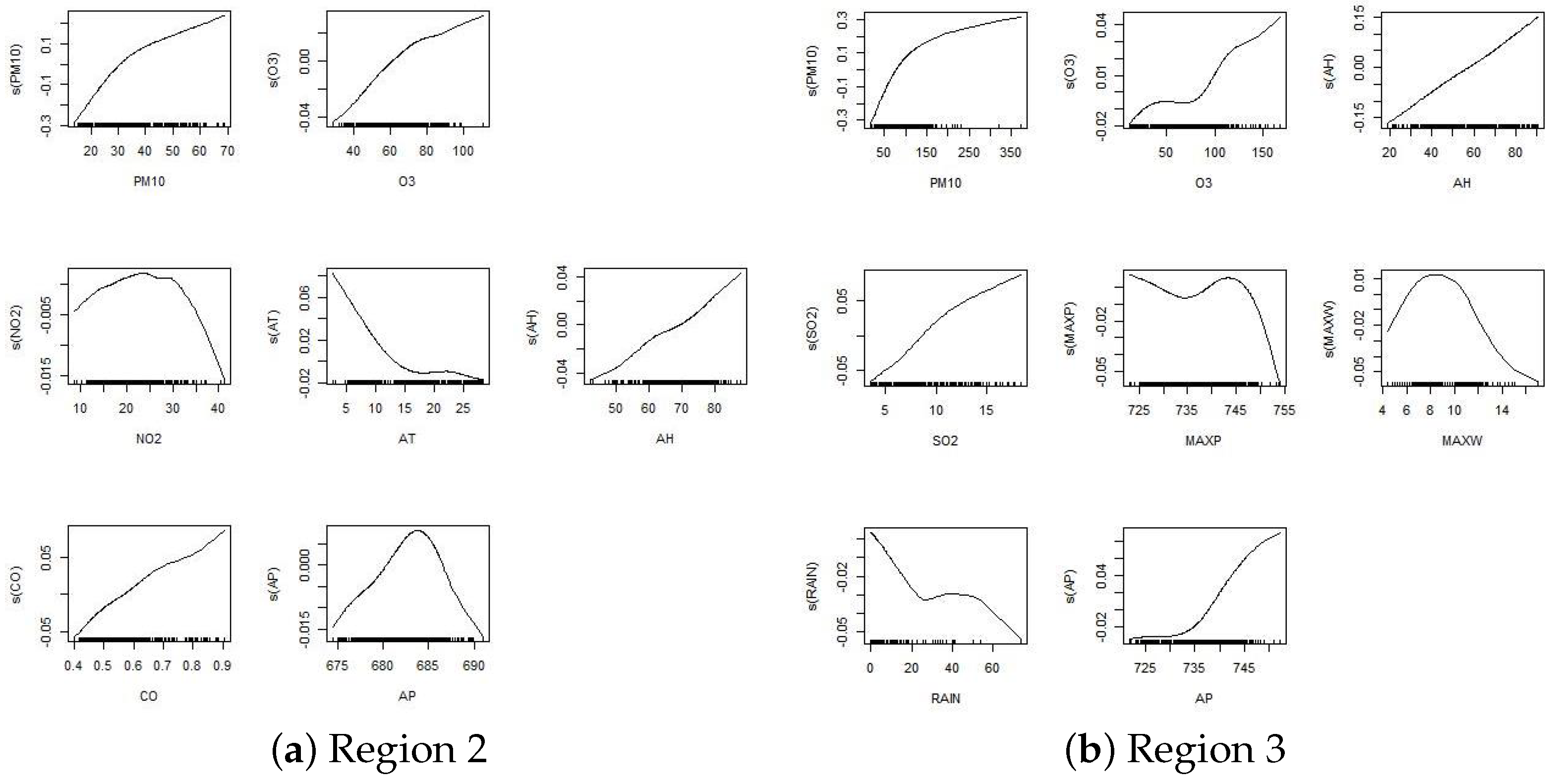
As shown in Figure 6 and

Table 7. The effect of input variables in Region 2 and Region 3 on response variable.

Region	Input Variables Effect
Region 2	PM10 Positive	O3 Positive	NO2 Complex	AT Negative	AH Positive	CO Positive	AP Complex
Region 3	PM10 Positive	O3 Positive	AH Positive	SO2 Positive	MAXW Complex	MAXP Complex	RAIN Negative	AP Positive

. In region 2, PM10, O₃, AH and CO all positively affect PM2.5 concentration, while AT has a reverse impact. With the increase of AT, the effect on PM2.5 concentration gradually slows down. When the NO₂ concentration is lower than 26 $\mathsf{\mu }\mathrm{g}/{\mathrm{m}}^3$, PM2.5 concentration rises with the increase of NO₂ concentration; when it is higher than 26 $\mathsf{\mu }\mathrm{g}/{\mathrm{m}}^3$, it reduces with the increase of NO₂ concentration. AP’s influence on PM2.5 concentration in 684 hPa begins to change. With the increase of AP, PM2.5 concentration first increases and then decreases. In region 3, PM10, AP, AH, SO₂ and O₃ all positively affect PM2.5 concentration. When the MAXW is lower than 9 m/s, the PM2.5 concentration gradually rises with the increasing MAXW; when it is higher than 9 m/s, the PM2.5 concentration declines with the increasing MAXW. The effects of MAXP and RAIN on PM2.5 concentration are more complex, and will change continuously as they rise.

See Figure 7 and

Table 8. The effect of input variables in Region 4, Region 5 and Region 7 on response variable.

Region	Input Variables Effect
Region 4	PM10 Complex	O3 Complex	SO2 Positive	AH Complex	MINP Complex
Region 5	PM10 Positive	O3 Complex	AH Positive	NO2 Positive	MINP Complex
Region 7	PM10 Positive	AP Negative	AH Positive	AT Complex	MAXW Complex	MINP Positive

. In region 4, the PM2.5 concentration increases with the SO₂ concentration. When the concentration of PM10 exceeds 170 $\mathsf{\mu }\mathrm{g}/{\mathrm{m}}^3$, its effect on PM2.5 concentration changes from positive to reverse. When AH exceeds 40%, its effect on PM2.5 concentration changes from reverse to positive. 70 $\mathsf{\mu }\mathrm{g}/{\mathrm{m}}^3$ is a turning point. With the increase of O₃ concentration, the effect on PM2.5 concentration with forward after reverse first. When MINP is lower than 730 hPa, it negatively affects on PM2.5 concentration; when MINP is higher than 730 hPa, it positively affects PM2.5 concentration. In region 5, PM10, AH and NO₂ all positively affect PM2.5 concentration. When the concentration of O₃ exceeds 110 $\mathsf{\mu }\mathrm{g}/{\mathrm{m}}^3$, its effect on PM2.5 concentration changes from reverse to positive. The effect of MINP on the concentration of PM2.5 is relatively complex, rising as MINP changes constantly, but the overall trend is positive influence on first after the reverse effect. In region 7, PM10, MINP and AH all positively affect PM2.5 concentration, while AP inversely affects PM2.5 concentration. When MAXW exceeds 14 m/s, its effect on PM2.5 concentration changes from reverse to positive. When AT is lower than −9 °C, it positively affects on PM2.5 concentration; when it is between −9 °C and 20 °C, it negatively affects PM2.5 concentration; when it is higher than 20 °C, it becomes a positive effect again.

4. Empirical Analysis of Regional and Urban PM2.5 Concentration Forecasting

In Section 3, the input variables of the model are determined by the novel PM2.5 concentration forecasting method. Section 4.1 is the empirical analysis of regional PM2.5 concentration forecasting based on the novel PM2.5 concentration forecasting method, and Section 4.2 is the comparison between the novel forecasting method and ARIMA model in forecasting urban PM2.5 concentration.

4.1. Empirical Analysis of the Novel PM2.5 Concentration Forecasting Method

Each region uses smooth spline to fit the smoothing function for the determined input variables, and also selects logarithmic connection function to build GAM based on smooth spline to forecast PM2.5 concentration in each region. The fitting effect of the training set and the prediction effect of the test set in each region are as follows.

As can be seen from Figure 8, RMSE and MAE of all regional training sets and test sets are less than 0.35 and 0.3, respectively, and MASE is less than 0.7, indicating that the fitting effect and prediction effect of the novel forecasting method are better in each region. The RMSE and MAE of the test set in each region are smaller than that of the training set, indicating that the prediction effect of all regions are better than the fitting effect. In summary, the fitting effect and prediction effect of each region are good, indicating that the new method has achieved good results in predicting regional PM2.5 concentration. Combine Figure 8 and Figure 9, the fitting effect and prediction effect of region 1 are relatively worse than those of other regions, indicating that when the new method is used to predict regional PM2.5 concentration, it is best to control the number of cities in the region within 7.

4.2. Comparison between the Novel Forecasting Method and ARIMA Model Prediction Results

According to the selection of input variables of regional PM2.5 concentration model, it can be seen that air pollutants and meteorological factors in different regions have different impacts on PM2.5 concentration. According to the regional PM2.5 concentration prediction model established above and ARIMA model, one city is selected from each region, namely Chengdu, Shanghai, Jinan, Harbin, Lanzhou, Beijing and Urumqi, and the test set data of these seven cities are used to predict urban PM2.5 concentration.

As can be seen from Figure 10, the fitting effect of the ARIMA model is general. The comparison of the prediction results of the two models is as follows. The data in

Table 9. The prediction results of the two models.

City	New Method RMSE	ARIMA RMSE	New Method MAE	ARIMA MAE	New Method MASE	ARIMA MASE
Chengdu	0.384	25.304	0.296	9.797	0.703	0.983
Shanghai	0.134	15.726	0.108	11.969	0.226	0.907
Jinan	0.140	45.661	0.110	33.205	0.177	0.983
Harbin	0.074	35.676	0.058	24.898	0.129	0.907
Lanzhou	0.106	19.530	0.082	13.560	0.286	0.983
Beijing	0.202	25.828	0.143	19.717	0.179	0.712
Urumqi	0.080	38.834	0.061	30.259	0.128	0.906

show that the prediction effect of the new method is far better than that of ARIMA model, indicating that the regional PM2.5 concentration forecasting model established according to the new method has better prediction effect. When there are more cities to forecast, using the new forecasting method is a better way. In addition, ARIMA model is suitable for short-term forecasting, and the accuracy of long-term forecasting will become worse, while the new method can objectively express the linear or nonlinear relationship between the model input variable and the response variable on the premise of ensuring the high prediction accuracy, and express the influence of the input variable on the response variable.

5. Conclusions

In this paper, a new method combining LFIG_DTW_HC algorithm and generalized additive model is proposed to analyze and predict the influencing factors of regional PM2.5 concentration. Firstly, the LFIG_DTW_HC algorithm is used to cluster according to the air quality index of each city, and descriptive statistics of PM2.5 concentration in each region are conducted. Then, the input variables of the forecasting model are determined by the method of variable correlation combined with the generalized additive model, and the regional influencing factors are analyzed. Finally, through the empirical analysis of regional forecasting, the urban predicted results based on the generalized additive model are compared with the ARIMA model, which shows that the novel PM2.5 concentration forecasting method has a better prediction effect. The next step is to consider other factors affecting PM2.5 concentration and to establish a combined forecasting method to make the prediction more accurate.