Chaotic Steady States of the Reinartz Oscillator: Mathematical Evidence and Experimental Confirmation

Abstract

This paper contributes to the problem of chaos and hyperchaos localization in the fundamental structure of analog building blocks dedicated to single-tone harmonic signal generation. This time, the known Reinartz sinusoidal oscillator is addressed, considering its conventional topology, both via numerical analysis and experiments using a flow-equivalent lumped electronic circuit. It is shown that physically reasonable values of circuit parameters can result in robust dynamical behavior characterized by a pair of positive Lyapunov exponents. Mandatory numerical results prove that discovered strange attractors exhibit all necessary fingerprints of structurally stable chaos. The new “chaotic” parameters are closely related to the standard operation of the investigated analog functional block. A few interestingly shaped, strange attractors have been captured as oscilloscope screenshots.

1. Introduction

Irregular behavior associated with analog electronic systems is caused by serious problems that have been intensively studied by engineers and researchers in the last three decades. From the viewpoint of typical properties, long-term unpredictability, broad-band frequency spectrum, and dense strange attractors are the fundamental fingerprints of chaos. Once upon a time, this kind of repeatable dynamical motion was misinterpreted as phase noise, because similar apparent properties are observed in the time and frequency domains. From the application point of view, chaotic tangles have been reported during the analysis of seemingly linear analog and digital [1] frequency filters, phase-locked loops [2], amplifiers working under different operational regimes [3], power converters [4], switched capacitor circuits [5], modulators and demodulators, mixers, very simple multi-state static memory cells [6], logic gates [7], random number generators [8], and many others. This very short and surely incomplete list implies that both autonomous and driven dynamical systems are subject to chaotic behavior; only the presence of at least one nonlinearity is mandatory.

Since the practical designs of sinusoidal oscillators require a mechanism for amplitude stabilization, these common building blocks should be treated as nonlinear. Therefore, the existence of chaos within circuit models as well as practical realizations is not a surprise. The chaotic motion is often excited by the unstable fixed points, i.e., generated strange orbits, which are members of the so-called self-exited attractors. Because of the simultaneous acting exponential divergency of state space neighboring orbits and the attractor boundedness within a finite state space volume, the minimum number of working accumulation elements is three, regardless of the combination of circuit elements. The famous Colpitts oscillator probably represents the oldest topology where chaos has been confirmed, both numerically and experimentally [9]. This kind of circuit modified to operate in the higher frequency band is addressed in paper [10]. It is shown that the parasitic base-emitter capacitance of a bipolar transistor should be a working accumulation element as well. The basic circuit structure of Hartley oscillators and chaos evolution are discussed in the framework of papers [11,12]. For nonlinear sinusoidal oscillators that have four accumulation elements, both chaos and hyperchaos represent a possible time-domain solution, as mentioned in work [13]. Also, RC feedback oscillators have been studied with respect to the generation of robust chaotic waveforms. The existence of such steady states has been observed in Wien bridge-based feedback [14], phase shift type of feedback loop [15], and atypical but very simple feedback, as suggested in paper [16]. Interesting lumped chaotic oscillators having one or two transistors and packs of surrounding passive components can be found in research paper [17]. There, authors use a heuristic approach to develop many canonical circuits with experimentally measurable, structurally stable, chaotic self-oscillations. It is shown that the natural nonlinear features of used transistors can perform folding and stretching of vector field quite easily.

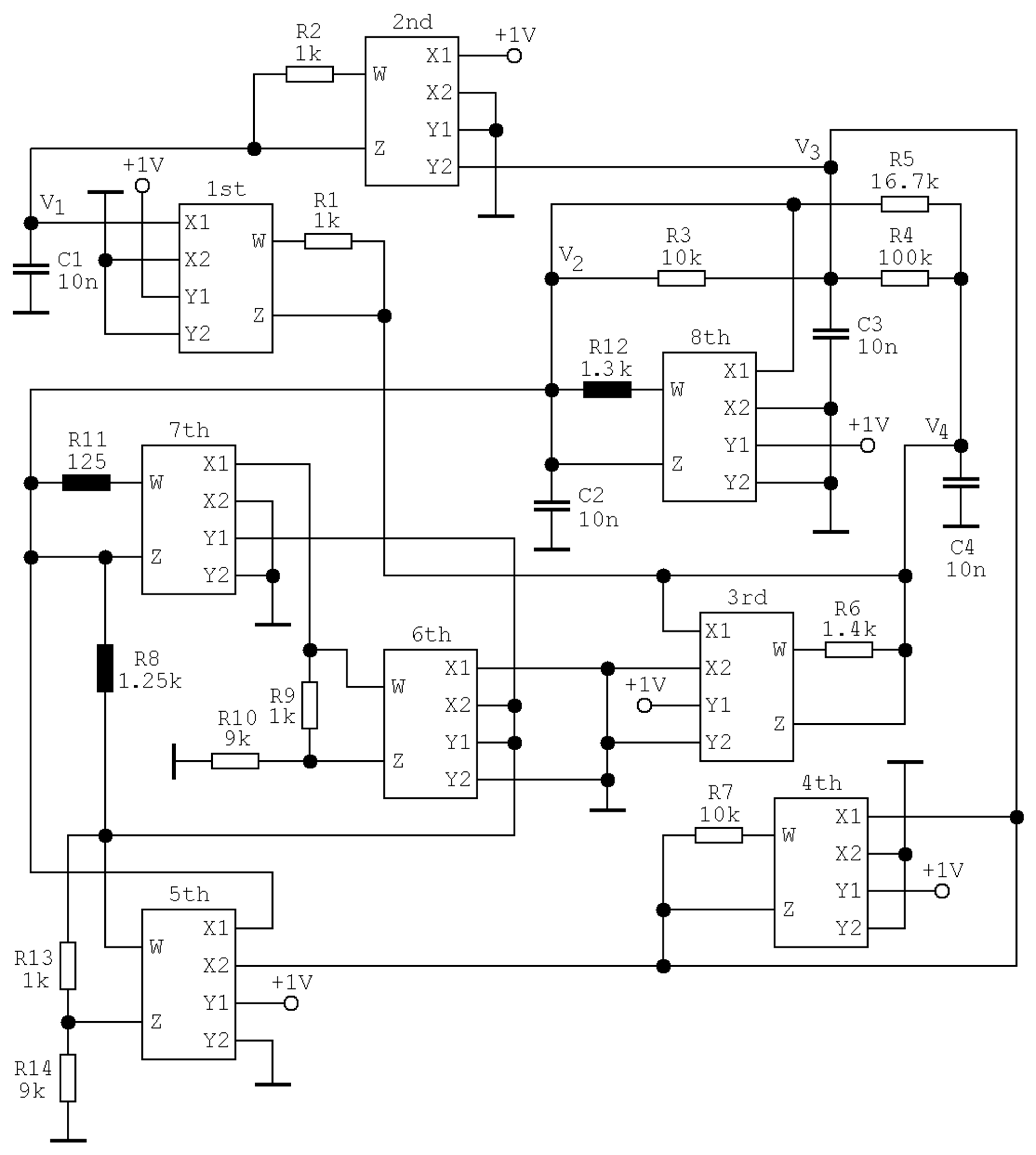
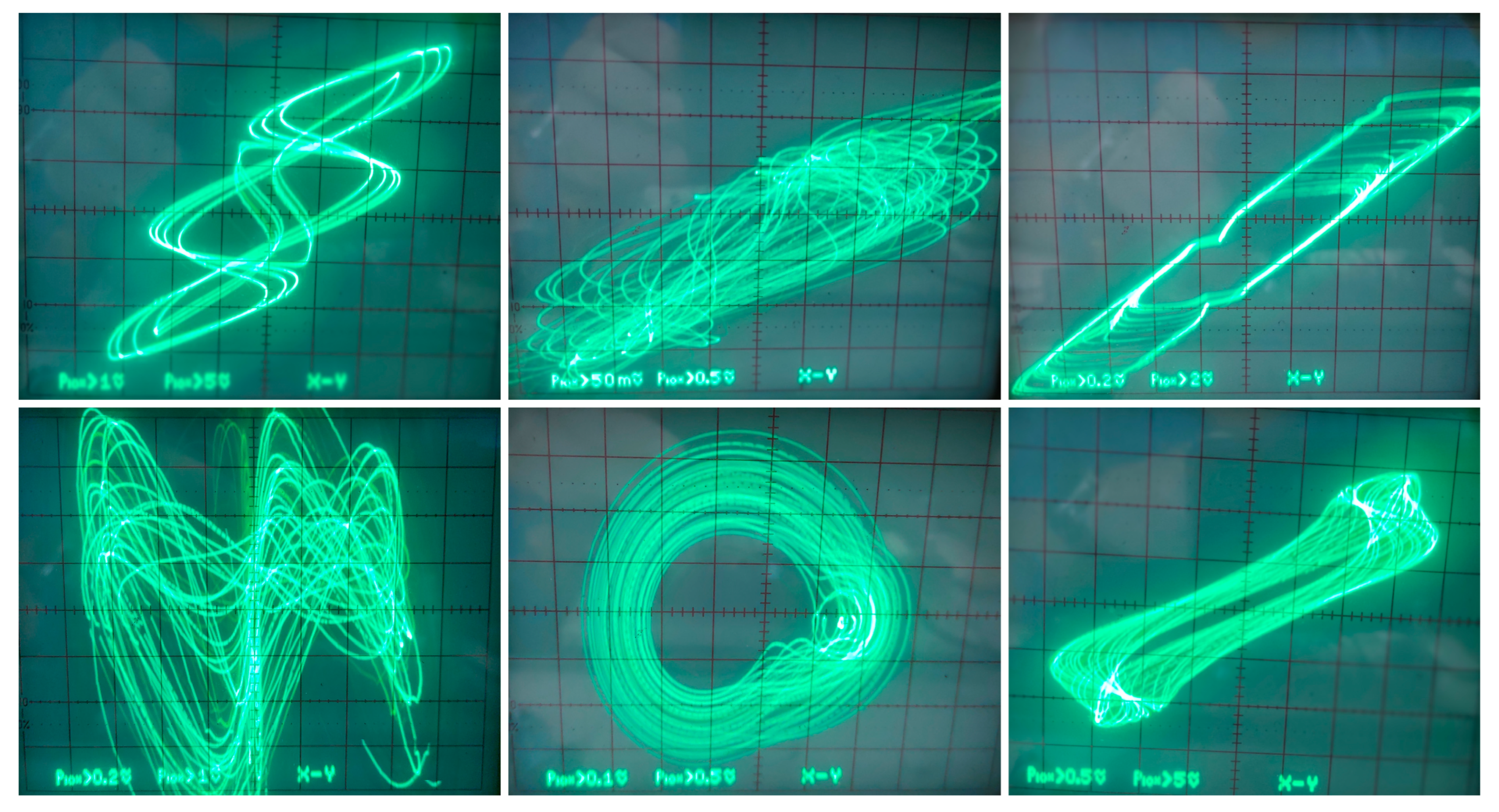
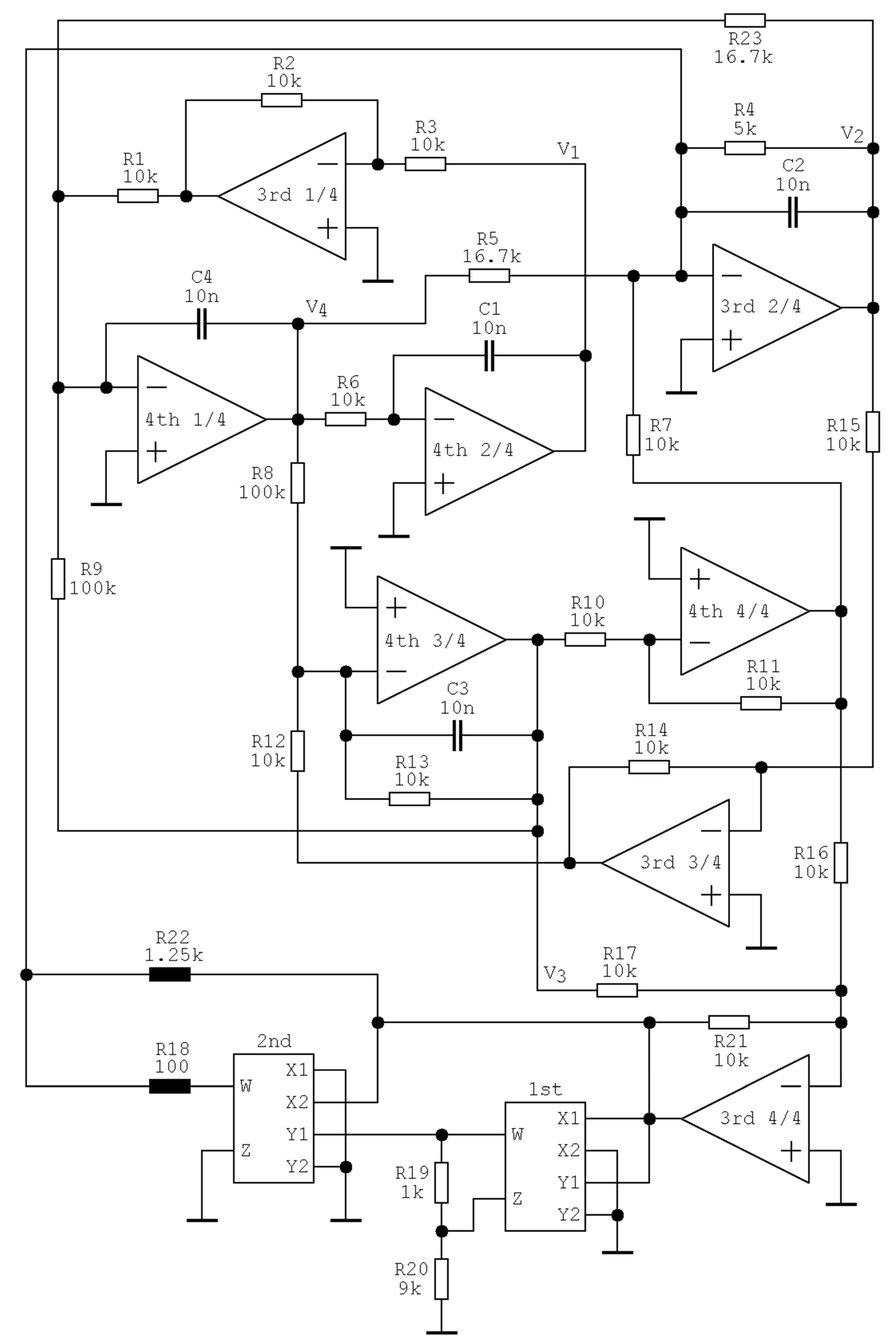
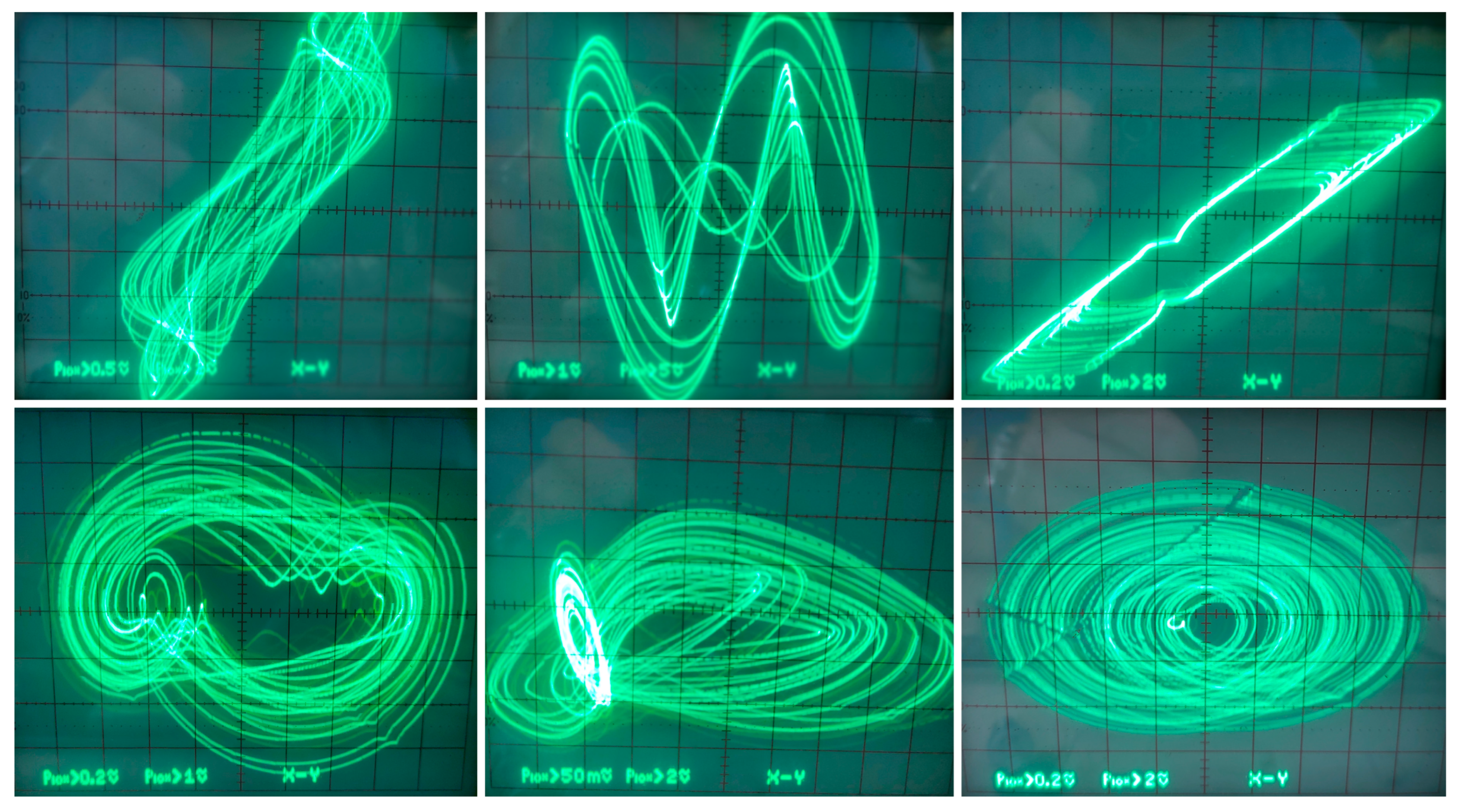
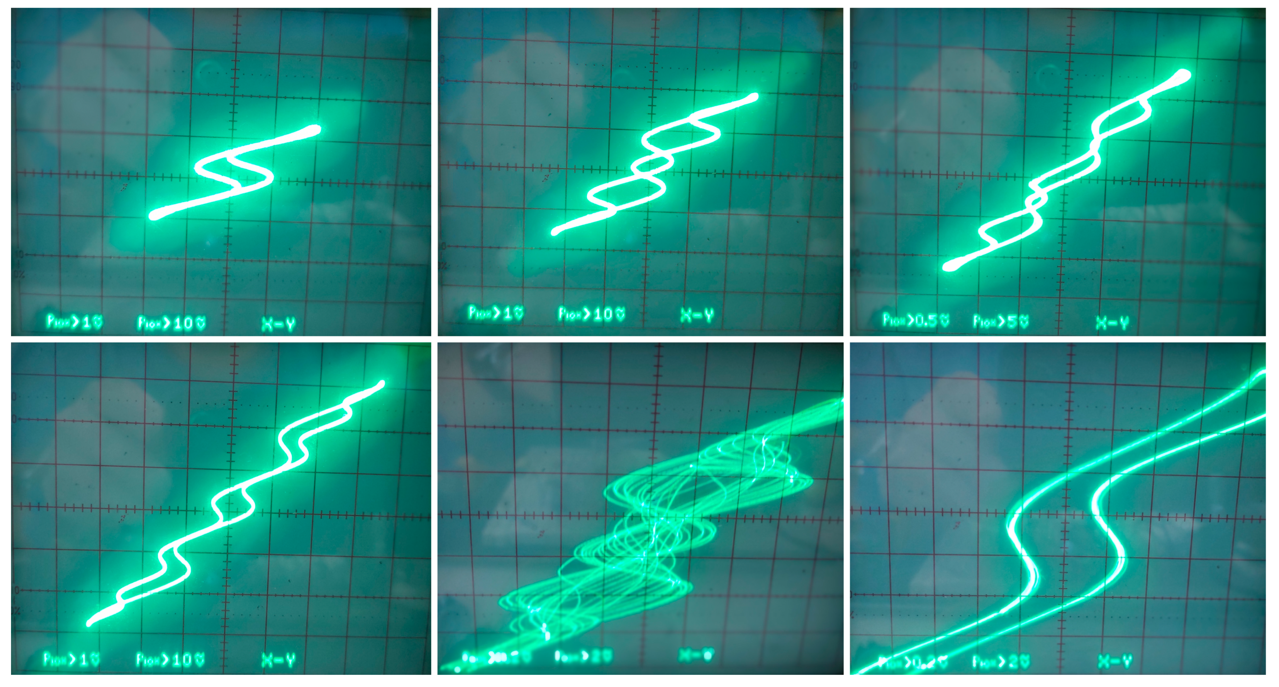
This paper is organized as follows: The next section describes a path leading to a mathematical model dedicated to numerical analysis, which is the content of the third paper section. The fourth part brings experimental verification, i.e., the construction of a flow-equivalent dynamical system based on the following two different but universal methods. Commercially available active devices are used for the realization of both the linear and nonlinear parts of the vector field. Captured oscilloscope screenshots prove that the observed chaotic behavior is neither a numerical artifact nor a long transient.

2. Mathematical Model of Reinartz Oscillator

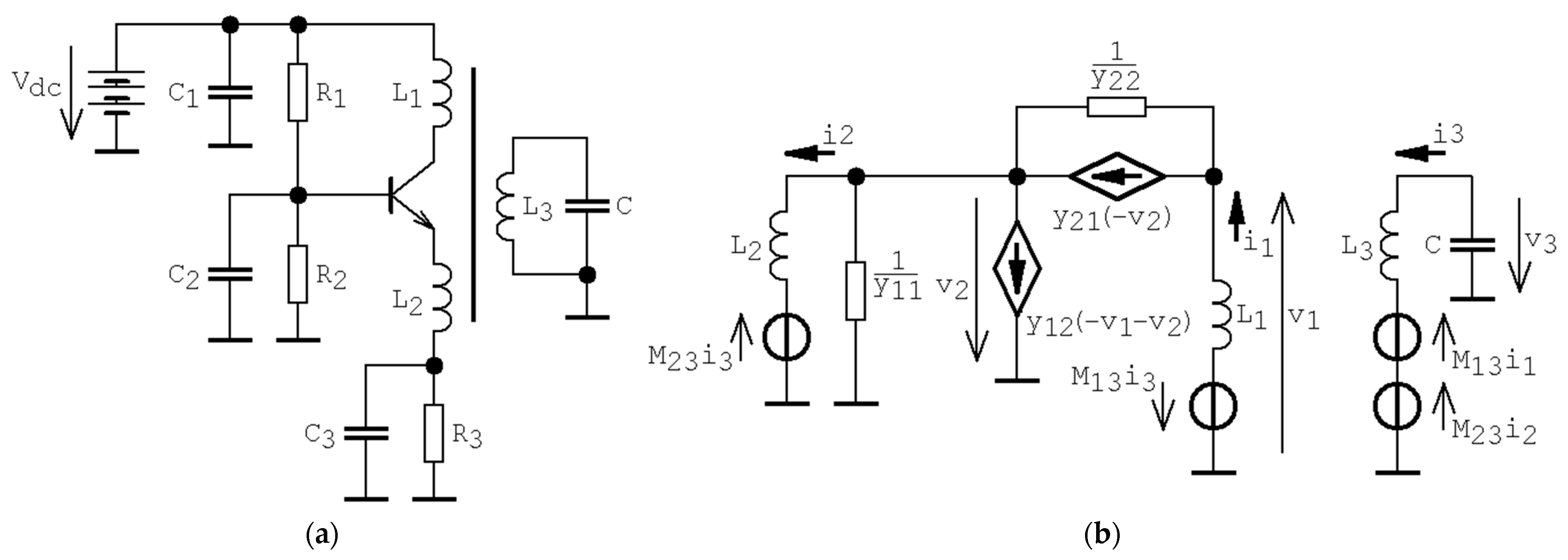
Figure 1a illustrates a circuit topology that is ready for harmonic signal generation, namely, the well-known Reinartz oscillator. This circuit typically produces low-distortion sinusoidal waveforms within a frequency band of about hundreds of kHz, typically up to units of MHz. Of course, the topology can differ slightly for specific applications.

In fact, all resistors are used to set up a bias point of a bipolar transistor, while capacitors C₁, C₂, and C₃ serve for filtering, DC blocking, and temperature drift stabilization of a bias point. Thus, an equivalent circuit for analysis in an operational frequency band can be obtained by shorting the capacitors mentioned above, causing the removal of all resistors. The hypothetical bias point of a generic bipolar transistor will be represented by a conventional two-port network described using four frequency-independent admittance parameters. The input and output admittances will be exclusively positive real numbers. Moreover, we will consider odd-symmetrical cubic polynomial forward transconductance and zero backward transconductance. Investigated autonomous lumped electronic system exploits inductively coupled emitter and collector windings to the main tank circuit formed by passive components L₃ and C. However, to avoid unwanted parasitic oscillations, inductors L₁ and L₂ are not coupled to each other.

Of course, small signal models of bipolar transistors allow us to perform a linear analysis, leading to symbolic formulas for oscillation frequency in the case that the electronic system works just on the boundary of stability. Generally, the characteristic equation will be a fourth-order polynomial with relatively complicated nonzero coefficients. However, a straightforward analysis for a complex frequency jω combined with a few justified simplifications leads to the formula for oscillation frequency $f_{osc}={\left(2\pi \sqrt{L_{3}C}\right)}^{-1}$.

In linear dynamical systems, chaotic behavior is out of the question. Nevertheless, a bipolar transistor is a nonlinear active element if a large signal must be processed. The dynamical behavior of the circuit given in Figure 1b is uniquely determined by following the set of first-order ordinary differential equations (ODEs)

$$\begin{gathered} \frac{d}{dt}{v}_3=-\frac{i_3}{C}, \frac{d}{dt}{i}_1=\frac{1}{L_1}\left[M_{13}\cdot i_3-\frac{i_1}{y_{22}}-\frac{i_1-i_2}{y_{11}}+\frac{1}{y_{22}}{y}_{21}\left(\frac{i_1-i_2}{y_{11}}\right)\right], \\ \frac{d}{dt}{i}_2=\frac{1}{L_2}\left[\frac{i_1-i_2}{y_{11}}+M_{23}\cdot i_3\right],\frac{d}{dt}{i}_3=\frac{1}{L_3}\left(v_3+M_{13}\cdot i_1+M_{23}\cdot i_2\right), \end{gathered}$$

(1)

where four-dimensional state space is formed by the vector of state variables x = (v₃, i₁, i₂, i₃)^T.

Note that voltage-controlled current-source y₁₂(v) = 0 S and forward trans-conductance y₂₁(v) will be a scalar nonlinear function of the form

$$y_{21}\left(v\right)=\alpha \cdot v^3+\beta \cdot v,$$

(2)

and symbols M₁₃ and M₂₃ represent the mutual inductances of three-wind loss-less transformers described by three linear differential equations Z·I = V (symmetry of impedance matrix Z along main diagonal indicates that the transformer is a reciprocal element)

$$\left(\begin{array}{ccc}{L}_1\frac{d}{dt}& 0& -M_{13}\frac{d}{dt}\\ 0& L_2\frac{d}{dt}& -M_{23}\frac{d}{dt}\\ -M_{13}\frac{d}{dt}& -M_{23}\frac{d}{dt}& L_3\frac{d}{dt}\end{array}\right)\cdot \left(\begin{array}{c}{i}_1\\ i_2\\ i_3\end{array}\right)=\left(\begin{array}{c}{v}_1\\ v_2\\ v_3\end{array}\right).$$

(3)

The shape of the cubic function (2) reflects the fact that the linear part of i_C vs. v_BE transfer characteristic is limited on one side by the region where the transistor is closed, and the other side is smoothly trimmed by the region of maximal output current.

The localization of fixed points associated with the dynamical system (1) in conjunction with (2) is very important. Regardless of the values of the system parameters, the origin of state space is always the only equilibrium. The search-for-chaos algorithm that allows us to find chaos within the Reinartz oscillator is focused on the self-excited strange attractors. In this case, the close neighborhood of origin will be unstable (saddle-spiral local geometry ℜ²⊕ℜ² is preferred) for all combinations of parameters. An absence of offset and quadratic terms in formula (2) leads to the symmetry of a vector field with respect to the origin. Also, forward trans-conductance y₂₁(v) is of saturation type, meaning that α < 0 ^ β > 0. This kind of output–input characteristic of the active element de facto represents the linear transformation of coordinates between a circuit-oriented model and a mathematical model. In other words, the bias point of a bipolar transistor is initially centered within the linear part of the i_C = f(v_BE) curve. Then, this point is shifted toward the origin of state space. The dynamical system (1) together with (2) is invariant under full linear change of the coordinates v₃→–v₃, i₁→–i₁, i₂→–i₂, and i₃→–i₃. Simultaneously, both M₁₃ and M₂₃ are the subject of physical realization constraints and will not be larger than the value of 0.6 H.

Several recent papers, for example, [18,19,20,21,22], utilize a multi-objective fitness function to find a robust chaotic motion within the lower-order deterministic dynamical systems. The proposed methods are often general, such that both autonomous and driven systems can be investigated. In our case, the same approach as proposed in [18] has been adopted, i.e., a three-step calculation toward weighted cost function. The first step covers a simple check of the stability of the fixed point located at the origin. In this stage, all sets of parameters leading to unwanted local geometry near the state space origin can be omitted early, significantly saving time demands for optimization. The second test is a calculation of attractor boundedness and dissipation of the flow. If passed, the full spectrum of Lyapunov exponents (LE) is established, and the Kaplan–Yorke dimension of the state space attractor is calculated. For chaos, the first LE needs to be positive, and the sum of all LEs must be negative. For hyperchaos, there is a pair of two significantly positive Les, while the sum of all LEs stands negative. Within each optimization step, the numerical values of all system parameters (defined up to two decimal places) are known. Thus, corresponding eigenvalues associated with a fixed point at the origin can be easily obtained, and an optimal time step size for numerical calculations can be determined and updated accordingly; check paper [23] for more details. Note that the calculations of individual cost functions are independent; the sets of system parameters are exclusive input variables. Therefore, a search-for-chaos routine is a good candidate for multi-core parallel processing.

Thanks to impedance and time scaling, working accumulation elements can be kept in unity, i.e., L₃ = 1 H and C = 1 F, such that the fundamental frequency component equals 159 mHz. The common operational regime deals with the ratio L₁/L₂→10. In an upcoming analysis, we suppose unity inductances L₁ = L₂ = 1 H to unify the time constants associated with individual differential equations. From the viewpoint of watched dynamical system properties, the existence of long-term structurally stable strange attractors is conditioned by the flow dissipation, that is

$$\begin{gathered} \mathbf{x}\in \mathsf{\varphi }\left(t\right):\mathrm{div}\left(\mathbf{F}\right)=\frac{\partial }{\partial v_3}{\mathbf{F}}_1+\frac{\partial }{\partial i_1}{\mathbf{F}}_2+\frac{\partial }{\partial i_2}{\mathbf{F}}_3+\frac{\partial }{\partial i_3}{\mathbf{F}}_4= \\ \frac{1}{L_1\cdot y_{11}^3\cdot y_{22}}\left[3\cdot \alpha \cdot \left(i_1^2+i_2^2\right)-6\cdot \alpha \cdot i_1\cdot i_2\right.\left.+y_{11}^2\left(\beta -y_{22}-y_{11}\right)\right]-\frac{1}{L_2\cdot y_{11}} , \end{gathered}$$

(4)

where ϕ(t) represents a state orbit, F means a four-dimensional vector field, and F_k is the right-hand side of k-th ODE. In both cases of investigated chaotic systems (will be revealed below), this function stands negative (in average) for complete ranges of state variables i₁ and i₂ of a fully evolved strange attractor. Another key property of the final dynamical system is the existence of an unstable fixed point located at the origin. This requirement means that the characteristic polynomial

$$\begin{array}{c}{\lambda }^4+\frac{2\cdot y_{11}+y_{22}-\beta }{y_{11}\cdot y_{22}}{\lambda }^3+\frac{y_{11}^2\cdot y_{22}^2\left(1-M_{13}^2-M_{23}^2\right)+y_{11}\left(y_{22}-\beta \right)-y_{22}\left(y_{22}-\beta \right)}{y_{11}^2\cdot y_{22}^2}{\lambda }^2+\\ \frac{y_{11}\left(2-M_{13}^2-M_{23}^2\right)-\beta +y_{22}+M_{23}^2\left(\beta +y_{22}\right)-M_{13}\cdot M_{23}\left(2\cdot y_{22}-\beta \right)}{y_{11}\cdot y_{22}}\lambda +\frac{y_{11}^2+y_{11}\cdot y_{22}-y_{22}^2+\beta \left(y_{22}-y_{11}\right)}{y_{11}^2\cdot y_{22}^2}=0,\end{array}$$

(5)

has at least one root with positive real parts. Assume a limited case of zero coupling between windings, i.e., M₁₃ = 0 H and M₂₃ = 0 H. Solving for the roots of polynomial (5) gives us information about the oscillating solution of isolated L₃C tanks and the stability of the rest of the circuit, namely

$${\lambda }_{\mathrm{1,2}}=\pm j,{\lambda }_{\mathrm{3,4}}=\pm \frac{\sqrt{\left(\beta -y_{22}\right)\cdot \left(\beta -5\cdot y_{22}\right)}}{2\cdot y_{11}\cdot y_{22}}-\frac{2\cdot y_{11}^2\cdot y_{22}+y_{11}\cdot y_{22}^2-\beta \cdot y_{11}\cdot y_{22}}{2\cdot y_{11}^2\cdot y_{22}^2}.$$

(6)

The eigenvalues λ_3,4 can be of any conceivable configuration depending on the relations between y₁₁, y₂₂, and β. This includes eigenvalues that are both real and negative, real with opposite signs, real eigenvalues with positive parts, and complex conjugated numbers with either positive or negative real parts. Obviously, both the input and output admittance of transistors cannot be zero. Important bifurcation planes are given by β = y₂₂ and β = 5·y₂₂ since the third and fourth eigenvalues form a complex conjugated pair between these lines. It is worth mentioning that each change in the vector field geometry near the state space origin is followed by a dramatic change in the global system dynamics. During intensive numerical analysis (especially using the searching for chaos routine), it finally turns out that at least one stable manifold associated with state space origin is needed for chaos and/or hyperchaos evolution. Of course, the existence of unpredictable behavior in the case of full repelor at the origin of state space is not definitely excluded, and it can be considered a possible topic for future investigations.

In the upcoming section of this paper, the results originating from the application of such a brute-force numerical search algorithm applied on basic AC-ready circuit topology of a Reinartz oscillator are provided. Proposed optimization/search routine was implemented in Matlab and can be adopted (with small adaptation changes) for any type of finite-order dynamical system, including those with fractional-order derivations of some state variable. However, the huge number of required numerical operations makes it usable only if appropriate computing power is available. In the case of this work, a workstation composed of i9-10900K (3.7 GHz) and 128 GB RAM was utilized.

3. Numerical Analysis and Results

A mathematical model dedicated to numerical analysis and optimization will be considered dimensionless and expressed in the form of system (1) with nonlinear features of transistor (2), and with {M₁₃, M₂₃, y₁₁, y₂₂, α, β} being a group of unknowns. Within the optimization procedure, the value of each unknown is encoded into a binary expression; the sought parameters can take non-extreme, physically reasonable discrete values only. Two decimal places represent a smooth-enough resolution.

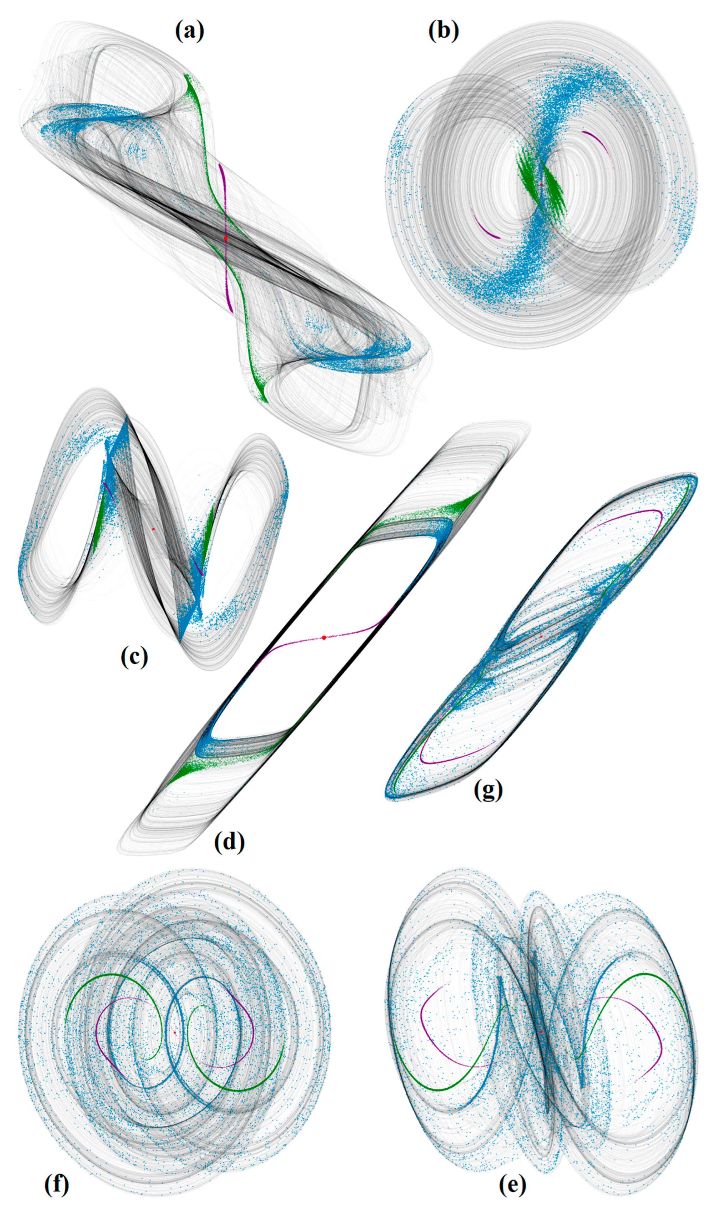
Two distinct sets of parameters that lead to the topologically similar, robust, and chaotic behavior were discovered. Concretely, the first set (case I) is

$$M_{13}=0.6H,M_{23}=0.1H,y_{11}=1S,y_{22}=1S,\alpha =-8A\cdot V^{-3},\beta =10S.$$

(7)

while the second set (case II) is

$$M_{13}=0.52H,M_{23}=0.22H,y_{11}=2S,y_{22}=4S,\alpha =-8A\cdot V^{-3},\beta =18S.$$

(8)

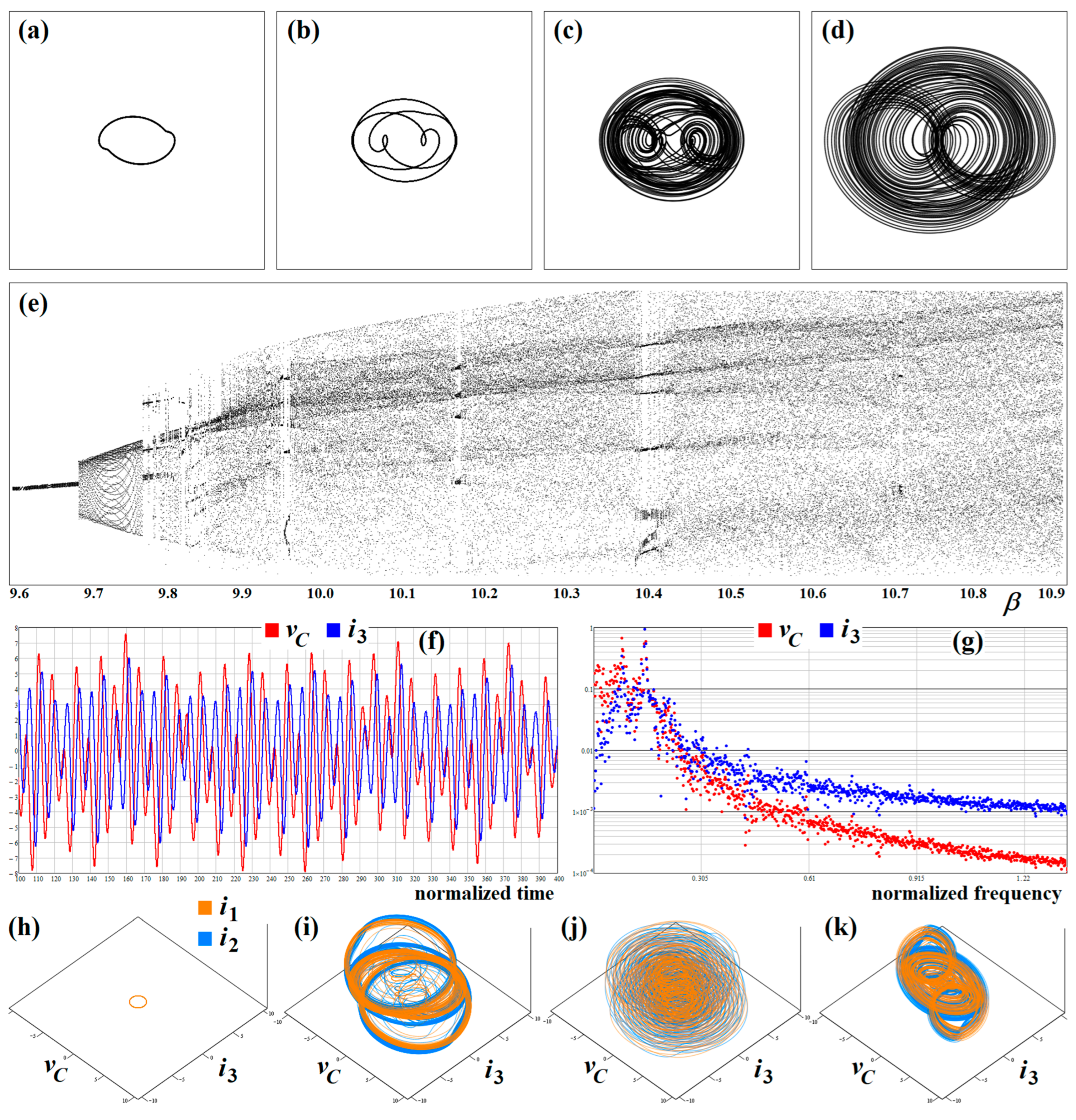
Figure 2 shows both the geometrical shape of a chaotic attractor and the sensitivity dependance on the tiny changes in the initial conditions. For each case mentioned above, a group of 10⁴ initial conditions was generated randomly around the state space origin with a normal distribution and standard deviation 10^–2 (red dots). Then, the final states after short-term (t_max = 10 s, purple points), average-term (t_max = 50 s, green points), and long-term (t_max = 100 s, blue points) evolution are stored and visualized. For all simulations, the fourth-order Runge–Kutta integration method was utilized with a fixed time step of 100 μs.

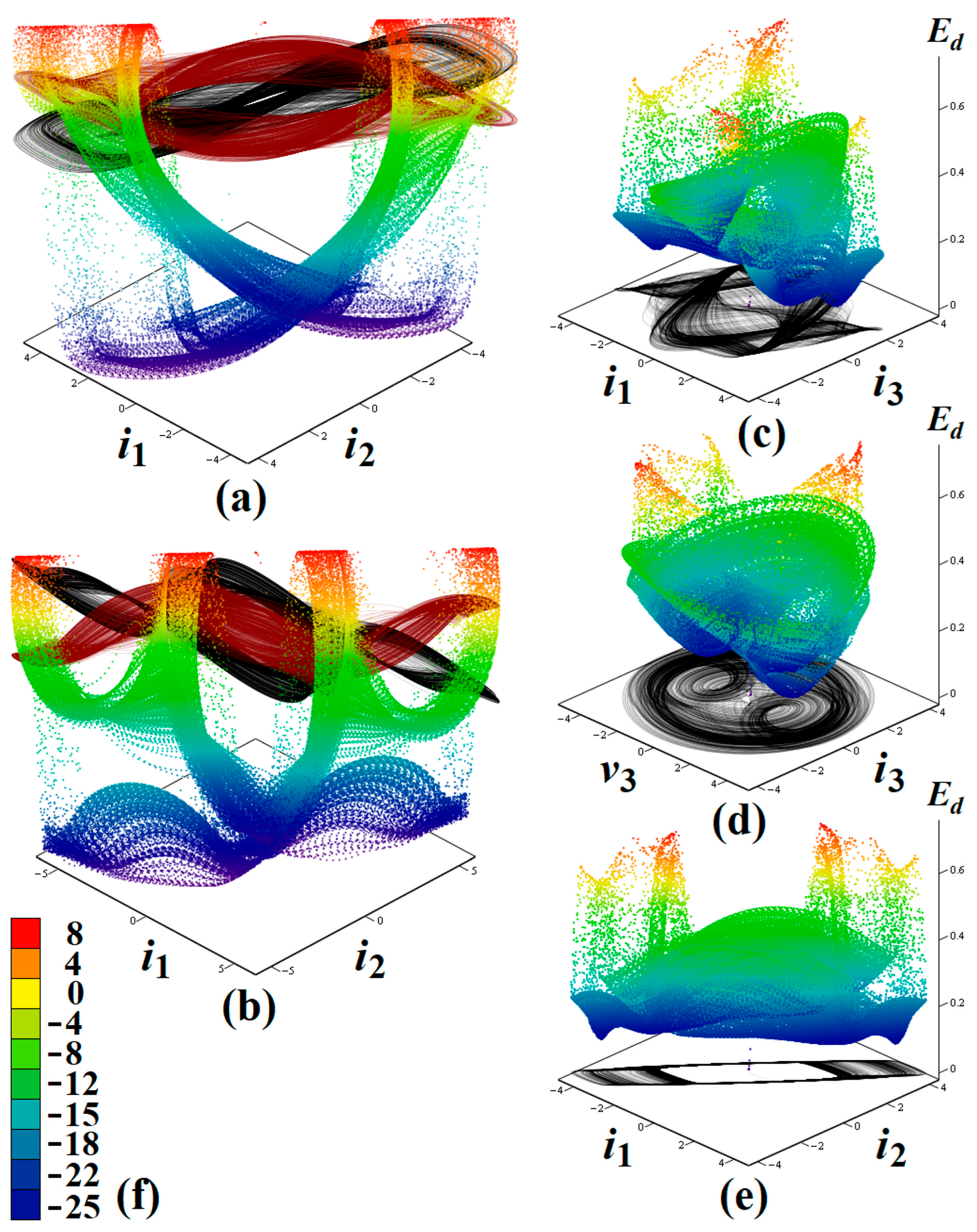
Figure 3 contains interesting numerical results concerning the Reinartz oscillator, case I. Firstly, plots showing the divergency of the vector field along a chaotic orbit can be found there. A typical strange attractor (for β = 10 S and β = 11 S) is located within the state space volume with very small positive values and a negative value close to zero. Figure 3 also provides the distribution of dynamic energy along the trajectory associated with parameter set (7). Note that all mutual inductances M₁₃ and M₂₃ for dynamical system case I and II represent tight coupling between primary and secondary windings. For both cases of chaotic systems, the origin is an unstable equilibrium point, as monitored frequently during the search-for-chaos optimization procedure. For parameter set (7), zero equilibrium exhibits a stable two-dimensional manifold, and the corresponding eigenvalues are

$${\lambda }_1=6.904,{\lambda }_2=0.149,{\lambda }_{\mathrm{3,4}}=-0.026\pm j0.985.$$

(9)

In comparison with these results, parameter set (8) leads to the following eigenvalues:

$${\lambda }_{\mathrm{1,2}}=-0.089\pm j0.915,{\lambda }_{\mathrm{3,4}}=0.714\pm j0.285.$$

(10)

Because of different vector field geometry near the 4D state space origin, self-excited chaotic attractors discovered by searching routine can be marked as distinct types.

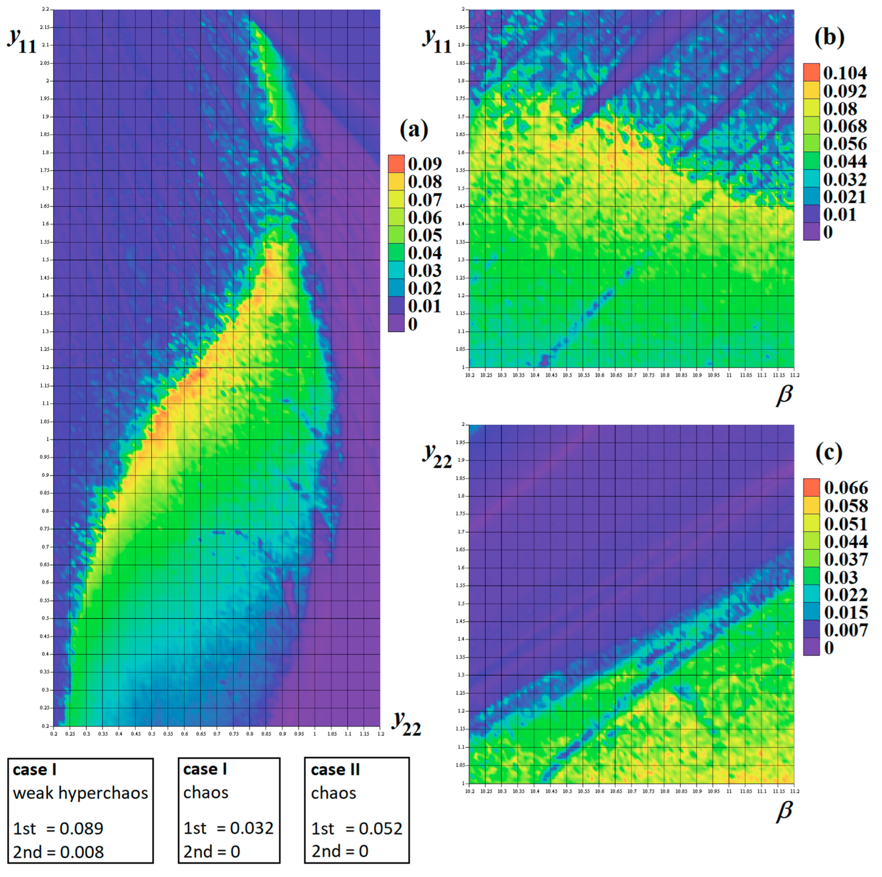
Figure 4 provides a closer insight into how regions of chaos (of course, only a small fragment is addressed) within a hyperspace of system parameters look. These are high-resolution plots with a total number of calculated values of 50 × 50 = 2500 in each square. Transitions between chaotic and hyperchaotic behavior do not follow conventional rules such as changes in eigenvalues or the stability index of zero equilibrium; see paper [24] for more details. Little can be known about these routes, only that they are rare and cannot be described by a closed-form mathematical formula.

Figure 5 provides a continuation of numerical results, showing time-domain analysis results for the Reinartz oscillator (1) coupled with a parameter set (7). The bifurcation diagram reveals a sudden transition from periodic to chaotic motion and several narrow periodic windows for continuous change in the parameter β from 9.5 S up to 10.9 S. This bifurcation sequence ends up with an unbounded solution. For all numerical integrations, the initial conditions were chosen as small disturbances (100 mV) of capacitor voltage.

4. Design of Chaotic Oscillators and Experiments

Since fully analog circuit-aided solutions of ODE sets are free of numerical errors, a truly chaotic steady state can be distinguished from a long chaotic transient or numerical artifact. For further reading about the credibility aspects of research focused on chaotic dynamical systems, papers [25,26] are recommended.

Modeling nonlinear dynamics using analog circuits is a well-established task, with multiple correct solutions achieved by the following different approaches. The main goal is to reach one-to-one correspondence between the behavior of the mathematical and circuit models of the dynamical system. The complete framework on how to proceed is outlined in the comprehensive review paper [27] for voltage-mode networks and in paper [28] for current-mode operation regimes.

In the upcoming subsections, two universal methods dedicated to nonlinear circuit synthesis of flow-equivalent, case I, chaotic Reinartz oscillator are given, including the numerical values of all passive components. By considering the dynamical system (1) with nonlinearity (2) and the discovered parameters (7), the normalized (with respect to time and impedance) set of the ODE becomes

$$\begin{gathered} \frac{d}{dt}{v}_1=-v_4,\frac{d}{dt}{v}_2=0.6\cdot v_4-2\cdot v_2+v_3-8\cdot \left(v_2-v_3\right)+10\cdot {\left(v_2-v_3\right)}^3,\frac{d}{dt}{v}_3=v_2-v_3+0.1\cdot v_4, \\ \frac{d}{dt}{v}_4=v_1+0.6\cdot v_2+0.1\cdot v_3, \end{gathered}$$

(11)

where x = (v₁, v₂, v₃, v₄)^T is a new state vector composed of node voltages only. Parameters α and β need to be separated because they will be considered the variables. The circuit design of system case II is completely analogical; no changes in the circuit element’s inter-connections are necessary. It is worth nothing that the Orcad Pspice circuit simulations lead to the same results as real experimental observations captured by an oscilloscope. Hence, these results are not provided.

4.1. Analog Multiplier-Based Design

For the generation of any type of attractors, continuous offset voltage applied to the inputs of operational amplifier-based ideal integrators can be problematic simply because of the output saturation. This event can also be caused by the intrinsic nonideal offset voltage of an operational amplifier. In such cases, the classical approach, where the right-hand side of each equation of system (1) represents a sum of the currents flowing through a grounded capacitor, will probably be the better design approach. To minimize the final number of active elements, the linear part of the vector field should be decomposed: in part Y_passive, which contains grounded and passive resistors and in part Y_active where individual entries are implemented using active transadmittance cells. Then, the final matrix equations will be

$$\frac{d}{dt}{\left(\begin{array}{cc}{C}_1& \begin{array}{ccc}{C}_2& C_3& C_4\end{array}\end{array}\right)}^{\mathrm{T}}=\left({\mathbf{Y}}_{\mathit{passive}}+{\mathbf{Y}}_{\mathit{active}}\right)\cdot \mathbf{V}+\mathbf{f}\left(\mathbf{V}\right),$$

(12)

where V is a vector of the main node voltages and f comprises nonlinear functions. For the dynamical system (11), the matrices and vectors mentioned above can be of the form

$${\mathbf{Y}}_{\mathit{passive}}=\left(\begin{array}{cccc}0& 0& 0& 0\\ 0& -9.6& 1& 0.6\\ 0& 1& -1.1& 0.1\\ 0& 0.6& 0.1& -0.7\end{array}\right),{\mathbf{Y}}_{\mathit{active}}=\left(\begin{array}{cccc}0& 0& 0& -1\\ 0& 7.6& 0& 0\\ 0& 0& 0.1& 0\\ 1& 0& 0& 0.7\end{array}\right),\mathbf{f}=\left(\begin{array}{c}0\\ -8\cdot \left(v_2-v_3\right)+10\cdot {\left(v_2-v_3\right)}^3\\ 0\\ 0\end{array}\right).$$

(13)

A corresponding chaotic oscillator is provided in Figure 6. There, resistors and capacitors have fixed values derived from the basic time constants of integrators chosen quite large, namely τ = R_nom·C = 10⁴·10^–8 = 100 μs. The corresponding sets of ODEs are

$$\begin{gathered} C_1\frac{d}{dt}{v}_1=-\frac{K_2}{R_2}{v}_4,C_2\frac{d}{dt}{v}_2=\left(\frac{K_8}{R_{12}}-\frac{1}{R_3}-\frac{1}{R_5}-\frac{1}{R_8}\right)v_2+\frac{1}{R_3}{v}_3+{\frac{1}{R_5}v}_4+\frac{1}{R_8}\left(v_2-v_3\right)-\frac{K_7}{R_{11}}{\left(v_2-v_3\right)}^3, \\ {C}_3\frac{d}{dt}{v}_3=\frac{1}{R_3}{v}_2+\left(\frac{K_4}{R_7}-\frac{1}{R_3}-\frac{1}{R_4}\right)v_3+\frac{1}{R_4}{v}_4,C_4\frac{d}{dt}{v}_4=\frac{K_1}{R_1}{v}_1+\frac{1}{R_5}{v}_2+\frac{1}{R_4}{v}_3+\left(\frac{K_3}{R_6}-\frac{1}{R_4}-\frac{1}{R_5}\right)v_4. \end{gathered}$$

(14)

For derivation of these ODEs, an ideal transfer function of analog multipliers has been used, i.e., V_W = K·(V_X1–V_X2)·(V_Y1–V_Y2) + V_Z, where K = 0.1 is an internally trimmed constant. Obviously, entries of the admittance matrix Y_active can be changed via external DC voltage; in our design case, we chose default 1 V for simplicity. The chaotic system working in a lower frequency band is well suited for a breadboard realization. Resistors R₉ and R₁₀ do not appear in (14) since these serve only to compensate for constant K₆. Similarly, components R₁₃ and R₁₄ are dedicated to the compensation of constant K₅. To continuously trace some routing-to-chaos bifurcation scenarios, a nonlinear shape of forward transconductance is supposed to be independently variable. System parameter β can be changed via variable resistor R₈, and resistor R₁₁ directly adjusts the cubic term of polynomial (2), parameter α. The actual value of R₁₂ needs to be adjusted accordingly to R₈. Several examples of oscilloscope screenshots captured during experimental verification of this novel chaotic oscillator are provided in Figure 7.

4.2. Integrator Block Schematic-Based Design

Obviously, a design concept based strictly on analog multiplies requires a total of eight integrated circuits. As we will see, the total number of active elements is twofold if compared to the design approach based on the integrator block schematic. A chaotic oscillator equivalent to the same Reinartz oscillator was successfully implemented and verified using four integrated circuits only (a pair of voltage feedback operational amplifiers TL084, two analog multipliers AD633). Because of the zero mean of generated chaotic waveforms (full symmetry of the desired strange attractors), integrator-based circuit synthesis is possible. The final circuit is shown in Figure 8. Its behavior is determined by the following ODE:

$$\begin{gathered} C_1\frac{d}{dt}{v}_1=-\frac{v_4}{R_6},C_2\frac{d}{dt}{v}_2=-\frac{v_2}{R_4}+\frac{R_{11}{v}_3}{{R_{7}R}_{10}}-\frac{v_4}{R_5}+\frac{R_{21}}{R_{22}}\left(\frac{v_3}{R_{17}}-\frac{R_{11}}{R_{10}}\cdot \frac{v_2}{R_{16}}\right)-\frac{R_{21}}{R_{18}}{\left(\frac{v_3}{R_{17}}-\frac{R_{11}}{R_{10}}\cdot \frac{v_2}{R_{16}}\right)}^3, \\ {C}_3\frac{d}{dt}{v}_3=\frac{R_{14}{v}_2}{R_{12}{R}_{15}}-\frac{v_3}{R_{13}}-\frac{v_4}{R_8},C_4\frac{d}{dt}{v}_4=\frac{R_2{v}_1}{R_1{R}_3}+\frac{v_2}{R_{23}}-\frac{v_3}{R_9}. \end{gathered}$$

(15)

Resistors R₁₉ and R₂₀ do not take part in this set of equations since these components serve to annulate coefficient K₁. Systems (15) and (11) are related via a simple linear transformation of state space coordinates v₁→–v₁ and –v₄→–v₄. A few pieces of true experimental verification of the designed chaotic oscillator are provided in Figure 9 and Figure 10. In the latter case, a sequence of limit cycles that is shortly interrupted by a chaotic attractor is demonstrated for continuously increased values of parameter β.

5. Discussion

The main aim and importance of this work is to demonstrate the existence of robust, non-predictable waveforms coming from a significantly simplified mathematical model of a conventional LC oscillator. The investigated mathematical model includes only a single scalar nonlinear function intrinsic to the bipolar transistor instead of dealing with an enormously complicated large-signal global model of this three-terminal device. The presented results can motivate other design engineers and mathematicians to follow this research and extend it by including the following:

• Findings from the area of non-integer order dynamics associated with individual accumulation elements [29,30].
• Discoveries from higher-order dynamics that originate in considering parasitic properties of transistors [31].
• A description of circuit behavior under nonlinear magnetic coupling that is closer to practical reality [32].

6. Conclusions

The simplified topology of the well-known Reinartz circuit can produce either chaotic or weakly hyperchaotic self-oscillations, even under conditions of linear magnetic coupling coefficients. Proof is demonstrated within this study on both a numerical and an experimental basis. A bipolar transistor is modeled by two-port admittance parameters with the assumption of neutralized backward signal transmission. The bias point of the transistor is derived from a class A amplifier. Although biasing is hypothetical, parameter sets that result in observed chaotic steady states represent physically reasonable quantities (after suitable time and impedance rescaling) not far away from common numerical values. In accordance with explicit model vs. circuit parameter comparison and visual observation, very good agreement between measurement results and theoretical assumptions has been achieved.

References

1. Jiang, T.; Wang, B.; Bi, M.; Chen, X.; Cheng, S.; Wang, F. Digital filter based on chaos theory used for removing narrow-frequency-band noise in PD signals. J. Eng. 2020, 13, 357–360. [Google Scholar] [CrossRef]
2. Endo, T.; Chua, L.O. Chaos from phase-locked loops. IEEE Trans. Circuits Syst. 1988, 35, 987–1003. [Google Scholar] [CrossRef]
3. Petrzela, J. Generalized single stage class C amplifier: Analysis from the viewpoint of chaotic behavior. Appl. Sci. 2020, 10, 5025. [Google Scholar] [CrossRef]
4. Hamill, D.C.; Jeffries, D.J. Subharmonics and chaos in a controlled switched-mode power converter. IEEE Trans. Circuits Syst. 1988, 35, 1059–1061. [Google Scholar] [CrossRef]
5. Rodriguez-Vazquez, A.; Huertas, J.; Chua, L.O. Chaos in switched-capacitor circuit. IEEE Trans. Circuits Syst. 1985, 32, 1083–1085. [Google Scholar] [CrossRef]
6. Petrzela, J. Strange attractors generated by multiple-valued static memory cell with polynomial approximation of resonant tunneling diodes. Entropy 2018, 20, 697. [Google Scholar] [CrossRef]
7. Behnia, S.; Pazhotan, Z.; Ezzati, N.; Akhshani, A. Reconfigurable chaotic logic gates based on novel chaotic circuit. Chaos Solitons Fractals 2014, 69, 74–80. [Google Scholar] [CrossRef]
8. Drutarovsky, M.; Galajda, P. A robust chaos-based true random number generator embedded in reconfigurable switched-capacitor hardware. Radioengineering 2007, 16, 120–127. [Google Scholar]
9. Kennedy, M.P. Chaos in the Colpitts oscillator. IEEE Trans. Circuits Syst. I Fund. Theory Appl. 1994, 41, 771–774. [Google Scholar] [CrossRef]
10. Wafo Tekam, R.B.; Kengne, J.; Kenmoe, G.D. High frequency Colpitts oscillator: A simple configuration for chaos generation. Chaos Solitons Fractals 2019, 126, 351–360. [Google Scholar] [CrossRef]
11. Kvarda, P. Chaos in Hartley’s oscillator. Int. J. Bifurc. Chaos 2002, 12, 2229–2232. [Google Scholar]
12. Tchitnga, R.; Fotsin, H.B.; Nana, B.; Louodop Fotso, P.H.; Woafo, P. Hartley’s oscillator: The simplest chaotic two-component circuit. Chaos Solitons Fractals 2019, 126, 351–360. [Google Scholar] [CrossRef]
13. Petrzela, J. Chaotic and hyperchaotic dynamics of a Clapp oscillator. Mathematics 2022, 10, 1868. [Google Scholar] [CrossRef]
14. Morgul, O. Wien bridge based RC chaos generator. Electron. Lett. 1995, 31, 2058–2059. [Google Scholar] [CrossRef]
15. Hosokawa, Y.; Nishio, Y.; Ushida, A. Analysis of chaotic phenomena in two RC phase oscillators coupled by a diode. IEICE Trans. Fundam. Electron. Comm. Comput. Sci. 2001, 84, 2288–2295. [Google Scholar]
16. Bernat, P.; Balaz, I. RC autonomous circuits with chaotic behavior. Radioengineering 2002, 11, 1–5. [Google Scholar]
17. Minati, L.; Frasca, M.; Oswiecimka, P.; Faes, L.; Drozdz, S. Atypical transistor-based chaotic oscillators: Design, realization, and diversity. Chaos Interdiscip. J. Nonlinear Sci. 2017, 27, 073113. [Google Scholar] [CrossRef]
18. Petrzela, J. Chaotic states of transistor-based tuned-collector oscillator. Mathematics 2023, 11, 2213. [Google Scholar] [CrossRef]
19. Jafari, S.; Sprott, J.C.; Pham, V.-T.; Mohammad Reza Hashemi Golpayegani, S.; Jafari, A.H. A new cost function for parameter estimation of chaotic systems using return maps as fingerprints. Int. J. Bifurc. Chaos 2014, 24, 1450134. [Google Scholar] [CrossRef]
20. Petrzela, J. New chaotic dynamical system with a conic-shaped equilibrium located on the plane structure. Appl. Sci. 2017, 7, 976. [Google Scholar] [CrossRef]
21. Adeyemi, V.-A.; Tlelo-Cuautle, E.; Perez-Pinal, F.-J.; Nunez-Perez, J.-C. Optimizing the maximum Lyapunov exponent of fractional order chaotic spherical system by evolutionary algorithms. Fractal Fract. 2022, 6, 448. [Google Scholar] [CrossRef]
22. Nunez-Perez, J.-C.; Adeyemi, V.-A.; Sandoval-Ibarra, Y.; Perez-Pinal, F.-J.; Tlelo-Cuautle, E. Maximizing the chaotic behavior of fractional order Chen system by evolutionary algorithm. Mathematics 2021, 9, 1194. [Google Scholar] [CrossRef]
23. Valencia-Ponce, M.A.; Tlelo-Cuautle, E.; de la Fraga, L.G. Estimating the highest time-step in numerical methods to enhance the optimization of chaotic oscillators. Mathematics 2021, 9, 1938. [Google Scholar] [CrossRef]
24. Nikolov, S.; Clodong, S. Hyperchaos-chaos-hyperchaos transition in modified Rossler system. Chaos Solitons Fractals 2006, 28, 252–263. [Google Scholar] [CrossRef]
25. Sprott, J.C. A proposed standard for the publication of new chaotic systems. Int. J. Bifurc. Chaos 2011, 21, 2391–2394. [Google Scholar] [CrossRef]
26. Munoz-Pacheco, J.M.; Tlelo-Cuautle, E.; Toxqui-Toxqui, I.; Sanchez-Lopez, C.; Trejo-Guerra, R. Frequency limitations in generating multi-scroll chaotic attractors using CFOAs. Int. J. Electron. 2014, 101, 1559–1569. [Google Scholar] [CrossRef]
27. Itoh, M. Synthesis of electronic circuits for simulating nonlinear dynamics. Int. J. Bifurc. Chaos 2001, 11, 605–653. [Google Scholar] [CrossRef]
28. Petrzela, J.; Gotthans, T.; Guzan, M. Current-mode network structures dedicated for simulation of dynamical systems with plane continuum of equilibrium. J. Circuits Syst. Comput. 2018, 27, 1830004. [Google Scholar] [CrossRef]
29. Rajagopal, K.; Li, C.; Nazarimehr, F.; Karthikeyan, F.; Duraisamy, P.; Jafari, S. Chaotic dynamics of modified Wien bridge oscillator with fractional order memristor. Radioengineering 2019, 28, 165–174. [Google Scholar] [CrossRef]
30. Kartci, A.; Herencsar, N.; Machado, J.T.; Brancik, L. History and progress of fractional-order element passive emulators: A review. Radioengineering 2020, 29, 296–304. [Google Scholar] [CrossRef]
31. Hu, G. Hyperchaos of higher order and its circuit implementation. Int. J. Circuit Theory Appl. 2011, 39, 79–89. [Google Scholar] [CrossRef]
32. Mayergoyz, I.D.; Lawson, W. Basic Electric Circuit Theory; Elsevier: Amsterdam, The Netherlands, 1996; 450p, ISBN 978-0-08-057228-4. [Google Scholar]
Figure 1. Reinartz sinusoidal oscillator: (a) practical configuration, and (b) simplified calculation schematic. Numerical values of passive elements are not provided.
Axioms 12 01101 g001
Figure 2. Sensitivity analysis of chaotified Reinartz oscillator plotted in different state space plane projections, case I: (a) v3 vs. i1, (b) v3 vs. i3, (c) i2 vs. i3, (d) i1 vs. i2, and (e) v3 vs. i2. For parameter set case II: (f) v3 vs. i3 and (g) i1 vs. i2. Color representation of time evolution: initial states (red dots), short-term (red), medium-term (purple), and long-term (blue).
Axioms 12 01101 g002
Figure 3. Snippets of numerical analysis of dynamical system case I. Divergence of the vector field including color legend for the following: (a) β = 10 S and, (b) β = 11 S. Plane projections showing dynamic energy distribution Ed over the state space plane fragments: (c) i1 vs. i3, (d) v3 vs. i3, and (e) i1 vs. i2. Color legend: (f) numerical values for energy plots.
Axioms 12 01101 g003
Figure 4. Fragments of rainbow-scaled contour plot of the largest LE as a two-dimensional function of biasing point of bipolar transistor: (a) input vs. output admittance, (b) input admittance vs. linear part of forward trans-admittance, (c) output admittance vs. linear part of forward trans-admittance. Used resolution deals with uniform parameter step 10–3 for each plot.
Axioms 12 01101 g004
Figure 5. Plane projections reflecting the state changes of parallel resonant tank vC vs. i3: (a) β = 9.5 S, (b) β = 9.7 S, (c) β = 10 S, and (d) β = 10.9 S. Each plot has horizontal axis range vC ∈ (–8, 8) V and vertical scale i3 ∈ (–8, 8) A. Subplot (e) provides half-return map calculated for plane vC = 0 V, captured for state variable i3 and in range β ∈ (9.6, 10.9) S with step 1 mS. Subplot (f) represents visualization of vC and i3 in time domain; subplot (g) shows corresponding frequency spectrum. Three-dimensional projections showing changes of attractors for magnetic coupling: (h) M13 = 0 H and M23 = 0 H, (i) M13 = 0.3 H and M23 = 0 H, (j) M13 = 0.1 H and M23 = 0.1 H, (k) M13 = 0.5 H and M23 = 0.1 H.
Axioms 12 01101 g005
Figure 6. Fully analog circuit realization of equivalent chaotic Reinartz oscillator, system case I; only four-quadrant analog multipliers AD633 are used.
Axioms 12 01101 g006
Figure 7. The chaotic Reinartz oscillator, system case I, constructed using analog multipliers only, including a few examples of captured oscilloscope screenshots.
Axioms 12 01101 g007
Figure 8. Fully analog circuit realization of equivalent chaotic Reinartz oscillator, system case I, implementation based on integrator block schematic.
Axioms 12 01101 g008
Figure 9. The chaotic Reinartz oscillator, system case I, integrator block schematic design method, with few measurement outputs.
Axioms 12 01101 g009
Figure 10. The chaotic Reinartz oscillator, dynamical system case I, integrator block-based schematic design method, and different limit cycles with captured intermittent chaos.
Axioms 12 01101 g010
Disclaimer/Publisher’s Note: The statements, opinions and data contained in all publications are solely those of the individual author(s) and contributor(s) and not of MDPI and/or the editor(s). MDPI and/or the editor(s) disclaim responsibility for any injury to people or property resulting from any ideas, methods, instructions or products referred to in the content.