Proportional Odds Hazard Model for Discrete Time-to-Event Data

Abstract

In this article, we present the development of the proportional odds hazard model for discrete time-to-event data. In this work, inferences about the model’s parameters were formulated considering the presence of right censoring and the discrete Weibull and log-logistic distributions. Simulation studies were carried out to check the asymptotic properties of the estimators. In addition, procedures for checking the proportional odds assumption were proposed, and the proposed model is illustrated using a dataset on the survival time of patients with low back pain.

1. Introduction

The proportional hazards model [1] is a regression model widely used in survival data analysis, whose main characteristic is that the covariates act multiplicatively on the hazard function. However, this characteristic cannot be met when survival times are discrete (intrinsically discrete or grouped into intervals) since the hazard function is limited in the interval (0,1). According to [2], the use of statistical methods that are specially designed for discrete times has many advantages. Indeed, [3] illustrated through simulation studies and application to real data that it is inadvisable to use a continuous model to analyze discrete data.

Given this situation and the importance of correctly treating discrete data to effectively model discrete time-to-event survival data, since the aforementioned model would not always be the most suitable, the proportional odds hazard model has been used with some frequency in the literature for this purpose. This model is an alternative version proposed by [1] to be used when the time-to-event data are discrete, with the covariates having a multiplicative effect on the odds hazard.

A comprehensive study of the model in which various link functions are considered is presented in [2], and the semiparametric extensions that the model can take on in [4]. Applications of this model are given in [5,6,7,8].

The popularization of this model is due, in part, to the fact that users do not invest effort in reporting the baseline hazard, which receives less attention in these studies. However, according to [9], the behavior of the hazard function is of potential medical interest because it is directly related to the course of a disease. To estimate this hazard function informatively (i.e., smoothly), a parametric model may be appropriate. In this context, parametric models in which the response variable is discrete to inform the baseline hazard of the model efficiently become fundamental, and in recent years a large number of research articles dealing with discrete distributions arising from the discretization of distributions of continuous random variables in a survival analysis context have emerged among these are: discrete Weibull distribution (DW) in [10,11], discrete Weibull geometric in [12], exponentiated discrete Weibull (EDW) in [13], discrete Gumbel in [14], discrete Burr in [15] and discrete log-logistic in [16].

This work aims to formulate the proportional odds hazard model considering the discrete Weibull and discrete log-logistic distributions as baseline distributions, as well as the estimation via maximum likelihood of the model’s parameters for right-censored data. The Weibull distribution was chosen due to its popularity in modeling survival data and the log-logistic distribution, allowing model data with non-monotonic hazards. The quality of the model’s fit was assessed using simulation studies. Finally, the proposed methodology was illustrated using a data set whose response variable is the number of unsuccessful sessions before pain relief or reduction in patients with low back pain [17].

2. Discrete Random Variables for Time-to-Event Data

Let T be a discrete random variable that takes on non-negative integer values $(T=0,1,2,\dots )$, whose distribution function, survival function and hazard function are defined, respectively, by $p\left(t\right)=P(T=t),S\left(t\right)=P(T>t)$ and $h\left(t\right)=P(T=t|T\ge t),t=0,1,\dots$. Other relationships can be established from the functions mentioned, such as:

$$\begin{array}{ccc}\hfill S\left(t\right)& =& P(T>t)=\left(\sum _{k=\lfloor t\rfloor +1}^{\infty }P(T=k)\right){\mathbb{I}}_{\{t=0,1,2,\dots \}},\hfill \end{array}$$

(1)

$$\begin{array}{c}\hfill h\left(t\right)=\left(\frac{p\left(t\right)}{S\left(t\right)+p\left(t\right)}\right){\mathbb{I}}_{\{t=0,1,2,\dots \}},\end{array}$$

(2)

$$\begin{array}{ccc}\hfill p\left(t\right)& =& \left({\left[1-S\left(0\right)\right]}^{{\mathbb{I}}_{\{t=0\}}}{\left[S(t-1)-S\left(t\right)\right]}^{\left(1-{\mathbb{I}}_{\{t=0\}}\right)}\right){\mathbb{I}}_{\{t=0,1,2,\dots \}}\hfill \\ & =& \left({\left[h\left(0\right)\right]}^{{\mathbb{I}}_{\{t=0\}}}{\left[h\left(t\right)S(t-1)\right]}^{\left(1-{\mathbb{I}}_{\{t=0\}}\right)}\right){\mathbb{I}}_{\{t=0,1,2,\dots \}}\hfill \end{array}$$

(3)

and

$$\begin{array}{c}\hfill S\left(t\right)=\left(\prod _{k=0}^{\lfloor t\rfloor }[1-h\left(k\right)]\right){\mathbb{I}}_{\{t=0,1,2,\dots \}}.\end{array}$$

(4)

In Equations (1) and (4), $\lfloor t\rfloor$ denotes the largest integer less than or equal to t. More details on the functions and relationships presented can be found in [2].

2.1. Discrete Weibull Distribution (DW)

The discrete Weibull distribution (DW) was first proposed by [10]. Denoted by $T\sim \mathrm{DW}(q,\eta )$, $0<q<1$ and $\eta >0$, its probability function is given by:

$$\begin{array}{c}\hfill p_{dw}\left(t\right|q,\eta )=(q^{t^{\eta }}-q^{{(t+1)}^{\eta }}){\mathbb{I}}_{\{t=0,1,2,\dots \}}.\end{array}$$

(5)

The survival and hazard functions of the DW, obtained from Equations (1) and (2), are expressed respectively by:

$$\begin{array}{ccc}\hfill S_{dw}\left(t\right|q,\eta )& =& \left(q^{{(\lfloor t\rfloor +1)}^{\eta }}\right){\mathbb{I}}_{\{t\ge 0\}}\hfill \end{array}$$

(6)

and

$$\begin{array}{ccc}\hfill h_{dw}\left(t\right|q,\eta )& =& \left(\frac{q^{t^{\eta }}-q^{{(t+1)}^{\eta }}}{q^{t^{\eta }}}\right){\mathbb{I}}_{\{t=0,1,2,\dots \}}.\hfill \end{array}$$

(7)

In Equation (6), $\lfloor t\rfloor$ denotes the largest integer less than or equal to t.

According to [11], the DW hazard function has different shapes that are directly linked to its shape parameter $\eta$, i.e., when $\eta >1$, the hazard function is strictly increasing; $\eta <1$, the hazard function is strictly decreasing; $\eta =1$, the hazard function is constant, in which case the DW is reduced to the geometric distribution, which is a discrete analog of the exponential distribution [3].

Discrete Log-Logistic Distribution (DLL)

Let T be a discrete random variable that follows a discrete log-logistic distribution (DLL) which is the discrete analog of the continuous log-logistic distribution, with some important results presented by [16], with parameters $\alpha >0$ and $\eta >0$, denoted by $T\sim \mathrm{DLL}(\alpha ,\eta )$, the probability, survival, and hazard function are given by:

$$\begin{array}{c}\hfill p_{dll}\left(t\right|\alpha ,\eta )=\left(\frac{1}{1+{(t/\alpha )}^{\eta }}-\frac{1}{1+{[(t+1)/\alpha ]}^{\eta }}\right){\mathbb{I}}_{\{t=0,1,2,\dots \}},\end{array}$$

(8)

$$\begin{array}{ccc}\hfill S_{dll}\left(t\right|\alpha ,\eta )& =& \left(\frac{1}{1+{[(\lfloor t\rfloor +1)/\alpha ]}^{\eta }}\right){\mathbb{I}}_{\{t\ge 0\}},\hfill \end{array}$$

(9)

and

$$\begin{array}{ccc}\hfill h_{dll}\left(t\right|\alpha ,\eta )& =& \left(1-\frac{1+{(t/\alpha )}^{\eta }}{1+{[(t+1)/\alpha ]}^{\eta }}\right){\mathbb{I}}_{\{t=0,1,2,\dots \}}.\hfill \end{array}$$

(10)

In Equation (9), $\lfloor t\rfloor$ denotes the largest integer less than or equal t. According to [14], the DLL is a particular case of the discrete Burr distribution studied by [15], which is the discrete analog of the continuous Burr distribution.

3. Materials and Methods

3.1. Proportional Odds Hazard Model for Discrete Time-to-Event

Let T be a discrete non-negative random variable that represents the time until the occurrence of the event of interest follows the proportional odds hazard model (POHM) if [1]:

$$\frac{h\left(t\right|\mathit{z})}{1-h\left(t\right|\mathit{z})}=exp\left\{{\mathit{z}}^{{}^{\prime }}\mathit{\beta }\right\}\frac{h_0\left(t\right)}{1-h_0\left(t\right)},$$

(11)

where $h_0(·)$ is the baseline hazard function and ${\mathit{\beta }}^{{}^{\prime }}=({\beta }_1,\dots ,{\beta }_p$) is the vector of coefficients associated with the vector of covariates ${\mathit{z}}^{{}^{\prime }}=(z_1,\dots ,z_p)$.

Note that the intercept ${\beta }_0$ does not appear in the linear predictor because the baseline hazard function, $h_0\left(t\right)$, absorbs this constant term. This model is a discrete version of the Cox proportional hazards model to cover the possibility of an appreciable number of draws.

From expression (11), it is possible to establish the hazard function in the presence of covariates:

$$h\left(t\right|\mathit{z})=\left(\frac{exp\left\{{\mathit{z}}^{{}^{\prime }}\mathit{\beta }\right\}{h}_0\left(t\right)}{1+(exp\left\{{\mathit{z}}^{{}^{\prime }}\mathit{\beta }\right\}-1)h_0\left(t\right)}\right){\mathbb{I}}_{\{t=0,1,2,\dots \}}.$$

(12)

From (4) and (12), the survival function in the presence of covariates can be written as:

$$S\left(t\right|\mathit{z})=\left(\prod _{k=0}^{\lfloor t\rfloor }\left[\frac{1-h_0\left(k\right)}{1+(exp\left\{{\mathit{z}}^{{}^{\prime }}\mathit{\beta }\right\}-1)h_0\left(k\right)}\right]\right){\mathbb{I}}_{\{t\ge 0\}},$$

(13)

where, $\lfloor t\rfloor$ denotes the largest integer less than or equal to t.

Furthermore, using expressions (3) and (4), the probability function in the presence of covariates is:

$$\begin{array}{ccc}\hfill p\left(t\right|\mathit{z})& =& \left({\left[\frac{exp\left\{{\mathit{z}}^{{}^{\prime }}\mathit{\beta }\right\}{h}_0\left(0\right)}{1+(exp\left\{{\mathit{z}}^{{}^{\prime }}\mathit{\beta }\right\}-1)h_0\left(0\right)}\right]}^{{\mathbb{I}}_{\{t=0\}}}\right.\hfill \\ & \times & \left.{\left[\frac{exp\left\{{\mathit{z}}^{{}^{\prime }}\mathit{\beta }\right\}{h}_0\left(t\right)}{1+(exp\left\{{\mathit{z}}^{{}^{\prime }}\mathit{\beta }\right\}-1)h_0\left(t\right)}\prod _{k=0}^{t-1}\left[\frac{1-h_0\left(k\right)}{1+(exp\left\{{\mathit{z}}^{{}^{\prime }}\mathit{\beta }\right\}-1)h_0\left(k\right)}\right]\right]}^{\left(1-{\mathbb{I}}_{\{t=0\}}\right)}\right){\mathbb{I}}_{\{t=0,1,2,\dots \}}.\hfill \end{array}$$

(14)

To estimate the parameters of the proportional odds hazard model, consider an observed random sample ($t_1,t_2,\dots ,t_n$) with its respective censoring indicators (${\delta }_1,{\delta }_2,\dots ,{\delta }_n$), where ${\delta }_i=1$ if $t_i$ is a failure time and ${\delta }_i=0$ if is a right-censored time and ${\mathit{z}}_{\mathit{i}}^{{}^{\prime }}=(z_{i1},z_{i2},\dots ,z_{ip})$ the covariates vector of individual i, $i=1,2,\dots ,n$. The model’s likelihood function, where $\mathit{\xi }$ represents the vector of parameters of the baseline distribution, is given by:

$$\begin{array}{ccc}\hfill L(\mathit{\xi },\mathit{\beta };\mathit{t},\mathit{\delta },\mathit{z})& \propto & \prod _{i=1}^n{\left[{\displaystyle \frac{exp\left\{{{\mathit{z}}_{\mathit{i}}}^{{}^{\prime }}\mathit{\beta }\right\}{h}_0\left(t_i\right|\mathit{\xi })}{1+(exp\left\{{{\mathit{z}}_{\mathit{i}}}^{{}^{\prime }}\mathit{\beta }\right\}-1)h_0\left(t_i\right|\mathit{\xi })}\prod _{k=0}^{t_i-1}\left[\frac{1-h_0\left(k\right|\mathit{\xi })}{1+(exp\left\{{{\mathit{z}}_{\mathit{i}}}^{{}^{\prime }}\mathit{\beta }\right\}-1)h_0\left(k\right|\mathit{\xi })}\right]}\right]}^{\left(1-{\mathbb{I}}_{\{t_i=0\}}\right){\delta }_i}\hfill \\ & \times & {\left[{\displaystyle \frac{exp\left\{{{\mathit{z}}_{\mathit{i}}}^{{}^{\prime }}\mathit{\beta }\right\}{h}_0\left(0\right|\mathit{\xi })}{1+(exp\left\{{{\mathit{z}}_{\mathit{i}}}^{{}^{\prime }}\mathit{\beta }\right\}-1)h_0\left(0\right|\mathit{\xi })}}\right]}^{{\mathbb{I}}_{\{t_i=0\}}{\delta }_i}{\left[\prod _{k=0}^{t_i}\left[\frac{1-h_0\left(k\right|\mathit{\xi })}{1+(exp\left\{{{\mathit{z}}_{\mathit{i}}}^{{}^{\prime }}\mathit{\beta }\right\}-1)h_0\left(k\right|\mathit{\xi })}\right]\right]}^{(1-{\delta }_i)}\hfill \end{array}$$

(15)

Applying the logarithm to the likelihood function (15), we get:

$$\begin{array}{ccc}\hfill \ell (\mathit{\xi },\mathit{\beta };\mathit{t},\mathit{\delta },\mathit{z})& =& \sum _{i=1}^n\left\{\left(1-{\mathbb{I}}_{\{t_i=0\}}\right){\delta }_i\left[log\left[{\displaystyle \frac{exp\left\{{{\mathit{z}}_{\mathit{i}}}^{{}^{\prime }}\mathit{\beta }\right\}{h}_0\left(t_i\right|\mathit{\xi })}{1+(exp\left\{{{\mathit{z}}_{\mathit{i}}}^{{}^{\prime }}\mathit{\beta }\right\}-1)h_0\left(t_i\right|\mathit{\xi })}}\right]+\sum _{k=0}^{t_i-1}log\left[\frac{1-h_0\left(k\right|\mathit{\xi })}{1+(exp\left\{{{\mathit{z}}_{\mathit{i}}}^{{}^{\prime }}\mathit{\beta }\right\}-1)h_0\left(k\right|\mathit{\xi })}\right]\right]\right\}\hfill \\ & +& \sum _{i=1}^n\left\{{\mathbb{I}}_{\{t_i=0\}}{\delta }_{i}log\left[{\displaystyle \frac{exp\left\{{{\mathit{z}}_{\mathit{i}}}^{{}^{\prime }}\mathit{\beta }\right\}{h}_0\left(0\right|\mathit{\xi })}{1+(exp\left\{{{\mathit{z}}_{\mathit{i}}}^{{}^{\prime }}\mathit{\beta }\right\}-1)h_0\left(0\right|\mathit{\xi })}}\right]\right\}\hfill \\ & +& \sum _{i=1}^n\left\{(1-{\delta }_i)\sum _{k=0}^{t_i}log\left[\frac{1-h_0\left(k\right|\mathit{\xi })}{1+(exp\left\{{{\mathit{z}}_{\mathit{i}}}^{{}^{\prime }}\mathit{\beta }\right\}-1)h_0\left(k\right|\mathit{\xi })}\right]\right\}+c,\hfill \end{array}$$

(16)

where c is a constant that does not depend on $\mathit{\xi }$ and $\mathit{\beta }$.

The likelihood equation is given by:

$$\begin{array}{c}\hfill \mathit{U}\left(\mathit{\vartheta }\right)=\frac{\partial \ell \left(\mathit{\vartheta }\right)}{\partial \mathit{\vartheta }}=0.\end{array}$$

(17)

Thus, the value $\widehat{\mathit{\vartheta }}=(\widehat{\mathit{\xi }},\widehat{\mathit{\beta }})$, that satisfies Equation (17), is the maximum likelihood estimator of the POHM, which under appropriate regularity conditions has a multivariate normal asymptotic distribution with mean $\mathit{\vartheta }$ and variance and covariance matrix given by:

$$\begin{array}{c}\hfill \Sigma \left(\widehat{\mathit{\vartheta }}\right)={\left[-{\left.\frac{{\partial }^2\ell \left(\mathit{\vartheta }\right)}{\partial \mathit{\vartheta }\partial {\mathit{\vartheta }}^T}\right|}_{\mathit{\vartheta }=\widehat{\mathit{\vartheta }}}\right]}^{-1}={\left[{\left.-J\left(\mathit{\vartheta }\right)\right|}_{\mathit{\vartheta }=\widehat{\mathit{\vartheta }}}\right]}^{-1}.\end{array}$$

(18)

The $\widehat{\mathit{\vartheta }}=(\widehat{\mathit{\xi }},\widehat{\mathit{\beta }})$ and the observed matrix $J\left(\mathit{\vartheta }\right)$ can be obtained numerically using computational optimization methods using the Newton-Raphson type algorithm, which provides an accurate numerical approximation for this matrix. From these results, it is possible to construct confidence intervals for the parameters and carry out significance tests on the POHM covariates.

When considering the model presented in (11), by assigning the baseline hazard function to the hazard function of DW (7), DW with $\eta =1$ and DLL (10), we obtain the proportional odds hazard model: discrete Weibull (POHM-DW), geometric (POHM-G) and discrete log-logistic (POHM-DLL), which will be studied in the following subsections.

3.2. Verification of the Proportional Odds Hazard Assumption

The model proposed in (11), assumes that the odds hazard for two individuals are proportional. Considering a discrete non-negative random variable T and a dichotomous covariate z that takes on the values 0 and 1, the model assumes that:

$$\frac{h\left(t\right|z=1)}{1-h\left(t\right|z=1)}=\theta \frac{h\left(t\right|z=0)}{1-h\left(t\right|z=0)},$$

(19)

where $h(·)$ is the hazard function and $\theta$ is the proportionality constant that does not depend on t. Let $g_l\left(t\right)$ be the odds hazard function of an individual with covariate $z=l$; $l=0,1$, expressed by:

$$g_l\left(t\right)=\frac{h\left(t\right|z=l)}{1-h\left(t\right|z=l)},l=0,1.$$

(20)

The function $G_l(.)$ is, in turn, the cumulative odds hazard function given by:

$$\begin{array}{c}\hfill G_l\left(t\right)=\sum _{u=0}^t{g}_l\left(u\right)=\sum _{u=0}^t\frac{h\left(u\right|z=l)}{1-h\left(u\right|z=l)},l=0,1.\end{array}$$

(21)

Note that, under the assumption of odds proportional hazard, expressions (19) and (21), it follows that:

$$\begin{array}{c}\hfill G_1\left(t\right)=\theta G_0\left(t\right).\end{array}$$

(22)

Applying the logarithm to both sides of the equality in (22), we get:

$$\begin{array}{c}\hfill log\left(G_1\left(t\right)\right)=log\left(\theta \right)+log\left(G_0\left(t\right)\right).\end{array}$$

(23)

Therefore, the relationship between $log\left(G_1\left(t\right)\right)$ and $log\left(G_0\left(t\right)\right)$ is a straight line with the angular coefficient, $m_1$, equal to 1 and the linear coefficient $m_0=log\left(\theta \right)$, i.e.,

$$\begin{array}{c}\hfill log\left(G_1\left(t\right)\right)=m_0+m_{1}log\left(G_0\left(t\right)\right).\end{array}$$

(24)

Thus, the assumption of proportional odds hazard can be verified graphically by fitting a simple regression line with an angular coefficient, $m_1$, equal to one (fixed). In this way we can plot the graph of points formed by the coordinates $(log\left(G_0\left(t\right)\right), log\left(G_1\left(t\right)\right))$, and the expected behavior is that the points formed by the coordinates are close to this regression line.

Graphical analysis is very informative, and for a given assessment for decision-making to be complete, it is advisable to have a measure of evidence. Thus, when considering expression (24), a hypothesis test can be used to check whether the odds hazards are proportional to each other. Thus, if $t_{\left(j\right)}$, with $j=1,2,\dots ,J$, is the j-th distinct time observed (censored or uncensored), the verification can be conducted by testing the hypothesis that the angular coefficient of the straight line is different from one ($m_1\ne 1$). Thus, the hypotheses of interest are described by:

$$\begin{array}{c}\hfill H_0:m_1=1vs.H_1:m_1\ne 1.\end{array}$$

(25)

The statistical test of the hypothesis (25) is given by:

$$\begin{array}{c}\hfill M=\frac{\widehat{m_1}-1}{\sqrt{\frac{{\sum }_{j=1}^J{(x_j-\overline{x})}^2}{(J-2){\sum }_{j=1}^J{(y_j-\overline{y})}^2}}},\end{array}$$

(26)

where ${\displaystyle \widehat{m_1}=\frac{J{\sum }_{j=1}^J{x}_j{y}_j-{\sum }_{j=1}^J{x}_j{\sum }_{j=1}^J{y}_j}{J{\sum }_{j=1}^J{x}_j^2-{\left({\sum }_{j=1}^J{x}_j\right)}^2}}$, ${\displaystyle \overline{x}=\frac{{\sum }_{j=1}^J{x}_j}{J}}$ and ${\displaystyle \overline{y}=\frac{{\sum }_{j=1}^J{y}_j}{J}}$ with $x_j=log\left(O_0\left(t_j\right)\right)$ and $y_j=log\left(O_1\left(t_j\right)\right)$. Assuming normality of $log\left(O_1\left(t\right)\right)$, M follows a Student’s t distribution with $J-2$ degrees of freedom.

The procedures for checking the assumption of proportional odds hazard presented here can be easily extended to categorical covariates with three or more levels, comparing each level of the covariate two by two. In the case of numerical covariates, the same method can be adopted when categorizing the covariate to be verified.

In case of lack of proportionality, the POHM might not perform optimally. In these cases, other regression models for discrete data can be considered (see for examples Equations (27) and (28)).

4. Simulation Study

This section describes a simulation study to evaluate the behavior of the maximum likelihood estimators of the POHM-DW and POHM-G models. The study was conducted using data simulated in the R software [18], and the survival times of these models were generated using the inverse transformation method. For more details, see [19].

The survival time samples were simulated, considering two covariates: a numerical covariate, $Z_1$, with a standard normal distribution and a dichotomous covariate, $Z_2$, generated from a Bernoulli distribution with a probability of success $p=0.5$, the various parameters used take into account the baseline hazard of a WD and geometric distribution (particular case of WD considering $\eta =1$), more specifically the parameters of the two scenarios are shown in

Table 1. Scenarios used in the simulations.

Scenario	q	$\mathit{\eta }$	${\mathit{\beta }}_1$	${\mathit{\beta }}_2$	Model
$S_1$	0.9	1.50	2.0	1.0	POHM-DW
$S_2$	0.5	1.00	2.0	1.0	POHM-G

.

To assess the behavior of the parameter estimators, the histograms of the parameter estimates of the different scenarios resulting from 1000 Monte Carlo replications will be evaluated for different sample sizes, i.e., n = 30, 50, 100, 250 and 500.

The mean of the parameter estimates, the mean squared error (MSE), and the coverage probability (CP) are shown alongside the above graphs. To construct the confidence intervals for calculating the CP, a confidence level of 0.95 was used. In addition, for the parameters of the probability distributions (q and $\eta$), which are limited in parametric space, it is interesting to transform them to make them unrestricted. The appropriate transformations were made to the following parameters to construct the confidence intervals, as described by [13].

The results from 1000 Monte Carlo replication that refer to the estimator q, $\eta$, ${\beta }_1$ and ${\beta }_2$ are shown in Figure 1, Figure 2, Figure 3 and Figure 4 respectively.

When evaluating the estimators in general, it can be seen that the mean estimates are approximately equal to the respective true parameter values, regardless of the scenario and sample size. For the estimators referring to the baseline distribution, it can be seen that the mean values of the parameter estimates are concentrated close to the true parameter values, and as the sample size increases, the mean estimates of the MSEs become closer to zero, and the coverage probabilities converge to the adopted confidence level of 0.95.

For the estimators related to the covariates, where ${\beta }_1$ is associated with the numerical variable and ${\beta }_2$ associated with the dichotomous variable, similar behavior can be observed between the two and, in turn, satisfactory performance concerning the estimates and distributions of the data, just like the estimators referring to the baseline distribution.

When evaluating the estimators for the scenarios, it can be seen that the first scenario is associated with a circumstance in which the discrete Weibull distribution is adopted as the baseline distribution and the second in which the geometric distribution is adopted ($\eta$ = 1), it can be seen from the estimates and graphs presented that both baseline distributions are suitable for modeling discrete time-to-event data.

The entire evaluation up to this point has been carried out without censoring. Therefore, considering the same scenarios and sample sizes in

Table 2. Average estimates, MSE and CP of the POHM-DW and POHM-G parameters considering the simulation scenarios and different sample sizes and censoring percentages.

n	Scen.	Cens. Perc.	q			$\mathit{\eta }$			${\mathit{\beta }}_1$			${\mathit{\beta }}_2$
			Average	MSE	CP	Average	MSE	CP	Average	MSE	CP	Average	MSE	CP
30	$S_1$	5%	0.9097	0.0025	0.9100	1.6238	0.0825	0.8350	2.1556	0.2825	0.9110	1.0513	0.4044	0.9470
	$S_2$		0.5541	0.0187	0.9340	1.1186	0.0622	0.8280	2.1624	0.5490	0.8940	1.0735	0.7050	0.9410
	$S_1$	10%	0.9129	0.0023	0.9150	1.6038	0.0801	0.8500	2.0721	0.2510	0.9230	1.0090	0.4077	0.9390
	$S_2$		0.5889	0.0226	0.9130	1.0836	0.0578	0.8650	1.9374	0.4286	0.8590	0.9500	0.6541	0.9300
	$S_1$	30%	0.9296	0.0026	0.8820	1.5611	0.0970	0.9010	1.8336	0.2723	0.8720	0.8186	0.4750	0.9200
	$S_2$		0.6958	0.0493	0.6830	0.9668	0.0608	0.9360	1.4057	0.6068	0.6110	0.5878	0.7387	0.8940
50	$S_1$	5%	0.9075	0.0013	0.9340	1.5563	0.0380	0.8940	2.0476	0.1225	0.9350	1.0420	0.2177	0.9470
	$S_2$		0.5505	0.0114	0.9330	1.0499	0.0249	0.9010	1.9943	0.2079	0.9070	1.0536	0.3455	0.9400
	$S_1$	10%	0.9128	0.0013	0.9320	1.5460	0.0370	0.9060	1.9825	0.1242	0.9280	1.0032	0.2190	0.9450
	$S_2$		0.5876	0.0158	0.8770	1.0258	0.0237	0.9270	1.8185	0.2195	0.8420	0.9682	0.3290	0.9280
	$S_1$	30%	0.9309	0.0018	0.8770	1.5027	0.0435	0.9360	1.7629	0.1697	0.8480	0.8395	0.2562	0.9230
	$S_2$		0.7037	0.0472	0.4060	0.9471	0.0294	0.9590	1.3543	0.5223	0.4350	0.6763	0.3798	0.8980
100	$S_1$	5%	0.9069	0.0007	0.9410	1.5288	0.0153	0.9290	2.0139	0.0604	0.9390	1.0045	0.0848	0.9510
	$S_2$		0.5414	0.0060	0.9180	1.0215	0.0102	0.9320	1.9417	0.0913	0.9050	0.9766	0.1119	0.9460
	$S_1$	10%	0.9119	0.0008	0.9210	1.5223	0.0164	0.9280	1.9644	0.0637	0.9270	0.9718	0.0867	0.9410
	$S_2$		0.5763	0.0100	0.8230	1.0069	0.0103	0.9510	1.8175	0.1163	0.8290	0.9234	0.1127	0.9360
	$S_1$	30%	0.9312	0.0014	0.7800	1.4917	0.0220	0.9490	1.7748	0.1127	0.7970	0.8686	0.1066	0.9280
	$S_2$		0.6992	0.0417	0.0138	0.9563	0.0157	0.9450	1.4367	0.3828	0.3600	0.7579	0.1660	0.8810
250	$S_1$	5%	0.9060	0.0003	0.9430	1.5036	0.0062	0.9430	1.9614	0.0256	0.9300	0.9845	0.0299	0.9570
	$S_2$		0.5429	0.0036	0.8490	1.0037	0.0044	0.9380	1.8817	0.0478	0.8520	0.9536	0.0493	0.9480
	$S_1$	10%	0.9104	0.0004	0.9070	1.4928	0.0066	0.9390	1.9401	0.0326	0.8790	0.9546	0.0388	0.9340
	$S_2$		0.5778	0.0074	0.5900	0.9489	0.0046	0.9420	1.7501	0.0932	0.6200	0.8940	0.0580	0.9100
	$S_1$	30%	0.9303	0.011	0.5400	1.4579	0.0098	0.9420	1.7052	0.1092	0.4910	0.8492	0.0595	0.8710
	$S_2$		0.6927	0.0348	0.0020	0.9248	0.0108	0.8630	1.3568	0.4352	0.0230	0.7080	0.1303	0.7000
500	$S_1$	5%	0.9057	0.0002	0.9210	1.5006	0.0033	0.9430	1.9480	0.0148	0.9000	0.9700	0.0224	0.9340
	$S_2$		0.5404	0.0027	0.7380	0.9929	0.0023	0.9460	1.8399	0.0427	0.6870	0.9125	0.0371	0.8980
	$S_1$	10%	0.9102	0.0002	0.8620	1.4864	0.0035	0.9570	1.8845	0.0246	0.7870	0.9405	0.0244	0.9140
	$S_2$		0.5750	0.0660	0.3100	0.9817	0.0023	0.9650	1.7225	0.0873	0.3060	0.8496	0.0486	0.8160
	$S_1$	30%	0.9301	0.0010	0.2810	1.4489	0.0073	0.8830	1.6718	0.1195	0.1380	0.8368	0.0476	0.7660
	$S_2$		0.6902	0.0369	0.0010	0.9120	0.0105	0.6450	1.2752	0.5362	0.0000	0.6307	0.1590	0.2790

shows the estimates (average of parameter estimates, mean square error (MSE) and coverage probability (CP)) considering censoring percentages of 5, 10 and 30%. These estimates are the result of 1000 Monte Carlo replications.

In the presence of censoring, it can be seen that the higher the percentage of censoring, the greater the deviations of the estimates from the true value of the parameter. This behavior is expected since the higher the percentage of censoring, the more the empirical distribution of the simulated data differs from the theoretical distribution used to generate the data. The probability of coverage, which has a confidence level of 0.95, reinforces this statement. Note that as the amount of censoring increases, the greater the differences between the CP and the confidence level stipulated for constructing the intervals.

Another pertinent aspect is that, even with this shift in the true value of the parameter, the distribution of the estimators, even in the presence of censoring, is similar to the estimators in the absence of censoring (see, for example, Figure 5, which shows the estimator of ${\beta }_1$, considering 30% censoring, which has the lowest CP values among the estimators).

Therefore, it can be seen from the results of the estimates and histograms, regardless of the scenario, censoring percentage, or sample size, that the shape of the empirical distribution of the estimators suggests adherence to the normal distribution. Thus, this distribution can be used for interval parameter estimation. As a result, hypothesis tests approximated by a normal distribution to verify the significance of the covariate can also be used in applications.

5. Application

Chronic low back pain is a major public health problem, as it can affect the quality of life and daily activities. Low back pain is also responsible for high rates of absenteeism from work.

The data set used in this study comes from [17], whose time-to-event is the number of unsuccessful sessions before the session that reduced or relieved the low back pain. Here, $t=0$ represents the patient who would have had pain relief in the very first session.

Observations were considered censored when the patient’s follow-up was interrupted for some reason unrelated to the event of interest in the study or after 11 unsuccessful sessions.

Table 3. Patients with low back pain relief by number of unsuccessful sessions.

Time-to-Event	Patients with Relief	Number of Censures	% of Censures
0	85	0	0.00%
1	29	0	0.00%
2	7	1	0.67%
3	5	1	0.67%
4	4	0	0.00%
5	6	0	0.00%
6	1	0	0.00%
7	3	0	0.00%
9	1	0	0.00%
11	2	5	3.33%
Total	143	7	4.67%

Souce: [17].

shows the number of patients who experienced a reduction or relief of low back pain and the number and percentage of censored patient observations per number of unsuccessful sessions.

In addition to the number of unsuccessful sessions, the data set includes information on the various characteristics of the 150 patients (6 covariates). The covariates age, body mass index (BMI), and duration of pain were originally quantitative and were categorized. The patients were divided into two age groups, one for individuals aged up to 50 and the other aged 50 or over; into two BMI groups, non-obese (BMI less than 30) and obese (BMI greater than or equal to 30); into two pain time groups, one with less than five years of pain and the other with five years or more of pain. This information is summarized in

Table 4. Summary of study covariates by category.

Covariates	Categories	Frequency	%
Treatment	Placebo	50	33.33%
	Active	100	66.67%
Sex	Female	115	76.67%
	Male	35	23.33%
Age	Up to 50 years	64	44.00%
	50 years and over	84	56.00%
BMI	Up to 30	108	72.00%
	30 or more	42	28.00%
Pain duration	5 years or more	93	62.00%
	Less than 5 years	57	38.00%
Medicines	Yes	115	76.67%
	No	35	23.33%

.

The application data was then adjusted using POHM-G, POHM-DW and POHM-DLL. Initially, these multiple models were adjusted to check the significance of their covariates ($H_0:{\beta }_1=0$ to $H_0:{\beta }_6=0$). The p-value results of the multiple models are shown in

Table 5. Test of significance of covariates for multiple POHM-G, POHM-DW and POHM-DLL.

Identification		p-Value
Variable	Parameter	POHM-G	POHM-DW	POHM-DLL
Treatment 1	${\beta }_1$	$5\times {10}^{-5}$	0.0035	0.0050
Sex 2	${\beta }_2$	0.9124	0.9601	0.9889
Age 3	${\beta }_3$	0.2915	0.4440	0.4272
BMI 4	${\beta }_4$	0.6500	0.7280	0.7357
Pain duration 5	${\beta }_5$	0.0129	0.0879	0.1098
Medicines 6	${\beta }_6$	0.0600	0.0396	0.0397

Reference level of the covariates: ¹ = Placebo; ² = Female; ³ = Up to 50 years; ⁴ = Up to 30; ⁵ = 5 years or more; ⁶ = Yes.

.

According to the results in Table 5, the covariates treatment and medicines are significant (at a significance level of 5%) in all three models.

On the other hand, the other covariates are not significant and would not influence the relief or reduction of the patient’s back pain. The significance test was therefore carried out by adjusting only the significant covariates, and the results are shown in

Table 6. Test of significance of covariates for POHM-G, POHM-DW and POHM-DLL for significant covariates.

Identification		p-Value
Variable	Parameter	POHM-G	POHM-DW	POHM-DLL
Treatment 1	${\beta }_1$	$2\times {10}^{-5}$	0.0028	0.0045
Medicines 2	${\beta }_2$	0.0010	0.0172	0.0202

Reference level of the covariates: ¹ = Placebo; ² = Yes.

.

The results in Table 6 show that the covariates treatment and medicines influence the relief or reduction of patients’ low back pain. Therefore, taking these covariates into account, the study to verify the assumption of proportional odds hazard will be carried out using the methods presented in Section 3.2.

The assumption of proportional odds hazard will be verified for the data set, observing this proportionality between the levels of the covariate treatment and the covariate medicines and for each of the levels of these two covariates, using the graph: $log\left(G_0\left(t\right)\right)\times log\left(G_1\left(t\right)\right)$ and the hypothesis test proposed in (25).

Since five consecutive tests were carried out, the Bonferroni correction will be used to correct the probability of incorrectly rejecting the null hypothesis, and thus the significance level will be $0.05/5=0.01$. The results are shown in Figure 6, assuming: $z_1=$ level of the covariate treatment ($z_1=0$: placebo; $z_1=1$: active) and $z_2=$ level of the covariate medicines ($z_2=0$: yes; $z_2=1$: no).

It is important to note that the number of tests to be carried out would be eight, that is, four levels of covariates combined two by two, totaling six tests plus the two levels within the covariates. However, one of the covariate levels ($z_1=0$; $z_2=1$) has a limited number of observations (<10), making it inadequate to construct graphs and test hypotheses.

The test results shown in Figure 6 show that the proportional odds hazard assumption was not rejected for 3 of the five levels of covariates considered in this study (given a significance level of 1%). The $log\left(G_0\left(t\right)\right)\times log\left(G_1\left(t\right)\right)$ graphs shown corroborate that the proportional odds hazard was not rejected in the hypothesis tests, as the points are close to the fitted regression line.

The fact that most of the two-by-two levels studied have proportional odds hazard indicates that the data under study have proportional odds hazard, which justifies using this methodology in this data set.

Thus, for the POHM-G, POHM-DW, and POHM-DLL models as a whole, considering the two significant covariates, the point and interval estimates of their parameters were calculated and are shown in

Table 7. POHM-G, POHM-DW and POHM-DLL joint parameter estimates—significant covariates.

POHM-G
Variable	Parameter	Estimate	Standard Error	CI (95%)	p-value
-	q	0.2359	0.0325	[0.1722; 0.2996]	-
Treatment 1	${\beta }_1$	0.9657	0.2277	[0.5195; 1.4412]	$2\times {10}^{-5}$
Medicines 2	${\beta }_2$	0.9967	0.3048	[0.3993; 1.5942]	0.0010
POHM-DW
Variable	Parameter	Estimate	Standard Error	CI (95%)	p-value
-	q	0.5827	0.0574	[0.4701; 0.6953]	-
-	$\eta$	0.5887	0.0670	[0.4573; 0.7201]	-
Treatment 1	${\beta }_1$	0.7153	0.2390	[0.2468; 1.1838]	0.0028
Medicines 2	${\beta }_2$	0.7553	0.3169	[0.1342; 1.3764]	0.0172
POHM-DLL
Variable	Parameter	Estimate	Standard Error	CI (95%)	p-value
-	$\alpha$	1.4299	0.3606	[0.7231; 2.1367]	-
-	$\eta$	0.9568	0.1253	[0.7111; 1.2024]	-
Treatment 1	${\beta }_1$	0.6875	0.2419	[0.2135; 1.1615]	0.0045
Medicines 2	${\beta }_2$	0.7366	0.3171	[0.1151; 1.3582]	0.0202

Reference level of the covariates: ¹ = Placebo; ² = Yes.

.

The estimates in Table 7, provide an interpretation of the odds hazard for the different categories of the covariates under study. Taking the POHM-DW model and the treatment covariate as an example. Since $exp\left\{{\beta }_1\right\}$ represents the ratio of the odds hazard of the different groups, constant over time, considering that the covariate medicines is constant. Assuming the group of patients with active treatment ($z_1=1$). In this context, the odds hazard for patients on active treatment is $exp\left\{0.7153\right\}=2.0448$ times the odds hazard for patients on placebo treatment.

Therefore, the odds hazard of the patient having active treatment is 1.0448 times greater than the odds hazard of the patient having placebo treatment ($z_1=0$). In this circumstance, the odds hazard for patients who do not use medication is 1.1282 times greater than the odds hazard for patients who do use medication.

The same interpretation can be made for the other models with different numerical values. However, the odds hazard remain higher for active treatment and patients not taking medication.

To assess the fit of the models to the data, the survival graphs of the Kaplan-Meier estimator (K-M) [20] and the survival curves of the models under study were drawn for each of the covariate levels to analyze the set of graphs and interpret their overall fit (Figure 7).

Figure 7 shows that the models fit the data well, with the survival estimates of these models always being close to the empirical estimates, with a positive highlight for the POHM-DLL and POHM-DW models, where the survival estimates are closer to the survival estimates of the Kaplan-Meier estimator.

In order to compare with pre-existing discrete models in the literature, regression models were fitted taking into account the DW (expressions (5)–(7)) and geometric distribution (DW with $\eta =1$) with the covariates associated in the parameter q through a logit link function, i.e.,

$$\begin{array}{c}\hfill q=\frac{exp\{{\mathit{z}}^{{}^{\prime }}\mathit{\beta }\}}{1+exp\{{\mathit{z}}^{{}^{\prime }}\mathit{\beta }\}}.\end{array}$$

(27)

These models will be referred to respectively as the discrete Weibull regression model (DWRM) and the geometric regression model (GRM).

In addition, we also consider the DLL (expressions (8)–(10)) with the covariates associated in the parameter $\alpha$ through a logarithmic link function, i.e.,

$$\begin{array}{c}\hfill \alpha =exp\{{\mathit{z}}^{{}^{\prime }}\mathit{\beta }\}.\end{array}$$

(28)

This model will be called the discrete log-logistic regression model (DLLRM).

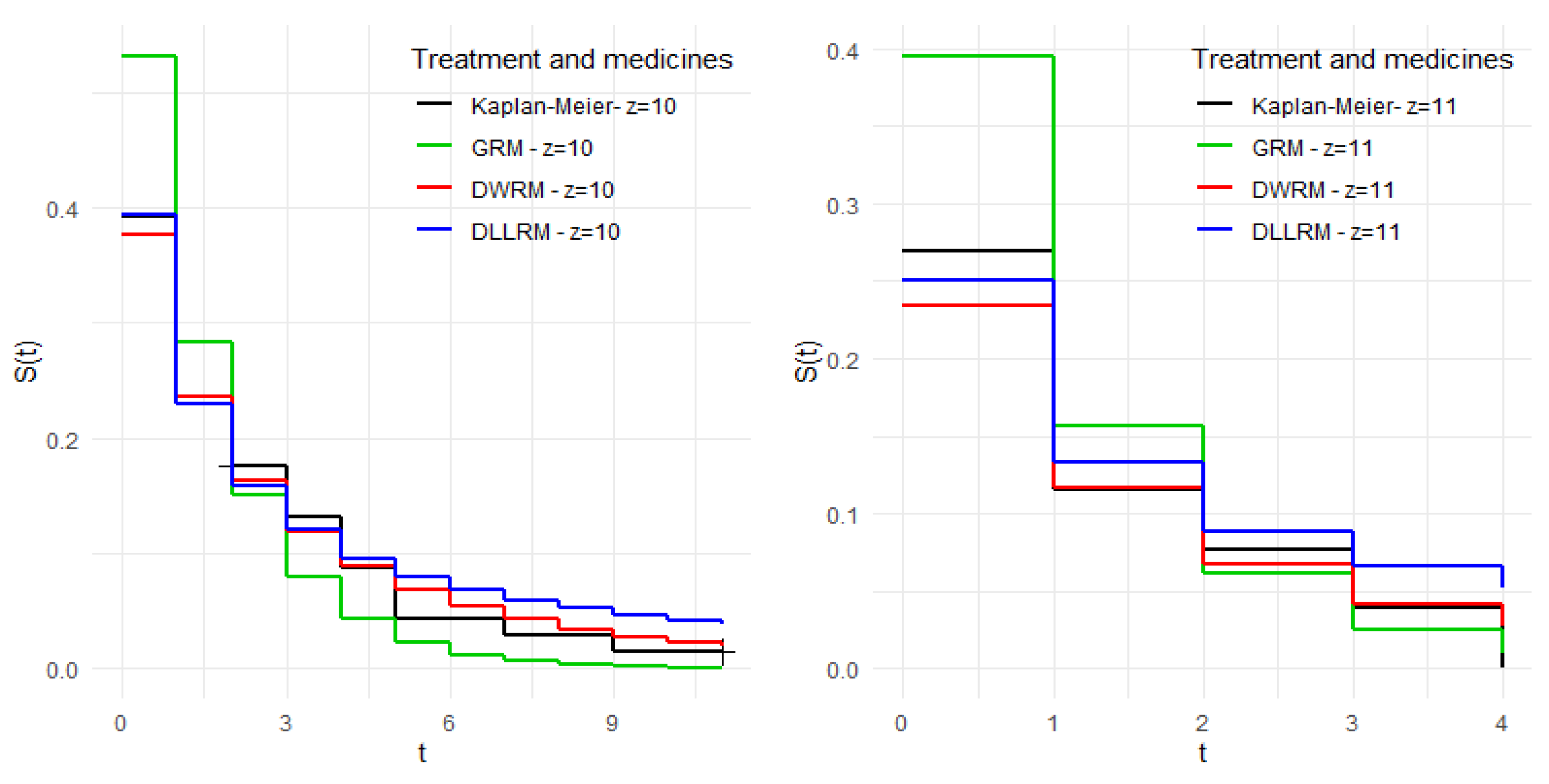
Note, through Figure 8, that for levels $z_1=1$; $z_2=0$ and $z_1=1$; $z_2=1$, the so-called traditional models behaved similarly to the model under study. However, for the other levels, the estimates of these models are more distant from the empirical estimates compared to the model under study, providing indications that the proportional odds hazard structure for discrete data provides a better fit to the data when compared to traditional discrete models.

6. Conclusions

The proportional odds hazard model (POHM) presented in this paper is a regression model developed for discrete data that has been used in the literature because it has the advantage of facilitating the interpretation of its coefficients without having to worry about using the baseline hazard. However, in certain studies, correctly informing the baseline hazard is essential.

In this study, the POHM was formulated considering the following distributions: discrete Weibull of [10], geometric and discrete log-logistic. The inferential process was developed in a survival analysis context using the maximum likelihood estimation method. The results obtained on simulated data showed evidence of the asymptotic properties of the estimators for two different baseline distributions. Furthermore, the model proposed by adopting three different baseline distributions (geometric, discrete Weibull and discrete log-logistic) showed a good fit to the real data set, demonstrating that the estimation method developed and the use of baseline distributions for discrete random variables used to develop the POHM is a highly viable alternative for modeling discrete survival data with covariates.