Article

Decomposition of Fuzzy Relations: An Application to the Definition, Construction and Analysis of Fuzzy Preferences

by
María Jesús Campión
1,†,
Esteban Induráin
2,*,† and
Armajac Raventós-Pujol
1,3,†
1
Inarbe (Institute for Advanced Research in Business and Economics) and Departamento de Estadística, Informática y Matemáticas, Universidad Pública de Navarra, 31006 Pamplona, Spain
2
InaMat2 (Institute for Advanced Materials and Mathematics) and Departamento de Estadística, Informática y Matemáticas, Universidad Pública de Navarra, 31006 Pamplona, Spain
3
Departamento de Análisis Económico: Economía Cuantitativa, Universidad Autónoma de Madrid, 28049 Madrid, Spain
*
Author to whom correspondence should be addressed.
These authors contributed equally to this work.
Axioms 2023, 12(12), 1077; https://doi.org/10.3390/axioms12121077
Submission received: 3 November 2023 / Revised: 21 November 2023 / Accepted: 22 November 2023 / Published: 24 November 2023

Abstract

:
In this article, we go deeper into the study of some types of decompositions defined by triangular norms and conorms. We work in the spirit of the classical Arrovian models in the fuzzy setting and their possible extensions. This allows us to achieve characterizations of existence and uniqueness for such decompositions. We provide rules to obtain them under some specific conditions. We conclude by applying the results achieved to the study of fuzzy preferences.

1. Introduction

1.1. Motivation of This Manuscript

Let us consider an individual that defines her/his preferences on a nonempty set X. To start with, let us assume that those preferences are crisp binary relations on X, so that given two elements x , y X and a binary relation R either x is related to y through R or it is not. In other words, understanding R as a subset of the Cartesian product X × X , we have that either ( x , y ) R or else ( x , y ) R . In that crisp setting, R is then a crisp subset of X × X ; that is, the characteristic function χ R that defines R can only take the values 0 or 1. Thus, χ R ( x , y ) = 1 means that x is related to y by means of R , whereas χ R ( x , y ) = 0 means that x is not related to y through R .
In the crisp approach, a preference on X is usually understood as a binary relation that is transitive and complete. (A complete binary relation is also known in the literature as a total binary relation. We also remark that a complete binary relation is also reflexive.) This is also known as a total preorder. We will use the notation ≿. In association with it, we may consider also two binary relations, namely ≻ and ∼, called, respectively, the strict preference and the indifference. x y if and only if it is not true that y x , and x y if and only if both x y and y x are true ( x , y X ) . With this definition, the total preorder ≿ decomposes as , and this decomposition is unique (see Section 2).
Unlike the crisp approach, in the fuzzy setting a fuzzy binary relation R on a nonempty set X is now understood as a fuzzy set of the Cartesian product X × X , so that now the indicator (also know as the membership function) of R is a map χ R : X × X [ 0 , 1 ] . It may take any possible value from 0 (no relationship at all, absolute negation) to 1 (total relationship, total evidence). Intermediate values give us, then, an idea of uncertainty.
To now start working in the fuzzy setting, some rather important facts should be pointed out:
1.
There are many nonequivalent extensions of the notions of completeness and/or transitivity, so that many possible definitions of the concept of a fuzzy total preorder could appear (see Section 2).
2.
Once a particular definition of a fuzzy total preorder, say R, has been chosen, we may try to decompose it by means of two fuzzy binary relations P and I, so that, in a way, the triplet ( R , P , I ) behaves as the decomposition ( , , ) of a crisp total preorder ≿. However, the definitions of what we mean by a fuzzy decomposition are neither unique nor equivalent (see Section 3).
3.
Again, even if we have chosen some particular definition of a fuzzy decomposition, it may happen that a given fuzzy preorder could still have more than one possible decomposition of that kind. In other words, now the decompositions are not necessarily unique (see Section 4 and Section 5).

1.2. A Revision of the Literature on Decompositions of Fuzzy Binary Relations

The problem of choosing definitions when generalizing crisp concepts is widespread in the fuzzy literature [1,2,3,4,5]. The study of preference structures is not an exception. For example, some authors study decompositions into two fuzzy binary relations P and I [5,6,7,8], whereas others study them in three relations: P, I and an additional one representing the idea of incomparability [9,10,11,12,13].
Our study on decompositions was first motivated by the need for a solid framework for fuzzy Arrovian models (see a complete survey in [3] (Chapter 4)). These models are a fuzzy extension of the well-known model introduced by Arrow in 1951, in the crisp setting, studying ranking aggregation [14]. In these fuzzy models, the decomposition of a preference plays an essential role, and it can be decisive in determining when it is possible to aggregate preferences. (We can illustrate the importance of decompositions comparing the models studied in [15] (Proposition 3.14) and [16] (Proposition 3.1). Their definition only differs in the chosen decomposition rule. In the former case, it is possible to aggregate preferences, but it is not possible in the second case.) In most of the literature, decompositions are defined using triangular norms and conorms (in the sequel, we will write t-norms (triangular norms) and t-conorms (triangular conorms) for short) (as generalizations of the crisp intersection and crisp union). Although in the earliest models decompositions were defined using a t-norm and a t-conorm playing the roles of the intersection and the union [15], in subsequent works the requirements for decompositions were weakened: the authors only used a single t-conorm in addition to a condition to assure that the fuzzy decomposition was a generalization of the dichotomic one with values in { 0 , 1 } [3,5,6,17]. One of our goals in our study is understanding the differences between both types of decomposition (strong and weak decompositions) and the reason behind this change.
The main difference in preference modeling in these Arrovian models and some of the works cited above [8,9,10,11,12,13] is the definition of asymmetry for the strict preference P as well as the nonexistence of an incomparability relation. The second one seems reasonable since the preferences are complete in Arrow’s original model. That is, two alternatives are always comparable. However, the choice of the asymmetry on fuzzy relations requires a deeper justification. Despite the fact that the most intuitive generalization requires T ( P ( x , y ) , P ( y , x ) ) = 0 for some t-norm T (see [8]), most of the researchers in this area have stood for strict preferences without both conjugated pairs with a positive degree (i.e., P ( x , y ) , P ( y , x ) > 0 ), and, as Dutta explained in one of the earliest articles [15], it is the most restrictive conception of asymmetry.
The reasons behind both choices make sense when we take into account the historical perspective. The introduction of fuzzy preferences in the Arrovian model was motivated by escaping from Arrow’s impossibility theorem [14]. As we have explained before, when fuzziness is introduced, many possible extensions of the concepts and definitions (unique in the original model) arise. These new definitions must make sense in the problems social scientists are studying. We look for models allowing preference aggregation rules, but in many cases, they need to remain as close as possible to a dichotomic interpretation. For instance, Duddy and Piggins studied aggregation rules where individual preferences were rankings and social preferences were fuzzy [18]. Billot also argues that any transitivity defined by t-norms will contradict the independence of irrelevant alternatives principle and they should be avoided (the independence of irrelevant alternatives is an (more philosophic than mathematical) assumption that states that if you take as input a set of alternatives and their characteristics, the input should not depend on extra-group characteristics) [1] (Section 1.1.2). In the same spirit, Dutta recognizes he chose the most restrictive form of asymmetry [15] because his study was looking for the minimum fuzzification needed to obtain aggregation rules. Moreover, his assumption has not been the object of remarkable criticism in subsequent studies (e.g., [3,5,6,16]).
For example, consider the case in which R ( x , y ) = 0.9 and R ( y , x ) = 0.05 . Here, x is clearly preferred over y, so under the assumption made by Dutta and others, it makes sense to state that P ( y , x ) = 0 . Moreover, compared with the situation R ( x , y ) = 1 and R ( y , x ) = 0 , it makes sense that P ( x , y ) > P ( x , y ) because of the differences in intensities between R and R . Then, we could argue that P must be a fuzzy relation satisfying the most restrictive asymmetry when an alternative is clearly preferred over the other. However, this argument does not lack criticism: consider the case in which R ( x , y ) = 0.65 and R ( y , x ) = 0.64 . Can we state that x is clearly preferred over y? In this case, saying that P ( x , y ) > 0 and P ( y , x ) = 0 lacks real meaning, and it should not be taken into account by practitioners. Nevertheless, cases such as the first example have prevailed over the second, and the restrictive notion of asymmetry is imposed. One of its reasons is, probably, that the Pareto condition loses its importance if other types of asymmetries are accepted. (The Pareto condition states that if all agents strictly prefer an alternative over another, the social preference must do it (see, e.g., [3]). The Pareto condition is the most accepted condition in the Arrovian model and is the backbone of the aggregation functions structure.)
It is worth mentioning that not all social scientists share the same opinion. Llamazares, in his study of decompositions [8], justifies his choice of asymmetry by quoting Blin [19] and Barret and Pattanai [20]: «[the vagueness] arises through the multiplicity of dimensions underlying preferences», and for that reason P ( x , y ) > 0 and P ( y , x ) > 0 can coexist. However, we have to mention that most of the works of Barret and Pattanaik in fuzzy preferences aggregation only work with strict preferences, and they do not have to deal with the decomposition problem nor the differences between weak and strict preferences [21,22].

1.3. Aim and Objectives

Our main objective is to generalize to the fuzzy context the classical decomposition of a preference or complete preorder, typical of the crisp case. Since uniqueness no longer occurs in fuzzy decompositions, we need to search for the decompositions that are closest or most similar to those used in the crisp setting, keeping in mind the Arrow models in classic Social Choice (crisp) and their possible generalizations to the fuzzy context.
It is also our intention to establish general definitions, inherent to this fuzzy Arrovian context. We wish the new ones that we will introduce to be considered “normative”, in the sense that they could encompass those that have already been introduced in the specialized literature on this matter.

1.4. Contents of This Manuscript

Having in mind the previous discussion, the scheme of this manuscript is as follows:
After the introduction, a section of preliminaries furnishes the basic definitions that will be used along the whole paper. We pay attention there to classical concepts in fuzzy set theory. Section 3 introduces then the key concept of a decomposition of a fuzzy binary relation. Among the main families of decompositions, we will consider the so-called strong and weak ones, respectively, analyzed in Section 4 and Section 5. In Section 6, we apply the results of the previous sections on the decomposition of preferences in the context of fuzzy Arrovian models. Finally, in Appendix A, we will give some geometrical ideas about the existence of decompositions when spaces of fuzzy binary relations are restricted by transitivity or completeness conditions. And we close this paper in Appendix B, applying our results to some of the most known t-norms and t-conorms.

2. Preliminaries

In this article, X will always denote a nonempty set.
Definition 1.
A binary relation R on X is a subset of the Cartesian product X × X . Given two elements x , y X , we will use the standard notation x R y to express that the pair ( x , y ) belongs to R .
In association with a binary relation R on X, we consider its negation (respectively, its transpose) as the binary relation R c (respectively, R t ) on X given by ( x , y ) R c ( x , y ) R for every x , y X (respectively, given by ( x , y ) R t ( y , x ) R , for every x , y X ) . We also define the adjoint R a of the given relation R , as R a = ( R t ) c .
A binary relation R defined on a set X is called the following terms:
(i) 
Reflexive if x R x holds for every x X ;
(ii) 
Irreflexive if ¬ ( x R x ) holds for every x X ;
(iii) 
Symmetric if R and R t coincide;
(iv) 
Antisymmetric if R R t { ( x , x ) : x X } ;
(v) 
Asymmetric if R R t = ;
(vi) 
Complete if R R t = X × X ;
(vii) 
Transitive if x R y y R z x R z for every x , y , z X .
In the particular case of a set X where some kind of ordering has been defined, the standard notation is different.
Definition 2.
A preorder ≿ on X is a binary relation on X that is reflexive and transitive. An antisymmetric preorder is said to be an order. A total preorder ≿ on a set X is a preorder such that if x , y X then ( x y ) ( y x ) holds. If ≿ is a preorder on X, then as usual we denote the associated asymmetric relation by ≻ and the associated equivalence relation by ∼ and these are defined by x y ( x y ) ¬ ( y x ) and x y ( x y ) ( y x ) .
A total preorder ≿ defined on X is usually called a (crisp) preference on X.
Definition 3.
Let R be a binary relation on X. We say that R decomposes into a symmetric binary relation (denoted by R s ) and an asymmetric binary relation (denoted by R a ) if R = R a R s and R a R s = .
Proposition 1.
Let ≿ be a preorder on a set X. It decomposes into ≻ and ∼. It is the unique decomposition of ≿ into asymmetric and symmetric relations.
Proof. 
See the proof in [23] (Theorem 1). ☐
Definition 4.
A fuzzy subset H of X is defined as a function μ H : X [ 0 , 1 ] . The function μ H is called the membership function of H. In the particular case when μ H is dichotomic and takes values in { 0 , 1 } , the corresponding subset defined by means of μ H is a subset of X in the classical crisp sense (the term crisp is usually understood in these contexts as meaning nonfuzzy).
Definition 5.
A fuzzy binary relation on X is a function R : X × X [ 0 , 1 ] . We say that R is symmetric if R ( x , y ) = R ( y , x ) for every x , y X , and we say that R is asymmetric if, for every x , y X , R ( x , y ) > 0 implies that R ( y , x ) = 0 holds. Moreover, R is said to be reflexive if R ( x , x ) = 1 for any x X .
Definition 6.
A triangular norm (t-norm for short) is a function T : [ 0 , 1 ] × [ 0 , 1 ] [ 0 , 1 ] satisfying the following properties:
(i) 
Boundary conditions: T ( x , 0 ) = T ( 0 , x ) = 0 , and T ( x , 1 ) = T ( 1 , x ) = x , for every x [ 0 , 1 ] .
(ii) 
Monotonicity: T is nondecreasing with respect to each variable; that is if x 1 x 2 and y 1 y 2 , then T ( x 1 , y 1 ) T ( x 2 , y 2 ) holds true.
(iii) 
T is commutative: T ( x , y ) = T ( y , x ) holds for every x , y [ 0 , 1 ] .
(iv) 
T is associative: T ( x , T ( y , z ) ) = T ( T ( x , y ) , z ) holds for any x , y , z [ 0 , 1 ] .
Definition 7.
A triangular conorm (t-conorm for short) is a function S : [ 0 , 1 ] × [ 0 , 1 ] [ 0 , 1 ] satisfying the following properties:
(i) 
Boundary conditions: S ( x , 0 ) = S ( 0 , x ) = x , and S ( x , 1 ) = S ( 1 , x ) = 1 , for every x [ 0 , 1 ] .
(ii) 
Monotonicity: S is nondecreasing with respect to each variable; that is, if x 1 x 2 and y 1 y 2 , then S ( x 1 , y 1 ) S ( x 2 , y 2 ) holds true.
(iii) 
S is commutative: S ( x , y ) = S ( y , x ) holds for every x , y [ 0 , 1 ] .
(iv) 
S is associative: S ( x , S ( y , z ) ) = S ( S ( x , y ) , z ) holds for any x , y , z [ 0 , 1 ] .
Henceforth, the symbol T will denote a t-norm whereas the symbol S will stand for a t-conorm.
Remark 1.
(i) 
In this article, we will use t-norms and t-conorms to define the decomposition of a fuzzy binary relation. However, in the proofs below, we will only use properties i and i i of Definitions 6 and 7. This fact shows that we could define a decomposition with respect to a more general category of operators (for example preaggregation functions [24], copulas [25], fusion functions [26], mixture functions [27], overlap functions [28], penalty functions [29], etc.).
(ii) 
We have decided to use t-norms and t-conorms because they are the fuzzy generalizations of the classic intersection and union operators and, more importantly, because we want to be coherent with the pre-existing literature that analyzes, studies and uses decompositions in practice [3,5,6].
(iii) 
In addition, in the search of an even more general setting than the one considered here with t-norms and t-conorms, we should also make a choice (e.g., copulas) and update to the current year the existing literature. However, as far as we know, the most recent literature on these more general categories of operators seems to use decompositions only in particular cases and regarding some very concrete and particular question or application in practice, mainly related to algorithms (see [30]) or computer science (see [31]).
(iv) 
Notice, in addition, that those new references do not work, a priori, with the intention of constructing a normative theory that could encompass other previously issued decompositions, as we intend to construct here for t-norms and t-conorms. Instead, as already said, they just work with quite particular and concrete aspects of practice (see, e.g., [30]).
(v) 
Other totally different kinds of decompositions of fuzzy relations, paying attention to algebraical aspects of matrix theory, may be seen in [32]. However, they seem to be unrelated to the scope of the present manuscript.
Let R 1 , R 2 and R 3 be fuzzy binary relations on X. Then, the notation R 1 = T ( R 2 , R 3 ) will mean from now on that, for every x , y X , R 1 ( x , y ) = T ( R 2 ( x , y ) , R 3 ( x , y ) ) holds. Obviously, we use a similar convention for a t-conorm S.
Definition 8.
Let T and S, respectively, be a t-norm and a t-conorm. An element a ( 0 , 1 ) is said to be a 0-divisor of T if there exists some b ( 0 , 1 ) such that T ( a , b ) = 0 . Also, an element a ( 0 , 1 ) is called a 1-divisor of S if there exists some b ( 0 , 1 ) such that S ( a , b ) = 1 .
Definition 9.
A t-norm T (respectively, a t-conorm S) is called strict if it is strictly increasing on each variable on ( 0 , 1 ] 2 (respectively, [ 0 , 1 ) 2 ). In other words, for all x , y , z [ 0 , 1 ] with x < y , T ( z , x ) < T ( z , y ) if 0 < z (respectively, S ( z , x ) < S ( z , y ) if z < 1 ).

3. Decompositions of Fuzzy Binary Relations

In the present manuscript, we study decompositions based on t-norms and t-conorms, respectively, playing the crisp intersection and union roles. This approach motivates the following definition used by Dutta [15] in his first article studying the fuzzy Arrovian model. Recently, it has been rescued by Subramanian [33] in his study of the Arrovian model.
Definition 10.
Let R , P and I be fuzzy binary relations on X (with P an asymmetric fuzzy binary relation and I a symmetric binary relation). Let T (respectively, S) stand for a triangular norm (respectively, conorm). We say that R strongly decomposes, with respect to ( T , S ) , into ( P , I ) , if R = S ( P , I ) and T ( P , I ) = 0 .
Even if the decomposition defined above is the natural generalization of the usual crisp decomposition, it is not widespread in the literature. Indeed, many authors use some weaker versions [3,5,6,15,16]. The following definition follows the same spirit but disregards the role that any t-norm could play:
Definition 11.
Let R be a fuzzy binary relation on a set X. Let S be a t-conorm. We say that R weakly decomposes into ( P , I ) (with P an asymmetric fuzzy binary relation and I a symmetric binary relation) if R = S ( P , I ) and if for every x , y X it holds true that if I ( x , y ) = 1 , then P ( x , y ) = 0 .
We have two comments about the definitions above. First, notice that the weak decomposition is more general than the stronger one. Moreover, they are not equivalent. The following example proves it:
Example 1.
Let X = { x , y } and let R be a fuzzy binary relation defined on X as follows: R ( x , y ) = R ( x , x ) = R ( y , y ) = 1 and R ( y , x ) = 0.5 . We define the symmetric relation I as I ( x , y ) = 0.5 and I ( x , x ) = I ( y , y ) = 1 . If we define P as P ( x , y ) = 1 and 0 on the remaining cases, we can check that R weakly decomposes into ( P , I ) with respect the t-conorm maximum S max . However, R does not strongly decomposes into ( P , I ) with respect to the conorm S max and any t-norm T because T ( 1 , 0.5 ) = 0.5 0 .
The second observation is about the second condition in Definition 11. It has been introduced after removing the t-norm from Definition 10 because we need decompositions to be generalizations of the crisp one (Definition 3). It implies that crisp relations must decompose into two crisp relations ( P , I ) and these must be unique. But, without this condition, if X = { x , y } and a fuzzy binary relation R on X is defined as R ( x , y ) = R ( y , x ) = R ( x , x ) = R ( y , y ) = 1 , it decomposes to ( P , I ) with I ( x , y ) = I ( x , x ) = I ( y , y ) = 1 and P ( x , y ) = 0.5 and 0 otherwise.
Finally, in a previous paper [23] the authors proved some necessary conditions for these kinds of decompositions. We will include them here for the sake of completeness.
Proposition 2.
Let S be a t-conorm. Let R be a fuzzy binary relation defined on X. Assume that R can be expressed as R = S ( P , I ) (where I (respectively, P) is a symmetric (respectively, asymmetric) fuzzy binary relation). Then, for every x , y X it holds that I ( x , y ) = min { R ( x , y ) , R ( y , x ) } .
Proof. 
See the proof in [23] (Proposition 2). ☐
Proposition 3.
Let S be a t-conorm. Every fuzzy relation R on X can be expressed as R = S ( P , I ) (where I (respectively, P) is a symmetric (respectively, asymmetric) fuzzy binary relation) if and only if S is continuous in the first coordinate (with respect to the Euclidean topology on the unit interval [ 0 , 1 ] ).
Proof. 
It is straightforward to notice that the proof is in everything similar to that of [23] (Proposition 3). That is why we omit it here. ☐
The proof of Proposition3 in [23] gave us a method to obtain a candidate for the asymmetric component P computed from R. In other words, if R decomposes, one of its decompositions is the pair ( P , I ) provided by this method.
As Proposition 2 states, the I component is a minimum, whereas the candidate for the P component is defined as P ( x , y ) = inf { t [ 0 , 1 ] : S ( t , I ( x , y ) ) R ( x , y ) } .
To abbreviate that, in the sequel we use the notation P ( x , y ) = I ( x , y ) S R ( x , y ) .
Remark 2.
Notice that since S is commutative, continuity on one of its coordinates implies continuity on both coordinates (considered separately). However, it does not imply the continuity for a general symmetric real function. However, since S is nondecreasing, both conditions are equivalent (see, e.g., [34] (Proposition 1)). Then, in Proposition 3, S being continuous in the first coordinate is equivalent to S being continuous.
In spite of this fact, in this article we will specify over which component S must be continuous. We proceed this way because the same results could be useful for the noncommutative operators we have listed in Remark 1.
In the literature, there are similar results to that stated in Proposition 2 (see [3,5,6]). In fact, even Fono and Andjiga [6] use a similar strategy to the one we use in Proposition 3. However, the definitions of decompositions used in these works are more general than the weak decomposition defined in the present manuscript. Their definition is so general that they have to impose additional constraints. They end up studying regular decompositions, and these are actually less general than Definition 11.
In addition, in contrast to the work of Fono and Andjiga [6], here we do not assume a priori any continuity condition on S. Although they assume upper continuity in the definition of its decomposition, we have seen using Proposition 3 above that the continuity on the first component is a necessary condition for the existence of our decompositions. So, the continuity condition over S is a consequence of S admitting decompositions, and it is not imposed a priori.
In Section 4, we will characterize the existence and the uniqueness of strong decompositions, whereas in Section 5 we characterize them for weak decompositions.
Given a fuzzy binary relation R, we could study the conditions that should satisfy R in order to decompose. However, in the Social Choice models [3,5,15,16] we usually impose that all of the binary relations of a suitable set must admit a decomposition. For that reason, we will start studying under which conditions all elements in BR X (the set of fuzzy binary relations on X) decompose. Next, in Appendix A we will explore the decomposition on subsets of BR X , mainly the subsets obtained by imposing some kind of transitivity and connectedness to fuzzy binary relations.

4. Analysis and Structure of Strong Decompositions of Fuzzy Binary Relations

This section contains two main results. We characterize the existence and the uniqueness of strong decompositions based upon the divisors of a t-norm T and a t-conorm S. First, we start with some more specific (and preparatory) results, which will motivate the general theorems to be proved next.
First, we focus on the case in which the used t-norm is the drastic t-norm T D (see its definition in Example A1 in Appendix B). The following results prove that being decomposable with respect T D is a necessary condition for being decomposable with respect to any other t-norm.
Proposition 4.
Let R be a fuzzy binary relation on X. Let S be a t-conorm and T a t-norm. If R strongly decomposes into ( P , I ) (with respect to S and T), then R decomposes into ( P , I ) with respect to S and T D .
Proof. 
It is straightforward if we use the following fact: every t-norm is bounded below by the drastic t-norm. ☐
Considering the result above, we characterize as a first step the existence of decompositions with respect T D .
Proposition 5.
Let S be a t-conorm continuous in the first component. Any R BR X is strongly decomposable with respect to S and T D if and only if every t ( 0 , 1 ) is a 1-divisor (with respect to S).
Proof. 
To prove the direct implication, let t ( 0 , 1 ) and consider a fuzzy binary relation R such that, for a pair of values x , y X , R ( x , y ) = 1 and R ( y , x ) = t . By hypothesis, there exist P and I such that 1 = R ( x , y ) = S ( P ( x , y ) , I ( x , y ) ) and P ( x , y ) 1 because T D ( P ( x , y ) , I ( x , y ) ) = 0 . Hence, t = I ( x , y ) is a 1-divisor.
To prove the converse implication, it is enough to see that the weak decomposition ( P , I ) proposed in the proof of Proposition 3 satisfies, for every x , y X , that T D ( P ( x , y ) , I ( x , y ) ) = 0 . If we assume that T D ( P ( x , y ) , I ( x , y ) ) 0 , then P ( x , y ) > 0 , I ( x , y ) > 0 , and I ( x , y ) = 1 or P ( x , y ) = 1 . If I ( x , y ) = 1 , then R ( x , y ) = 1 and P ( x , y ) = inf { t [ 0 , 1 ] : S ( t , 1 ) 1 } = 0 , but this contradicts the fact that P ( x , y ) > 0 . Moreover, if P ( x , y ) = 1 (and I ( x , y ) 1 ), we state that R ( x , y ) = S ( P ( x , y ) , I ( x , y ) ) = 1 and, since I ( x , y ) ( 0 , 1 ) , I ( x , y ) is a 1-divisor. So, there is an s 0 ( 0 , 1 ) with S ( s 0 , I ( x , y ) ) = 1 . However, by the definition of P, we have that 1 = P ( x , y ) = inf { s [ 0 , 1 ] : S ( s , I ( x , y ) 1 } s 0 < 1 , and this is a contradiction. ☐
The above proposition makes us think that the relation between the 0-divisors (respectively, 1-divisors) of a t-norm T (respectively, of a t-conorm S) is the keystone in the existence of strong decompositions.
The argument in the proof is based upon avoiding T D ( P , I ) being positive. Since I could achieve any value (see Proposition 2), any of these values must have a 0-divisor.
The next step is the generalization of Proposition 5 to any t-norm. For that reason, we state the following definition.
Definition 12.
Let S (respectively, T) be a triangular conorm (respectively, a t-norm). Given any w [ 0 , 1 ] , we define the 1-interval associated with w as D S 1 ( w ) = { t [ 0 , 1 ] : S ( t , w ) = 1 } . (It is straightforward to check that D S 1 ( w ) and D T 0 ( w ) are intervals because of the monotonicity of S and T. Moreover, 1 D S 1 ( w ) and 0 D T 0 ( w ) are always satisfied.) Similarly, the 0-interval associated with w is defined by D T 0 ( w ) = { t [ 0 , 1 ] : T ( t , w ) = 0 } .
Proposition 6.
Let S and T, respectively, be a t-conorm and a t-norm, and let X be a set. Every fuzzy binary relation on X is strongly decomposable with respect to S and T if and only if for all w [ 0 , 1 ] it holds true that D S 1 ( w ) D T 0 ( w ) , and the triangular conorm S is continuous on the first coordinate.
Proof. 
To prove the direct implication, for every w [ 0 , 1 ] consider a fuzzy binary relation R with R ( x , y ) = 1 and R ( y , x ) = w . By hypothesis, R strongly decomposes into a pair ( P , I ) . We have that 1 = R ( x , y ) = S ( P ( x , y ) , I ( x , y ) ) and 0 = T ( P ( x , y ) , I ( x , y ) ) , and now using that w = I ( x , y ) (Proposition 2), we obtain that P ( x , y ) D S 1 ( w ) D T 0 ( w ) .
To prove the converse implication, we only need to see that the decomposition ( P , I ) obtained in the proof of Proposition 3 satisfies T ( P ( x , y ) , I ( x , y ) ) = 0 for all x , y X . To do so, we can assume without loss of generality that I ( x , y ) , P ( x , y ) > 0 . First, when R ( x , y ) = 1 , we have that P ( x , y ) = inf { t [ 0 , 1 ] : S ( t , I ( x , y ) ) 1 } = inf D S 1 ( I ( x , y ) ) . In this situation, we claim that P ( x , y ) = min D S 1 ( I ( x , y ) ) because S is continuous on the first component. Moreover, since P ( x , y ) is the minimum of D S 1 ( I ( x , y ) ) , and D S 1 ( I ( x , y ) ) D T 0 ( I ( x , y ) ) , we conclude that P ( x , y ) D T 0 ( I ( x , y ) ) and we see that T ( P ( x , y ) , I ( x , y ) ) = 0 . In addition, when R ( x , y ) < 1 , we define R ¯ as the fuzzy binary relation that coincides with R everywhere except on the pair ( x , y ) , for which we define R ¯ ( x , y ) = 1 . R ¯ decomposes into ( P ¯ , I ) . It can be checked, using the definition, that P ( x , y ) P ¯ ( x , y ) . Finally, notice that we are now in the previous situation already analyzed, because R ¯ ( x , y ) = 1 , and 0 = T ( P ¯ ( x , y ) , I ( x , y ) ) T ( P ( x , y ) , I ( x , y ) ) . ☐
Taking into account the previous proof, the condition of uniqueness is quite natural. The set D S 1 ( I ( x , y ) ) D T 0 ( I ( x , y ) ) contains all the possible values for the asymmetric part P ( x , y ) . Hence, in order to achieve uniqueness, it is enough to request this set to have just a single element.
Proposition 7.
Every binary fuzzy relation on X is strongly decomposable with respect to S and T, in a unique way, if and only if the t-conorm S is continuous in the first component and for all w [ 0 , 1 ] it holds true that | D S 1 ( w ) D T 0 ( w ) | = 1 .
Proof. 
Suppose that there are w , s , t [ 0 , 1 ] with s < t and such that s , t D S 1 ( w ) D T 0 ( w ) . We fix now a pair x , y X and define a binary relation R B X as R ( y , x ) = w and R ( a , b ) = 1 if ( a , b ) ( y , x ) . Additionally, we define three binary relations I , P , P B X for every a , b X as follows: I ( a , b ) = min { R ( a , b ) , R ( b , a ) } , P ( a , b ) = P ( a , b ) = R ( a , b ) I ( a , b ) if ( a , b ) ( x , y ) , P ( x , y ) = s and P ( x , y ) = t . It remains to prove that R strongly decomposes in ( P , I ) as well as ( P , I ) , and therefore the decomposition is not unique.
Using the arguments in the proof of Proposition 6 we only need to check that R ( x , y ) = S ( P ( x , y ) , I ( x , y ) ) = S ( P ( x , y ) , I ( x , y ) ) and 0 = T ( P ( x , y ) , I ( x , y ) ) = T ( P ( x , y ) , I ( x , y ) ) . But these assertions are indeed true because 1 = S ( s , w ) = S ( t , w ) and 0 = T ( t , w ) = T ( t , w ) by hypothesis.
Suppose that R strongly decomposes into ( P , I ) and ( P , I ) . Proposition 2 guarantees that I = I , so there are x , y X such that P ( x , y ) P ( x , y ) . Now, we define s = P ( x , y ) , t = P ( x , y ) and w = I ( x , y ) . To conclude, by the definition of a strong decomposition we can guarantee now that s , t D S 1 ( w ) D T 0 ( w ) . ☐
The main problem that we face when dealing with strong decompositions is that the conditions for their existence and uniqueness are too restrictive. In Appendix B, we can see some examples for the most usual t-norms and t-conorms. For that reason, we will study now a weaker version of a decomposition defined by only using a t-conorm.
Furthermore, another reason to proceed in that way is that the main literature, as far as we know, uses this second type of decomposition, namely the so-called weak decomposition.

5. Weak Decompositions of Fuzzy Binary Relations

We can encounter, in the specialized literature, some pioneer introductions of decompositions similar to the weak ones considered here, as isolated proposals to derive two binary relations from a single one generalizing the crisp decompositions. However, no general framework discussing decompositions was proposed in those studies [1,4,15,16,35].
Richardson in [36] proposed a general framework, and it has been adopted by other authors, such as Fono and Andjiga in [6] or Gibilisco et al. in [3]. The general framework introduced by Richardson is a priori more general than Definition 11. However, in order to obtain results, they request that all their decompositions satisfy a property that they call simplicity, and then, because of having asked this extra property, our Definition 11 becomes more general than theirs with that condition of “simplicity” added.
Proposition 8.
Let S be a t-conorm and X a set. Every fuzzy relation R on X admits a weak decomposition if and only if S is continuous in the first coordinate (with respect to the Euclidean topology on the unit interval [ 0 , 1 ] ).
Proof. 
Notice that Proposition 3 guarantees the direct implication. For the converse implication, we also use the decomposition ( P , I ) defined from R proposed in the proof of Proposition 3. It only remains to show that such a pair is a weak decomposition. But this is indeed the case because, if I ( x , y ) = 1 (with x , y X ), then R ( x , y ) = 1 and P ( x , y ) = inf { t [ 0 , 1 ] : S ( t , I ( x , y ) ) R ( x , y ) } = 0 . ☐
In the following example, we compute some weak decompositions for the main t-conorms, using the formula from Proposition 3, namely P S = I S R .
Example 2.
Let R be a fuzzy binary relation on X. Let S be a t-conorm. Using the proof of Proposition 3, we can compute a decomposition ( P S , I ) of R with respect to several well-known t-conorms (Example A1 contains their definitions).
P max ( x , y ) = R ( x , y ) i f R ( x , y ) > R ( y , x ) , 0 o t h e r w i s e .
P S ( x , y ) = R ( x , y ) R ( y , x ) i f R ( x , y ) > R ( y , x ) , 0 o t h e r w i s e .
P S P ( x , y ) = R ( x , y ) R ( y , x ) 1 R ( y , x ) i f R ( x , y ) > R ( y , x ) , 0 o t h e r w i s e .
and I ( x , y ) = min { R ( x , y ) , R ( y , x ) } (for every x , y X ). We point out that these decompositions already appeared as suitable expressions in the previous literature, in this setting. For instance, P S max was considered in [15,35], P S in [4,15] and P S P in [3].
The last proposition in this section characterizes the uniqueness of weak decompositions (provided that they exist).
Proposition 9.
Let S be a t-conorm that is continuous in the first coordinate. Let R be a fuzzy binary relation on X. R has a unique weak decomposition in terms of S if and only if S is strictly increasing in the first coordinate. (Here, being strictly increasing has to be interpreted in the sense of Definition 9. No t-conorm is strictly increasing on the whole domain [ 0 , 1 ] 2 .)
Proof. 
Suppose that R decomposes into two distinct weak decompositions ( P , I ) and ( P , I ) . We can suppose without a loss of generality that there exist x , y X such that P ( x , y ) > P ( x , y ) . Also, I ( x , y ) 1 because P ( x , y ) > 0 . Hence, using the condition of strict increasingness, we see that R ( x , y ) = S ( P ( x , y ) , I ( x , y ) ) > S ( P ( x , y ) , I ( x , y ) ) = R ( x , y ) . Thus, we have obtained a contradiction, and, consequently, the decomposition is unique.
If S is not strict, there are s , t , w ( 0 , 1 ) with S ( s , w ) = S ( t , w ) and s t . We can define a binary relation R as R ( x , y ) = S ( s , w ) , R ( y , x ) = w for some x , y X and R ( a , b ) = 1 at any other pair ( a , b ) . It can be checked that R weakly decompose into ( P , I ) and ( P , I ) defined as I ( a , b ) = min { R ( a , b ) , R ( b , a ) } (for every a , b X ) and P ( x , y ) = s , whereas P ( x , y ) = t and P ( a , b ) = 0 at any other pair ( a , b ) . ☐
In the Appendix B, Table A1 furnishes information about decomposability, analyzing which ones among the main t-conorms can decompose all fuzzy binary relations.

6. Applications of Decompositions of Fuzzy Binary Relations into Preference Modeling under Uncertainty

In this section, we will apply the results of the previous sections about the decomposition of fuzzy binary relations to fuzzy Arrovian models.
In the literature, it is required to obtain a strict preference P and an indifference preference I from a weak preference R. However, the most common tendency is to first define a rule to obtain P and I and then study their properties [3,16,35]. Moreover, most of the authors in the Arrovian literature have used the type of decompositions studied in Section 4 and Section 5 to define such rules [3,5,6,15,37]. For instance, the probabilistic t-conorm induces a unique decomposition (see Equation (3) in Example 2 and Table A1). In the following pages, we will see that the decomposition generated by the probabilistic t-conorm satisfies the desired properties in fuzzy Social Choice. However, other conorms behave differently. Consider the following example:
Example 3.
Consider the following t-conorm S defined as the ordinal sum of a Łukasiewicz t-conorm (see [38] (Definition 3.68)).
S ( x , y ) = min { 0.5 , x + y } i f x , y 0.5 , max { x , y } o t h e r w i s e .
Any fuzzy binary relation weakly decomposes with respect to S because it is continuous (see Proposition 8). However, consider the binary relation R on X = { x , y } , defined as R ( x , y ) = R ( y , x ) = 0.5 and R ( x , x ) = R ( y , y ) = 1 . It decomposes into ( P , I ) , where I ( x , x ) = I ( y , y ) = 1 , P ( x , y ) = I ( x , y ) = 0.5 and P ( y , x ) = 0 . How could it be that, despite x and y playing the same role in R, x is strictly preferred over y? This is one of the situations that are avoided implicitly in fuzzy Arrovian models [3].
Therefore, we will first define what we expect (as Social Choice practitioners) from R, P, I and the relationship among them and, straightaway, how strong and weak decompositions can be used to obtain suitable decomposition rules.
With that purpose in mind, we use the concept of the preference structure (see, e.g., [39,40]) because its definition does not rely upon any concept related to decomposition rules. A preference structure is a triplet ( R , P , I ) of fuzzy binary relations satisfying the properties of Definition 13 below.
Definition 13
([41] (Definition 2.15)). Given a set X, a fuzzy preference on X is a triplet ( R , P , I ) of fuzzy binary relations on X that satisfies the following conditions:
(FP1) 
P ( x , y ) > 0 implies P ( y , x ) = 0 , for all x , y X (P is asymmetric);
(FP2) 
I ( x , y ) = I ( y , x ) , for all x , y X (I is symmetric);
(FP3) 
P ( x , y ) R ( x , y ) for every x , y X ;
(FP4) 
R ( x , y ) > R ( y , x ) if and only if P ( x , y ) > 0 , for every x , y X ;
(FP5) 
If P ( x , y ) = 0 , then R ( x , y ) = I ( x , y ) , for all x , y X ;
(FP6) 
If I ( x , y ) I ( z , w ) and P ( x , y ) P ( z , w ) , then R ( x , y ) R ( z , w ) holds true for every x , y , z , w X .
We call R the weak preference component, P the strict preference component and I the indifference component.
Using this definition, we state a framework to study the decomposition rules. It is equivalent to the standard definitions in several fuzzy Arrovian models [3,6,15]. Now, we can use this framework to apply the decompositions studied in the previous sections to decomposition rules. First, we need to define what we understand as a decomposition rule:
Definition 14.
Let B be a family of fuzzy binary relations on a set X. A decomposition rule on B is a map ϕ : B BR X × BR X , such that for every R B , if ϕ ( R ) = ( P R , I R ) , then Λ R = ( R , P R , I R ) is a fuzzy preference in the sense of Definition 13.
Our goal in this section will be to study when the decompositions already introduced through Section 4 and Section 5 induce or are compatible with a decomposition rule, in the following sense of the next Definition 15.
Definition 15.
Let T be a t-norm, S a t-conorm and ϕ a decomposition rule on B BR X :
(i) 
We say that ϕ is ( T , S ) -strong (resp. S-weak) compatible if, for every R B , it holds true that ϕ ( R ) is a strong (resp. weak) decomposition of R with respect to T and S (resp. S).
(ii) 
We say that ϕ is induced by ( T , S ) (resp S) if ϕ is ( T , S ) -strong (resp. S-weak) compatible and for every R B it holds, in addition, that ϕ ( R ) is the unique decomposition of R, which induces a preference. That is, if ( P , I ) is a decomposition of R and ( R , P , I ) is a preference, then ϕ ( R ) = ( P , I ) . In that case, we denote by ϕ T , S (resp. ϕ S ) the induced decomposition rule.
Example 4.
The decomposition rule ϕ 1 ( R ) = ( P R 1 , I R ) defined in B = BR X as I R ( x , y ) = min { R ( x , y ) , R ( y , x ) } and P R 1 ( x , y ) = min { 0 , 1 2 ( R ( x , y ) R ( y , x ) ) } is neither ( T , S ) -strong nor S-weak compatible for any T and S: if R ( x , y ) = 1 and R ( y , x ) = 0 , then R ( x , y ) S ( P R 1 ( x , y ) , I R ( x , y ) ) .
Moreover, consider the decomposition rules ϕ 2 = ( P S , I R ) (see Example 2) and ϕ 3 = ( P S , I R ) defined as P S R ( x , y ) = 1 if 1 = R ( x , y ) > R ( y , x ) and P S ( x , y ) = P S ( x , y ) otherwise. They are both S -weak compatible, so neither of them are induced by S . Finally, Proposition 11 proves that ϕ S max is induced by S max .
First, we will focus on the case ( i ) in the Definition 15 above. We will study which t-norms and t-conorms admit decomposition rules compatible with them. Next, we will focus on the t-norms and t-conorms that induce decomposition rules (case ( i i ) ).
As in the previous sections, we will restrict our study to the case B = BR X , since other domains could lead to different results.
Proposition 10.
Let R be a fuzzy binary relation on X. Let S be a t-conorm and let T be a t-norm. If ( P , I ) is a strong or a weak decomposition of R with respect to T and S or respect to S, then the properties F P 1 , F P 2 , F P 3 , F P 5 and F P 6 and the direct implication in the statement F P 4 of Definition 13 hold true.
Moreover, the converse of F P 4 is satisfied if for every t [ 0 , 1 ) there exists a neighborhood of 0 in which S ( · , t ) is strictly increasing.
Proof. 
Conditions F P 1 and F P 2 are obtained from the definition of a decomposition. To prove F P 3 , notice that R ( x , y ) = S ( P ( x , y ) , I ( x , y ) ) S ( P ( x , y ) , 0 ) = P ( x , y ) .
To prove F P 5 notice that if P ( x , y ) = 0 , then R ( x , y ) = S ( P ( x , y ) , I ( x , y ) ) = S ( 0 , I ( x , y ) ) = I ( x , y ) .
Property F P 6 is a direct consequence of the monotonicity of S.
Finally, to prove the direct implication of F P 4 , observe that if R ( x , y ) > R ( y , x ) , by property F P 6 it follows now that [ I ( x , y ) > I ( y , x ) ] [ P ( x , y ) > P ( y , x ) ] holds true. But, since I is symmetric, so that I ( x , y ) = I ( y , x ) , we obtain P ( x , y ) > P ( y , x ) 0 .
Additionally, suppose that S satisfies the last property. If P ( x , y ) > 0 , then P ( y , x ) = 0 . Hence, we may now conclude that R ( y , x ) = S ( 0 , I ( y , x ) ) < S ( P ( x , y ) , I ( x , y ) ) = R ( x , y ) . ☐
In the following example, we can see a decomposition that satisfies all the properties above but with the converse implication in F P 4 and, consequently, does not give rise to a fuzzy preference.
Example 5.
Let R be a fuzzy binary relation defined on a set X. Consider the fuzzy binary relations P and I on X defined as follows:
P ( x , y ) = R ( x , y ) i f R ( x , y ) > R ( y , x ) , R ( x , y ) i f 1 > R ( x , y ) = R ( y , x ) , 0 o t h e r w i s e .
and I ( x , y ) = min { R ( x , y ) , R ( y , x ) } . Notice that R weakly decomposes into ( P , I ) with respect to S max and this decomposition is not the same as the one arising in Example 2.
The case of a weak decomposition with respect to S max is paradigmatic in the literature, and we will use it to motivate the main result in this section.
The decomposition (1) shown in Example 2 actually appeared early in the specialized literature [35], usually as a suitable decomposition rule in several contexts. The example above shows that it is not the unique weak decomposition with respect to S max . However, the following proposition proves that it is the unique decomposition that defines a fuzzy preference. That is, S max induces a decomposition rule.
Proposition 11.
Let R be a fuzzy binary relation on a set X. There exists a unique decomposition ( P , I ) of R with respect to the t-conorm S max satisfying that ( R , P , I ) is a fuzzy preference.
Proof. 
Consider a fuzzy binary relation R. The maximum is a continuous t-conorm. By Proposition 3, R is decomposable. Suppose that there are two different decompositions ( P , I ) and ( P , I ) of R such that both ( R , P , I ) and ( R , P , I ) are fuzzy preferences. First, by Proposition 2, I = I holds. If P P , we can assume, without a loss of generality, that there are x , y X with P ( x , y ) > P ( x , y ) .
From the equality R ( x , y ) = max { P ( x , y ) , I ( x , y ) } = max { P ( x , y ) , I ( x , y ) } , we obtain that R ( x , y ) = I ( x , y ) . Using that I ( x , y ) = min { R ( x , y ) , R ( y , x ) } (Proposition 2), we conclude that R ( x , y ) R ( y , x ) . We have finally arrived at a contradiction because, using F P 4 , we obtain that P ( x , y ) = 0 . ☐
Remark 3.
In Proposition 10, we have proved that the property of S “for every t, having a neighbourhood of 0 such that S ( t , · ) is strictly increasing” implies F P 4 .
If we could find a property of S equivalent to F P 4 , then the characterization of decompositions that are a preference would be completed. Unfortunately, Example 5 makes us think that such a property does not exist.
Assuming the existence of such a property q, S max may or may not satisfy q. If S max satisfied it, then all weak decompositions (with respect to S max ) should define a preference, but the decomposition in Example 5 does not define a preference. Conversely, if case S max satisfied q, then no weak decomposition should define a preference, but, according to Proposition 11, this is not true.
Then, such a property q should not exist. We conclude that an equivalence to F P 4 relies on something more than some properties of t-conorms.
The following proposition generalizes the previous example to any t-conorm that may be used in weak decompositions.
Proposition 12.
Let S be a t-conorm continuous in the first coordinate. S induces a weak decomposition rule if, and only if, for every w , t , s [ 0 , 1 ] with t s it holds true that, if S ( t , w ) = S ( s , w ) , then S ( t , w ) = w .
Proof. 
To prove the direct implication, suppose that there are w , s , t [ 0 , 1 ] such that S ( t , w ) = S ( s , w ) > w , and we will prove that there is an R BR X , which has at least two decompositions that induce fuzzy preferences.
To see that, given a pair a , b X , define a fuzzy binary relation R satisfying R ( a , b ) = S ( t , w ) ; R ( b , a ) = w and R ( c , d ) = 1 if ( c , d ) ( a , b ) and also ( c , d ) ( b , a ) . Consider now the three fuzzy binary relations I ( x , y ) = min { R ( x , y ) , R ( y , x ) } for all x , y X , P ( x , y ) = P ( x , y ) = 0 if ( x , y ) ( a , b ) , P ( a , b ) = t and P ( a , b ) = s .
Now, we can assert that ( P , I ) and ( P , I ) are weak decompositions of R. Moreover, ( R , P , I ) and ( R , P , I ) are preferences because they are defined by means of a decomposition and it is immediate to check that they indeed satisfy F P 4 . Therefore, S can not induce any decomposition rule.
Concerning the converse implication, we may notice that the unique property of the maximum used in the proof of Proposition 11 is just our hypothesis here. We could transcript the same proof after interchanging “From the equality R ( x , y ) = max { P ( x , y ) , I ( x , y ) } = max { P ( x , y ) , I ( x , y ) } we obtain that R ( x , y ) = I ( x , y ) with “From the equality R ( x , y ) = S ( P ( x , y ) , I ( x , y ) ) = S ( P ( x , y ) , I ( x , y ) ) we obtain that R ( x , y ) = I ( x , y ) ”. ☐
Remark 4.
Notice that if S is strictly increasing in the first coordinate, S satisfies the hypothesis of the Proposition 12, because if S ( t , w ) = S ( s , w ) , then w = 1 . This fact is consistent with the combination of Propositions 9 and 10, which also guarantees the existence of the induced decomposition rule ϕ S .

7. Conclusions

We are faced with variable forms of uncertainty and indeterminacy in many areas of life, which require reliable and effective treatment from the point of view of practice. All of this raises active control technical problems, within which the use of fuzzy controllers is now a natural possibility. Having in mind possible future research in order to cope with these problems, first of all it is necessary to state a solid theoretical background. In the present paper, we have intended to do so, around the notion of a fuzzy preference. This concept, defined as a triplet that reminds us of the usual weak preference, strict preference and indifference arising in the crisp setting, has been analyzed from the point of view of the existence of decompositions in which the fuzzy weak preference generates, in a way, the associated strict fuzzy preference as well as the fuzzy indifference. In the crisp setting, the decompositions are always unique, whereas this is no longer true in the fuzzy setting. Consequently, we have also analyzed questions related to the existence and uniqueness of decompositions of fuzzy preferences, as shown in the main sections of the present manuscript: Propositions 6–9 provide a novel characterization of the existence and uniqueness of strong and weak decompositions, whereas Proposition 12 characterizes the uniqueness of (weak) decomposition rules.
As already commented in Remark 1, in the present paper we have only used t-norms and t-conorms to define the decomposition of a fuzzy binary relation. However, in the proofs of some results achieved then, we did not use all of their properties. Therefore, thinking of future lines for research, we could also consider, and consequently define, a decomposition with respect to a more general category of operators. As we explained, the decision of using here only t-norms and t-conorms is due to the fact that they are the fuzzy generalizations of the classic intersection and union operators and, more importantly, because we wanted to be coherent with the pre-existing literature that analyzes, studies and uses decompositions in practice, paying special attention to the setting of Arrovian-like models in fuzzy Social Choice. Needless to say, in forthcoming works we could address the study of decompositions based upon other disparate operators.
We have been looking for a normative theoretical definition of a decomposition (at least for the case of t-norms and t-conorms). In this sense, we have compared our approach and the definitions we have launched with other ones encountered in the literature, showing that ours are more general. In our opinion, this is a relevant achievement at this stage: namely, with the definitions of a fuzzy decomposition that we have introduced, we provide the researcher with a generalized theoretical framework that systematically includes, as we have been discussing throughout the work, the (somewhat more restrictive) definitions that had already been introduced in this literature. At least, this applies, in our opinion, to decompositions associated with Arrovian-like models in the fuzzy setting.
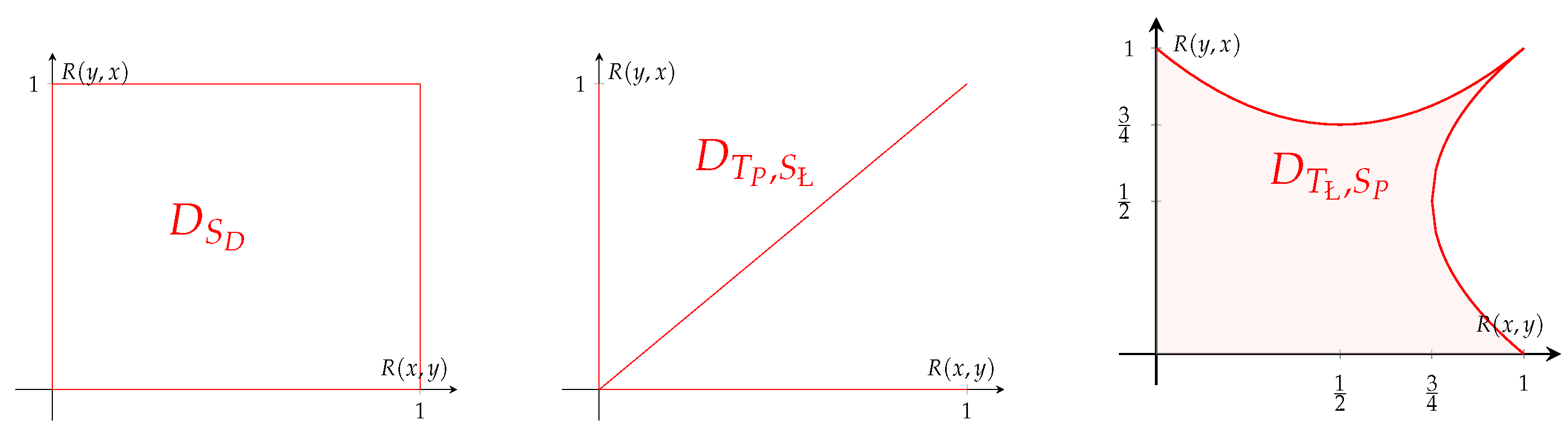
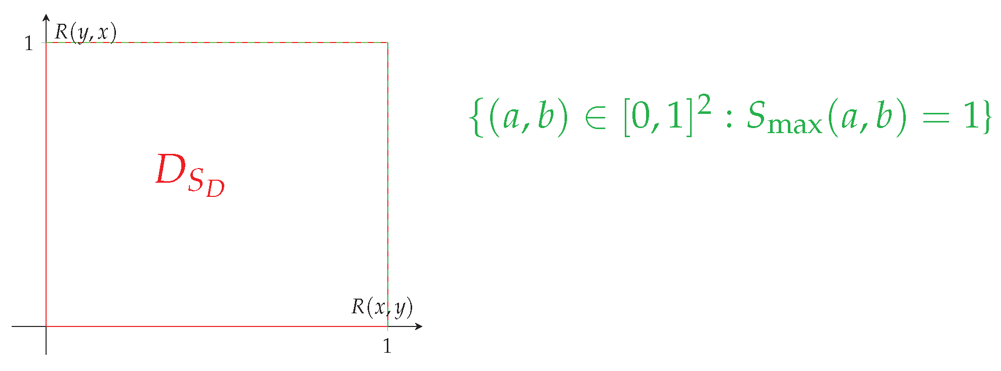
Last but not least, in the introduction of the present article, we have exposed that, in Social Choice, the sets of suitable preferences used to be restricted by transitivity and connectedness properties. In future work, we plan to extend our study to the sets of preferences restricted by these properties instead of BR X . The appendices contain a preliminary analysis of these sets where we expose a possible resolution of the problem by means of some figures. Based on our exploration, we hypothesize that when some connectedness condition is imposed, the possibility of the existence of decomposition rules increases.

Author Contributions

All authors have equally contributed. All authors have read and agreed to the published version of the manuscript.

Funding

This work has been partially supported by the research projects whose references are PID2019-108392GB-I00 (AEI/10.13039/501100011033), PID2021-127799NB-I00 and PID2022-1366274NB-I00 from the Ministry of Science and Innovation of Spain, as well as the Ayudas para la Recualificación del Sistema Universitario Español para 2021–2023, UPNA. Modalidad Margarita Salas funded by the European Union—NextGenerationEU and a predoctoral grant from the UPNA Research Institutes.

Data Availability Statement

No new data were created or analyzed in this study. Data sharing is not applicable to this article.

Acknowledgments

Thanks are given to the editor and three anonymous referees for their valuable suggestions and comments on a previous version of this manuscript.

Conflicts of Interest

The authors declare no conflict of interest.

Appendix A. Decompositions in Restricted Domains

As we have discussed in the Introduction, in most problems related to preferences, we require R to satisfy additional properties. Usually, they are some kind of transitivity and connectedness.
So, instead of studying the existence of decompositions on BR X , we could study them on the subsets defined by those transitivities and connectedness assumptions. In this section, we will give some geometric ideas about the conditions of existence for the decomposition in such domains, but we will not furnish any formal proof.
Consider BR X T (resp. BR X S ) the set of all T -transitive (resp. S -connected) binary relations of BR X . (A fuzzy binary relation R is said T -transitive if for every x , y , z X the inequality R ( x , z ) T ( R ( x , y ) , R ( y , z ) is satified. Moreover, it is said S -connected if for every x , y X S ( R ( x , y ) , R ( y , x ) ) = 1 . See [3] (Chapter 3) or [23] for a more extended exposition.) Notice that, a priori, the t-norm and the t-conorm defining the transitivity and the connectedness and the ones defining the decomposition may or may not coincide. For that reason, we use T and S to denote the ones corresponding to the transitivity and the connectedness and T and S for the ones defining the decomposition.
First, if ϕ is a decomposition rule on BR X , then its restriction to one of these sets will also be a decomposition rule.
However, could it be the case that, for example, there is no decomposition rule ϕ ( T , S ) -strong compatible on BR X but there are such rules on BR X T or on BR X S ? (We can make analogous suggestions about S-compatibility and decomposition rules induced by ( T , S ) or S.)
Before we go further on the possible answer to these questions, we need to introduce some terminology. First, as we have noticed before, the existence of decompositions and their uniqueness of a binary relation R depend only on the comparison between the values of R ( x , y ) and R ( y , x ) for every x , y X . We can illustrate this idea using the sets D S and D T , S defined below (see some examples in Figure A1):
D S = { ( a , b ) [ 0 , 1 ] 2 : a b x [ 0 , 1 ] a = S ( x , b ) a n d b = 1 x = 0 a n d b a x [ 0 , 1 ] b = S ( x , a ) a n d a = 1 x = 0 }
D T , S = { ( a , b ) [ 0 , 1 ] 2 : a b x [ 0 , 1 ] ;   a = S ( x , b ) a n d 0 = T ( x , b ) a n d b a x [ 0 , 1 ] ;   b = S ( x , a ) a n d 0 = T ( x , a ) }
The points a , b [ 0 , 1 ] 2 are the combinations of the values for R ( x , y ) and R ( y , x ) in which a decomposition is possible. So, we can state that a binary relation R is strongly decomposable with respect to T and S (resp. weakly decomposable with respect to S) if and only if, for every x , y X ( R ( x , y ) , R ( y , x ) ) D T , S (resp. D S ). Moreover, since BR X imposes no restrictions over the values, we can conclude that all binary relations are strongly (resp. weakly) decomposable if D T , S = [ 0 , 1 ] 2 (resp. if D S = [ 0 , 1 ] 2 ).
Now, we can state that in BR X T and apply the same results we have obtained for BR X . First, T -transitivity does not impose restrictions on the possible relations between R ( x , y ) and R ( y , x ) . In other words, given ( a , b ) [ 0 , 1 ] 2 , there is a T -transitive binary relation R with R ( x , y ) = a and R ( y , x ) = b . So, we can conclude that all binary relations in BR X decompose if, and only if, all binary relations in BR X T decompose.
Figure A1. Representations of D S D , D T P , S and D T , S P . Since none of these sets is the unit square [ 0 , 1 ] 2 , these combinations of t-norms and t-conorms do not allow decompositions (compare with Table A1).
Axioms 12 01077 g0a1
However, the restrictions imposed by connectedness are different. In this case, S -completeness imposes that S ( R ( x , y ) , R ( y , x ) ) = 1 . Since now some combinations of values will not be feasible, we conclude that all binary relations on BR X S will decompose if, and only if, { ( a , b ) [ 0 , 1 ] 2 : S ( a , b ) = 1 } D S (resp. if, and only if, { ( a , b ) [ 0 , 1 ] 2 : S ( a , b ) = 1 } D T , S ). We can see an example in Figure A2.
Figure A2. All binary relations in BR X S max weakly decompose with respect to S D because { ( a , b ) [ 0 , 1 ] 2 : S max ( a , b ) = 1 } D S D . However, not every binary relation in BR X weakly decomposes with respect to S D .
Axioms 12 01077 g0a2

Appendix B. Some Examples Using the Main t-Norms and t-Conorms

In this section, we have included the definitions of the most used t-norms and t-conorms [38]. We have also included in some tables which combinations allow decompositions and which ones are compatible and induce decomposition rules.
Example A1.
Here, we give a brief account of the most widespread t-norms and their respective dual t-conorms:
  • The minimum T min and the maximum S max are as follows:
    T min ( x , y ) = min { x , y } , S max ( x , y ) = max { x , y } .
  • The product T P and the probabilistic sum S P are as follows:
    T P ( x , y ) = x y , S P ( x , y ) = x + y x y .
  • The Łukasiewicz t-norm T and the Łukasiewicz t-conorm S are as follows:
    T ( x , y ) = max { 0 , x + y 1 } , S ( x , y ) = min { 1 , x + y } .
  • The drastic product T D and drastic sum S D are as follows:
    T D ( x , y ) = x i f y = 1 , y i f x = 1 , 0 o t h e r w i s e . S D ( x , y ) = x i f y = 0 , y i f x = 0 , 1 o t h e r w i s e .
And the associated divisor intervals are as follows:
D S D 1 ( w ) = { 1 } i f w = 0 , ( 0 , 1 ] i f w { 0 , 1 } , i f w = 1 . D T D 0 ( w ) = { 0 } i f w = 1 , i f w { 0 , 1 } , i f w = 0 .
D max 1 ( w ) = D S P 1 ( w ) = { 1 } i f w 1 , i f w = 1 . D min 0 ( w ) = D T P 0 ( w ) = { 0 } i f w 0 , i f w = 0 .
D S 1 ( w ) = [ 1 w , 1 ] , D T 0 ( w ) = [ 0 , 1 w ] .
Example A2.
The family ( T λ S S ) λ [ , ] of Schweizer–Sklar t-norms is defined as follows:
T λ S S ( x , y ) = min { x , y } i f λ = , T P ( x , y ) i f λ = 0 , T D ( x , y ) i f λ = , ( max { x λ + y λ 1 , 0 } ) 1 λ o t h e r w i s e .
And the respective family ( S λ S S ) λ [ , ] of t-conorms is defined as follows:
S λ S S ( x , y ) = max { x , y } i f λ = , S P ( x , y ) i f λ = 0 , S D ( x , y ) i f λ = , 1 max { ( 1 x ) λ + ( 1 y ) λ 1 , 0 } 1 λ o t h e r w i s e .
For λ , 0 , we have that
D T λ S S 0 ( w ) = { 0 } i f λ < 0 a n d w 0 , i f λ < 0 a n d w = 0 , λ ) 1 λ ] o t h e r w i s e .
D S λ S S 1 ( w ) = { 1 } i f λ < 0 a n d w 1 , i f λ < 0 a n d w = 1 , λ ) 1 λ , 1 ] o t h e r w i s e .
Example A3.
The family ( T λ H ) λ [ 0 , ] of Hamacher t-norms is defined as follows:
T λ H ( x , y ) = T D ( x , y ) i f λ = , 0 i f λ = x = y = 0 , x y λ + ( 1 λ ) ( x + y x y ) o t h e r w i s e .
And the respective family ( S λ H ) λ [ 0 , ] of t-conorms is defined as follows:
S λ H ( x , y ) = S D ( x , y ) i f λ = , 1 i f λ = x = y = 0 , x + y x y ( 1 λ ) x y 1 ( 1 λ ) x y o t h e r w i s e .
If λ , we have that D T λ H 0 ( w ) = D min 0 ( w ) and D S λ H 1 ( w ) = D max 1 ( w ) .
We have depicted the existence and uniqueness of strong and weak decompositions in BR X for these t-norms and t-conorms in Table A1. For that purpose, we have applied Propositions 6–9.
In Table A2, we have applied Propositions 10–12 to the same t-norms and t-conorms, obtaining the corresponding results for decomposition rules.
Table A1. Decompositions for main t-norms and t-conorms. The symbol means that the corresponding decomposition does not exist. ∃ means that it exists, but it is not unique, and ! means that a unique decomposition exists. Moreover, the characterization of the existence and the uniqueness of the strong decomposition of Schweizer–Skalar t-norms and t-conorms corresponds to the combination ( T λ S S , S λ S S ) with the same parameter λ .
SDrasticMaximumŁukasiewiczProbabilisticSchweizer–SklarHamacher
T
Drastic λ 0
0 < λ < +
λ = +
Minimum
ukasievicz ! λ 0
0 < λ < 1
λ = 1 !
λ > 1
Product
Schweizer–Sklar λ < 1
λ = 1 !
λ > 1
λ < 1
λ = 1 !
λ > 1
λ = +
Hamacher
Weak
decomposition
! λ =
< λ 0 !
0 < λ < +
λ = +
λ < + !
λ = +
Table A2. A representation of the relation between decomposition rules and decompositions. The symbol means that there is no decomposition rule compatible with such a decomposition. ∃CR means that there is a compatible decomposition rule with such decompositions. I D R means that the decomposition induces a decomposition rule. Finally, ? means that the results in this article do not shed some light on the case.
SDrasticMaximumŁukasiewiczProbabilisticSchweizer–SklarHamacher
T
Drastic C R λ 0
0 < λ < + ?
λ = +
Minimum
ukasievicz I D R λ 0
0 < λ < 1 ?
λ = 1 ?
λ > 1 ?
Product
Schweizer–Sklar λ < 1
λ = 1 I R D
λ > 1 C R
λ < 1
λ = 1 ?
λ > 1 ?
λ = +
Hamacher
Weak
decomposition
I D R C R I D R λ = I D R
< λ 0
0 < λ < + ?
λ = +
λ < + I R D
λ = +

References

  1. Billot, A. Economic Theory of Fuzzy Equilibria: An Axiomatic Analysis, 2nd ed.; Springer: Berlin/Heidelberg, Germany, 1995. [Google Scholar] [CrossRef]
  2. De Baets, B.; de Walle, B.; Kerre, E. Fuzzy preference structures without incomparability. Fuzzy Sets Syst. 1995, 76, 333–348. [Google Scholar] [CrossRef]
  3. Gibilisco, M.B.; Gowen, A.M.; Albert, K.E.; Mordeson, J.N.; Wierman, M.J.; Clark, T.D. Fuzzy Social Choice Theory; Springer International Publishing: Cham, Switzerland, 2014. [Google Scholar] [CrossRef]
  4. Montero, J.; Tejada, J. Some problems on the definition of fuzzy preference relations. Fuzzy Sets Syst. 1986, 20, 45–53. [Google Scholar] [CrossRef]
  5. Richardson, G. The structure of fuzzy preferences: Social choice implications. Soc. Choice Welf. 1998, 15, 359–369. [Google Scholar] [CrossRef]
  6. Fono, L.A.; Andjiga, N.G. Fuzzy strict preference and social choice. Fuzzy Sets Syst. 2005, 155, 372–389. [Google Scholar] [CrossRef]
  7. Fotso, S.; Fono, L.A. Arrow-type results under fuzzy preferences based on filter and ultrafilter. Fuzzy Sets Syst. 2015, 266, 101–113. [Google Scholar] [CrossRef]
  8. Llamazares, B. Factorization of fuzzy preferences. Soc. Choice Welf. 2005, 24, 475–496. [Google Scholar] [CrossRef]
  9. Díaz, S.; De Baets, B.; Montes, S. On the compositional characterization of complete fuzzy pre-orders. Fuzzy Sets Syst. 2008, 159, 2221–2239. [Google Scholar] [CrossRef]
  10. Díaz, S.; De Baets, B.; Montes, S. General results on the decomposition of transitive fuzzy relations. Fuzzy Optim. Decis. Mak. 2010, 9, 1–29. [Google Scholar] [CrossRef]
  11. Fodor, J.C. An axiomatic approach to fuzzy preference modelling. Fuzzy Sets Syst. 1992, 52, 47–52. [Google Scholar] [CrossRef]
  12. Llamazares, B. Characterization of fuzzy preference structures through Łukasiewicz triplets. Fuzzy Sets Syst. 2003, 136, 217–235. [Google Scholar] [CrossRef]
  13. Ovchinnikov, S.V.; Roubens, M. On fuzzy strict preference, indifference, and incomparability relations. Fuzzy Sets Syst. 1992, 49, 15–20. [Google Scholar] [CrossRef]
  14. Arrow, K.J. Social Choice and Individual Values; John Wiley & Sons, Inc.: New York, NY, USA; Chapman & Hall, Ltd.: London, UK, 1951. [Google Scholar]
  15. Dutta, B. Fuzzy preferences and social choice. Math. Soc. Sci. 1987, 13, 215–229. [Google Scholar] [CrossRef]
  16. Banerjee, A. Fuzzy preferences and Arrow-type problems in social choice. Soc. Choice Welf. 1994, 11, 121–130. [Google Scholar] [CrossRef]
  17. Fodor, J.C.; Roubens, M. Fuzzy Preference Modelling and Multicriteria Decision Support; Springer Science + Business Media: Dordrecht, The Netherlands, 1994. [Google Scholar] [CrossRef]
  18. Duddy, C.; Piggins, A. On some oligarchy results when social preference is fuzzy. Soc. Choice Welf. 2018, 51, 717–735. [Google Scholar] [CrossRef]
  19. Blin, J.M. Fuzzy Relations in Group Decision Theory. J. Cybern. 1974, 4, 17–22. [Google Scholar] [CrossRef]
  20. Barrett, C.R.; Pattanaik, P.K. Fuzzy sets, preference and choice: Some conceptual issues. Bull. Econ. Res. 1989, 41, 229–254. [Google Scholar] [CrossRef]
  21. Barrett, C.R.; Pattanaik, P.K.; Salles, M. On the structure of fuzzy social welfare functions. Fuzzy Sets Syst. 1986, 19, 1–10. [Google Scholar] [CrossRef]
  22. Barrett, C.R.; Pattanaik, P.K.; Salles, M. Rationality and aggregation of preferences in an ordinally fuzzy framework. Fuzzy Sets Syst. 1992, 49, 9–13. [Google Scholar] [CrossRef]
  23. Raventós-Pujol, A.; Campión, M.J.; Induráin, E. Decomposition and Arrow-Like Aggregation of Fuzzy Preferences. Mathematics 2020, 8, 436. [Google Scholar] [CrossRef]
  24. Bustince, H.; Sanz, J.A.; Lucca, G.; Dimuro, G.P.; Bedregal, B.; Mesiar, R.; Kolesárová, A.; Ochoa, G. Pre-aggregation functions: Definition, properties and construction methods. In Proceedings of the 2016 IEEE International Conference on Fuzzy Systems (FUZZ-IEEE), Vancouver, BC, Canada, 24–29 July 2016; pp. 294–300. [Google Scholar] [CrossRef]
  25. Nelsen, R.B. An Introduction to Copulas, 2nd ed.; Springer Series in Statistics; Springer: New York, NY, USA, 2006. [Google Scholar] [CrossRef]
  26. Bustince, H.; Bedregal, B.; Campion, M.J.; da Silva, I.; Fernandez, J.; Indurain, E.; Raventos-Pujol, A.; Santiago, R.H.N. Aggregation of Individual Rankings Through Fusion Functions: Criticism and Optimality Analysis. IEEE Trans. Fuzzy Syst. 2022, 30, 638–648. [Google Scholar] [CrossRef]
  27. Marques Pereira, R.A.; Ribeiro, R.A. Aggregation with generalized mixture operators using weighting functions. Fuzzy Sets Syst. 2003, 137, 43–58. [Google Scholar] [CrossRef]
  28. De Miguel, L.; Gómez, D.; Rodríguez, J.T.; Montero, J.; Bustince, H.; Dimuro, G.P.; Sanz, J.A. General overlap functions. Fuzzy Sets Syst. 2019, 372, 81–96. [Google Scholar] [CrossRef]
  29. Yager, R.R.; Rybalov, A. Understanding the Median as a Fusion Operator. Int. J. Gen. Syst. 1997, 26, 239–263. [Google Scholar] [CrossRef]
  30. de Amo, E.; Díaz Carrillo, M.; Fernández Sánchez, J. Several algorithms for constructing copulas via ∗-product decompositions. Fuzzy Sets Syst. 2022, 451, 65–83. [Google Scholar] [CrossRef]
  31. Razak, T.R.; Kamis, N.H.; Anuar, N.H.; Garibaldi, J.M.; Wagner, C. Decomposing Conventional Fuzzy Logic Systems to Hierarchical Fuzzy Systems. In Proceedings of the IEEE International Conference on Fuzzy Systems, Songdo, Republic of Korea, 13–17 August 2023. [Google Scholar] [CrossRef]
  32. Fan, H.; Feng, J.; Meng, M.; Garibaldi, J.M.; Wang, B. General decomposition of fuzzy relations: Semi-tensor product approach. Fuzzy Sets Syst. 2020, 384, 75–90. [Google Scholar] [CrossRef]
  33. Subramanian, S. The Arrow Paradox with Fuzzy Preferences; Springer: Singapore, 2021; pp. 47–56. [Google Scholar] [CrossRef]
  34. Kruse, R.L.; Deely, J.J. Joint Continuity of Monotonic Functions. Am. Math. Mon. 1969, 76, 74–76. [Google Scholar] [CrossRef]
  35. Ovchinnikov, S.V. Structure of fuzzy binary relations. Fuzzy Sets Syst. 1981, 6, 169–195. [Google Scholar] [CrossRef]
  36. Richard, B.; Maurice, S. Social Choice with Fuzzy Preferences. In Handbook of Social Choice and Welfare; Arrow, K.J., Sen, A., Suzumura, K., Eds.; Elsevier: Amsterdam, The Netherlands, 2011; Volume 2. [Google Scholar] [CrossRef]
  37. Basile, A.; Scalzo, V. A new view on Arrovian dictatorship in a fuzzy setting. Fuzzy Sets Syst. 2018, 349, 99–106. [Google Scholar] [CrossRef]
  38. Beliakov, G.; Pradera, A.; Calvo, T. Aggregation Functions: A Guide for Practitioners; Springer: Berlin/Heidelberg, Germany, 2007. [Google Scholar] [CrossRef]
  39. Roubens, M.; Vincke, P. Preference Modelling, 1st ed.; Lecture Notes in Economics and Mathematical Systems; Springer: Berlin/Heidelberg, Germany, 1985. [Google Scholar] [CrossRef]
  40. Van De Walle, B.; De Baets, B.; Kerre, E. Characterizable fuzzy preference structures. Ann. Oper. Res. 1998, 80, 105–136. [Google Scholar] [CrossRef]
  41. Raventos-Pujol, A.; Campión, M.J.; Indurain, E. Arrow theorems in the fuzzy setting. Iran. J. Fuzzy Syst. 2020, 17, 29–41. [Google Scholar] [CrossRef]
Disclaimer/Publisher’s Note: The statements, opinions and data contained in all publications are solely those of the individual author(s) and contributor(s) and not of MDPI and/or the editor(s). MDPI and/or the editor(s) disclaim responsibility for any injury to people or property resulting from any ideas, methods, instructions or products referred to in the content.

