Article

Schröder-Based Inverse Function Approximation

School of Electrical Engineering, Computing and Mathematical Sciences, Curtin University, Perth 6845, Australia
Axioms 2023, 12(11), 1042; https://doi.org/10.3390/axioms12111042
Submission received: 18 July 2023 / Revised: 10 September 2023 / Accepted: 11 October 2023 / Published: 8 November 2023
(This article belongs to the Special Issue Advanced Approximation Techniques and Their Applications)

Abstract

:
Schröder approximations of the first kind, modified for the inverse function approximation case, are utilized to establish general analytical approximation forms for an inverse function. Such general forms are used to establish arbitrarily accurate analytical approximations, with a set relative error bound, for an inverse function when an initial approximation, typically with low accuracy, is known. Approximations for arcsine, the inverse of x − sin(x), the inverse Langevin function and the Lambert W function are used to illustrate this approach. Several applications are detailed. For the root approximation of a function, Schröder approximations of the first kind, based on the inverse of a function, have an advantage over the corresponding generalization of the standard Newton–Raphson method, as explicit analytical expressions for all orders of approximation can be obtained.

1. Introduction

Function definition and function approximation are fundamental to many areas of mathematics, science and technology. One area of function approximation that is a challenge is the establishment of accurate analytical approximations for the inverse, f 1 , of a known function f when an explicit analytical expression for f 1 is not known. When f 1 is not known, a variety of approaches can be used to determine an analytical approximation to f 1 with a modest relative error bound over its domain. Systematic approaches can be utilized (e.g., through the use of Taylor series, series reversion, Padè approximants, minimax optimization, geometric considerations, etc.) to yield convergent approximations as the order of approximation is increased. In such cases, the order of convergence is generally modest. Custom ad hoc approaches can be utilized to lead to improved results but these, in general, are not generalizable. The evolution of approaches to establish approximations for the Inverse Langevin function, e.g., [1,2], is representative of the situation.
In contrast, iterative approaches, such as iteration based on the Newton–Raphson method for finding the root of a function, have significantly higher levels of convergence. With y = f x , which implies that f x y = 0 , if is clear that finding the inverse x = f 1 y , with y fixed, is a root problem and iterative methods can be employed. Potentially, much higher rates of convergence can be achieved. Gdawiec [3] provides a good overview of potential fixed-point iterative methods, which, in general, are associated with the more general problem of finding fixed points. For the sub-case of root approximation, the dominant method is Newton–Raphson iteration, and Ypma [4] provides details of the historical development of this method. Well-known alternatives include the Householder method, Steffensen’s method and Halley’s method. Newton–Raphson potentially leads to quadratic convergence, and research has led to many higher-order methods with better convergence, e.g., [5,6]. Amat [7] provides an overview of methods with cubic convergence. Abbasbandy [8] and Chun [9] proposed higher-order iteration methods based on Adomian decomposition. Noor [10] details a modified Householder two-step iterative method with fourth-order convergence.
An alternative, but less well known, approach for approximating the root of a function f is to directly utilize the inverse function f 1 , with the result being Schröder’s approximations of the first kind. Petković [11] (Equation (17)), Gdawiec [3] (Equation (20)) and Dubeau [11] (Section 3) provide a perspective, and the original paper by Schröder dates from 1870 [12] (Equation (21). The focus of this paper is on utilizing Schröder’s approximations of the first kind, modified for the inverse function approximation case, to establish general analytical approximation forms for an inverse function whose explicit analytical form is not known. Such general forms can be used to establish arbitrarily accurate analytical approximations, with a set relative error bound, for an unknown inverse function when an initial approximation, typically with low accuracy, is known.
The ability of this approach to define arbitrarily accurate approximations for inverse functions is demonstrated via four examples: the arcsine function, the inverse of x sin x , the inverse Langevin function and the Lambert W function.
In Section 2, the theory underpinning root and inverse function approximation is detailed. The general theoretical results are applied to arcsine, the inverse of x sin x , the inverse Langevin function and the Lambert W function, respectively, in Section 3, Section 4, Section 5, Section 6. New approximations and several applications are noted. Conclusions are detailed in Section 7.

1.1. Background Result

Based on simply geometric considerations, the integral of an inverse function f 1 can be shown to be
y 1 y f 1 λ d λ = y f 1 y y 1 f 1 y 1 f 1 y 1 f 1 y f γ d γ
assuming f 1 is well defined on the interval y 1 , y and the integral of f , on the associated interval f 1 y 1 , f 1 y , is also well defined.

1.2. Assumptions and Notation

For an arbitrary function f , defined over the interval α , β , an approximating function f A has a relative error, at a point x 1 , defined according to r e x 1 = 1 f A x 1 f x 1 . The relative error bound for the approximating function, over the interval α , β , is defined according to
r e B = m a x r e x 1 :   x 1 α , β .
All functions are assumed to be differentiable up to the order being utilized in the analysis or results. The notation f k is used for the kth derivative of a function. The differentiation operator, D, is also used with kth-order differentiation being denoted D k .
Mathematica® (version 13.1) is used to facilitate analysis and to obtain numerical results. In general, relative error results associated with approximations have been obtained by sampling specified intervals, in either a linear or logarithmic manner, as appropriate, with 1000 points.

2. Schröder’s Approximations of the First Kind

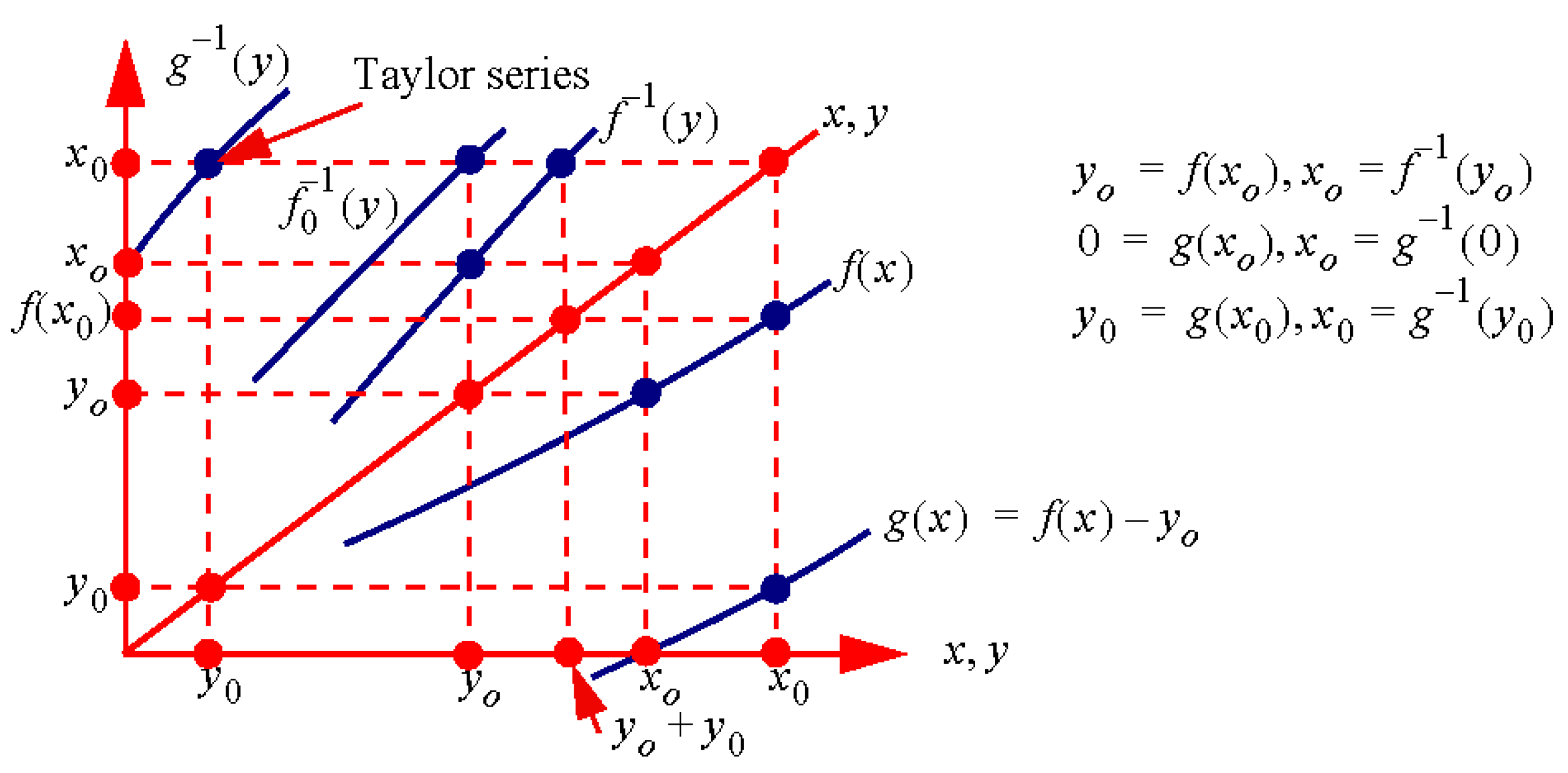
Consider the illustration, shown in Figure 1, of a function f and an initial approximation x 0 for the root of f , which is denoted as x o . The usual approach to finding a better approximation to x o than x 0 , is to utilize a first-order Taylor series approximation, denoted t 1 , for f which is based on the point x 0 , f ( x 0 ) . This leads to the classic Newton–Raphson approximation x 1 for the root x o according to
x 1 = x 0 f x 0 f 1 x 0
Naturally, and as illustrated in Figure 1, higher-order Taylor series are expected to lead to more accurate approximations. A second-order Taylor series yields the approximation
x 2 = x 0 f 1 x 0 f 2 x 0 · 1 ± 1 2 f x 0 f 2 x 0 f 1 x 0 2
Explicit higher-order approximations are increasingly problematic: the kth-order approximation is associated with the dominant root of a kth-order polynomial. This problem can be avoided by utilizing, as illustrated in Figure 1, Taylor series approximations, denoted as t k I (kth-order approximation), for the inverse function f 1 and based on the point y 0 , x 0 , y 0 = f x 0 . Whilst this may presuppose that the inverse function is known, the resulting Taylor series can be written solely in terms of f and known parameter values such as x 0 . Thus, this indirect approach leads to explicit analytical expressions for the root of f and for all orders of approximation, a preferable outcome. The details are noted below, and the result was proposed by Schröder in 1870 [12].

2.1. Schröder’s Approximations of the First Kind

Consider the nth-order Taylor series, denoted as t n I , for f 1 and based on the point y 0 , f 1 y 0 , where x 0 = f 1 y 0 :
t n I y = f 1 y 0 + y y 0 D f 1 y 0 + y y 0 2 2 · D 2 f 1 y 0 + +                                                                                         y y 0 n n ! · D n f 1 y 0
As f 1 y 0 = x 0 and y 0 = f x 0 , it then follows that the nth-order approximation to the root x o , as given by x n I = t n I 0 , is
  x n I = x 0 f ( x 0 ) D f 1 y 0 + f 2 x 0 2 · D 2 f 1 y 0 + +                                                                                                                                               1 n f n x 0 n ! · D n f 1 y 0                          
This is the basis of Schröder’s approximation of the first kind, e.g., [12] (Equation (21)), [11] (Equation (17)), [11] (Section 3) and [3] (Equation (20)).
Theorem 1.
Schröder’s Approximations of the First Kind. Consider a real function  f  that is strictly monotonic in the interval around a real root  x o  and including the initial approximation point of  x 0 . A nth-order Taylor series for  f 1  based on the point  y 0 , x 0 y 0 = f x 0 , yields the root according to
                      f 1 0 = x 0 + k = 1 n 1 k f k x 0 k ! · D k f 1 y 0 + ϵ n I ,     n 1,2 , , ϵ n I = 1 n + 1 y 0 n + 1 n + 1 ! · D n + 1 f 1 y k ,               y k 0 , y 0 ,                                
and the nth-order approximation to the root x o is
x n I = x 0 + k = 1 n 1 k f k x 0 k ! · D k f 1 y 0 ,             n 1,2 , .
Evaluation of the derivatives leads to the nth-order approximation defined by Schröder [12] (Equation (21)):
                                  x n I = x 0 f x 0 f 1 x 0 f 2 x 0 f 2 x 0   2 f 1 x 0 3 f 3 x 0 f 3 x 0   6 f 1 x 0 4 · 1 + 3 f 2 x 0 2     f 1 x 0 f 3 x 0 f 4 x 0 f 4 x 0   24 f 1 x 0 5 · 1 10 f 2 x 0 f 3 x 0     f 1 x 0 f 4 x 0 + 15 f 2 x 0 3     f 1 x 0 2 f 4 x 0 f 5 x 0 f 5 x 0   120 f 1 x 0 6 · 1 + 15 f 2 x 0 f 4 x 0     f 1 x 0 f 5 x 0 + 10 f 3 x 0 2     f 1 x 0 f 5 x 0 105 f 2 x 0 2 f 3 x 0     f 1 x 0 2 f 5 x 0 + 105 f 2 x 0 4     f 1 x 0 3 f 5 x 0 f 6 x 0 f 6 x 0   720 f 1 x 0 7 · 1 21 f 2 x 0 f 5 x 0     f 1 x 0 f 6 x 0 35 f 3 x 0 f 4 x 0     f 1 x 0 f 6 x 0 + 210 f 2 x 0 2 f 4 x 0     f 1 x 0 2 f 6 x 0 + 280 f 2 x 0 f 3 x 0 2     f 1 x 0 2 f 6 x 0 1260 f 2 x 0 3 f 3 x 0     f 1 x 0 3 f 6 x 0 + 945 f 2 x 0 5     f 1 x 0 4 f 6 x 0 + 1 n f n x 0 n ! · D n f 1 y 0
where
D n f 1 y = D n 1 1 f 1 f 1 y ,     D 1 f 1 y = 1 f 1 f 1 y .  
Proof. 
The general result for x n I follows from the above discussion. The form for the error ϵ n I is consistent with the Lagrange form for the error in an nth-order Taylor series approximation, e.g., [13] (p. 880, Equation (25.2.25)). The explicit form for x n I follows from the inverse function theorem and, for completeness, the evaluation of D k f 1 y 0 , k 1,2 , , 6 , is detailed in Appendix A. □

Notes

The convergence of an nth-order Schröder approximation is consistent with that of an nth-order Taylor series.
The first-order approximation is identical to the standard Newton–Raphson method result of
x 1 I = x 0 f x 0 f 1 x 0
The second-order approximation is
x 2 I = x 0 f x 0 f 1 x 0 f 2 x 0 f 2 x 0   2 f 1 x 0 3
and is a less complicated form than the second-order approximation specified by (4). This approximation is consistent with the second-order Adomian approximation for a root, e.g., [8].

2.2. Inverse Function Approximation

Consider the case of a well-defined function f whose inverse, f 1 , is unknown. For y o = f x o specified, the goal is to establish an approximation to x o = f 1 y o . As illustrated in Figure 2, the equivalent problem is that of finding the root of f x y o given an initial approximation to the root of x 0 . This is the basis for Schröder’s approximations for an inverse function.
Theorem 2.
Schröder-Based Approximations for an Inverse Function. Consider a real function  f   that is monotonic in the interval around a point  x 0  and including the associated root  x o  of  g x = f x y o . A nth-order Taylor series for  g 1 , based on the point  y 0 = f x 0 y o , yields
  f 1 y o = x 0 + k = 1 n 1 k f x 0 y o k k ! · D k f 1 f x 0 + ϵ n I y o ,     n 1,2 , , ϵ n I y o = 1 n + 1 f x 0 y o n + 1 n + 1 ! · D n + 1 f 1 y o + y k ,               y k 0 , y 0 ,                                
and the nth order approximation to  x o = f 1 y o  is
x n I = x 0 + k = 1 n 1 k f x 0 y o k k ! · D k f 1 f x 0 ,           n 1,2 , .
It then follows that the nth-order approximation for  f 1 y o , denoted  f n 1 y o , is
f n 1 y o = x 0 f x 0 y o f 1 x 0 f x 0 y o 2 f 2 x 0   2 f 1 x 0 3 f x 0 y o 3 f 3 x 0   6 f 1 x 0 4 · 1 + 3 f 2 x 0 2     f 1 x 0 f 3 x 0 f x 0 y o 4 f 4 x 0   24 f 1 x 0 5 · 1 10 f 2 x 0 f 3 x 0     f 1 x 0 f 4 x 0 + 15 f 2 x 0 3     f 1 x 0 2 f 4 x 0 f x 0 y o 5 f 5 x 0   120 f 1 x 0 6 · 1 + 15 f 2 x 0 f 4 x 0     f 1 x 0 f 5 x 0 + 10 f 3 x 0 2     f 1 x 0 f 5 x 0 105 f 2 x 0 2 f 3 x 0     f 1 x 0 2 f 5 x 0 + 105 f 2 x 0 4     f 1 x 0 3 f 5 x 0 f x 0 y o 6 f 6 x 0   720 f 1 x 0 7 · 1 21 f 2 x 0 f 5 x 0     f 1 x 0 f 6 x 0 35 f 3 x 0 f 4 x 0     f 1 x 0 f 6 x 0 + 210 f 2 x 0 2 f 4 x 0     f 1 x 0 2 f 6 x 0 + 280 f 2 x 0 f 3 x 0 2     f 1 x 0 2 f 6 x 0 1260 f 2 x 0 3 f 3 x 0     f 1 x 0 3 f 6 x 0 + 945 f 2 x 0 5     f 1 x 0 4 f 6 x 0 + 1 n f x 0 y o n n ! · D n f 1 f x 0
Proof. 
Whilst this result follows from Theorem 1 by considering f x y o rather than f x , it is informative to provide a direct proof: With g x = f x y o , it follows that g 1 0 = x o . Consider an initial approximation of x 0 to x o . The Taylor series approximation for g 1 at the point y 0 , x 0 , y 0 = f x 0 y o , is
t n I y = g 1 y 0 + y y 0 D g 1 y 0 + y y 0 2 2 · D 2 g 1 y 0 + +                                                                                                                                                                                     y y 0 n n ! · D n g 1 y 0
For the case of y = 0 , the definitions of g 1 y 0 = x 0 and y 0 = g x 0 = f x 0 y o yield the nth-order approximation, x n I , to x o according to
x n I = t n I 0 = x 0 f x 0 y o D g 1 y 0 + f x 0 y o 2 2 · D 2 g 1 y 0 + + 1 n f x 0 y o n n ! · D n g 1 y 0
and with an error given by
    ϵ n I y o = x o x n I = 1 n + 1 f x 0 y o n + 1 n + 1 ! · D n + 1 g 1 y k ,           y k 0 , y 0 .        
Consider the point x 0 and the definition of y 0 according to y 0 = g x 0 = f x 0 y o . Thus, y o + y 0 = f x 0 and, hence, x 0 = f 1 y o + y 0 = g 1 y 0 . It then follows, by considering the derivative of g 1 at the point y 0 , that
d d y g 1 y 0 = 1 g 1 ( x 0 ) x 0 = g 1 y 0 = 1 f 1 ( x 0 ) x 0 = f 1 y o + y 0                                               = d d y f 1 y o + y 0 = d d y f 1 f ( x 0                
and it then follows that
D ( k ) g 1 y 0 = D ( k ) f 1 f ( x 0 ,             k 1,2 , .
The required result, as stated by (14), then follows. □

2.3. Notes

Consider an initial approximation of f 0 1 for the inverse function f 1 . For a given value of y , the initial approximation of x 0 to f 1 y is given by f 0 1 ( y ) , and the first-order approximation for f 1 , consistent with (15), is
f 1 1 y = f 0 1 y f f 0 1 y y f 1 f 0 1 y
This result is identical to the approximation arising from the Newton–Raphson method. The second- and third-order approximations are:
f 2 1 y = f 0 1 y f f 0 1 y y f 1 f 0 1 y f f 0 1 y y 2 f 2 f 0 1 y   2 f 1 f 0 1 y 3
f 3 1 y = f 0 1 y f f 0 1 y y f 1 f 0 1 y f f 0 1 y y 2 f 2 f 0 1 y   2 f 1 f 0 1 y 3                   f f 0 1 y y 3 f 3 f 0 1 y   6 f 1 f 0 1 y 4 · 1 + 3 f 2 f 0 1 y 2     f 1 f 0 1 y f 3 f 0 1 y

2.4. Notes on Convergence

2.4.1. Convergence of Schröder Approximations

Consider the illustration of f , f 1 , g , g 1 and the initial approximation f 0 1 shown in Figure 2. For fixed y , with a value y o , the goal is for the initial approximation x 0 = f 0 1 ( y o ) to f 1 ( y o ) to yield a value of y 0 = g x 0 = f x 0 y o which is such that the region of convergence of the Taylor series approximation for g 1 , based on the point y 0 , includes the origin. When this is the case, convergence of the Schröder approximations is guaranteed at the point y o . The goal is for the initial approximation f 0 1 to be such that this is the case for all values of y o in the domain of f 1 .
To establish a bound for the region of convergence for a Taylor series for g 1 , consider the Taylor series for g based on the point x 0 and for g 1 based on the point y 0 :
y = g x 0 + x x 0 g ( 1 ) x 0 + x x 0 2 g 2 ( x 0 ) 2 + + x x 0 n g n x 0 n ! +           x = g 1 y 0 + y y 0 D g 1 y 0 + y y 0 2 D ( 2 ) g 1 ( y 0 ) 2 + +                                                                                                                                       y y 0 n D ( n ) g 1 ( y 0 ) n ! +
With the definitions
Δ y = y g x 0 = y y 0 , Δ x = x g 1 y 0 = x x 0 , c k = g k x 0 k ! , d k = D ( k ) g 1 ( y 0 ) k ! , k 1,2 , ,
it follows that
Δ y = c 1 Δ x + c 2 Δ x 2 + + c n Δ x n + Δ x = d 1 Δ y + d 2 Δ y 2 + + d n Δ y n +
Equality in the second equation depends on Δ y < r o c g 1 ( y 0 ) , where r o c g 1 is the region of convergence for the Taylor series of g 1 at the point y 0 . The following bound due to Landau, e.g., [14], is relevant:
r o c g 1 y 0 > r o c g ( x 0 ) 2 g ( 1 ) x 0 2 6 g m a x ( x 0 )
where r o c g ( x 0 ) is the region of convergence for the Taylor series for g at the point x 0 , g m a x is the maximum value of the magnitude of g within the region of convergence and g ( 1 ) x 0 is assumed to be non-zero.
Thus, the requirement for the initial approximation x 0 = f 0 1 ( y o ) to f 1 ( y o ) is for the associated value y 0 = f x 0 y o to have a magnitude that is less than the region of convergence for g 1 at the point y 0 . A sufficient condition is
y 0 < r o c g ( x 0 ) 2 g ( 1 ) x 0 2 6 g m a x ( x 0 )
The goal is for such a bound to hold for all values in the domain of the inverse function. The examples detailed below utilize initial approximations that lead to Schröder approximations with decreasing relative errors, which is indicative of convergence.

2.4.2. Relative Error Bound for First-Order Approximation

With an error ε 0 I ( y ) in the initial approximation f 0 1 ( y ) to f 1 y , i.e., f 1 y = f 0 1 y + ε 0 I ( y ) , it follows that the error, denoted as ε 1 I ( y ) and in the first-order approximation specified by (21), is
ε 1 I y = f 1 y f 1 1 y = ε 0 I y · ε 0 I y f 2 f 1 y 2 f 1 f 1 y ·                                                                                                                                             1 ε 0 I y f ( 3 ) f 1 y f 2 f 1 y 1 ε 0 I y f 2 f 1 y f 1 f 1 y + ε 0 I y 2 f 3 f 1 y 2 f 1 f 1 y
This result arises from the use of a second-order Taylor series for f f 0 1 y , and f ( 1 ) f 0 1 y , that are based on the point f 1 (y).
With the bound
ε 0 I y f 2 f 1 y 2 f 1 f 1 y < Δ 1 , y d o m a i n   o f   f 1 ,
the error for the first-order Schröder approximation is related to the error associated with the initial approximation f 0 1 according to
ε 1 I y < Δ 1 ε 0 I y
assuming the bracketed term in (29) is close to unity. With such approximations, the relationship between the relative error bounds of the original and the first-order Schröder approximations is
r e B , 1 < Δ 1 r e B , 0 .
The validity of this relationship depends on the nature of the function being approximated and the initial approximation being used. For example, this relationship is accurate for the approximations noted below for the inverse Langevin function but not for the approximations considered for arcsine.

2.5. Special Case: Ratio of Two Functions

Consider the case where f x = n ( x ) / d x is the ratio of two functions and the inverse f 1 is to be approximated. The following preliminary result facilitates this.
Lemma 1.
Higher-order Derivatives of Ratio of Two Functions. For the case where  f  is a differentiable function for all orders, and defined according to  f x = n ( x ) / d ( x ) , it is the case that
f k x = n k ( x ) d k + 1 ( x ) , n 1 x = d x n 1 x n ( x ) d 1 ( x ) n k x = d x n k 1 1 ( x ) k n k 1 ( x ) d 1 ( x )
Proof. 
The proof is detailed in Appendix B. □

Approximations for the Inverse of  f x = n ( x ) / d ( x )  

The iterative formula detailed in Lemma 1 is the basis for the explicit results detailed in Theorem 3.
Theorem 3.
Approximation for the inverse of f(x) = n(x)/d(x). For the case where  f  is differentiable, up to the order of approximation being considered, and monotonic in the interval of interest, the first- to fourth-order approximations for the inverse of  f x = n ( x ) / d ( x ) , based on an initial approximating function,  f 0 1 , are:
f 1 1 y = f 0 1 y n f 0 1 y y d f 0 1 y · d f 0 1 y n 1 f 0 1 y
f 2 1 y = f 0 1 y n f 0 1 y y d f 0 1 y · d f 0 1 y n 1 f 0 1 y n f 0 1 y y d f 0 1 y 2 · n 2 f 0 1 y d f 0 1 y 2 n 1 3 f 0 1 y
f 3 1 y = f 0 1 y n f 0 1 y y d f 0 1 y · d f 0 1 y n 1 f 0 1 y n f 0 1 y y d f 0 1 y 2 · n 2 f 0 1 y d f 0 1 y 2 n 1 3 f 0 1 y                                   n f 0 1 y y d f 0 1 y 3 · n 3 f 0 1 y d f 0 1 y 6 n 1 4 f 0 1 y · 1 + 3 n 2 2 f 0 1 y n 1 f 0 1 y n 3 f 0 1 y      
f 4 1 y = f 3 1 y n f 0 1 y y d f 0 1 y 4 · n 4 f 0 1 y d f 0 1 y 24 n 1 5 f 0 1 y ·   1 10 n 2 f 0 1 y n 3 f 0 1 y n 1 f 0 1 y n 4 f 0 1 y + 15 n 2 3 f 0 1 y n 1 2 f 0 1 y n 4 f 0 1 y
Proof. 
These results follow from Theorem 2 and the derivative results stated in Lemma 1 and Appendix C. □

2.6. Newton–Raphson Iteration

Given an initial approximation f 0 1 for f 1 , Newton–Raphson iteration yields the approximation f 1 1 , as specified by (21). Newton–Raphson iteration, based on f 1 1 , yields the second-order approximation
f 2 1 y = f 1 1 y f f 1 1 y y f 1 f 1 1 y                             = f 0 1 y f f 0 1 y y f 1 f 0 1 y f f 0 1 y f f 0 1 y y f 1 f 0 1 y y f 1 f 0 1 y f f 0 1 y y f 1 f 0 1 y
A third iteration yields:
f 3 1 y = f 2 1 y f f 2 1 y y f 1 f 2 1 y                               = f 0 1 y f f 0 1 y y f 1 f 0 1 y f f 0 1 y f f 0 1 y y f 1 f 0 1 y y f 1 f 0 1 y f f 0 1 y y f 1 f 0 1 y                                                             f f 0 1 y f f 0 1 y y f 1 f 0 1 y f f 0 1 y f f 0 1 y y f 1 f 0 1 y y f 1 f 0 1 y f f 0 1 y y f 1 f 0 1 y y f 1 f 0 1 y f f 0 1 y y f 1 f 0 1 y f f 0 1 y f f 0 1 y y f 1 f 0 1 y y f 1 f 0 1 y f f 0 1 y y f 1 f 0 1 y
and similarly for higher-order iteration. Note the complexity associated with functions of functions, which increases with iteration. For the convergent case, Newton–Raphson iteration exhibits quadratic convergence.

2.7. Notes

Whilst the geometry associated with the Newton–Raphson method for establishing an approximation to the root of a function is compelling, its natural generalization via higher-order Taylor series is problematic. In contrast, the indirect approach of utilizing a Taylor series based on the inverse function leads to explicit approximation expressions—Schröder’s approximations of the first kind—for all orders. There is pedagogical value in such an approach.
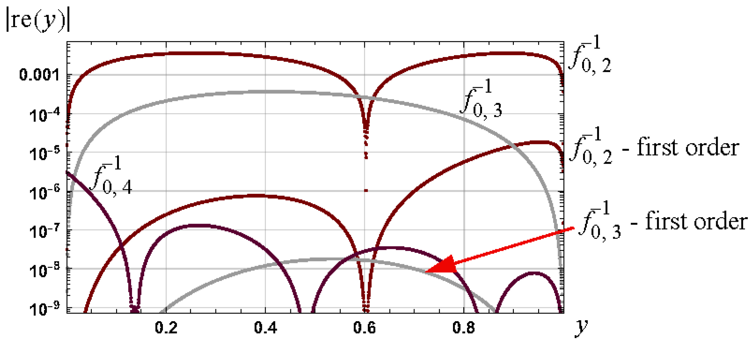
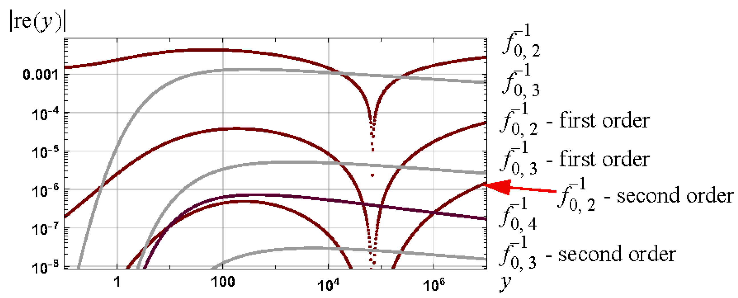
Figure 3 illustrates the potential interaction between high-order approximations, for example, via a high-order Schröder approximation, and utilizing iteration, for example, via Newton–Raphson iteration, to establish highly accurate analytical approximations for an inverse function given an initial low-accuracy approximation. A combination of a first-order Newton–Raphson iteration based on a modest-order Schröder approximation can lead to a good compromise between accuracy and complexity.
Note that a Schröder approximation is a means to establish a higher-accuracy approximation given an initial approximation with modest accuracy. The new improved approximation can then be used as the base approximation for Newton–Raphson iteration with, potentially, quadratic convergence.
The following four sections detail the establishment of accurate analytical approximations, based on initial approximations with modest relative error bounds, for arcsine, the inverse of x sin ( x ) , the inverse Langevin function and the Lambert W function.
In many instances, the initial approximation for the inverse function to be approximated is defined in a custom manner. Point-based approximations such as Taylor series expansions, for example, often do not lead to suitable initial approximations as such approximations of a fixed order, whilst having a low error at the point of approximation, generally have an increasing error, and potentially an increasing relative error, as the distance from the point of approximation increases. This situation is illustrated in Figure 2 of [15], where the relative errors in Taylor series approximations for arcsine are detailed.

3. Example I: Analytical Approximations for Arcsine

Given an approximation for arcsine, approximations for arccosine and arctangent readily follow from the relationships, e.g., [16] (p. 57, Equations (1.623) and (1.624)):
acos y = π 2 asin y , acos y = a s i n 1 y 2 , 0 y 1 ,
atan y = a s i n y 1 + y 2 = π 2 asin 1 1 + y 2 , 0 y < .
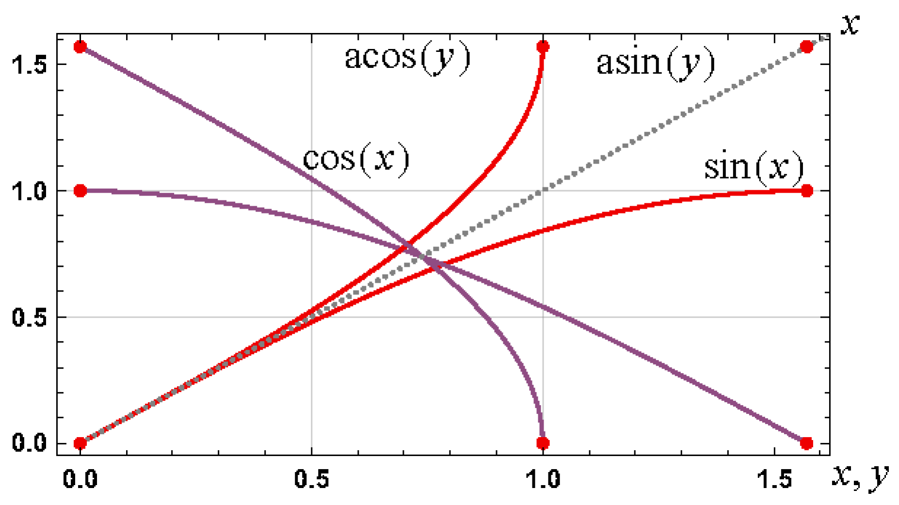
Naturally, there are many approximations for arcsine, and an overview of published approximations and new results for arcsine, arccosine and arctangent is provided in [15]. Graphs of arcsine and arccosine are shown in Figure 4.

3.1. General Schröder-Based Approximations

Consider y = f x = s i n ( x ) , 0 x < π / 2 and an initial approximation f 0 1 for the inverse function x = f 1 y = a s i n ( y ) , 0 y < 1 . Consistent with Theorem 2, the first- to fourth-order general approximations for arcsine are:
f 1 1 y = f 0 1 y sin f 0 1 y y c o s f 0 1 y
f 2 1 y = f 0 1 y sin f 0 1 y y c o s f 0 1 y + sin f 0 1 y sin f 0 1 y y 2 2 c o s f 0 1 y 3
f 3 1 y = f 0 1 y sin f 0 1 y y c o s f 0 1 y + sin f 0 1 y sin f 0 1 y y 2 2 c o s f 0 1 y 3       sin f 0 1 y y 3 6 c o s f 0 1 y 3 · 1 + 3 sin f 0 1 y 2 c o s f 0 1 y 2
f 4 1 y = f 0 1 y sin f 0 1 y y c o s f 0 1 y + sin f 0 1 y sin f 0 1 y y 2 2 c o s f 0 1 y 3 sin f 0 1 y y 3 6 c o s f 0 1 y 3 · 1 + 3 sin f 0 1 y 2 c o s f 0 1 y 2 + 3 sin f 0 1 y sin f 0 1 y y 4 8 c o s f 0 1 y 5 · 1 + 5 sin f 0 1 y 2 3 c o s f 0 1 y 2      

3.1.1. Initial Approximations

Consider the published approximations for arcsine [17], [15] (Equations (10) and (31)) and [13] (p. 81, Equation (4.4.46)):
f 0 , 1 1 y = π y 2 + 1 y 2
f 0 , 2 1 y = α 0 1 1 y + α 1 y + α 2 y 2 , α 0 = π 2 1306 10000 , α 1 = 10653 10000 π 4 , α 2 = π 4 9347 10000
f 0 , 3 1 y = π 2 π 2 4 π y + y 2 + c 2,3 y 3 + c 2,4 y 4 + c 2,5 y 5 c 2,3 = 16 3 + 6 π 5 π 2 2 , c 2,4 = 35 3 8 π + 15 π 2 4 , c 2,5 = 16 3 + 3 π 3 π 2 2
f 0 , 4 1 y = π 2 1 y · α 0 + α 1 y + α 2 y 2 + + α 7 y 7 α 0 = π 2 , α 1 = 0.2145988016 , α 2 = 0.0889789874 , α 3 = 0.0501743046 , α 4 = 0.0308918810 , α 5 = 0.0170881256 ,                         α 6 = 0.0066700901 , α 7 = 0.0012624911
which have the respective relative error bounds, for the interval 0 , 1 , of 4.72 × 10 2 , 3.62 × 10 3 , 3.64 × 10 4 and 3.04 × 10 6 .

3.1.2. Explicit Approximations

For example, the third approximation given by (48), when used in the general first- and second-order Schröder approximations specified by (42) and (43), yields the following approximations:
f 1 1 y = π 2 π 2 4 π y + y 2 + c 2,3 y 3 + c 2,4 y 4 + c 2,5 y 5                               cos π 2 4 π y + y 2 + c 2,3 y 3 + c 2,4 y 4 + c 2,5 y 5 y sin π 2 4 π y + y 2 + c 2,3 y 3 + c 2,4 y 4 + c 2,5 y 5
f 2 1 y = π 2 π 2 4 π y + y 2 + c 2,3 y 3 + c 2,4 y 4 + c 2,5 y 5                               cos π 2 4 π y + y 2 + c 2,3 y 3 + c 2,4 y 4 + c 2,5 y 5 y sin π 2 4 π y + y 2 + c 2,3 y 3 + c 2,4 y 4 + c 2,5 y 5 + cos π 2 4 π y + y 2 + c 2,3 y 3 + c 2,4 y 4 + c 2,5 y 5 cos π 2 4 π y + y 2 + c 2,3 y 3 + c 2,4 y 4 + c 2,5 y 5 y 2 2 sin π 2 4 π y + y 2 + c 2,3 y 3 + c 2,4 y 4 + c 2,5 y 5 3    
which have, respectively, relative error bounds of 1.78 × 10 8 and 3.68 × 10 12 for 0 y < 1 .

3.1.3. Results

The relative error bounds associated with the first- to fourth-order Schröder-based approximations, as specified by (42) to (45), are tabulated in Table 1 for the case of the initial approximations f 0 1 being specified by (46) to (49). The relative errors associated with the second, third and fourth approximations are illustrated in Figure 5.
From the results detailed in Table 1, and for a set initial approximation, the clear improvement achieved by utilizing a higher-order approximation form is evident. Also evident is the improvement, for a set order of approximation, achieved by utilizing an initial approximation with a lower relative error bound.

3.2. Newton–Raphson Iteration

Consider an initial approximation f 0 1 for arcsine. Consistent with (21), (38) and (39), Newton–Raphson iteration leads to the following result:
a s i n y = s 0 y + s 1 y + s 2 y + s i y = sin s 0 y + s 1 y + + s i 1 y y cos s 0 y + s 1 y + + s i 1 y ,                       i 1,2 , , s 0 y = f 0 1 y ,                                                  
where
s 1 y = sin f 0 1 y y cos f 0 1 y
s 2 y = sin f 0 1 y + s 1 y y cos f 0 1 y + s 1 y = sin f 0 1 y sin f 0 1 y y cos f 0 1 y y cos f 0 1 y sin f 0 1 y y cos f 0 1 y
s 3 y = sin f 0 1 y + s 1 y + s 2 y y cos f 0 1 y + s 1 y + s 2 y
s 4 y = sin f 0 1 y + s 1 y + s 2 y + s 3 y y cos f 0 1 y + s 1 y + s 2 y + s 3 y
Explicit general first-, second- and third-order approximations are:
f 1 1 y = f 0 1 y sin f 0 1 y y cos f 0 1 y
f 2 1 y = f 0 1 y sin f 0 1 y y cos f 0 1 y sin f 0 1 y sin f 0 1 y y cos f 0 1 y y cos f 0 1 y sin f 0 1 y y cos f 0 1 y
f 3 1 y = f 2 1 y sin f 0 1 y sin f 0 1 y y cos f 0 1 y sin f 0 1 y sin f 0 1 y y cos f 0 1 y y cos f 0 1 y sin f 0 1 y y cos f 0 1 y y cos f 0 1 y sin f 0 1 y y cos f 0 1 y sin f 0 1 y sin f 0 1 y y cos f 0 1 y y cos f 0 1 y sin f 0 1 y y cos f 0 1 y        
With f 0 1 specified by (46) to (49), the relative error bounds associated with these approximations are detailed in Table 1.

3.3. Hybrid Approximation

A first-order Newton–Raphson iteration, based on the second-order Schröder approximation f 2 1 as specified by (43), is
a s i n y f 2 1 y sin f 2 1 y y cos f 2 1 y   = f 0 1 y sin f 0 1 y y c o s f 0 1 y + sin f 0 1 y sin f 0 1 y y 2 2 c o s f 0 1 y 3                                         sin f 0 1 y sin f 0 1 y y c o s f 0 1 y + sin f 0 1 y sin f 0 1 y y 2 2 c o s f 0 1 y 3 y cos f 0 1 y sin f 0 1 y y c o s f 0 1 y + sin f 0 1 y sin f 0 1 y y 2 2 c o s f 0 1 y 3
For the case where f 0 1 , as defined by (48), is used in this equation, the relative error bound is 2.69 × 10 24 . Thus, an analytical approximation of modest complexity but with high accuracy. For comparison, f 0 1 , as defined by (48), has a relative error bound of 3.64 × 10 4 , and the associated second-order Schröder approximation (43) has a relative error bound of 3.68 × 10 12 .

3.4. Applications

3.4.1. Lower Bound

The approximation f 0 , 3 1 given by (48) is a lower bound for arcsine [15] (Equation (112)). Simulation results indicate that the first- to fourth-order approximations, as given by (42) to (45), and based on f 0 , 3 1 , are lower bounds with improved accuracy and with the relative error bounds detailed in Table 1. Thus, for example:
f 2 ( y ) a s i n ( y )
where f 2 is the second-order approximation defined by (51) and with a relative error bound of 3.68 × 10 12 . Upper bounded functions can be defined based on the lower bounded functions, as detailed in [18] (Lemma 1).

3.4.2. Integral

Consider the result
0 y a s i n t d t = 1 y 2 1 + y a s i n y , 0 < y < 1 .
It then follows, based on the first-order approximation given by (42), that
0 y a s i n t d t 1 y 2 1 + y f 0 1 y sin f 0 1 y y c o s f 0 1 y , 0 < y < 1 ,
for any function f 0 1 that is an approximation to arcsine. The use of the approximation f 0 , 3 1 (see (48)) in this equation yields the approximation, for 0 < y < 1 , of
0 y a s i n t d t 1 y 2 1 + π y 2 y π 2 4 π y + y 2 + c 2,3 y 3 + c 2,4 y 4 + c 2,5 y 5 y sin π 2 4 π y + y 2 + c 2,3 y 3 + c 2,4 y 4 + c 2,5 y 5 y 2 sin π 2 4 π y + y 2 + c 2,3 y 3 + c 2,4 y 4 + c 2,5 y 5
which has a relative error bound for the interval ( 0 , 1 ) of 3.66 × 10 8 .

4. Example II: Analytical Approximations for Inverse of x − Sin(x)

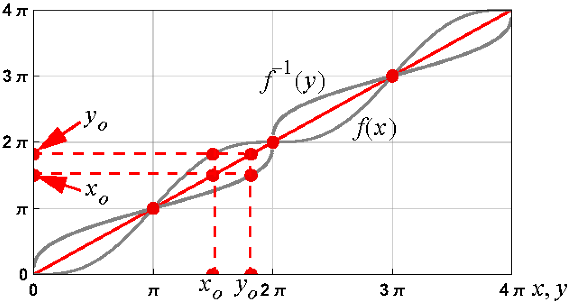
Whilst f x = x sin x is a simple elementary function, establishing its inverse is not straightforward as f 1 ( x ) = 0 , x 0 , 2 π , 4 π , , and derivatives of all orders of f 1 are undefined at the origin. Graphs of f and f 1 are shown in Figure 6.
As f x = x sin x is the summation of a linear function and a periodic function, and as it is anti-symmetric around the point π , π when considering the interval 0 , 2 π , it is sufficient to find an approximation for f 1 over the interval 0 , π . The proofs for the required results:
f 1 y = f 1 y 2 k π + 2 k π , 2 k π y < 2 k π + 2 π , f 1 y = 2 π f 1 2 π y , y π , 2 π ,
are detailed in Appendix D.

4.1. Initial Approximation for f 1

To define an initial approximation with a bounded relative error, consider a Taylor series at the origin for f x = x sin x which is
y = f x x 3 6 x 5 5 ! + x 7 7 ! +
By utilizing the first term in this series, an initial approximation for f 1 of
f 1 ( y ) 6 1 / 3 y 1 / 3
can be defined that is accurate for y 1 . An affine component can be added to this approximation to ensure equality of the new approximation to f 1 at the end point, π , of the interval of interest. As f 1 π = π , the approximation is
f 1 y c 0 y 1 / 3 + c 1 y , c 0 = 6 1 / 3 , c 1 = 1 6 1 / 3 π 2 / 3 ,
and has a relative error bound for the interval 0 , π of 1.89 × 10 2 . Some optimized generalizations are:
f 0 , 1 1 y = c 0 y 1 / 3 + c 1 y + c 22 y 2 π y , c 22 = 133 10000 ,
f 0 , 2 1 y = c 0 y 1 / 3 + c 1 y + c 32 y 2 π y + c 33 y 3 π y , c 32 = 305 10000 , c 33 = 105 10000 ,
f 0 , 3 1 y = c 0 y 1 / 3 + c 1 y + c 2 s i n ( y ) , c 2 = 449 10000 ,
with respective relative error bounds, for the interval 0 , π , of 8.61 × 10 3 , 5.74 × 10 3 and 1.36 × 10 3 .

4.2. General Schröder-Based Approximations

Consistent with Theorem 2, the first- to fourth-order approximations for f 1 over the interval 0 , π , and based on an initial approximation function of the form f 0 1 , are:
f 1 1 y = f 0 1 y f 0 1 y sin f 0 1 y y 1 cos f 0 1 y
f 2 1 y = f 0 1 y f 0 1 y sin f 0 1 y y 1 cos f 0 1 y         sin f 0 1 y f 0 1 y sin f 0 1 y y 2 2 1 cos f 0 1 y 3
  f 3 1 y = f 0 1 y f 0 1 y sin f 0 1 y y 1 cos f 0 1 y sin f 0 1 y f 0 1 y sin f 0 1 y y 2 2 1 cos f 0 1 y 3 + cos f 0 1 y f 0 1 y sin f 0 1 y y 3 6 1 cos f 0 1 y 4 · 1 3 sin f 0 1 y 2 cos f 0 1 y 1 cos f 0 1 y
f 4 1 y = f 0 1 y f 0 1 y sin f 0 1 y y 1 cos f 0 1 y sin f 0 1 y f 0 1 y sin f 0 1 y y 2 2 1 cos f 0 1 y 3 + cos f 0 1 y f 0 1 y sin f 0 1 y y 3 6 1 cos f 0 1 y 4 · 1 3 sin f 0 1 y 2 cos f 0 1 y 1 cos f 0 1 y +                   sin f 0 1 y f 0 1 y sin f 0 1 y y 4 24 1 cos f 0 1 y 5 · 1 + 10 cos f 0 1 y 1 cos f 0 1 y 15 sin f 0 1 y 2 1 cos f 0 1 y 2

Examples

Based on the approximation f 0 , 3 1 y specified in (71), the first- and second-order approximations for the interval 0 , π , and arising from (72) and (73), respectively, are:
f 1 y c 0 y 1 / 3 + c 1 y + c 2 s i n y                     c 0 y 1 / 3 + c 1 y + c 2 s i n y sin c 0 y 1 / 3 + c 1 y + c 2 s i n ( y ) y 1 cos c 0 y 1 / 3 + c 1 y + c 2 s i n ( y )
f 1 y c 0 y 1 / 3 + c 1 y + c 2 s i n y c 0 y 1 / 3 + c 1 y + c 2 s i n y sin c 0 y 1 / 3 + c 1 y + c 2 s i n ( y ) y 1 cos c 0 y 1 / 3 + c 1 y + c 2 s i n ( y ) sin c 0 y 1 / 3 + c 1 y + c 2 s i n ( y ) · c 0 y 1 / 3 + c 1 y + c 2 s i n y sin c 0 y 1 / 3 + c 1 y + c 2 s i n ( y ) y 2 2 1 cos c 0 y 1 / 3 + c 1 y + c 2 s i n ( y ) 3            
The respective relative error bounds associated with these approximations are 1.13 × 10 6 and 2.44 × 10 9 .

4.3. Newton–Raphson Iteration

Second-order Newton–Raphson iteration, consistent with (38) and based on the approximation f 0 1 ( y ) , yields the general approximation form
f 2 1 y = f 0 1 y f 0 1 y sin f 0 1 y y 1 cos f 0 1 y f 0 1 y f 0 1 y sin f 0 1 y y 1 cos f 0 1 y sin f 0 1 y f 0 1 y sin f 0 1 y y 1 cos f 0 1 y y 1 cos f 0 1 y f 0 1 y sin f 0 1 y y 1 cos f 0 1 y      
which has a relative error bound of 7.92 × 10 13 when the approximation specified in (71) is utilized for f 0 1 . The resulting approximation is of comparable complexity to the third-order Schröder approximation detailed in (74), which yields a similar relative error bound of 5.52 × 10 12 when the initial approximation specified in (71) is used.

4.4. Results

The relative error bounds associated with the approximations defined by (69) to (71) are tabulated in Table 2.
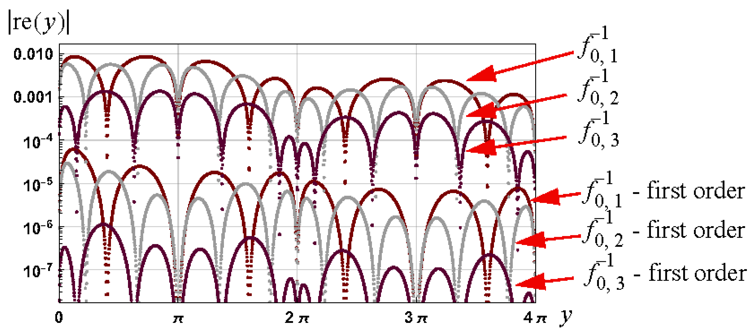
The relative error bounds over the intervals k π , ( k + 1 ) π , k { 1,2 , } , for the inverse of x s i n ( x ) , naturally, are lower. This is illustrated in Figure 7 where the relative errors for the approximations are shown over the interval 0 , 4 π .

4.5. Applications

The general integral formula for an inverse function (1) leads to
0 y f 1 λ d λ = y f 1 y f 1 y 2 2 cos f 1 y + 1
and approximations arise from utilizing a given approximation for f 1 . For example, the approximation f 0 , 3 1 defined by (71) leads to
0 y f 1 λ d λ y c 0 y 1 / 3 + c 1 y + c 2 s i n ( y ) 1 2 c 0 y 1 / 3 + c 1 y + c 2 s i n ( y ) 2 cos c 0 y 1 / 3 + c 1 y + c 2 s i n ( y ) + 1 , 0 < y π ,
which has a relative error bound of 3.20 × 10 6 for 0 , π . Second, the first-order approximation, as specified by (76), yields, for 0 < y π :
0 y f 1 λ d λ y c 0 y 1 / 3 + c 1 y + c 2 s i n y c 0 y 1 / 3 + c 1 y + c 2 s i n y sin c 0 y 1 / 3 + c 1 y + c 2 s i n ( y ) y 1 cos c 0 y 1 / 3 + c 1 y + c 2 s i n ( y ) 1 2 c 0 y 1 / 3 + c 1 y + c 2 s i n y c 0 y 1 / 3 + c 1 y + c 2 s i n y sin c 0 y 1 / 3 + c 1 y + c 2 s i n ( y ) y 1 cos c 0 y 1 / 3 + c 1 y + c 2 s i n ( y ) 2 cos c 0 y 1 / 3 + c 1 y + c 2 s i n y c 0 y 1 / 3 + c 1 y + c 2 s i n y sin c 0 y 1 / 3 + c 1 y + c 2 s i n ( y ) y 1 cos c 0 y 1 / 3 + c 1 y + c 2 s i n ( y ) + 1
which has a relative error bound of 2.23 × 10 12 for 0 , π .

5. Example III: Analytical Approximations for Inverse Langevin Function

The Langevin function is defined according to
y = L x = c o t h x 1 x , x ( 0 , ) 0 , x = 0 L x = L ( x )
and its inverse, L 1 , has been the subject of research interest over recent decades, e.g., [1,2]. Graphs of L and L 1 are shown in Figure 8 for the positive real line case. The use of the standard exponential definition for the hyperbolic cotangent function leads to
y = L x = x 1 + ( 1 + x ) e 2 x x 1 e 2 x = n ( x ) d ( x )
where n x = x 1 + ( 1 + x ) e 2 x and d x = x 1 e 2 x . This form implies, for fixed y , that x = L 1 ( y ) is the solution of
e 2 x = 1 x + x y 1 + x + x y

5.1. Approximations

For x , y small, a Taylor series approach, e.g., [19], yields the approximation
L 1 y 3 y + 9 y 3 5 + 297 y 5 175 + 1539 y 7 875 + , 0 y 1 .
For large x , consistent with y approaching one, the left-hand side in (84) becomes vanishingly small leading to the approximation
L 1 y 1 1 y , y 1 , y < 1 .
The issue, then, is how to incorporate both approximations into a simple expression that is valid for y 0 , 1 ) . Representative approximations for L 1 include:
L 0 , 1 1 y = 3 y 1 y · 1 24 y 25 + 22 y 2 75 ,
L 0 , 2 1 y = 3 y + y 2 5 · s i n 7 y 2 + y 3 1 y ,
L 0 , 3 1 y = y ( 3 y 2 ) 1 y 2 y 10 / 3 2 + 3 y 5 y 76 100 y 1 ,
and are defined, respectively, in [20,21,22]. Their respective relative error bounds, associated with the interval 0 , 1 ) , are: 9.69 × 10 3 , 1.79 × 10 3 and 7.22 × 10 4 . The papers [1,2,20,23,24], for example, detail alternative approximations.

5.2. General Schröder-Based Approximations

The general approximation forms for the inverse Langevin function that are detailed below are based on the form L x = n ( x ) / d ( x ) , as given by (83). The result for f k x = n k ( x ) d k + 1 ( x ) , stated in Lemma 1, yields the following results:
n 1 x = 1 2 e 2 x 4 x 2 e 2 x + e 4 x
n 2 x = 2 + 6 e 2 x + 8 x 3 e 2 x 6 e 4 x + 8 x 3 e 4 x + 2 e 6 x
n 3 x = 6 24 e 2 x 16 x 4 e 2 x + 36 e 4 x 64 x 4 e 4 x 24 e 6 x 16 x 4 e 6 x + 6 e 8 x
n 4 x = 24 + 120 e 2 x + 32 x 5 e 2 x 240 e 4 x + 352 x 5 e 4 x + 240 e 6 x + 352 x 5 e 6 x 120 e 8 x + 32 x 5 e 8 x + 24 e 10 x
These functions can be used in the general inverse function approximations stated in Theorem 3. With an initial approximation of f 0 1 , the first- and second-order approximations for L 1 are:
f 1 1 ( y ) = x 2 x + x y 2 x 2 + 2 x 2 + x y e 2 x + x 2 + x + x y e 4 x 1 2 e 2 x 4 x 2 e 2 x + e 4 x x = f 0 1 ( y )
f 2 1 ( y ) = 2 x n 1 3 x 2 n 1 2 x d x n x y d x n 2 x d ( x ) n x y d ( x ) 2 2 n 1 3 x x = f 0 1 ( y )
Higher-order approximations follow in a similar manner.

5.3. Results

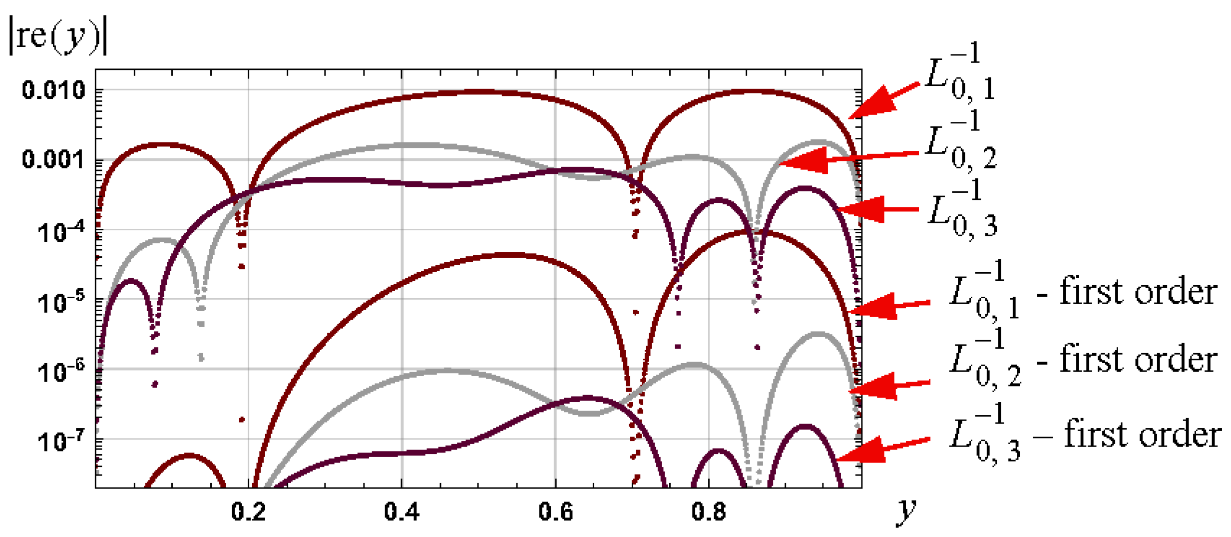
The relative error bounds, based on (87) to (89), for approximations to the inverse Langevin function are tabulated in Table 3. The relative errors associated with the original approximations, (87) to (89), and the associated first-order approximations (94) are shown in Figure 9.

5.4. Newton–Raphson Iteration

A second-order Newton–Raphson iteration, which is equivalent to a first-order Newton–Raphson iteration, based on the first-order approximation f 1 1 defined by (94), yields the approximation
f N R 2 1 y = f 1 1 y f f 1 1 y y f 1 f 1 1 y = f 1 1 y n f 1 1 y y d f 1 1 y d f 1 1 y n 1 f 1 1 y
For the case of initial approximations defined by (87) to (89), i.e.,
f 1 1 y = x 2 x + x y 2 x 2 + 2 x 2 + x y e 2 x + x 2 + x + x y e 4 x 1 2 e 2 x + 4 x 2 e 2 x + e 4 x x L 0 , 1 1 y , L 0 , 2 1 y , L 0 , 3 1 y
the relative error bounds for the interval 0 , 1 ) , respectively, are 8.80 × 10 9 , 1.03 × 10 11 and 1.09 × 10 13 .

5.5. Applications

As 0 x L λ d λ = ln s i n h ( x ) ln ( x ) , the general integral result, as given by (1), yields
0 y L 1 λ d λ = y L 1 y + ln L 1 y ln s i n h L 1 y , y 0 , 1 ,
and approximations then follow. For example, the approximation f 1 1   (see (94)) yields the relative error bounds for the integral of the inverse Langevin function, respectively, of 2.72 × 10 9 , 2.02 × 10 12 and 8.78 × 10 14 for the cases of f 0 1 specified by (87) to (89).
Direct integration of the original approximations, as given by (87) to (89), yields the approximations
0 y L 1 λ d λ y + y 2 22 y 3 75 ln 1 y ,
0 y L 1 λ d λ 16 1715 y + y 2 y 3 3 ln 1 y + 16 98 y 2 1715 · cos 7 y 2 + 8 y 245 · sin 7 y 2 ,
0 y L 1 λ d λ y 2 2 3 y 13 / 3 26 + 19 y 6 50 132 y 7 175 + 3 y 8 8 ln 1 y 2 ,
with relative error bounds of 6.43 × 10 3 , 1.14 × 10 3 and 5.34 × 10 4 . Use of the approximations, as given by (87) to (89), in (98) yields the respective relative error bounds of 6.71 × 10 5 , 2.22 × 10 6 and 3.25 × 10 7 .

Inverse Langevin Function as Zero Crossing Time of an Impulse Response

Rearranging (84) implies, for fixed y and 0 < y < 1 , that x = L 1 y is the solution of
1 x + x y 1 + x + x y e 2 x = 0 .
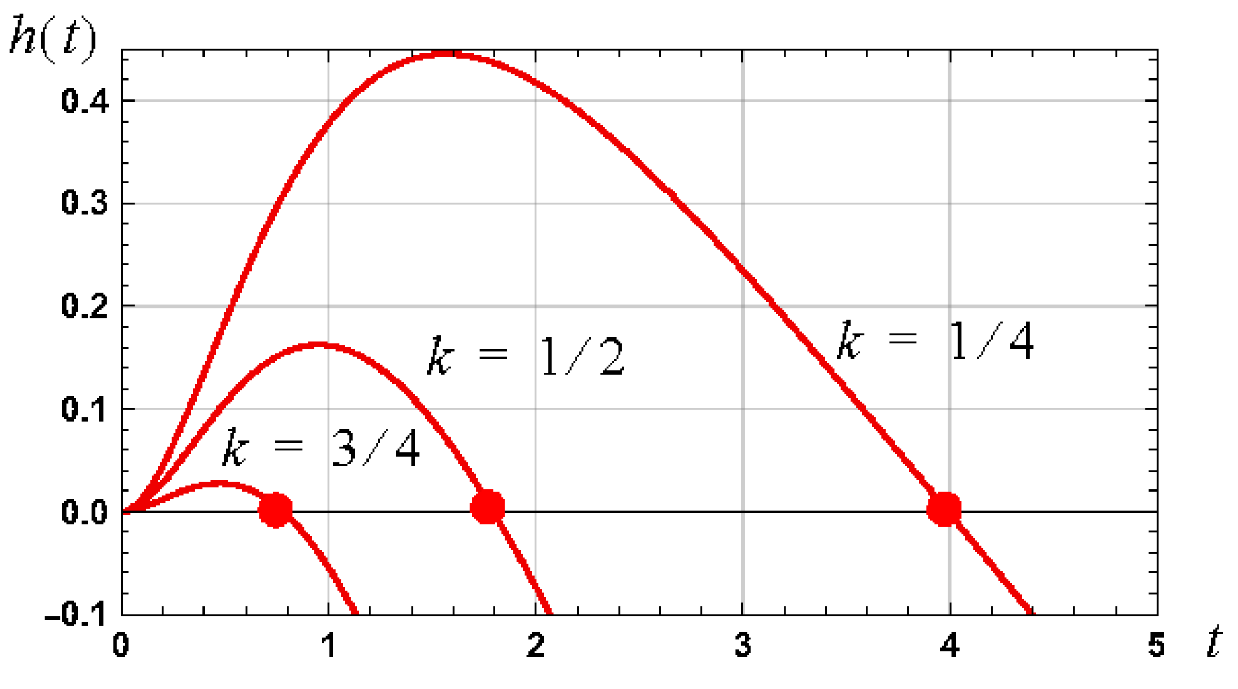
The function h t = 1 k t 1 + 2 k t e 2 t ,   t > 0 , arising from the definition of k = 1 y in this equation, is consistent with the impulse response of a linear system with a transfer function defined according to
H s = 1 s k s 2 1 / 2 1 + s / 2 1 k / 2 2 1 + s / 2 2
The zero crossing time of the impulse response is L 1 1 k for 0 < k < 1 . The impulse response is shown in Figure 10 for the cases of k 1 / 4 , 1 / 2 , 3 / 4 . The zero crossing times can be approximated via the approximations detailed above.

6. Example IV: Analytical Approximations for Lambert Function

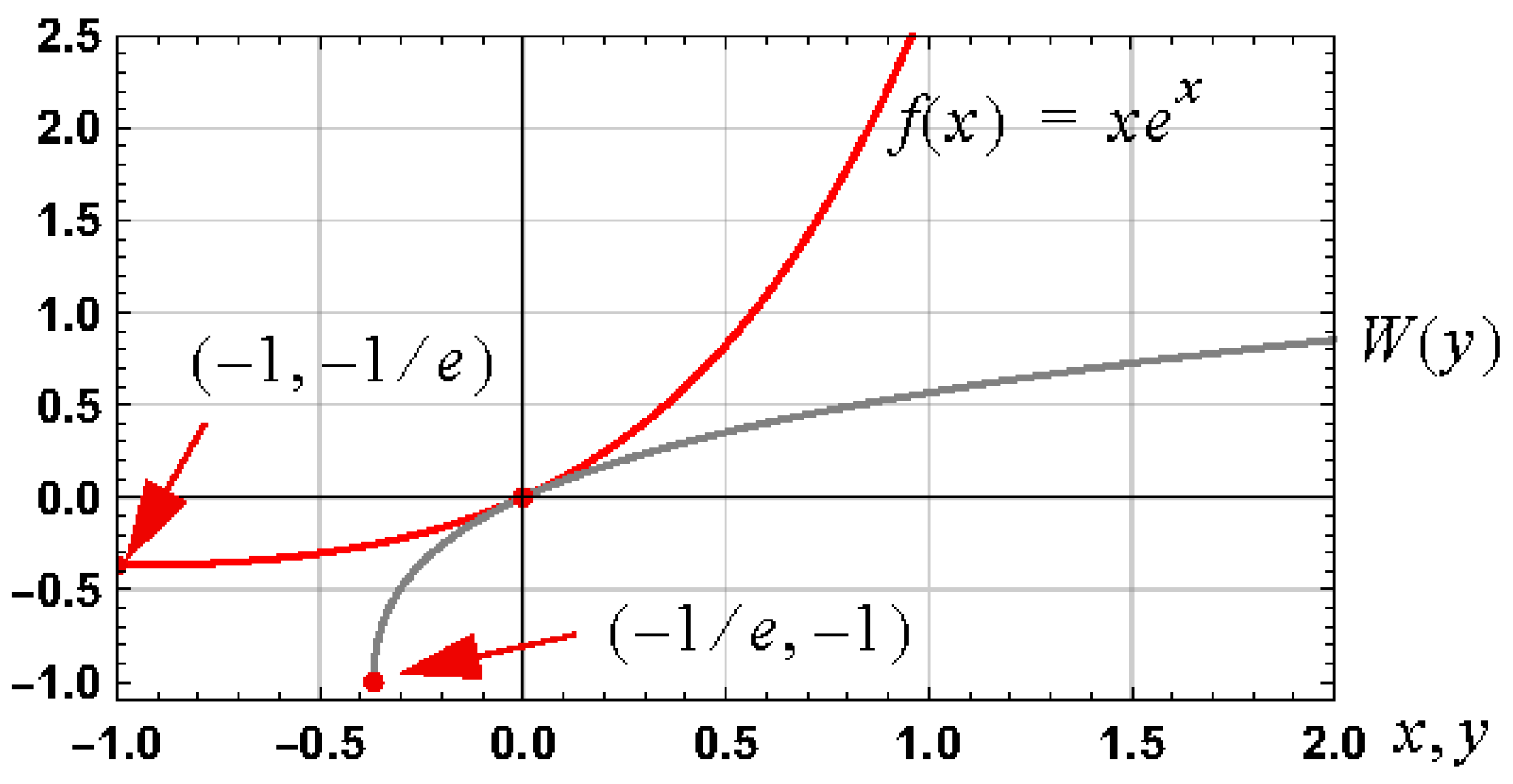
The Lambert W function, denoted W for the principle branch and real valued case, is a generalization of the logarithm function and its approximation has received increasing attention in the literature, e.g., [25,26,27]. It is defined as the inverse of y = f x = x e x for the case of x 1 , y 1 / e , i.e.,
x = W y = f 1 ( y )
A graph of the Lambert W function is shown in Figure 11.

6.1. Approximations

The Lambert W function has widespread applications, e.g., [28,29], and, accordingly, its approximation has received significant interest, with the following approximations, for example, being proposed:
f 0 , 1 1 y = ( 1 + δ ) ln 6 5 · y ln 12 5 · y ln 1 + 12 y / 5 δ ln 2 y ln 1 + 2 y δ = 0.4586887
f 0 , 2 1 y = 1 + a ln 1 + b 1 + e y 1 + c ln 1 + 1 + e y a = 2.036 , c = e 1 / a 1 2 / a 1 ln ( 2 ) e 1 / a , b = 2 a + c
f 0 , 3 1 y = ln 1 + 3 y + y ln 1 + y 1 + ln 1 + y 1 + ln 1 + 2 y 1 + ln 1 + y
f 0 , 4 1 y = ln 1 + 4 y + y ln 1 + 2 y 1 + ln 1 + y + y ln 1 + y 2 + ln 1 + 2 y 1 + ln 1 + y 1 + ln 1 + y 1 + ln 1 + 2 y 1 + ln 1 + y 1 + ln 1 + 3 y + y ln 1 + y 1 + ln 1 + y 1 + ln 1 + 2 y 1 + ln 1 + y        
These approximations, respectively, are defined by [30] (Equation (15)), [31] (Equations (19) and (20)), [26] (Equation (33)) and [26] (Equation (35)). The respective relative error bounds for these approximations, and for the interval 0 , ) , are: 1.96 × 10 3 , 4.53 × 10 3 , 1.33 × 10 3 and 7.22 × 10 7 . Useful overviews of published results can be found in [25,26,27,31,32].

6.2. General Schröder-Based Approximations

Based on the results stated in Theorem 2, the first- to fourth-order approximations for the Lambert W function, and based on an initial approximation of f 0 1 , are:
f 1 1 y = f 0 1 y f 0 1 y y e f 0 1 y 1 + f 0 1 y = f 0 1 y 2 + y e f 0 1 y 1 + f 0 1 y
f 2 1 y = f 0 1 y 2 + y e f 0 1 y 1 + f 0 1 y 2 + f 0 1 y f 0 1 y y e f 0 1 y 2 2 1 + f 0 1 y 3
f 3 1 y = f 0 1 y 2 + y e f 0 1 y 1 + f 0 1 y 2 + f 0 1 y f 0 1 y y e f 0 1 y 2 2 1 + f 0 1 y 3 3 + f 0 1 y f 0 1 y y e f 0 1 y 3 6 1 + f 0 1 y 4 · 1 + 3 2 + f 0 1 y 2 1 + f 0 1 y 3 + f 0 1 y
f 4 1 y = f 3 1 y 4 + f 0 1 y f 0 1 y y e f 0 1 y 4 24 1 + f 0 1 y 5 · 1 10 2 + f 0 1 y 3 + f 0 1 y 1 + f 0 1 y 4 + f 0 1 y 15 2 + f 0 1 y 3 1 + f 0 1 y 2 4 + f 0 1 y              

6.2.1. Special Form

For the case consistent with the approximations stated in (107) and (108), where
f 0 1 y = ln p ( y q ( y ,
the first- and second-order approximations, respectively, become
f 1 1 y = ln p ( y q ( y 2 + y q ( y ) p ( y ) 1 + ln p ( y q ( y
f 2 1 y = ln p ( y q ( y 2 + y q ( y ) p ( y ) 1 + ln p ( y q ( y 2 + ln p ( y q ( y ln p ( y q ( y y q ( y ) p ( y ) 2 2 1 + ln p ( y q ( y 3

6.2.2. Explicit Approximation

The use of f 0 , 3 1 y (see (107)) in the first-order form, as given by (109) or (114), yields the approximation
f 1 1 y = ln 1 + 3 y + y ln 1 + y 1 + ln 1 + y 1 + ln 1 + 2 y 1 + ln 1 + y 2 + y 1 + ln 1 + y 1 + ln 1 + 2 y 1 + ln 1 + y 1 + 3 y + y ln 1 + y 1 + ln 1 + 3 y + y ln 1 + y 1 + ln 1 + y 1 + ln 1 + 2 y 1 + ln 1 + y        
which has a relative error bound for 0 , of 5.12 × 10 6 .

6.3. Hybrid Approximations

Consider a first-order Newton–Raphson iteration based on the second-order approximation f 2 1 specified by (110), with f 0 1 defined by (107). The relative error bound associated with f 0 1 is 1.33 × 10 3 ; the relative error bound associated with f 2 1 is 2.93 × 10 8 . The first-order Newton–Raphson approximation is
W ( y )   f 2 1 y f 2 1 y y e f 2 1 y 1 + f 2 1 y
and has a relative error bound of 3.44 × 10 15 .

6.4. Results

The relative error bounds associated with Schröder and Newton–Raphson approximations are tabulated in Table 4. The relative errors for selected results are shown in Figure 12.

6.5. Applications

The approximations f 0 , 3 1 and f 0 , 4 1 , as given by (107) and (108), are upper bounds for the Lambert W function [26]. Simulation results indicate that the approximations, as given by (109) to (112), and based on these approximations, are also upper bounds with improved accuracy, and the bounds are detailed in Table 4. Lower bounded functions can be defined based on these upper bounds, as detailed in [18] (Lemma 1). Thus, for example, the second-order approximation given by (110) yields the bounds
1 1 + ε B f 0 1 y f 0 1 y y e f 0 1 y 1 + f 0 1 y 2 + f 0 1 y f 0 1 y y e f 0 1 y 2 2 1 + f 0 1 y 3 W ( y ) f 0 1 y f 0 1 y y e f 0 1 y 1 + f 0 1 y 2 + f 0 1 y f 0 1 y y e f 0 1 y 2 2 1 + f 0 1 y 3 f 0 1 f 0 , 3 1 , f 0 , 4 1
where ε B is the bound associated with the approximation and as given in Table 4. For example, when f 0 1 y is given by f 0 , 3 1 y (see (107)), ε B = 2.93 × 10 8 and the relative error bounds associated with the upper and lower bounded approximations are both 2.93 × 10 8 .
The general integral result given by (1), along with the integral result
0 y x e x d x = 1 + ( y 1 ) e y
yields
0 y f 1 ( λ ) d λ = y f 1 ( y ) + 1 f 1 ( y ) e f 1 ( y ) 1 , y > 0 ,
and approximations then follow. For example, the relative error bounds for the interval 0 , associated with directly utilizing the approximations specified by (105) to (108), respectively, are: 1.70 × 10 5 , 2.86 × 10 4 (for the interval 0 , 10 20 ), 6.17 × 10 6 and 1.81 × 10 12 . When the approximation f 1 1 (see (109)) is utilized, the relative error bounds for the integral of the Lambert W function, respectively, are 3.84 × 10 9 , 1.55 × 10 6 (for the interval 0 , 10 20 ), 1.11 × 10 10 and 8.37 × 10 24 for the cases of f 0 1 specified by (105) to (108). The integrals of the original approximations, as given by (105) to (108), are not known.

7. Conclusions

In this paper, Schröder approximations of the first kind, modified for the inverse function approximation case, were utilized to establish general analytical approximation forms for an inverse function. Such general forms can be used to establish arbitrarily accurate analytical approximations, with a set relative error bound, for an inverse function when an initial approximation, typically with low accuracy, is known. Approximations for arcsine, the inverse of x s i n ( x ) , the inverse Langevin function and the Lambert W function were used to illustrate the approach. Several applications were detailed.
Newton–Raphson iteration can also be used to yield analytical approximations to a given inverse function of arbitrary accuracy given an initial approximation with low to moderate accuracy but, in general, with a more complicated form. The use of a first-order Newton–Raphson iteration based on a Schröder approximation of a set order can lead to approximations that represent a good compromise between accuracy and complexity.
With respect to the root approximation of a function, Schröder approximations of the first kind, based on the inverse of a function, have an advantage over the corresponding generalization of the standard Newton–Raphson method, as explicit solutions for all orders of approximation can be obtained.

Further Research

The four examples considered illustrate the potential for utilizing Schröder approximations to establish accurate analytical approximations for an inverse function. As this approach is general, there is potential to establish useful analytical approximations for other inverse functions. The starting point is to find an initial approximation with a sufficiently low relative error bound over the domain of approximation. In general, custom approaches are used and advances in finding such approximations are of interest.
The relative error bound, as defined by (32), for the first-order Schröder approximation arises from two assumptions and the use of second-order Taylor series approximations that underpin (29). The use of first-order Taylor series leads, in general, to inaccurate results, and the complexity associated with the use of second-order Taylor series approximations complicates analysis. Further research to establish general relative error bounds, in terms of the relative bound of the initial approximation, for first-, second- and higher-order Schröder approximations is warranted.

Funding

This research did not receive external funding.

Acknowledgments

The author is pleased to acknowledge the support of A. Zoubir, SPG, Technische Universität Darmstadt, Darmstadt, Germany, who hosted a visit where part of the research underpinning this paper was completed. The author is appreciative of the feedback provided by the reviewers and the Academic Editor, which has led to an improved paper.

Conflicts of Interest

The author declares no conflict of interest.

Appendix A. Proof of Theorem 1

Useful references include [33] and the Faà die Bruno formula, e.g., [34]. A direct proof follows from the inverse function theorem, which states, for a real, monotonic and differentiable function, that
D f 1 ( y ) = 1 f 1 ( x ) x = f 1 ( y ) = 1 f 1 f 1 ( y )
Successive differentiation and use of the chain rule yield:
D ( 2 ) f 1 ( y ) = f 2 ( x ) f 1 ( x ) 3 x = f 1 ( y )
D ( 3 ) f 1 ( y ) = f 3 ( x ) f 1 ( x ) 4 + 3 f 2 ( x ) 2 f 1 ( x ) 5 x = f 1 ( y )
D ( 4 ) f 1 ( y ) = f 4 ( x ) f 1 ( x ) 5 + 10 f 2 ( x ) f 3 ( x ) f 1 ( x ) 6 15 f 2 ( x ) 3 f 1 ( x ) 7 x = f 1 ( y )
D ( 5 ) f 1 ( y ) = f 5 ( x ) f 1 ( x ) 6 + 15 f 2 ( x ) f 4 ( x ) f 1 ( x ) 7 + 10 f 3 x 2 f 1 x 7                               105 f 2 x 2 f 3 x f 1 x 8 + 105 f 2 x 4 f 1 x 9 x = f 1 y                  
D ( 6 ) f 1 ( y ) = f 6 ( x ) f 1 ( x ) 7 + 21 f 2 ( x ) f 5 ( x ) f 1 ( x ) 8 + 35 f 3 ( x ) f 4 ( x ) f 1 ( x ) 8 210 f 2 x 2 f 4 x f 1 x 9                 280 f 2 x f 3 x 2 f 1 x 9 + 1260 f 2 x 3 f 3 x f 1 x 10 945 f 2 x 5 f 1 x 11 x = f 1 y                  

Appendix B. Proof of Lemma 1

A general formula for f ( k ) , where f x = n ( x ) / d ( x ) , can be obtained from Leibniz’s rule for differentiation of the product of two functions, see, for example, [35]. The proof for the stated iterative algorithm follows from the differentiation of f x = n ( x ) / d ( x ) , which yields
f 1 x = n 1 x d x d 1 x n x d 2 ( x ) = n 1 ( x ) d 2 ( x )
where n 1 x = d x n 1 x n x d 1 x . Differentiation of f ( 1 ) yields
f 2 x = n 1 ( 1 ) x d x 2 d 1 x n 1 x d 3 ( x ) = n 2 ( x ) d 3 ( x )
where n 2 x = d x n 1 ( 1 ) x 2 n 1 x d 1 x . Differentiation of f ( 2 ) yields
f 3 x = n 2 ( 1 ) x d x 3 d 1 x n 2 x d 4 ( x ) = n 3 ( x ) d 4 ( x )
where n 3 x = d x n 2 ( 1 ) x 3 n 2 x d 1 x . The required general relationship of
f k x = n k ( x ) d k + 1 ( x ) , n k x = d x n k 1 ( 1 ) x k n k 1 x d 1 x ,
then follows.

Appendix C. Derivative of f ( k ) for the Case of f x = n ( x ) d ( x )

With f x = n ( x ) d ( x ) , the result f k x = n k ( x ) d k + 1 ( x ) , stated in Lemma 1, yields the following results for the derivatives of f 1 :
D f 1 ( y ) = 1 f 1 ( x ) x = f 1 ( y ) = d 2 ( x ) n 1 ( x ) x = f 1 ( y )
D ( 2 ) f 1 ( y ) = f 2 ( x ) f 1 ( x ) 3 x = f 1 ( y ) = d 3 ( x ) n 1 3 ( x ) · n 2 ( x ) x = f 1 ( y )
D ( 3 ) f 1 ( y ) = d 4 ( x ) n 1 4 ( x ) · n 3 ( x ) · 1 3 n 2 2 ( x ) n 1 ( x ) n 3 ( x ) x = f 1 ( y )
D ( 4 ) f 1 ( y ) = d 5 ( x ) n 1 5 ( x ) · n 4 ( x ) · 1 10 n 2 x n 3 x n 1 x n 4 x + 15 n 2 3 ( x ) n 1 2 ( x ) n 4 ( x ) x = f 1 ( y )
D ( 5 ) f 1 ( y ) = d 6 ( x ) n 1 6 ( x ) · n 5 ( x ) · 1 15 n 2 x n 4 x n 1 x n 5 x 10 n 3 2 x n 1 x n 5 x + 105 n 2 2 ( x ) n 3 x n 1 2 ( x ) n 5 x 10⁵ n 2 4 ( x ) n 1 3 ( x ) n 5 ( x ) x = f 1 ( y )

Appendix D. Inverse of x-Sin(x): Use of Periodicity and Anti-Symmetry
Establishing the inverse of f x = x s i n ( x ) is facilitated by the following two results:
Lemma 2.
Inverse of a Function Comprising a Linear and a Periodic Component. Consider a function  f  that is monotonically increasing from zero and comprises a linear component plus a periodic component, with a period,  x p , such that
f x = β x + f p x , f p x = f p x + k x p ,   f p x = 0 , k 0 , 1 , 2 , , x > 0 .                      
For the case of  x 1 = x + k x p 0 x < x p k 0 , 1 , 2 , , it follows that
y 1 = f x 1 = f x + k x p = k β x p + f x = y + k y p ,
where  y p = β x p  and  y = f ( x ) . The inverse function then satisfies the relationship
f 1 y + k y p = f 1 y + k y p β , 0 y < y p , k 0 , 1 , 2 , .
For the case of  f x = x s i n ( x ) , consistent with  β = 1 x p = 2 π  and  y p = 2 π , it follows that
f 1 y = f 1 y 2 k π + 2 k π , 2 k π y < 2 k π + 2 π .
Proof. 
The first result follows very simply:
f x + k x p = β x + k x p + f p x + k x p = k β x p + f x .
The second result follows from the definitions y 1 = y + k y p , x 1 = x + k x p , x 1 = f 1 y 1 and x = f 1 ( y ) , which imply that
x 1 = f 1 y 1 = f 1 y + k y p , x 1 = x + k x p = f 1 y + k y p β .
Equating these two results yields the required result: f 1 y + k y p = f 1 y + k y p β .
For the case of f x = x s i n ( x ) , consistent with β = 1 , x p = 2 π and y p = 2 π , it follows that
f 1 z + 2 k π = f 1 z + 2 k π , 0 z < 2 π , f 1 y = f 1 y 2 k π + 2 k π , 2 k π y < 2 k π + 2 π ,
assuming z = y 2 k π .  □
Lemma 3.
Use of Anti-Symmetric Nature of f in Defining f−1. For the case of  f x = x s i n ( x ) , which is antisymmetric over the interval  0 , 2 π  and around the point  π , π , it follows that
f x = 2 π f 2 π x , x π , 2 π ,
f 1 y = 2 π f 1 2 π y , y π , 2 π .
Proof. 
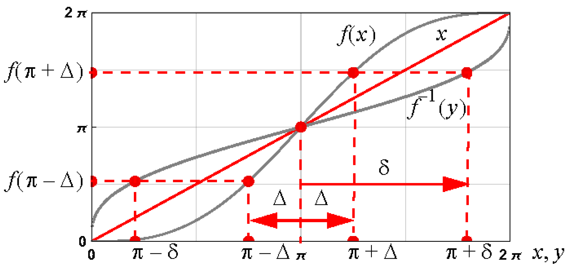
Consider the illustration shown in Figure A1. From the definition f x = x s i n ( x ) , it follows that
f π + Δ = π + Δ + sin Δ , f π Δ = π Δ sin Δ , Δ 0 , π .
Thus, f π + Δ + f π Δ = 2 π , and with x = π + Δ   x π , 2 π , the first result f x = 2 π f 2 π x , x π , 2 π , follows.
In a similar manner, consider δ , δ 0 , π , such that f 1 π + δ = f π + Δ and f 1 π δ = f π Δ . It then follows that
f 1 π + δ = π + Δ + sin Δ , f 1 π δ = π Δ sin Δ , Δ , δ 0 , π
Thus, f 1 π + δ + f 1 π δ = 2 π . With y = π + δ , y π , 2 π , the second required result
f 1 y = 2 π f 1 2 π y
follows. □
Figure A1. Illustration of the definitions Δ and δ and the anti-symmetric nature of f and f 1 around the point π , π .
Axioms 12 01042 g0a1

References

  1. Jedynak, R. New facts concerning the approximation of the inverse Langevin function. J. Non-Newtonian Fluid Mech. 2017, 249, 8–25. [Google Scholar] [CrossRef]
  2. Jedynak, R. A comprehensive study of the mathematical methods used to approximate the inverse Langevin function. Math. Mech. Solids 2018, 24, 1992–2016. [Google Scholar] [CrossRef]
  3. Gdawiec, K.; Kotarski, W.; Lisowska, A. Polynomiography based on the nonstandard Newton-like root finding methods. Abstr. Appl. Anal. 2015, 2015, 797594. [Google Scholar] [CrossRef]
  4. Ypma, T.J. Historical development of the Newton–Raphson method. SIAM Rev. 1995, 37, 531–551. [Google Scholar] [CrossRef]
  5. Kalantari, B.; Kalantari, I.; Zaare-Nahandi, R. A basic family of iteration functions for polynomial root finding and its characterizations. J. Comput. Appl. Math. 1997, 80, 209–226. [Google Scholar] [CrossRef]
  6. Petković, M.; Herceg, D. On rediscovered iteration methods for solving equations. J. Comput. Appl. Math. 1999, 107, 275–284. [Google Scholar] [CrossRef]
  7. Amat, S.; Busquier, S.; Gutiérrez, J.M. Geometric constructions of iterative functions to solve nonlinear equations. J. Comput. Appl. Math. 2003, 157, 197–205. [Google Scholar] [CrossRef]
  8. Abbasbandy, S. Improving Newton–Raphson method for nonlinear equations by modified Adomian decomposition method. Appl. Math. Comput. 2003, 145, 887–893. [Google Scholar] [CrossRef]
  9. Chun, C. Iterative methods improving Newton’s method by the decomposition method. Comput. Math. Appl. 2005, 50, 1559–1568. [Google Scholar] [CrossRef]
  10. Noor, M.A.; Gupta, V. Modified Householder iterative method free from second derivatives for nonlinear equations. Appl. Math. Comput. 2007, 190, 1701–1706. [Google Scholar] [CrossRef]
  11. Dubeau, F. Polynomial and rational approximations and the link between Schröder’s processes of the first and second kind. Abstr. Appl. Anal. 2014, 2014, 719846. [Google Scholar] [CrossRef]
  12. Schröder, E. Über unendlich viele Algorithmen zur Auflösung der Gleichungen. Math. Ann. 1870, 2, 317–365. [Google Scholar] [CrossRef]
  13. Abramowitz, M.; Stegun, I.A. (Eds.) Handbook of Mathematical Functions with Formulas, Graphs and Mathematical Tables; Dover: Mineola, NY, USA, 1964. [Google Scholar]
  14. Copson, E.T. An Introduction to the Theory of Functions of a Complex Variable; Oxford University Press: Oxford, UK, 1935; pp. 121–123. [Google Scholar]
  15. Howard, R.M. Radial Based Approximations for Arcsine, Arccosine, Arctangent and Applications. AppliedMath 2023, 3, 343–394. [Google Scholar] [CrossRef]
  16. Gradshteyn, I.S.; Ryzhik, I.M. Tables of Integrals, Series and Products, 7th ed.; Jeffery, A., Zwillinger, D., Eds.; Academic Press: Cambridge, MA, USA, 2007. [Google Scholar]
  17. Fink, A.M. Two inequalities. Univ. Beograd. Publ. Elektrotehn. Fak. Ser. Mat. 1995, 6, 49–50. [Google Scholar]
  18. Howard, R.M. Arbitrarily accurate analytical approximations for the Error function. Math. Comput. Appl. 2022, 27, 14. [Google Scholar] [CrossRef]
  19. Itskov, M.; Dargazany, R.; Hornes, K. Taylor expansion of the inverse function with application to the Langevin function. Math. Mech. Solids 2011, 17, 693–701. [Google Scholar] [CrossRef]
  20. Howard, R.M. Analytical approximations for the inverse Langevin function via linearization, error approximation and iteration. Rheol. Acta 2020, 59, 521–544. [Google Scholar] [CrossRef]
  21. Petrosyan, R. Improved approximations for some polymer extension models. Rheol. Acta 2017, 56, 21–26. [Google Scholar] [CrossRef]
  22. Nguessong, A.N.; Beda, T.; Peyraut, F. A new based error approach to approximate the inverse Langevin function. Rheol. Acta 2014, 53, 585–591. [Google Scholar] [CrossRef]
  23. Kröger, M. Simple, admissible, and accurate approximants of the inverse Langevin and Brillouin functions, relevant for strong polymer deformations and flows. J. Non-Newton. Fluid Mech. 2015, 223, 77–87. [Google Scholar] [CrossRef]
  24. Marchi, B.C.; Arruda, E.M. Generalized error-minimizing, rational inverse Langevin approximations. Math. Mech. Solids 2019, 24, 1630–1647. [Google Scholar] [CrossRef]
  25. Veberič, D. Lambert W function for applications in physics. Comput. Phys. Commun. 2012, 183, 2622–2628. [Google Scholar] [CrossRef]
  26. Howard, R.M. Analytical approximations for the principal branch of the Lambert W function. Eur. J. Math. Anal. 2022, 2, 14. [Google Scholar] [CrossRef]
  27. Lóczi, L. Guaranteed-and high-precision evaluation of the Lambert W function. Appl. Math. Comput. 2022, 433, 127406. [Google Scholar] [CrossRef]
  28. Banwell, T.C. Bipolar transistor circuit analysis using the Lambert W-function. IEEE Trans. Circuits Syst. I Fundam. Theory Appl. 2000, 47, 1621–1633. [Google Scholar] [CrossRef]
  29. Visser, M. Primes and the Lambert W function. Mathematics 2018, 6, 56. [Google Scholar] [CrossRef]
  30. Barry, D.A.; Parlange, J.Y.; Li, L.; Prommer, H.; Cunningham, C.J.; Stagnitti, F. Analytical approximations for real values of the Lambert W-function. Math. Comput. Simul. 2000, 53, 95–103. [Google Scholar] [CrossRef]
  31. Iacono, R.; Boyd, J.P. New approximations to the principal real-valued branch of the Lambert W-function. Adv. Comput. Math. 2017, 43, 1403–1436. [Google Scholar] [CrossRef]
  32. Goličnik, M. On the Lambert W function and its utility in biochemical kinetics. Biochem. Eng. J. 2012, 63, 116–123. [Google Scholar] [CrossRef]
  33. Dargazany, R.; Hörnes, K.; Itskov, M. A simple algorithm for the fast calculation of higher order derivatives of the inverse function. Appl. Math. Comput. 2013, 221, 833–838. [Google Scholar] [CrossRef]
  34. Craik, A.D. Prehistory of Faà di Bruno’s formula. Am. Math. Mon. 2005, 112, 119–130. [Google Scholar]
  35. Leslie, R.A. How not to repeatedly differentiate a reciprocal. Am. Math. Mon. 1991, 98, 732–735. [Google Scholar] [CrossRef]
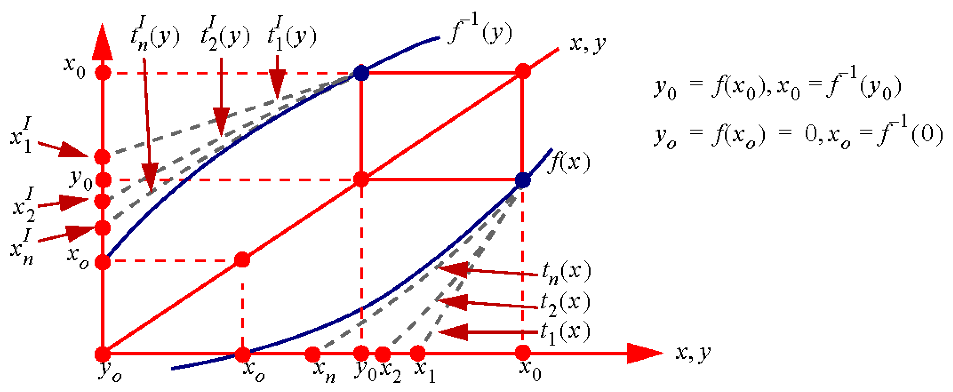
Figure 1. Illustration of the functions y = f x and x = f 1 y and Taylor series approximations to these functions based on the points x 0 , f ( x 0 ) and y 0 , f 1 y 0 . The root of the Taylor series, denoted, respectively, x 1 , x 2 , , x n and x 1 I , x 2 I , , x n I , are approximations for the roots of f .
Axioms 12 01042 g001
Figure 2. Illustration of the root of f x y o , denoted x o and given by f 1 y o , and an initial approximation of x 0 to x o . The illustration is for the monotonically increasing function case. The function f 0 1 is an initial approximation to f 1 .
Axioms 12 01042 g002
Figure 3. Illustration of the interaction between direct high order approximation, and iteration, to obtain accurate analytical inverse function approximations.
Axioms 12 01042 g003
Figure 4. Graph of y = f x = sin x , x = f 1 y = asin y , y = g x = cos x and x = g 1 y = acos y for 0 x < π / 2 , 0 y < 1 .
Axioms 12 01042 g004
Figure 5. Graph of the relative errors in approximations to a s i n ( y ) .
Axioms 12 01042 g005
Figure 6. Graphs of f x = x sin x and its inverse f 1 ( y ) .
Axioms 12 01042 g006
Figure 7. Graph of the relative error in approximations to the inverse of x s i n ( x ) . Upper three curves: original approximations defined by (69) to (71). Lower three curves: first order approximation as defined by (72).
Axioms 12 01042 g007
Figure 8. Graph of the Langevin and inverse Langevin functions.
Axioms 12 01042 g008
Figure 9. Graph of the relative error in approximations to the inverse Langevin function. Upper three curves: original approximations as given by (87) to (89). Lower three curves: associated first order approximations as specified by (94).
Axioms 12 01042 g009
Figure 10. Graph of the impulse response of the transfer function defined by (103).
Axioms 12 01042 g010
Figure 11. Graph of f x = x e x and its inverse, the Lambert W function, denoted W , for the principle branch and real case.
Axioms 12 01042 g011
Figure 12. Graphs of the relative error in approximations to the Lambert W function.
Axioms 12 01042 g012
Table 1. Relative error bounds, over the interval 0 , 1 , for approximations to arcsine based on the original approximations f 0 , 1 1 , f 0 , 2 1 , f 0 , 3 1 and f 0 , 4 1 , as specified by (46) to (49).
Approximation f 0 , 1 1 f 0 , 2 1 f 0 , 3 1 f 0 , 4 1
Original approximation 4.72 × 10 2 3.62 × 10 3 3.64 × 10 4 3.04 × 10 6
1st order: (42) 1.96 × 10 3 1.84 × 10 5 1.78 × 10 8 9.18 × 10 16
2nd order: (43) 3.39 × 10 4 2.46 × 10 7 3.68 × 10 12 4.43 × 10 22
3rd order: (44) 8.93 × 10 5 4.43 × 10 9 7.22 × 10 16 1.27 × 10 30
4th order: (45) 2.91 × 10 5 9.37 × 10 11 1.71 × 10 19 3.44 × 10 37
5th order 1.08 × 10 5 2.18 × 10 12 4.26 × 10 23 1.95 × 10 45
NR—1st iteration: (57) 1.96 × 10 3 1.84 × 10 5 1.78 × 10 8 9.18 × 10 16
NR—2nd iteration: (58) 1.28 × 10 5 8.87 × 10 10 6.52 × 10 17 4.94 × 10 32
NR—3rd iteration: (59) 1.29 × 10 9 3.54 × 10 18 1.05 × 10 33 1.12 × 10 63
NR—4th iteration 2.76 × 10 17 9.56 × 10 35 2.92 × 10 67 2.70 × 10 126
Table 2. Relative error bounds, over the interval 0 , π , for approximations to the inverse of x s i n ( x ) and based on the original approximations f 0 , 1 1 , f 0 , 2 1 and f 0 , 3 1 as defined by (69) to (71).
Approximation f 0 , 1 1 f 0 , 2 1 f 0 , 3 1
Original approximation 8.61 × 10 3 5.74 × 10 3 1.36 × 10 3
1st order: (72) 6.13 × 10 5 2.93 × 10 5 1.13 × 10 6
2nd order: (73) 8.24 × 10 7 2.67 × 10 7 2.44 × 10 9
3rd order: (74) 1.31 × 10 8 2.91 × 10 9 5.52 × 10 12
4th order: (75) 2.28 × 10 10 3.49 × 10 11 1.42 × 10 14
5th order 4.23 × 10 12 4.43 × 10 13 3.83 × 10 17
NR—1st iteration: (72) 6.13 × 10 5 2.93 × 10 5 1.13 × 10 6
NR—2nd iteration: (78) 3.18 × 10 9 7.69 × 10 10 7.92 × 10 13
NR—3rd iteration 8.61 × 10 18 5.31 × 10 19 3.95 × 10 25
NR—4th iteration 6.31 × 10 35 2.54 × 10 37 9.89 × 10 50
Table 3. Relative error bounds over the interval 0 , 1 ) for approximations to the inverse Langevin function based on the original approximations L 0 , 1 1 , L 0 , 2 1 and L 0 , 3 1 , as given by (87) to (89).
Approximation L 0 , 1 1 L 0 , 2 1 L 0 , 3 1
Original approximation 9.69 × 10 3 1.79 × 10 3 7.22 × 10 4
1st order: (94) 9.39 × 10 5 3.20 × 10 6 3.81 × 10 7
2nd order: (95) 9.11 × 10 7 5.73 × 10 9 2.59 × 10 10
3rd order 8.80 × 10 9 1.03 × 10 11 1.73 × 10 13
4th order 8.55 × 10 11 1.84 × 10 14 1.14 × 10 16
5th order 8.30 × 10 13 3.28 × 10 17 7.35 × 10 20
NR—1st iteration 9.39 × 10 5 3.20 × 10 6 3.81 × 10 7
NR—2nd iteration 8.80 × 10 9 1.03 × 10 11 1.09 × 10 13
NR—3rd iteration 7.74 × 10 17 1.05 × 10 22 8.91 × 10 27
NR—4th iteration 5.98 × 10 33 1.11 × 10 44 6.03 × 10 53
Table 4. Relative error bounds, over the interval 0 , ) , for approximations to the Lambert W function and based on the original approximations f 0 , 1 1 y , f 0 , 2 1 y , f 0 , 3 1 y and f 0 , 4 1 y as defined by (105) to (108). The relative error bounds for f 0 , 1 1 y occur at increasingly high values as the order of approximation increases. The bounds for the second- and higher-order approximations are given for the interval 0 , 10 20 . The relative error associated with f 0 , 2 1 y increases for values 10 30 , and the stated bounds are for the interval 0 , 10 20 .
Approximation f 0 , 1 1 f 0 , 2 1 f 0 , 3 1 f 0 , 4 1
Original approximation1.96 × 10−34.53 × 10−31.33 × 10−37.23 × 10⁻⁷
1st order: (109) or (114)1.60 × 10−53.02 × 10−45.12 × 10−61.49 × 10−12
2nd order: (110) or (115)2.96 × 10−72.92 × 10−52.93 × 10−84.31 × 10−18
3rd order: (111)7.45 × 10−93.23 × 10−61.94 × 10−101.43 × 10⁻²⁵
4th order: (112)2.02 × 10−103.86 × 10−71.39 × 10−125.06 × 10⁻²⁹
5th order5.70 × 10−124.82 × 10−81.05 × 10−141.88 × 10⁻³⁴
NR—1st iteration: (109)1.60 × 10−53.02 × 10−45.12 × 10−61.49 × 10−12
NR—2nd iteration3.66 × 10−91.49 × 10−69.61 × 10−116.98 × 10⁻²⁴
NR—3rd iteration2.89 × 10−163.92 × 10−113.91 × 10−201.62 × 10−46
NR—4th iteration1.81 × 10−302.79 × 10−207.08 × 10−399.04 × 10−92
Disclaimer/Publisher’s Note: The statements, opinions and data contained in all publications are solely those of the individual author(s) and contributor(s) and not of MDPI and/or the editor(s). MDPI and/or the editor(s) disclaim responsibility for any injury to people or property resulting from any ideas, methods, instructions or products referred to in the content.