

The Branch-and-Bound Algorithm in Optimizing Mathematical Programming Models to Achieve Power Grid Observability

Abstract
:1. Introduction
2. Knowledge Gap of Past Studies and Contribution Declared in This Work
3. Novelty and Computational Methods Related to Discrete Optimization
- Minimizing the number of PMUs achieves optimization of the models towards a solution with a 0.00% optimality criterion. Consequently, the placement of PMUs at appropriate sites reduces the total installation cost.
- Proposing maximization models that yield solutions with maximum observatory indicators. In other words, the reliability of the power grid is enhanced by achieving the upper limit related system indicator, by which a power grid network node how much time is observed.
- So, if solutions with maximum SORI are placed at appropriate sites, the electricity transmission system becomes better at monitoring and avoiding interrupted conditions. This index defines the total knowledge of the observations for the WAMS.
- (1)
- To obtain an adequate number of PMUs by minimizing a linear objective function under a set of topologic or numerical constraints, the topologic constraints are formulated considering Kirchhoff’s and Ohm’s rules [20,21,22,23]. On the other hand, the numerical constraints are based on a linear estimator procedure [26,27,28].
- (2)
- (3)
- As a result, minimization and maximization problems are symbolically programmed in MATLAB using a specialized library like YALMIP [69].
- (4)
- The minimization problems are solved by a BBA building an enumeration tree to find a global solution point inside an objective function gap [9,10,11,44]. On the other hand, the maximization problems are declared based on the optimal solution returned by the minimization model. Then, the BBA returns optimal solutions with high quality, satisfying the maximum network reliability for each mathematical model.
4. Power Dominating Set (PDS)-Optimal PMU Placement Problem
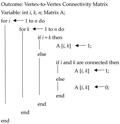
- Any vertex that is adjacent to a monitored edge is observed.
- Any edge connecting two observed vertices is monitored.
- If a vertex is adjacent to a total of edges, and if f these edges are monitored, then all of these edges are observed.
| Algorithm 1: Vertex-to-Vertex Connectivity Matrix |
 |
5. Mathematical Programming Models
- Complete Observability
- Maximum Network Observability
5.1. Constrained Integer Programming with Binary Decision Values
| Algorithm 2: Steps of BBA implementation |
|
|
|
|
|
5.2. Boolean Semi-Definite Programming Model
5.3. Quadratic Constrained Binary Optimization Model
- The iterative process ends up with two explored nodes, as we illustrate in the log files in the Appendix C and Appendix D. This solution is established on the optimization run of two external solvers at the same time [9,10,11].
5.4. Maximizing Programming Models
- An objective function is declared in getting optimized by giving the number of times a power network is observed.
- The observability of every vertex is measured, and the BOI is calculated for every vertex.
- Afterward, the sum of all times by which the power network is monitored is summed, and the SORI is derived.
- An optimal PMU placement set is given as having the maximum SORI.
- i.
- Constrained Integer Programming with Binary Decision Values
- ii.
- Constrained Polynomial Optimization Problem with Binary Decision Variables
- iii.
- Boolean Semi-Definite Programming Model
- The BILP model is written in symbolic format, where the YALMIP BBA solves the problem by invoking a powerful advanced ILP solver to count the upper and lower bounds and solve the linear programming relaxations.
- The Boolean polynomial model is transformed into a polyhedron and solved by the YALMIP BBA function, which constructs a BBA tree where the upper and lower bounds are computed to be equal at the final root node.
- The Boolean SDP model is also written in the same programming language, where the CUTSDP relaxes the second-order conic constraints through a cutting-plane strategy implemented by an ILP function.
- The optimization ends with accuracy because the difference between these bounds delivers a zero-tolerance gap. This tolerance measure means that a global optimal solution is obtained.
- The objective value is considered to be the upper bound for the minimization problem and the lower bound for the maximization problem.
- iv.
- Solving the optimization models with a BBA inside an absolute gap
- Initialization;
- Choose region;
- Lower bound;
- Upper bound;
- Pruning;
- Check region; and
- Branching.
6. Suboptimality Criteria and Convergence Tasks
6.1. Termination Criteria of BBA for Convergence of the Optimization Run [64,65,66,67]
6.2. Convergence Analysis
7. Solution of the Algorithmic Scheme Approaches and Optimization Results
- BBA reduces the computational complexity based on the constraint function; either binary connectivity, LMI constraints, or polynomial constraints are easy to optimize. This can speed up the optimization process related to existing methods for obtaining a global solution point.
- The proposed optimization models are easy to implement in a symbolic format in YALMIP/MATLAB, and BBA makes it easy to optimize those models.
- The time spent on the entire optimization process illustrates that the procedure has low time complexity in achieving optimality.
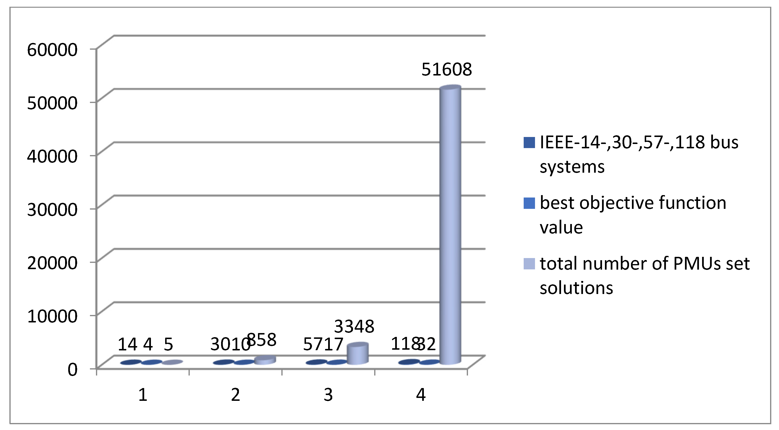
- The proposed models are tested on 14-, 30-, 57, and a medium-size model of the IEEE-118 bus system. This fact enacts the tendency to extend the OPP to larger power systems.
7.1. Results of Complete Observability of the Electricity Power Transmission Grid
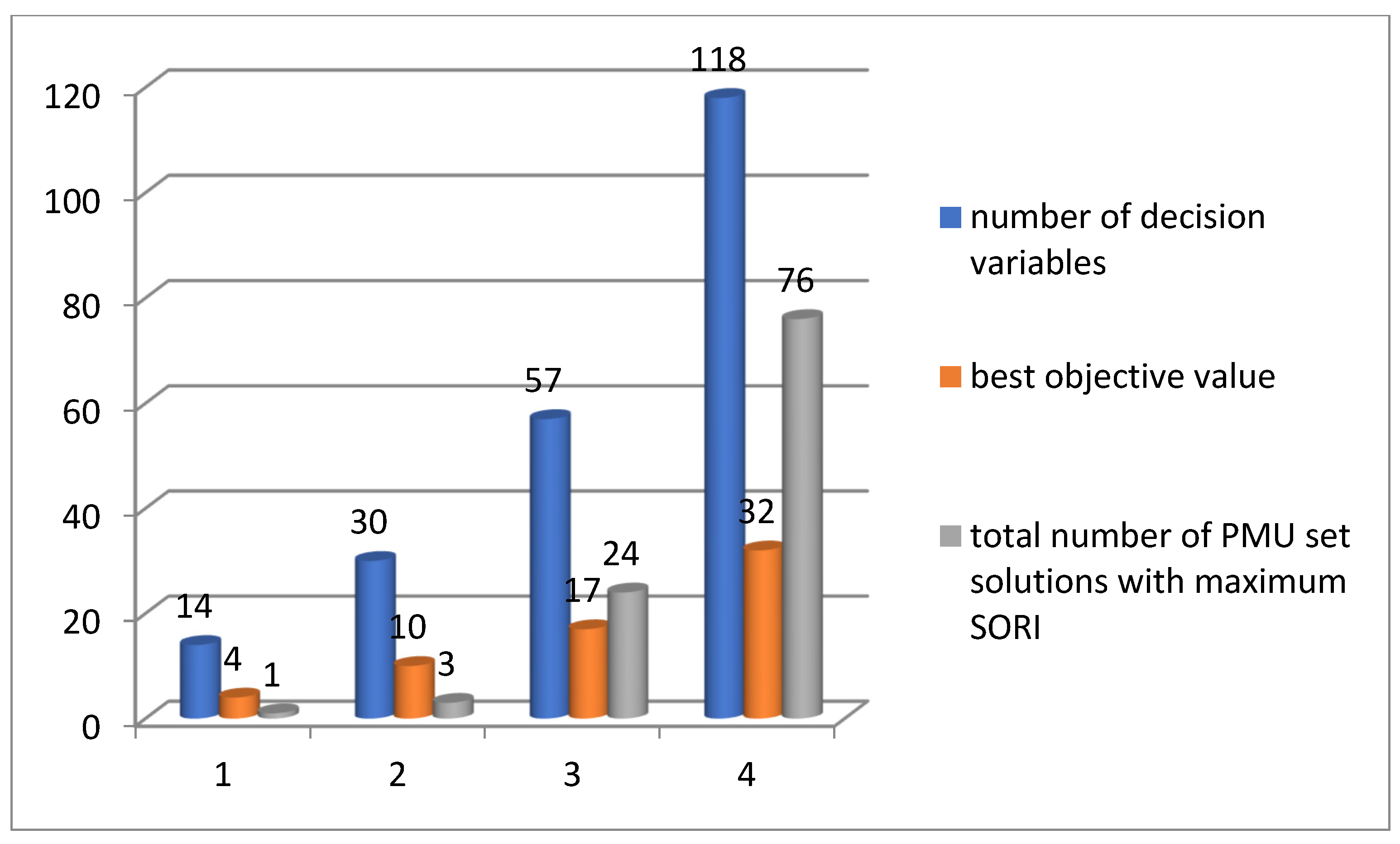
7.2. Results of Maximum Observation of the Electricity Power Transmission Grid
8. Discussion
9. Conclusions
10. Further Research Based on the Topics Studied in This Study
- The future grid will have the capability to incorporate a large number of PMUs to help a lot with utilities and customers’ requirements for constant power supply at the lowest possible cost.
- We propose those PMU arrangements that improve power grid reliability through the maximum observation of the power grid state estimator tool installed in the system operator.
- It produces a complete working OPP solution with accuracy and improved ability to accomplish the aim for the exact number of PMUs under guarantee as well as those solutions satisfying maximum reliability.
- A future direction is to extend our symbolic programming models and computational way of their solutions under any contingencies in SGs.
- Future research could investigate the combination of PMUs with AI and ML algorithms to enable real-time detection and response to cyberattacks.
- It also works as a first test for a novel algorithmic scheme to use a global optimizer routine for solving combinatorial problems with the symbolical programming language and finding a global solution point.
Author Contributions
Funding
Data Availability Statement
Conflicts of Interest
Abbreviations
| SCADA | Supervisory Control and Data Acquisition |
| PMU | Phasor Measuring Unit |
| PDC | Phasor Data Concentrator |
| SG | Smart Grid |
| WAMS | Wide Area Monitoring Systems |
| PDC | Power Dominating Set |
| OPP | Optimal PMU Placement |
| SORI | System Observability Redundancy Index |
| BOI | Bus Observability Index |
| MILP | Mixed-Integer-Linear Program |
| QCBO | Quadratic Constrained Binary Optimization |
| LCBO | Linear Constrained Binary Optimization |
| SCIP | Solve Constraint Integer Program |
| BBA | Branch-and-Bound Algorithm |
| s-BBA | Spatial Branch-and-Bound Algorithm |
| TolGapAbs | Tolerance Gap Absolute |
| MIPGapAb | Mixed-Integer Program Gap Absolute |
Appendix A
Appendix B

| IEEE-Power Systems | PMUs Number | Minimum SORI | Maximum SORI |
|---|---|---|---|
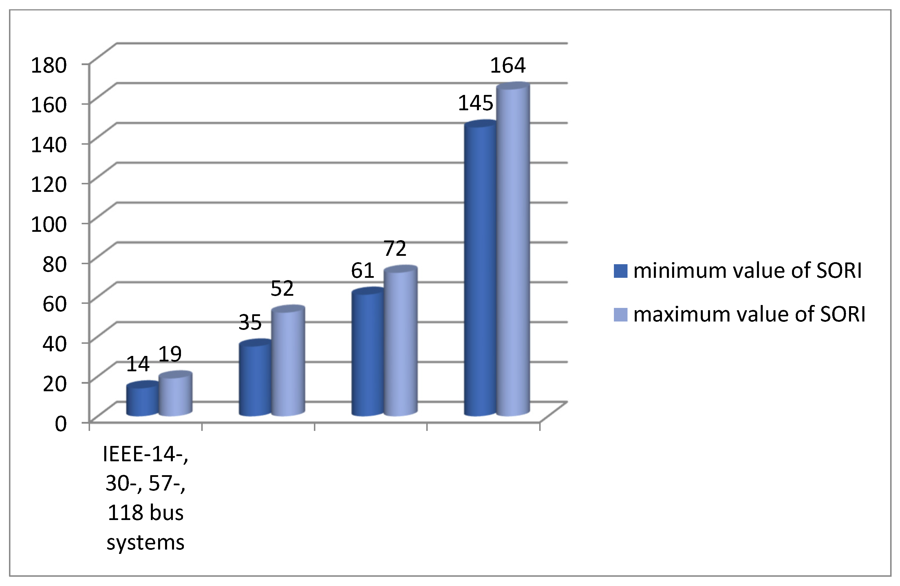
| IEEE-14 bus | 4 | 14 | 19 |
| IEEE-30 bus | 10 | 35 | 52 |
| IEEE-57 bus | 17 | 61 | 72 |
| IEEE-118 bus | 32 | 145 | 164 |
| Mixed-Integer-Linear-ProgramMixed-Integer-Linear-Program Implementation in YALMIP Software. | |||
|---|---|---|---|
| IEEE-Systems | GUROBI | SCIP | Intlinprog |
| Optimal PMU Locations | |||
| 14-bus | 2, 7, 10, 13 | 2, 7, 11, 13 | 2, 8, 10, 13 |
| 30-bus | 1, 5, 6, 9, 10, 12, 15, 19, 25, 27 | 2, 4, 6, 9, 10, 12, 15, 19, 25, 30 | 1, 5, 8, 10, 11, 12, 19, 23, 26, 29 |
| 57-bus | 2, 6, 12, 19, 22, 25, 27, 29, 32, 36, 39, 41, 45, 46, 49, 51, 54 | 2, 6, 12, 14, 19, 22, 25, 27, 32, 36, 39, 41, 44, 47, 50, 52, 55 | 1, 4, 9, 20, 23, 27, 29, 30, 32, 36, 38, 41, 45, 46, 50, 54, 57 |
| 118-bus | 1, 5, 9, 12, 15, 17, 21, 23, 28, 30, 36, 40, 44, 46, 50, 52, 56, 62, 63, 68, 71, 75, 77, 80, 85, 86, 91, 94, 102, 105, 110, 114 | 3, 5, 9, 11, 12, 17, 21, 25, 28, 34, 37, 40, 45, 49, 52, 56, 62, 63, 68, 70, 71, 75, 77, 80, 85 86, 90, 94, 101, 105, 110, 114 | 2, 5, 10, 12, 15, 17, 21, 25, 29, 34, 37, 41, 45, 49, 53, 56, 62, 64, 72, 73, 75, 77, 80, 85, 87, 91, 94, 101, 105, 110, 114, 116 |
| Mixed-Integer-Linear-Program Implementation in YALMIP Software. | |||
|---|---|---|---|
| IEEE-Systems | GUROBI | SCIP | Intlinprog |
| Optimal PMU Locations | |||
| 14-bus | 2, 6, 7, 9 | 2, 6, 7, 9 | 2, 6, 7, 9 |
| 30-bus | 2, 4, 6, 9, 10, 12, 15, 20, 25, 27 | 2, 4, 6, 9, 10, 12, 15, 18, 25, 27 | 2, 4, 6, 9, 10, 12, 15, 19, 25, 27 |
| 57-bus | 1, 4, 6, 9, 15, 20, 24, 25, 28, 32, 36, 38, 41, 46, 51, 53, 57 | 1, 4, 6, 9, 15, 20, 24, 25, 28, 32, 36, 38, 39, 41, 46, 50, 53 | 1, 4, 6, 9, 15, 20, 24, 28, 31, 32, 36, 38, 41, 46, 50, 53, 57 |
| 118-bus | 3, 5, 9, 12, 15, 17, 21, 25, 28, 34, 37, 40, 45, 49, 53, 56, 62, 64, 68, 70, 71, 78, 85, 86, 89, 92, 96, 100, 105, 110, 114, 118 | 3, 5, 9, 12, 15, 17, 21, 25, 28, 34, 37, 40, 45, 49, 52, 56, 62, 64, 68, 70, 71, 76, 78, 85, 86, 89, 92, 96, 100, 105, 110, 114 | 3, 5, 9, 12, 15, 17, 21, 25, 29, 34, 37, 40, 45, 49, 53, 56, 62, 64, 68, 70, 71, 75, 77, 80, 85, 86, 91, 94, 101, 105, 110, 114 |
| Mixed-Integer-Linear-Program Implementation in YALMIP Software. | |||
|---|---|---|---|
| IEEE-Systems | GUROBI | SCIP | Intlinprog |
| Optimal PMU Locations | |||
| 14-bus | 2, 8, 10, 13 | 2, 6, 8, 9 | 2, 7, 11, 13 |
| 30-bus | 1, 5, 8, 10, 11, 12, 19, 23, 26, 29 | 1, 2, 6, 10, 11, 12, 18, 23, 26, 27 | 3, 5, 8, 10, 11, 12, 15, 20, 25, 30 |
| 57-bus | 1, 4, 9, 20, 24, 28, 29, 30, 32, 36, 38, 39, 41, 44, 46, 50, 53 | 2, 6, 12, 19, 22, 25, 27, 32, 36, 39, 41, 45, 46, 47, 50, 52, 55 | 3, 6, 12, 15, 19, 22, 25, 26, 29, 32, 36, 38, 41, 46, 50, 54, 57 |
| 118-bus | 3, 5, 10, 12, 15, 17, 21, 23, 28, 30, 36, 40, 43, 45, 49, 52, 56, 62, 64, 71, 75, 77, 80, 85, 87, 91, 94, 101, 105, 110, 114, 116 | 2, 5, 10, 12, 15, 17, 20, 23, 29, 30, 36, 40, 43, 46, 51, 54, 57, 62, 64, 71, 75, 77, 80, 85, 87 91, 94, 102, 105, 110, 115, 116 | 3, 5, 10, 12, 15, 17, 21, 25, 28, 34, 37, 42, 45, 49, 52, 56, 62, 64, 71, 72, 75, 77, 80, 85, 87, 90, 94, 102, 105, 110, 114, 116 |
| Mixed-Integer-Linear-Program Implementation in YALMIP Software. | |||
|---|---|---|---|
| IEEE- Systems | GUROBI | SCIP | Intlinprog |
| Optimal PMU Locations | |||
| 14-bus | 2, 6, 7, 9 | 2, 6, 7, 9 | 2, 6, 7, 9 |
| 30-bus | 2, 4, 6, 9, 10, 12, 15, 20, 25, 27 | 2, 4, 6, 9, 10, 12, 15, 18, 25, 27 | 2, 4, 6, 9, 10, 12, 15, 19, 25, 27 |
| 57-bus | 1, 4, 6, 9, 15, 20, 24, 28, 31, 32, 36, 38, 39, 41, 47, 51, 53 | 1, 4, 6, 9, 15, 20, 24, 25, 28, 32, 36, 38, 41 46, 50, 53, 57 | 1, 4, 6, 9, 15, 20, 24, 28, 31, 32, 36, 38, 41, 46, 51, 53, 57 |
| 118-bus | 3, 5, 9, 12, 15, 17, 21, 25, 29, 34, 37, 40, 45, 49, 52, 56, 62, 64, 68, 70, 71, 78, 85, 86, 89, 92, 96, 100, 105, 110, 114, 118 | 3, 5, 9, 12, 15, 17, 21, 25, 29, 34, 37, 40, 45, 49, 52, 56, 62, 64, 68, 70, 71, 75, 77, 80, 85 86, 90, 94, 102, 105, 110, 114 | 3, 5, 9, 12, 15, 17, 21, 25, 28, 34, 37, 40, 45, 49, 52, 56, 62, 64, 68, 70, 71, 78, 85, 86, 89, 92, 96, 100, 105, 110, 114, 118 |
| IEEE-Systems | MOSEK | SCIP |
|---|---|---|
| 14-bus | 2, 6, 7, 9 | 2, 7, 10, 13 |
| 30-bus | 1, 2, 6, 9, 10, 12, 15, 18, 25, 27 | 1, 2, 6, 9, 10, 12, 15, 19, 25 30 |
| 57-bus | 1, 6, 13, 15, 19, 22, 25, 26, 29, 32, 36, 38, 41, 46, 51, 54, 57 | 2, 6, 12, 14, 19, 22, 25, 27, 32 36, 39 41, 44, 47, 50, 52, 55 |
| 118-bus | 1, 6, 9, 11, 12, 17, 21, 25, 29, 34, 37, 41, 45, 49, 53, 56 62, 63, 68, 71, 72, 75, 77, 80 85, 86, 90, 94, 102, 105 110, 114 | 3, 5, 9, 11, 12, 17, 21, 25, 28, 34, 37 40, 45, 49, 52, 56, 62, 63, 68, 70, 71 75, 77, 80, 85, 86 90, 94, 101, 105, 110, 114 |
| IEEE-Systems | MOSEK | SCIP |
|---|---|---|
| 14-bus | 2, 6, 7, 9 | 2, 6, 7, 9 |
| 30-bus | 2, 4, 6, 9, 10, 12, 15, 19, 25, 27 | 2, 4, 6, 9, 10, 12, 15, 20, 25, 27 |
| 57-bus | 1, 4, 6, 9, 15, 20, 24, 25, 28, 32, 36, 38, 41, 46 50, 53, 57 | 1, 4, 6, 9, 15, 24, 25, 28, 32, 36 38, 41 46, 51, 53, 57 |
| 118-bus | 3, 5, 9, 12, 15, 17, 20, 23, 28, 30, 34, 37, 40, 45, 49, 52, 56, 62, 64, 68, 71, 75, 77, 80 85, 86, 90, 94, 102, 105, 110, 114 | 3, 5, 9, 12, 15, 17, 21, 25, 29, 34 37, 40 45, 49, 53, 56, 62, 64, 68, 70, 71, 75, 77, 80, 85, 86, 90, 94 101, 105 110, 114 |
| IEEE-Systems | Intlinprog | Gurobi |
|---|---|---|
| 14-bus | 2, 6, 7, 9 | 2, 6, 7, 9 |
| 30-bus | 1, 5, 8, 10, 11, 12, 19, 23, 26, 29 | 1, 5, 6, 9, 10, 12, 15, 19, 25, 27 |
| 57-bus | 1, 4, 9, 20, 23, 27, 29, 30, 32, 36, 38, 41, 45, 46, 50, 54, 57 | 2, 6, 12, 19, 22, 25, 27, 29, 32, 36, 39, 41, 45, 46, 49, 51, 54 |
| 118-bus | 2, 5, 10, 12, 15, 17, 21, 25, 29, 34, 37, 41, 45, 49, 53, 56, 62, 64, 72, 73, 75, 77, 80, 85, 87, 91, 94, 101, 105, 110, 114, 116 | 1, 5, 9, 12, 15, 17, 21, 23, 28, 30, 36, 40, 44, 46, 50, 52, 56, 62, 63, 68, 71, 75, 77, 80, 85, 86, 91, 94, 102, 105, 110, 114 |
| IEEE-Systems | Intlinprog | Gurobi |
|---|---|---|
| 14-bus | 2, 6, 7, 9 | 2, 6, 7, 9 |
| 30-bus | 1, 7, 8, 10, 11, 12, 19, 23, 25, 29 | 1, 5, 6, 9, 10, 12, 15, 19, 25, 27 |
| 57-bus | 1, 4, 7, 9, 20, 22, 25, 27, 32, 36, 39, 41, 44, 46 49, 50, 53 | 2, 6, 12, 19, 22, 25, 27, 29, 32, 36, 39, 41, 45, 46, 49, 51, 54 |
| 118-bus | 1, 6, 9, 11, 12, 17, 21, 25, 28, 34, 37, 4,1 45, 49 52, 56, 62, 63, 68, 70, 71, 78, 85, 86, 91, 92, 96 100, 105, 110, 114, 118 | 1, 5, 9, 12, 15, 17, 21, 23, 25, 28, 34, 37, 40, 45, 49, 52, 56, 62, 63, 68, 71, 75, 77, 80, 85, 86, 91, 94, 102, 105, 110, 114 |
| IEEE-Systems | Intlinprog | Gurobi |
|---|---|---|
| 14-bus | 2, 6, 7, 9 | 2, 6, 7, 9 |
| 30-bus | 2, 4, 6, 9, 10, 12, 15, 19, 25, 27 | 2, 4, 6, 9, 10, 12, 15, 19, 25, 27 |
| 57-bus | 1, 4, 6, 9, 15, 20, 24, 28, 31, 32 36, 38, 41, 46, 50, 53, 57 | 1, 4, 6, 9, 15, 20, 24, 25, 28, 32, 36, 38 41, 46, 51, 53, 57 |
| 118-bus | 3, 5, 9 12, 15, 17, 21, 25, 29, 34 37, 40, 45, 49, 53, 56, 62, 64, 68 70, 71, 75, 77, 80, 85, 86, 91, 94 101, 105, 110, 114 | 3, 5, 9, 12, 15, 17, 21, 25, 29, 34, 37, 40, 45, 49, 53, 56, 62, 64, 68, 70, 71, 75, 77, 80, 85, 86, 90, 94, 101, 105, 110, 114 |
| IEEE-Systems | Intlinprog | Gurobi |
|---|---|---|
| 14-bus | 2, 6, 7, 9 | 2, 6, 7, 9 |
| 30-bus | 2, 4, 6, 9, 10, 12, 15, 20, 25, 27 | 2, 4, 6, 9, 10, 12, 15, 20, 25, 27 |
| 57-bus | 1, 4, 6, 9, 15, 20, 24, 28, 31, 32, 36, 38, 41, 47 50, 53, 57 | 1, 4, 6, 9, 15, 20, 24, 25, 28, 32, 36, 38, 41, 47, 51, 53, 57 |
| 118-bus | 3, 5, 9, 12, 15, 17, 20, 23, 29, 30, 34, 37, 40, 45, 49, 52, 56, 62, 64, 68, 71, 75, 77, 80, 85, 86, 91, 94, 102, 105, 110, 115 | 3, 5, 9, 12,15, 17, 20, 23, 28, 30, 34, 37, 40, 45, 49, 53, 56, 62, 64, 68, 71, 75, 77, 80, 85, 86, 90, 94, 102, 105, 110, 115 |
Appendix C
- I.
- Mixed-Integer Linear Programming Model
| + Solver chosen: BMIBNB |
| + Processing objective function |
| + Processing constraints |
| + Branch and bound started |
| * Starting YALMIP global branch and bound. |
| * Upper solver: GUROBI |
| * Lower solver: GUROBI |
| * LP solver: GUROBI |
| * -Extracting bounds from model |
| * -Performing root-node bound propagation |
| * -Calling upper solver + Calling GUROBI |
| (found a solution!) |
| * -Branch-variables: 0 |
| * -More root-node bound-propagation |
| * -Performing LP-based bound-propagation |
| * -And some more root-node bound-propagation |
| * Starting the B and B process |
| Node Upper Gap(%) Lower Open Time |
| + Calling GUROBI |
| 1: 1.00000E+01 0.00 1.00000E+01 0 0s Poor lower bound |
| * Finished. Cost: 10 (lower bound: 10, relative gap 0%) |
| * Termination with all nodes pruned |
| * Timing: 17% spent in upper solver (1 problems solved) |
| * 1% spent in lower solver (1 problems solved) |
| * 1% spent in LP-based domain reduction (0 problems solved) |
| * 1% spent in upper heuristics (0 candidates tried) |
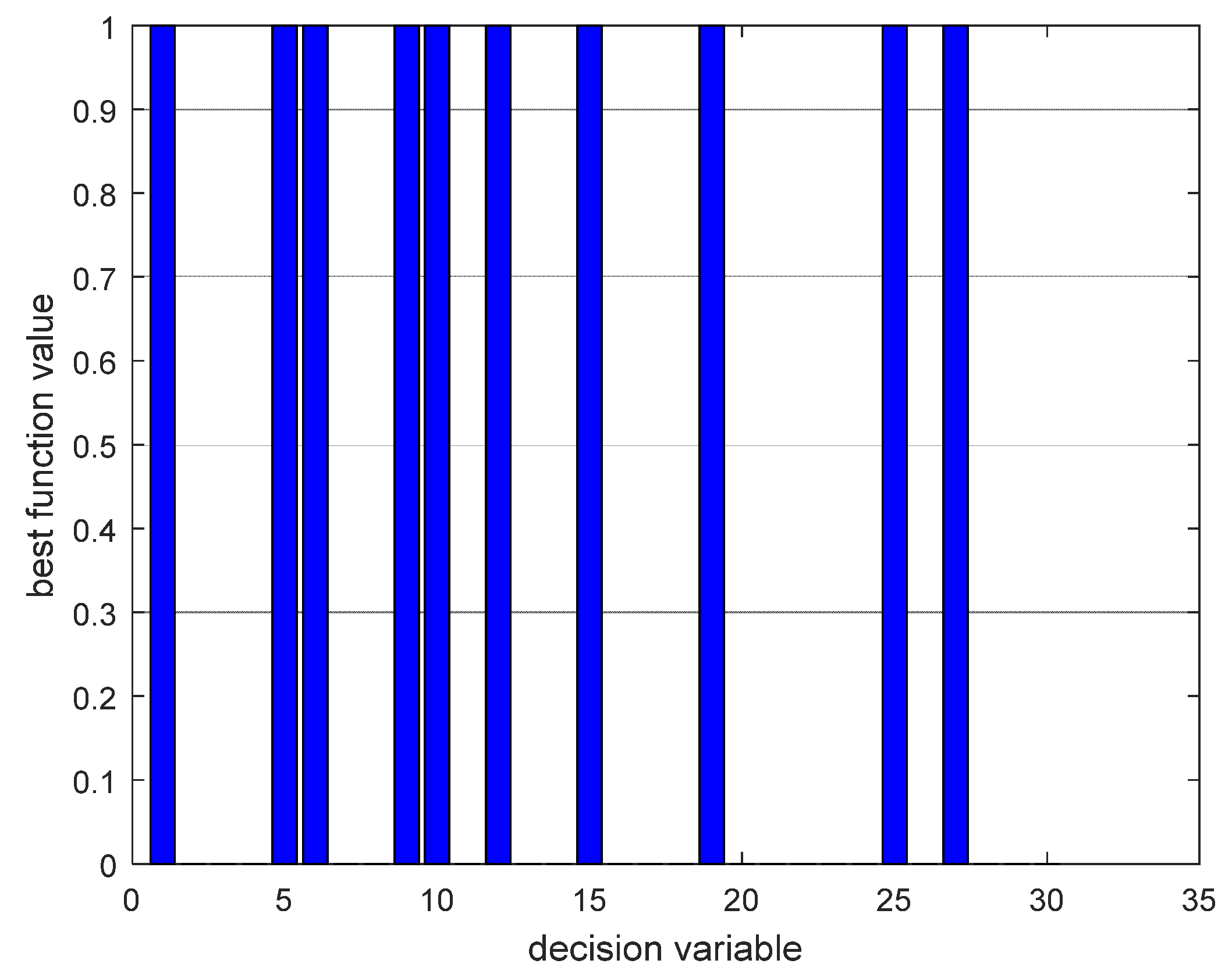
| Optimal PMU Placement Sites |
|---|
| 1, 5, 6, 9, 10, 12, 15, 19, 25, 27 |
| Optimal number of PMUs: 10 |
| SORI: 48 |
| best function value: 10 |

- II.
- Quadratic Constrained Binary Optimization Model
| + Solver chosen: BMIBNB |
| + Processing objective function |
| + Processing constraints |
| + Branch and bound started |
| * Starting YALMIP global branch and bound. |
| | #3| Equality constraint (polynomial) 1 × 1| 1 to 1| |
| | #4| Equality constraint (polynomial) 1 × 1| 1 to 1| |
| | #5| Equality constraint (polynomial) 1 × 1| 1 to 1| |
| | #6| Equality constraint (polynomial) 1 × 1| 1 to 1| |
| | #7| Equality constraint (polynomial) 1 × 1| 1 to 1| |
| | #8| Equality constraint (polynomial) 1 × 1| 1 to 1| |
| | #9| Equality constraint (polynomial) 1 × 1| 1 to 1| |
| | #10| Equality constraint (polynomial) 1 × 1| 1 to 1| |
| | #11| Equality constraint (bilinear) 1 × 1 | 1 to 1| |
| | #12| Equality constraint (polynomial) 1 × 1| 1 to 1| |
| | #13| Equality constraint (bilinear) 1 × 1| 1 to 1| |
| | #14| Equality constraint (polynomial) 1 × 1| 1 to 1| |
| | #15| Equality constraint (polynomial) 1 × 1| 1 to 1| |
| | #16| Equality constraint (polynomial) 1 × 1| 1 to 1| |
| | #17| Equality constraint (polynomial) 1 × 1| 1 to 1| |
| | #18| Equality constraint (polynomial) 1 × 1| 1 to 1| |
| | #19| Equality constraint (polynomial) 1 × 1| 1 to 1| |
| | #20| Equality constraint (polynomial) 1 × 1| 1 to 1| |
| | #21| Equality constraint (polynomial) 1 × 1| 1 to 1| |
| | #22| Equality constraint (polynomial) 1 × 1| 1 to 1| |
| | #23| Equality constraint (polynomial) 1 × 1| 1 to 1| |
| | #24| Equality constraint (polynomial) 1 × 1| 1 to 1| |
| | #25| Equality constraint (polynomial) 1 × 1| 1 to 1| |
| | #26| Equality constraint (bilinear) 1 × 1 | 1 to 1| |
| | #27| Equality constraint (polynomial) 1 × 1| 1 to 1| |
| | #28| Equality constraint (polynomial) 1 × 1| 1 to 1| |
| | #29| Equality constraint (polynomial) 1 × 1| 1 to 1| |
| | #30| Equality constraint (polynomial) 1 × 1| 1 to 1| |
| | #31| Binary constraint| | |
| +++++++++++++++++++++++++++++++++++++++++++++++++++++++++++++++++++++ |
| * Starting YALMIP global branch and bound. |
| * Upper solver: fmincon |
| * Lower solver: GUROBI |
| * LP solver: GUROBI |
| * -Extracting bounds from model |
| * -Performing root-node bound propagation |
| * -- Calling upper solver + Calling FMINCON (no solution found) |
| * -Branch-variables: 175 |
| * -More root-node bound-propagation |
| * -Performing LP-based bound-propagation |
| * -And some more root-node bound-propagation |
| * Starting the B AND B process |
| Node Upper Gap(%) Lower Open Time |
| + Calling GUROBI |
| + Calling GUROBI |
| + Calling FMINCON |
| 1: 1.00000E+01 0.00 1.00000E+01 2 4 s Solution found by heuristics |
| + Calling GUROBI |
| 2: 1.00000E+01 0.00 1.00000E+01 0 4 s Poor lower bound | Pruned stack based on new upper bound |
| * Finished. Cost: 10 (lower bound: 10, relative gap 0%) |
| * Termination with all nodes pruned |
| * Timing: 9% spent in upper solver (2 problems solved) |
| * 9% spent in lower solver (2 problems solved) |
| * 51% spent in LP-based domain reduction (350 problems solved) |
| * 1% spent in upper heuristics (1 candidates tried) |
| Quadratic scalar (real, homogeneous, 30 variables) |
| Current value: 10 |
| Coefficients range: 1 to 1 |
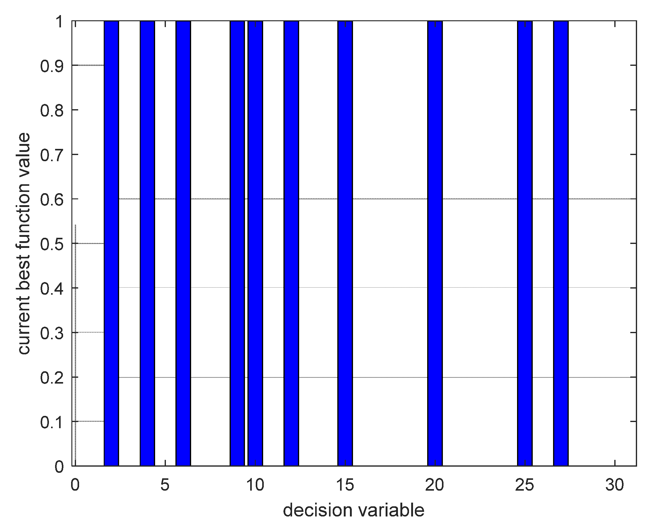
| Optimal PMU Placement Sites |
|---|
| 1, 5, 8, 10, 11, 12, 19, 23, 26, 29 |
| Optimal number of PMUs: 10 |
| SORI: 35 |
| best function value: 10 |
- III.
- Semi-Definite Programming Model
| +++++++++++++++++++++++++++++++++++++++++++++++++++++++++++++++++ |
| | ID| Constraint| Coefficient range| |
| +++++++++++++++++++++++++++++++++++++++++++++++++++++++++++++++++ |
| | #1| Matrix inequality (integer) 30 × 30| 0.009 to 8| |
| | #2| Binary constraint (integer)| | |
| +++++++++++++++++++++++++++++++++++++++++++++++++++++++++++++++++ |
|
+ Solver chosen: CUTSDP + Processing objective function + Processing constraints + Cutting plane solver started* Starting YALMIP cutting plane for MISDP based on MILP |
| * Lower solver: GUROBI |
| * Max iterations: Inf |
| * Max time: 3600 |
| Node Phase Cone infeas Integrality infeas Lower bound Upper bound LP cuts Elapsed time |
| 1: Continuous 0.000E+00 0.000E+00 1.000E+01 Inf 29 0.1 |
| 2: Integer 0.000E+00 0.000E+00 1.000E+01 1.000E+01 30 0.1 |
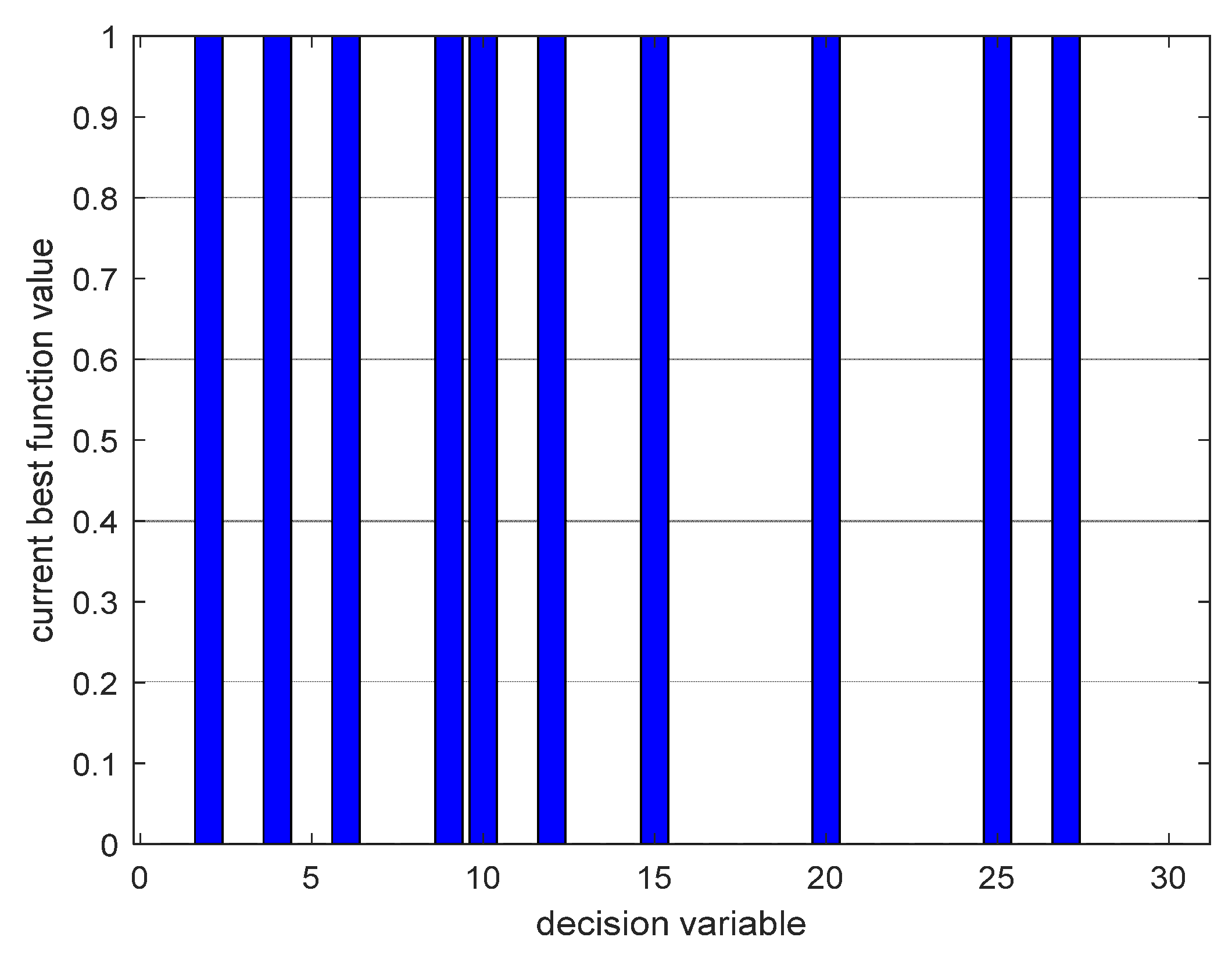
| Optimal number of PMUs: 10 |
| SORI: 48 |
| best function value: 10 |
| Optimal PMU Positioning Sites |
|---|
| 1, 5, 6, 9, 10, 12, 15, 19, 25, 27 |

Appendix D
- Aim to maximize the redundancy of synchronized measurements in power system observability
- I.
- Mixed-Integer Linear Programming Model
| + Solver chosen: BMIBNB |
| + Processing objective function |
| + Processing constraints |
| + Branch and bound started |
| * Starting YALMIP global branch and bound. |
| * -Performing root-node bound propagation |
| -Calling upper solver + Calling GUROBI (found a solution!) |
| * -Branch-variables: 0 |
| * -More root-node bound-propagation |
| * -Performing LP-based bound-propagation |
| * -And some more root-node bound-propagation |
| * Starting the B and B process |
| Node Upper Gap(%) Lower Open Time |
| 1: −1.73333E+00 0.00 −1.73333E+00 0 0 s Poor lower bound |
| * Finished. Cost: −1.7333 (lower bound: −1.7333, relative gap 0%) |
| * Termination with all nodes pruned |
| * Timing: 14% spent in upper solver (1 problems solved) |
| * 7% spent in lower solver (1 problems solved) |
| * 1% spent in LP-based domain reduction (0 problems solved) |
| * 1% spent in upper heuristics (0 candidates tried) |
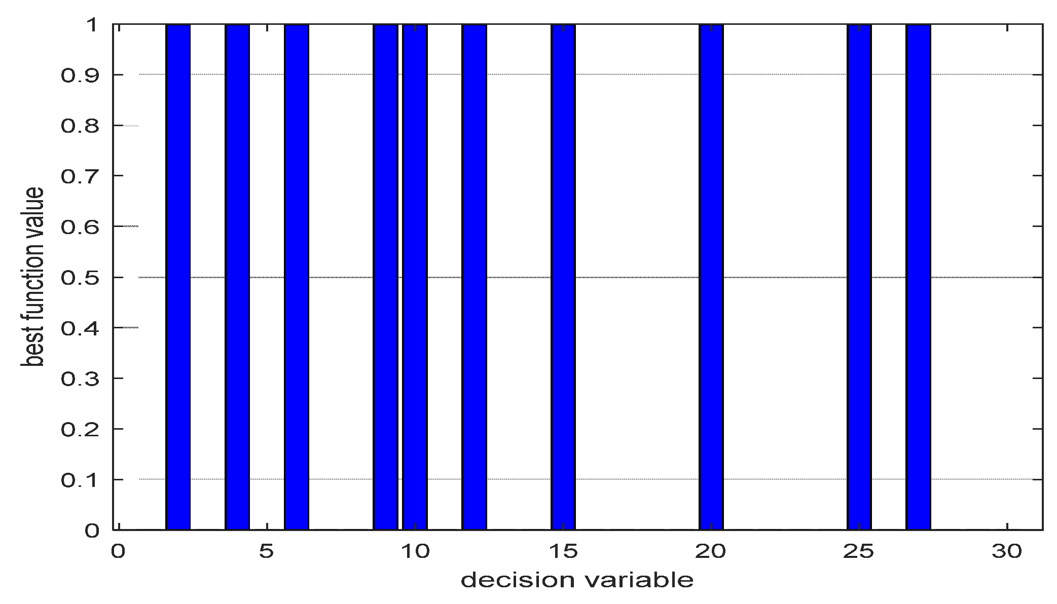
| ans = |
| Optimal PMU locations |
| 2 4 6 9 10 12 15 20 25 27 |
| Optimal number of PMUs: 10 |
| SORI: 52 |
| obj: −1.733333e+00 |

- II.
- Linear Constrained Binary Optimization Model
| + Solver chosen: BMIBNB |
| + Processing objective function |
| + Processing constraints |
| + Branch and bound started |
| * Starting YALMIP global branch and bound. |
| | #3| Equality constraint (polynomial) 1 × 1| 1 to 1| |
| | #4| Equality constraint (polynomial) 1 × 1| 1 to 1| |
| | #5| Equality constraint (polynomial) 1 × 1| 1 to 1| |
| | #6| Equality constraint (polynomial) 1 × 1| 1 to 1| |
| | #7| Equality constraint (polynomial) 1 × 1| 1 to 1| |
| | #8| Equality constraint (polynomial) 1 × 1| 1 to 1| |
| | #9| Equality constraint (polynomial) 1 × 1| 1 to 1| |
| | #10| Equality constraint (polynomial) 1 × 1| 1 to 1| |
| | #11| Equality constraint (bilinear) 1 × 1| 1 to 1| |
| | #12| Equality constraint (polynomial) 1 × 1| 1 to 1| |
| | #13| Equality constraint (bilinear) 1 × 1| 1 to 1| |
| | #14| Equality constraint (polynomial) 1 × 1| 1 to 1| |
| | #15| Equality constraint (polynomial) 1 × 1| 1 to 1| |
| | #16| Equality constraint (polynomial) 1 × 1| 1 to 1| |
| | #17| Equality constraint (polynomial) 1 × 1| 1 to 1| |
| | #18| Equality constraint (polynomial) 1 × 1| 1 to 1| |
| | #19| Equality constraint (polynomial) 1 × 1| 1 to 1| |
| | #20| Equality constraint (polynomial) 1 × 1| 1 to 1| |
| | #21| Equality constraint (polynomial) 1 × 1| 1 to 1| |
| | #22| Equality constraint (polynomial) 1 × 1| 1 to 1| |
| | #23| Equality constraint (polynomial) 1 × 1| 1 to 1| |
| | #24| Equality constraint (polynomial) 1 × 1| 1 to 1| |
| | #25| Equality constraint (polynomial) 1 × 1| 1 to 1| |
| | #26| Equality constraint (bilinear) 1 × 1 | 1 to 1| |
| | #27| Equality constraint (polynomial) 1 × 1| 1 to 1| |
| | #28| Equality constraint (polynomial) 1 × 1| 1 to 1| |
| | #29| Equality constraint (polynomial) 1 × 1| 1 to 1| |
| | #30| Equality constraint (polynomial) 1 × 1| 1 to 1| |
| | #31| Equality constraint 1 × 1| 1 to 10| |
| +++++++++++++++++++++++++++++++++++++++++++++++++++++++++++++++++++++ |
| * Starting YALMIP global branch and bound. |
| * Upper solver: fmincon |
| * Lower solver: GUROBI |
| * LP solver: GUROBI |
| * -Extracting bounds from model |
| * -Perfoming root-node bound propagation |
| * -Calling upper solver + Calling FMINCON (no solution found) |
| * -Branch-variables: 30 |
| * -More root-node bound-propagation |
| * -Performing LP-based bound-propagation |
| * -And some more root-node bound-propagation |
| * Starting the B and B process |
| Node Upper Gap(%) Lower Open Time |
| + Calling GUROBI |
| + Calling FMINCON |
| 1: −1.73333E+00 0.00 −1.73333E+00 2 2 s Solution found by heuristics |
| + Calling GUROBI |
| 2: −1.73333E+00 0.00 −1.73333E+00 0 3 s Poor lower bound | Pruned stack based on new upper bound |
| * Finished. Cost: −1.7333 (lower bound: −1.7333, relative gap 0%) |
| * Termination with all nodes pruned |
| * Timing: 10% spent in upper solver (2 problems solved) |
| * 6% spent in lower solver (2 problems solved) |
| * 19% spent in LP-based domain reduction (60 problems solved) |
| * 1% spent in upper heuristics (1 candidates tried) |
| Optimal PMU locations |
| 2 4 6 9 10 12 15 20 25 27 |
| Linear scalar (real, binary, 30 variables) |
| Current value: −1.7333 |
| Coefficients range: 0.066667 to 0.26667 |
| SORI = |
| 52 |
| ans = |
| ‘bmibnb’ |

- III.
- Semi Definite Programming
| + Solver chosen: CUTSDP + Processing objective function + Processing constraints + Cutting plane solver started* Starting YALMIP cutting plane for MISDP based on MILP |
| * Lower solver: GUROBI |
| * Max iterations: Inf |
| * Max time: 3600 |
| Node Phase Cone infeas Integrality infeas Lower bound Upper bound LP cuts Elapsed time |
| 1: Continuous 0.000E+00 0.000E+00 −1.733E+00 Inf 29 0.1 |
| 2: Integer 0.000E+00 0.000E+00 −1.733E+00 −1.733E+00 29 0.1 |
| SORI = |
| 52 |
| ans = |
| ‘ CUTSDP ‘ |
| PMU Positioning Sites |
|---|
| 2, 4, 6, 9, 10, 12, 15, 20, 25, 27 |

Appendix E
| Gurobi Optimizer version 10.0.0 build v10.0.0rc2 (win64) |
| Optimize a model with 57 rows, 57 columns and 213 nonzeros |
| Variable types: 0 continuous, 57 integer (57 binary) |
| Found heuristic solution: objective 20.0000000 |
| Presolve removed 6 rows and 0 columns |
| Presolve time: 0.00 s |
| Presolved: 51 rows, 57 columns, 184 nonzeros |
| Variable types: 0 continuous, 57 integer (57 binary) |
| Root relaxation presolved: 51 rows, 57 columns, 184 nonzeros |
| Root relaxation: objective 1.600000e+01, 69 iterations, 0.01 s (0.00 work units) |
| Nodes | Current Node | Objective Bounds | Work |
| Expl Unexpl | Obj Depth IntInf | Incumbent BestBd Gap | It/Node Time |
| 0 0 16.00000 0 20 20.00000 16.00000 20.0% - 0 s |
| H 0 0 19.0000000 16.00000 15.8% - 0 s |
| H 0 0 17.0000000 16.00000 5.88% - 0 s |
| 0 0 16.50000 0 13 17.00000 16.50000 2.94% - 0 s |
| Optimal solution found at node 0 - now completing solution pool… |
| Nodes | Current Node | Pool Obj. Bounds | Work |
| | | Worst | |
| Expl Unexpl | Obj Depth IntInf | Incumbent BestBd Gap | It/Node Time |
| 0 0 16.50000 0 17 - 16.50000 - - 0 s |
| 0 0 - 0 - 17.00000 - - 0 s |
| 0 0 - 0 - 17.00000 - - 0 s |
| 0 0 - 0 - 17.00000 - - 0 s |
| 0 2 - 0 - 17.00000 - - 0 s |
| Cutting planes: |
| Gomory: 1 |
| Zero half: 4 |
| Explored 78447 nodes (95209 simplex iterations) in 3.25 s (0.55 work units) |
| Thread count was four (of four available processors) |
| Solution count 3348: 17 17 17 … 17 |
| Optimal solution found (tolerance 1.00e−04) |
| Best objective 1.700000000000e+01, best bound 1.700000000000e+01, gap 0.0000% |
| Elapsed time is 3.317972 s. |
| Optimal objective: 1.700000e+01 |
| PMU Placement Set |
|---|
| 1, 4, 7, 10, 20, 23, 25, 26, 29, 32, 36, 39, 41, 44, 46, 49, 54 |

| PMU Placement Locations under Complete Observability Scenario | SORI |
|---|---|
| 1, 4, 7, 10, 20, 23, 25, 26, 29, 32, 36, 39, 41, 44, 46, 49, 54 | 64 |
| 2, 6, 12, 19, 22, 25, 27, 32, 36, 38, 41, 45, 46, 50, 52, 55, 57 | 64 |
| 1, 4, 7, 9, 20, 22, 25, 27, 32, 36, 38, 41, 45, 46, 50, 53, 57 | 68 |
| 1, 6, 7, 9, 15, 19, 22, 25, 27, 32, 36, 38, 41, 47, 50, 53, 57 | 71 |
| 1, 6, 9, 15, 19, 22, 25, 27, 32, 36, 38, 41, 47, 50, 52, 55, 57 | 70 |
| 2, 6, 12, 15, 19, 22, 25, 27, 32, 36, 38, 41, 47, 50, 52, 55, 57 | 67 |
| 2, 6, 12, 19, 22, 25, 26, 29, 32, 36, 38, 41, 45, 46, 50, 54, 57 | 65 |
| 2, 6, 12, 19, 22, 25, 27, 29, 32, 36, 38, 41, 45, 46, 50, 54, 57 | 65 |
| 2, 6, 12, 19, 22, 25, 27, 29, 32, 36, 41, 45, 46, 49, 50, 54, 57 | 64 |
| 2, 6, 12, 19, 22, 25, 27, 29, 32, 36, 38, 41, 45, 46, 51, 54, 57 | 65 |
| 2, 6, 12, 19, 22, 25, 27, 29, 32, 36, 38, 39, 41, 45, 46, 50, 54 | 65 |
| 2, 6, 12, 19, 22, 25, 27, 32, 36, 38, 41, 45, 46, 51, 52, 55, 57 | 64 |
| 2, 6, 12, 19, 22, 25, 27, 32, 36, 38, 39, 41, 45, 46, 50, 52, 55 | 64 |
| 2, 6, 12, 19, 22, 25, 27, 32, 36, 41, 45, 46, 49, 50, 52, 55, 57 | 63 |
| 1, 4, 6, 9, 15, 20, 24, 25, 28, 32, 36, 38, 41, 46, 50, 53, 57 | 72 |
| 1, 5, 7, 9, 15, 19, 22, 25, 27, 32, 36, 38, 41, 47, 50, 53, 57 | 69 |
| 2, 6, 12, 19, 22, 25, 26, 29, 32, 36, 41, 45, 46, 49, 50, 54, 57 | 64 |
| 2, 6, 12, 19, 22, 25, 27, 32, 36, 38, 39, 41, 45, 46, 51, 52, 54 | 64 |
| 2, 6, 12, 19, 22, 25, 26, 29, 32, 36, 38, 41, 45, 46, 51, 54, 57 | 65 |
| 2, 6, 12, 19, 22, 26, 29, 30, 32, 36, 38, 41, 45, 46, 51, 54, 57 | 65 |
| ++++++++++++++++++++++++++++++++++++++++++++++++++++++++++++ |
| | ID| Constraint| Coefficient range| |
| ++++++++++++++++++++++++++++++++++++++++++++++++++++++++++++ |
| | #1| Element-wise inequality 57 × 1| 1 to 1| |
| | #2| Equality constraint 1 × 1| 1 to 17| |
| ++++++++++++++++++++++++++++++++++++++++++++++++++++++++++++ |
| Set parameter PoolSolutions to value 24 |
| Set parameter PoolSearchMode to value 2 |
| Optimize a model with 58 rows, 57 columns and 270 nonzeros |
| Variable types: 0 continuous, 57 integer (57 binary) |
| Presolve removed 6 rows and 0 columns |
| Presolve time: 0.00 s |
| Presolved: 52 rows, 57 columns, 241 nonzeros |
| Root relaxation: objective −1.271930e+00, 38 iterations, 0.00 s (0.00 work units) |
| Nodes | Current Node | Objective Bounds | Work |
| Expl Unexpl | Obj Depth IntInf | Incumbent BestBd Gap | It/Node Time |
| 0 0 −1.27193 0 10 - −1.27193 - - 0 s |
| H 0 0 −1.1929825 −1.27193 6.62% - 0 s |
| H 0 0 −1.2456140 −1.27193 2.11% - 0 s |
| H 0 0 −1.2631579 −1.27193 0.69% - 0 s |
| 0 0 - 0 −1.26316 −1.26316 0.00% - 0 s |
| Optimal solution found at node 0 - now completing solution pool... |
| Nodes | Current Node | Pool Obj. Bounds | Work |
| | | Worst | |
| Expl Unexpl | Obj Depth IntInf | Incumbent BestBd Gap | It/Node Time |
| 0 0 - 0 - −1.26316 - - 0 s |
| 0 0 - 0 - −1.26316 - - 0 s |
| 0 2 - 0 - −1.26316 - - 0 s |
| Cutting planes: |
| Zero half: 1 |
| Explored 299 nodes (279 simplex iterations) in 0.18 s (0.00 work units) |
| Solution count 24: −1.26316 −1.26316 −1.26316 … −1.26316 |
| No other solutions better than −1.26316 |
| Optimal solution found (tolerance 1.00e−04) |
| Best objective −1.263157894737e+00, best bound −1.263157894737e+00, gap 0.0000% |
| PMU Placement Locations under Maximum Observability Index |
|---|
| 1, 4, 6, 9, 15, 20, 24, 28, 30, 32, 36, 38, 41, 46, 51, 53, 57 |
| 1, 4, 6, 9, 15, 20, 24, 28, 30, 32, 36, 38, 41, 46, 50, 53, 57 |
| 1, 4, 6, 9, 15, 20, 24, 28, 30, 32, 36, 38, 39, 41, 46, 51, 53 |
| 1, 4, 6, 9, 15, 20, 24, 28, 30, 32, 36, 38, 39, 41, 46, 50, 53 |
| 1, 4, 6, 9, 15, 20, 24, 25, 28, 32, 36, 38, 41, 46, 51, 53, 57 |
| 1, 4, 6, 9, 15, 20, 24, 28, 31, 32, 36, 38, 41, 46, 51, 53, 57 |
| 1, 4, 6, 9, 15, 20, 24, 28, 31, 32, 36, 38, 41, 47, 51, 53, 57 |
| 1, 4, 6, 9, 15, 20, 24, 28, 30, 32, 36, 38, 41, 47, 51, 53, 57 |
| 1, 4, 6, 9, 15, 20, 24, 25, 28, 32, 36, 38, 41, 47, 51, 53, 57 |
| 1, 4, 6, 9, 15, 20, 24, 25, 28, 32, 36, 38, 41, 47, 50, 53, 57 |
| 1, 4, 6, 9, 15, 20, 24, 25, 28, 32, 36, 38, 41, 46, 50, 53, 57 |
| 1, 4, 6, 9, 15, 20, 24, 28, 30, 32, 36, 38, 41, 47, 50, 53, 57 |
| 1, 4, 6, 9, 15, 20, 24, 28, 30, 32, 36, 38, 39, 41, 47, 51, 53 |
| 1, 4, 6, 9, 15, 20, 24, 28, 30, 32, 36, 38, 39, 41, 47, 50, 53 |
| 1, 4, 6, 9, 15, 20, 24, 28, 31, 32, 36, 38, 41, 46, 50, 53, 57 |
| 1, 4, 6, 9, 15, 20, 24, 25, 28, 32, 36, 38, 39, 41, 46, 51, 53 |
| 1, 4, 6, 9, 15, 20, 24, 25, 28, 32, 36, 38, 39, 41, 47, 51, 53 |
| 1, 4, 6, 9, 15, 20, 24, 25, 28, 32, 36, 38, 39, 41, 47, 50, 53 |
| 1, 4, 6, 9, 15, 20, 24, 25, 28, 32, 36, 38, 39, 41, 46, 50, 53 |
| 1, 4, 6, 9, 15, 20, 24, 28, 31, 32, 36, 38, 41, 47, 50, 53, 57 |
| 1, 4, 6, 9, 15, 20, 24, 28, 31, 32, 36, 38, 39, 41, 46, 51, 53 |
| 1, 4, 6, 9, 15, 20, 24, 28, 31, 32, 36, 38, 39, 41, 47, 51, 53 |
| 1, 4, 6, 9, 15, 20, 24, 28, 31, 32, 36, 38, 39, 41, 47, 50, 53 |
| 1, 4, 6, 9, 15, 20, 24, 28, 31, 32, 36, 38, 39, 41, 46, 50, 5 3 |
| best function value: −1.263158e+00 |
| Optimal number of PMUs: 17 |
| SORI: 72 |
References
- Phadke, A.G.; Thorp, J.S. Synchronized Phasor Measurements and Their Applications, 2nd ed.; Springer: New York, NY, USA, 2017. [Google Scholar] [CrossRef]
- Mohamed, E. El-Hawary Advances in Electric Power and Energy: Static State Estimation; John Wiley & Sons: Hoboken, NJ, USA, 2020. [Google Scholar]
- Cyman, J.; Raczek, J. Application of Doubly Connected Dominating Sets to Safe Rectangular Smart Grids. Energies 2022, 15, 2969. [Google Scholar] [CrossRef]
- Brimkov, B.; Mikesell, D.; Smith, L. Connected power domination in graphs. J. Comb. Optim. 2019, 38, 292–315. [Google Scholar] [CrossRef]
- Haynes, T.W.; Hedetniemi, S.M.; Hedetniemi, S.T.; Henning, M.A. Domination in graphs applied to electric power networks. SIAM J. Discret. Math. 2002, 15, 519–529. [Google Scholar] [CrossRef]
- Diestel, R. Graph Theory; Springer: Berlin, Germany, 2017; Volume 173, pp. 59–172. [Google Scholar]
- Narsingh, D. Graph Theory with Applications to Engineering and Computer Science; Prentice-Hall Inc.: Mineola, NY, USA, 1974. [Google Scholar]
- Christofides, N. Graph Theory. An Algorithmic Approach’; Academic Press Inc.: Cambridge, MA, USA, 1975. [Google Scholar]
- Arora, J.S. Introduction to Optimum Design, 4th ed.; Elsevier Inc.: Amsterdam, The Netherlands, 2016. [Google Scholar]
- Williams, H.P. Model Building in Mathematical Programming; John Wiley & Sons: New York, NY, USA, 2013. [Google Scholar]
- Karlof, J. Integer Programming and Practice, 1st ed.; CRC Press Taylor & Francis Group, 6000 Broken Sound Parkway NW, Suite 300: Boca Raton, FL, USA, 2006. [Google Scholar]
- Ahmed, M.M.; Amjad, M.; Qureshi, M.A.; Imran, K.; Haider, Z.M.; Khan, M.O. A Critical Review of State-of-the-Art Optimal PMU Placement Techniques. Energies 2022, 15, 2125. [Google Scholar] [CrossRef]
- Biswal, C.; Sahu, B.K.; Mishra, M.; Rout, P.K. Real-Time Grid Monitoring and Protection: A Comprehensive Survey on the Advantages of Phasor Measurement Units. Energies 2023, 16, 4054. [Google Scholar] [CrossRef]
- Paramo, G.; Bretas, A.; Meyn, S. Research Trends and Applications of PMUs. Energies 2022, 15, 5329. [Google Scholar] [CrossRef]
- Menezes, T.S.; Barra, P.H.A.; Dizioli, F.A.S.; Lacerda, V.A.; Fernandes, R.A.S.; Coury, D.V. A Survey on the Application of Phasor Measurement Units to the Protection of Transmission and Smart Distribution Systems. Electr. Power Compon. Syst. 2023, 1, 1–18. [Google Scholar] [CrossRef]
- Joshi, P.M.; Verma, H.K. Synchrophasor measurement applications and optimal PMU placement: A review. Electr. Power Syst. Res. 2021, 199, 107428. [Google Scholar]
- Mohanta, D.K.; Murthy, C.; Sinha Roy, D. A Brief Review of Phasor Measurement Units as Sensors for Smart Grid. Electr. Power Compon. Syst. 2016, 44, 411–425. [Google Scholar]
- Johnson, T.; Moger, T. A critical review of methods for optimal placement of phasor measurement units. Int. Trans. Electr. Energy Syst. 2020, 31, e12698. [Google Scholar]
- Poirion, P.L.; Toubaline, S.; D’Ambrosio, C.; Liberti, L. The power edge set problem. Networks 2016, 68, 104–120. [Google Scholar] [CrossRef]
- Bei, X.; Yoon, Y.J.; Abur, A. Optimal Placement and Utilization of Phasor Measurements for State Estimation; PSERC Publication: Tempe, AZ, USA, 2005; pp. 1–6. [Google Scholar]
- Xu, B.; Abur, A. Observability Analysis and Measurement Placement for Systems with PMUs. In Proceedings of the IEEE PES Power Systems Conference and Exposition, New York, NY, USA, 10–13 October 2004; pp. 2–5. [Google Scholar]
- Dua, D.; Dambhare, S.; Gajbhiye, R.K.; Soman, S.A. Optimal Multistage Scheduling of PMU Placement: An ILP Approach. IEEE Trans. Power Deliv. 2008, 23, 1812–1820. [Google Scholar] [CrossRef]
- Gou, B. Generalized integer linear programming formulation for optimal PMU placement. IEEE Trans. Power Syst. 2008, 23, 1099–1104. [Google Scholar] [CrossRef]
- Chakrabarti, S.; Kyriakides, E.; Eliades, D.G. Placement of synchronized measurements for power system observability. IEEE Trans. Power Deliv. 2009, 24, 12–19. [Google Scholar] [CrossRef]
- Bečejac, V.; Stefanov, P. Groebner bases algorithm for optimal PMU placement. Int. J. Electr. Power Energy Syst. 2020, 115, 105427. [Google Scholar] [CrossRef]
- Korres, G.N.; Manousakis, N.M.; Xygkis, T.C.; Lofberg, J. Optimal phasor measurement unit placement for numerical observability in the presence of conventional measurement using semi-definite programming. IET Gener. Transm. Distrib. 2015, 9, 2427–2436. [Google Scholar] [CrossRef]
- Almunif, A.; Fan, L. DC State Estimation Model-Based Mixed Integer Semidefinite Programming for Optimal PMU Placement. In Proceedings of the 2018 North American Power Symposium (NAPS), Fargo, ND, USA, 9–11 September 2018; pp. 1–6. [Google Scholar]
- Manousakis, N.M.; Korres, G.N. Optimal Allocation of Phasor Measurement Units Considering Various Contingencies and Measurement Redundancy. IEEE Trans. Instrum. Meas. 2020, 69, 3403–3411. [Google Scholar] [CrossRef]
- Hyacinth, L.R.; Gomathi, V. Optimal pmu placement technique to maximize measurement redundancy based on closed neighbourhood search. Energies 2021, 14, 4782. [Google Scholar] [CrossRef]
- Xie, N.; Torelli, F.; Bompard, E.; Vaccaro, A. A graph theory based methodology for optimal PMUs placement and multiarea power system state estimation. Electr. Power Syst. Res. 2015, 119, 25–33. [Google Scholar] [CrossRef]
- Müller, H.H.; Castro, C.A. Genetic algorithm-based phasor measurement unit placement method considering observability and security criteria. IET Gener. Transm. Distrib. 2016, 10, 270–280. [Google Scholar] [CrossRef]
- Theodorakatos, N.P. Optimal Phasor Measurement Unit Placement for Numerical Observability Using Branch-and-Bound and a Binary-Coded Genetic Algorithm. Electr. Power Compon. Syst. 2019, 47, 357–371. [Google Scholar] [CrossRef]
- Dalali, M.; Karegar, H.K. Optimal PMU placement for full observability of the power network with maximum redundancy using modified binary cuckoo optimization algorithm. IET Gener. Transm. Distrib. 2016, 10, 2817–2824. [Google Scholar] [CrossRef]
- Singh, S.P.; Singh, S.P. A Multi-objective PMU Placement Method in Power System via Binary Gravitational Search Algorithm. Electr. Power Compon. Syst. 2017, 45, 1832–1845. [Google Scholar] [CrossRef]
- Rahman, N.H.A.; Zobaa, A.F. Optimal PMU placement using topology transformation method in power systems. J. Adv. Res. 2016, 7, 625–634. [Google Scholar] [CrossRef]
- Chakrabarti, S.; Venayagamoorthy, G.K.; Kyriakides, E. PMU placement for power system observability using binary particle swarm optimization. In Proceedings of the 2008 Australasian Universities Power Engineering Conference, Sydney, NSW, Australia, 14–17 December 2008; pp. 1–5. [Google Scholar]
- Maji, T.K.; Acharjee, P. Multiple Solutions of Optimal PMU Placement Using Exponential Binary PSO Algorithm for Smart Grid Applications. IEEE Trans. Ind. Appl. 2017, 53, 2550–2559. [Google Scholar] [CrossRef]
- Johnson, T.; Moger, T. Security-constrained optimal placement of PMUs using Crow Search Algorithm. Appl. Soft Comput. 2022, 128, 109472. [Google Scholar] [CrossRef]
- Ramasamy, S.; Koodalsamy, B.; Koodalsamy, C.; Veerayan, M.B. Realistic method for placement of phasor measurement units through optimization problem formulation with conflicting objectives. Electr. Power Compon. Syst. 2021, 49, 474–487. [Google Scholar] [CrossRef]
- Logeshwari, V.; Abirami, M.; Subramanian, S.; Manoharan, H. Multi-objective precise phasor measurement locations to assess small-signal stability using dingo optimizer. Optim. Control. Appl. Methods 2023. [Google Scholar] [CrossRef]
- Xia, N.; Gooi, H.B.; Chen, S.X.; Wang, M.Q. Redundancy based PMU placement in state estimation. Sustain. Energy Grids Netw. 2015, 2, 23–31. [Google Scholar] [CrossRef]
- Yang, X.S. Engineering Optimization: An Introduction with Metaheuristic Applications; Wiley: Hoboken, NJ, USA, 2010. [Google Scholar]
- Manousakis, N.M.; Korres, G.N. A Weighted Least Squares Algorithm for optimal PMU placement. IEEE Trans. Power Syst. 2013, 28, 3499–3500. [Google Scholar] [CrossRef]
- Chinneck, J.W. Feasibility and Infeasibility in Optimization: Algorithms and Computational Methods; International Series in Operations Research & Management Science; Springer: Cham, Switzerland, 2008. [Google Scholar]
- Theodorakatos, N.P.; Lytras, M.; Babu, R. Towards Smart Energy Grids: A Box-Constrained Nonlinear Underdetermined Model for Power System Observability Using Recursive Quadratic Programming. Energies 2020, 13, 1724. [Google Scholar] [CrossRef]
- Theodorakatos, N.P.; Lytras, M.; Babu, R. A Generalized Pattern Search Algorithm Methodology for solving an Under-Determined System of Equality Constraints to achieve Power System Observability using Synchrophasors. J. Phys. Conf. Ser. 2021, 2090, 012125. [Google Scholar] [CrossRef]
- Patel, C.D.; Tailor, T.K.; Shah, S.S.; Shrivastava, S.H. An approach for economic design of wide area monitoring system by co-optimizing phasor measurement unit placement and associated communication infrastructure. Int. Trans. Electr. Energy Syst. 2021, 31, e12977. [Google Scholar] [CrossRef]
- Baba, M.; Nor, N.B.; Aman Sheikh, M.; Irfan, M.; Tahir, M. A Strategic and Significant Method for the Optimal Placement of Phasor Measurement Unit for Power System Network. Symmetry 2020, 12, 1174. [Google Scholar] [CrossRef]
- Baba, M.; Nor, N.B.M.; Sheikh, M.A.; Baba, A.M.; Irfan, M.; Glowacz, A.; Kozik, J.; Kumar, A. Optimization of Phasor Measurement Unit Placement Using Several Proposed Case Factors for Power Network Monitoring. Energies 2021, 14, 5596. [Google Scholar] [CrossRef]
- Bonavolontà, F.; Caragallo, V.; Fatica, A.; Liccardo, A.; Masone, A.; Sterle, C. Optimization of IEDs Position in MV Smart Grids through Integer Linear Programming. Energies 2021, 14, 3346. [Google Scholar] [CrossRef]
- Almunif, A.; Fan, L. Mixed integer linear programming and nonlinear programming for optimal PMU placement. In Proceedings of the 2017 North American Power Symposium (NAPS), Morgantown, WV, USA, 17–19 September 2017; pp. 1–6. [Google Scholar]
- Fortuna, L.; Buscarino, A. Nonlinear Technologies in Advanced Power Systems: Analysis and Control. Energies 2022, 15, 5167. [Google Scholar] [CrossRef]
- Livanos, N.-A.I.; Hammal, S.; Giamarelos, N.; Alifragkis, V.; Psomopoulos, C.S.; Zois, E.N. OpenEdgePMU: An Open PMU Architecture with Edge Processing for Future Resilient Smart Grids. Energies 2023, 16, 2756. [Google Scholar] [CrossRef]
- Zhang, Y.; Li, T.; Na, G.; Li, G.; Li, Y. Optimized Extreme Learning Machine for Power System Transient Stability Prediction Using Synchrophasors. Math. Probl. Eng. 2015, 2015, 529724. [Google Scholar] [CrossRef]
- Arefin, A.A.; Baba, M.; Singh, N.S.S.; Nor, N.B.M.; Sheikh, M.A.; Kannan, R.; Abro, G.E.M.; Mathur, N. Review of the Techniques of the Data Analytics and Islanding Detection of Distribution Systems Using Phasor Measurement Unit Data. Electronics 2022, 11, 2967. [Google Scholar] [CrossRef]
- Saldaña-González, A.E.; Sumper, A.; Aragüés-Peñalba, M.; Smolnikar, M. Advanced Distribution Measurement Technologies and Data Applications for Smart Grids: A Review. Energies 2020, 13, 3730. [Google Scholar] [CrossRef]
- Dusabimana, E.; Yoon, S.-G. A Survey on the Micro-Phasor Measurement Unit in Distribution Networks. Electronics 2020, 9, 305. [Google Scholar] [CrossRef]
- Shahriar, M.S.; Habiballah, I.O.; Hussein, H. Optimization of Phasor Measurement Unit (PMU) Placement in Supervisory Control and Data Acquisition (SCADA)-Based Power System for Better State-Estimation Performance. Energies 2018, 11, 570. [Google Scholar] [CrossRef]
- Manousakis, N.M.; Korres, G.N. A hybrid power system state estimator using synchronized and unsynchronized sensors. Int. Trans. Electr. Energy Syst. 2018, 28, e2580. [Google Scholar] [CrossRef]
- Zhao, J.; Netto, M.; Mili, L. A Robust Iterated Extended Kalman Filter for Power System Dynamic State Estimation. IEEE Trans. Power Syst. 2017, 32, 3205–3216. [Google Scholar] [CrossRef]
- Zhao, J.; Mili, L. A Robust Generalized-Maximum Likelihood Unscented Kalman Filter for Power System Dynamic State Estimation. IEEE J. Sel. Top. Signal Process. 2018, 12, 578–592. [Google Scholar] [CrossRef]
- Aljabrine, A.A.; Smadi, A.A.; Chakhchoukh, Y.; Johnson, B.K.; Lei, H. Resiliency Improvement of an AC/DC Power Grid with Embedded LCC-HVDC Using Robust Power System State Estimation. Energies 2021, 14, 7847. [Google Scholar] [CrossRef]
- Smadi, A.A.; Johnson, B.K.; Lei, H.; Aljabrine, A.A. Improving Hybrid Ac/dc Power System Resilience Using Enhanced Hybrid Power State Estimator. In Proceedings of the 2023 IEEE Power & Energy Society General Meeting (PESGM), Orlando, FL, USA, 16–20 July 2023; pp. 1–5. [Google Scholar] [CrossRef]
- Eichfelder, G.; Kirst, P.; Meng, L.; Stein, O. A general branch-and-bound framework for continuous global multiobjective optimization. J. Glob. Optim. 2021, 80, 195–227. [Google Scholar] [CrossRef]
- Morrison, D.R.; Jacobson, S.H.; Sauppe, J.J.; Sewell, E.C. Branch-and-bound algorithms: A survey of recent advances in searching, branching, and pruning. Discret. Optim. 2016, 19, 79–102. [Google Scholar] [CrossRef]
- De Ita, G.; Bello, P.; Tovar, M. A Branch and Bound Algorithm for Counting Independent Sets on Grid Graphs. Comput. Sci. Math. Forum 2023, 7, 28. [Google Scholar] [CrossRef]
- Su, C.-H.; Wang, J.-Y. A Branch-and-Bound Algorithm for Minimizing the Total Tardiness of Multiple Developers. Mathematics 2022, 10, 1200. [Google Scholar] [CrossRef]
- Lewis, M.; Glover, F. Quadratic unconstrained binary optimization problem preprocessing: Theory and empirical analysis. Networks 2017, 70, 79–97. [Google Scholar] [CrossRef]
- Löfberg, J. YALMIP: A toolbox for modeling optimization in MATLAB. In Proceedings of the 2004 IEEE International Conference on Robotics and Automation, New Orleans, LA, USA, 2–4 September 2004; pp. 284–289. [Google Scholar]
- The MathWorks Inc. Documentation: Intlinprog. Available online: https://es.mathworks.com/help/optim/ug/intlinprog.html (accessed on 15 September 2023).
- MathWorks. Fmincon. 2018. Available online: https://www.mathworks.com/help/optim/ug/fmincon.html (accessed on 15 September 2023).
- Achterberg, T. SCIP: Solving constraint integer programs. Math. Progr. Comput. 2009, 1, 1–41. [Google Scholar] [CrossRef]
- Bestuzheva, K.; Besançon, M.; Chen, W.K.; Chmiela, A.; Donkiewicz, T.; van Doornmalen, J.; Eifler, L.; Gaul, O.; Gamrath, G.; Gleixner, A.; et al. Enabling research through the SCIP optimization suite 8.0. ACM Trans. Math. Softw. 2023, 49, 1–21. [Google Scholar] [CrossRef]
- Gurobi. Available online: http://www.gurobi.com (accessed on 15 July 2023).
- Shalileh, S. An Effective Partitional Crisp Clustering Method Using Gradient Descent Approach. Mathematics 2023, 11, 2617. [Google Scholar] [CrossRef]
- Available online: https://yalmip.github.io/_posts/tutorials/2016-09-17-globaloptimization/ (accessed on 8 August 2023).
- Available online: https://YALMIP.github.io/solver/bmibnb/ (accessed on 7 September 2023).
- Available online: https://yalmip.github.io/solver/cutsdp/ (accessed on 15 September 2023).
- Parametric Fusion (MOSEK 10.1). Available online: https://www.mosek.com (accessed on 10 October 2023).
- Available online: https://icseg.iti.illinois.edu/power-cases/ (accessed on 30 September 2023).


|
|
|
|
Disclaimer/Publisher’s Note: The statements, opinions and data contained in all publications are solely those of the individual author(s) and contributor(s) and not of MDPI and/or the editor(s). MDPI and/or the editor(s) disclaim responsibility for any injury to people or property resulting from any ideas, methods, instructions or products referred to in the content. |
© 2023 by the authors. Licensee MDPI, Basel, Switzerland. This article is an open access article distributed under the terms and conditions of the Creative Commons Attribution (CC BY) license (https://creativecommons.org/licenses/by/4.0/).
Share and Cite
Theodorakatos, N.P.; Babu, R.; Moschoudis, A.P. The Branch-and-Bound Algorithm in Optimizing Mathematical Programming Models to Achieve Power Grid Observability. Axioms 2023, 12, 1040. https://doi.org/10.3390/axioms12111040
Theodorakatos NP, Babu R, Moschoudis AP. The Branch-and-Bound Algorithm in Optimizing Mathematical Programming Models to Achieve Power Grid Observability. Axioms. 2023; 12(11):1040. https://doi.org/10.3390/axioms12111040
Chicago/Turabian StyleTheodorakatos, Nikolaos P., Rohit Babu, and Angelos P. Moschoudis. 2023. "The Branch-and-Bound Algorithm in Optimizing Mathematical Programming Models to Achieve Power Grid Observability" Axioms 12, no. 11: 1040. https://doi.org/10.3390/axioms12111040
APA StyleTheodorakatos, N. P., Babu, R., & Moschoudis, A. P. (2023). The Branch-and-Bound Algorithm in Optimizing Mathematical Programming Models to Achieve Power Grid Observability. Axioms, 12(11), 1040. https://doi.org/10.3390/axioms12111040