

Efficient Formulation for Vendor–Buyer System Considering Optimal Allocation Fraction of Green Production

Abstract
:1. Introduction
2. Literature Review
3. Research Motivation and Contribution
4. Formulation of the Joint Model
4.1. Notations
4.2. Assumptions
- A single item is manufactured by a combination of green and regular production methods.
- The demand rate is satisfied from a collection of green and regular produced items.
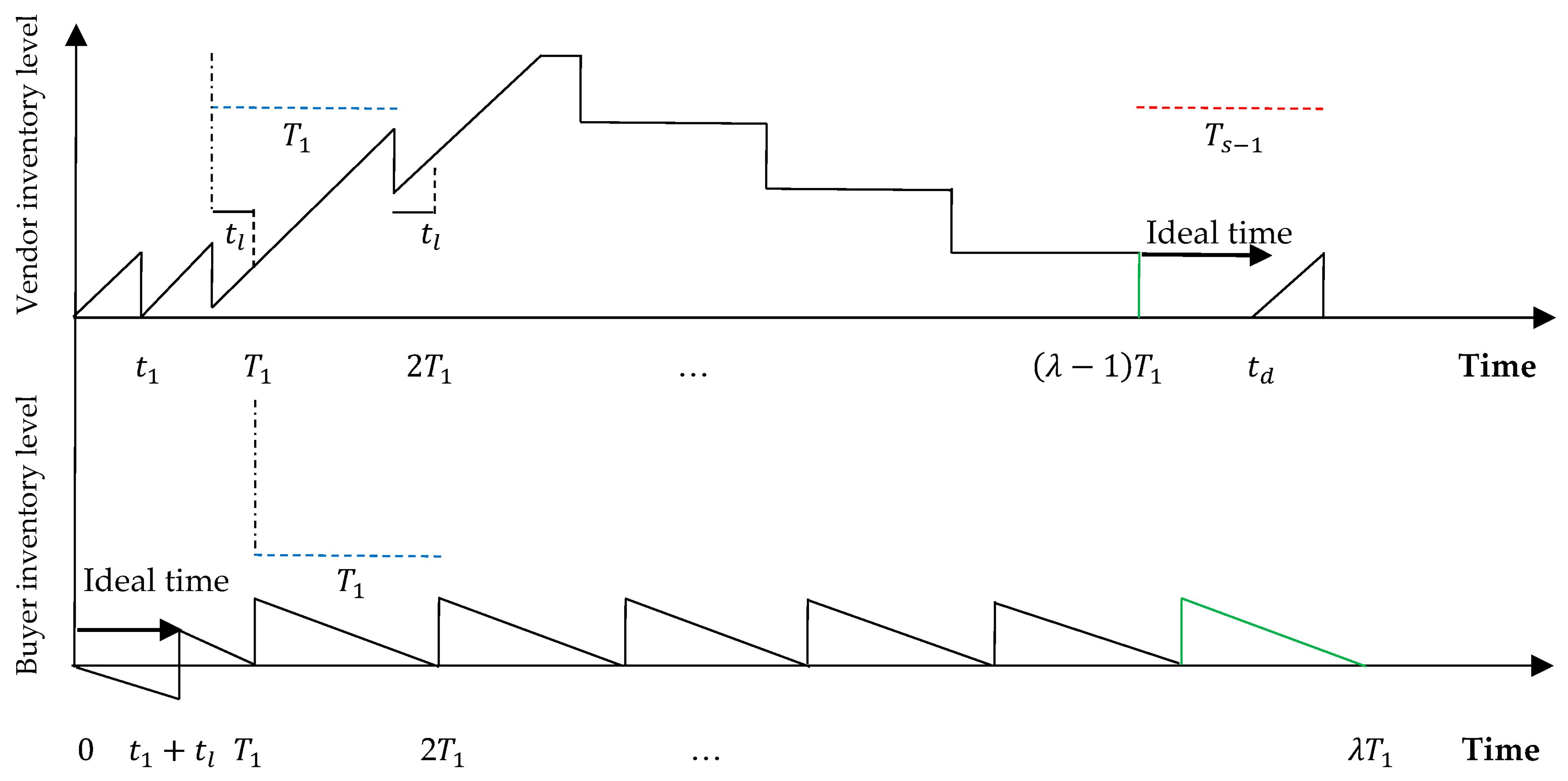
- Any order size of placed at time arrives at the buyer just prior to the depletion of the on-hand inventory of that same period. At the beginning of the production process, the initial inventory at the buyer’s warehouse is zero because no items have been manufactured yet. Accordingly, the first lot size, , is delivered once it has been accumulated from green and regular produced items by time and will reach the buyer after a transportation time . Therefore, in the first period of the first cycle, shortages are allowed and fully backordered by time . Thus, we restrict that in the first cycle, i.e., the second replenishment will reach the buyer’s warehouse before the depletion of the on-hand inventory of the first period, i.e., no later than time .
4.3. The Mathematical Formulation of the Joint Model
4.3.1. The Mathematical Formulation of the First Cycle
4.3.2. The Mathematical Formulation of the Subsequent Cycles
5. Numerical Examples
5.1. Example 1
Remark
5.2. Example 2
5.3. Example 3
5.4. Example 4
5.5. Example 5
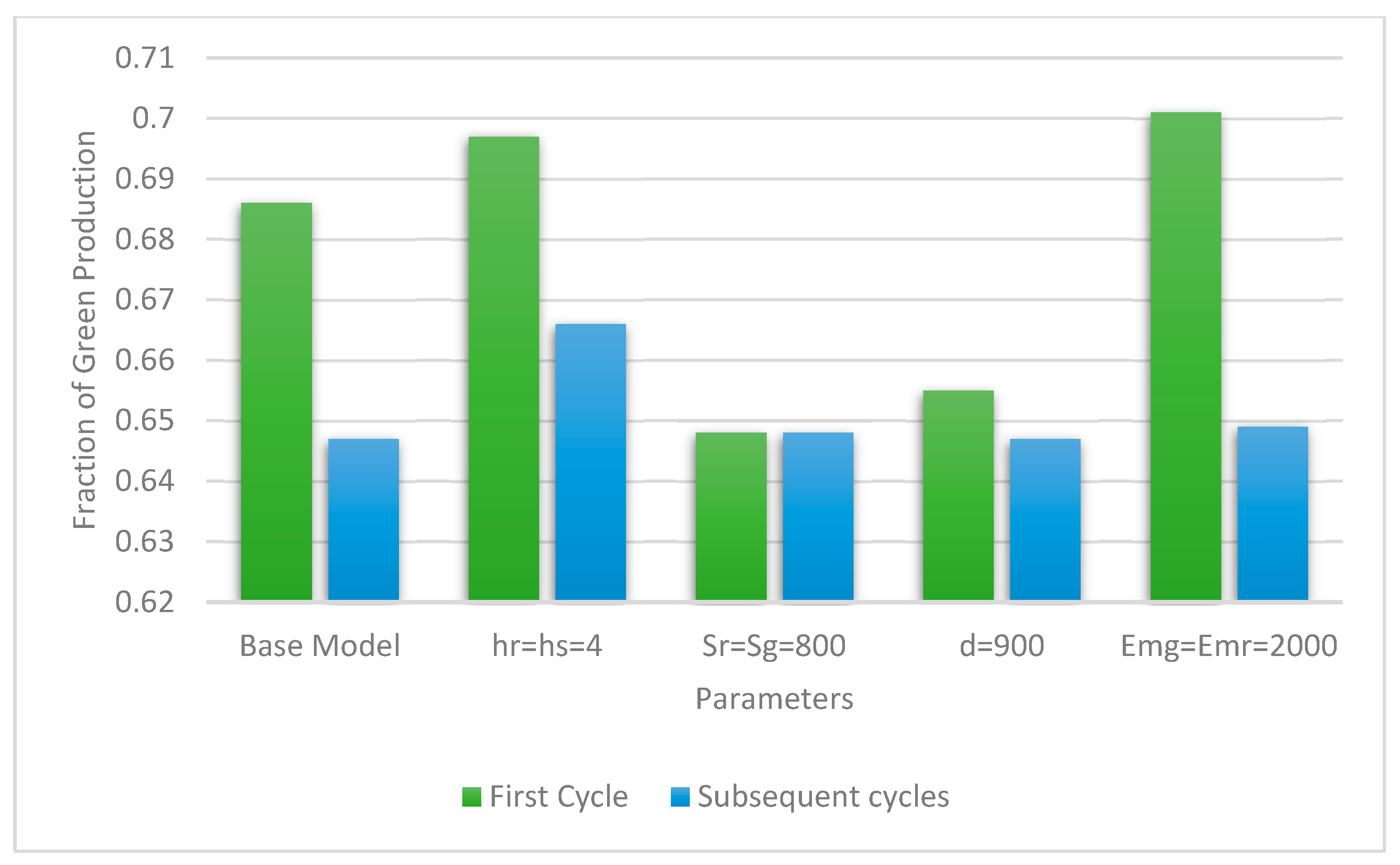
5.6. Example 6
6. Summary of Implications and Managerial Insights
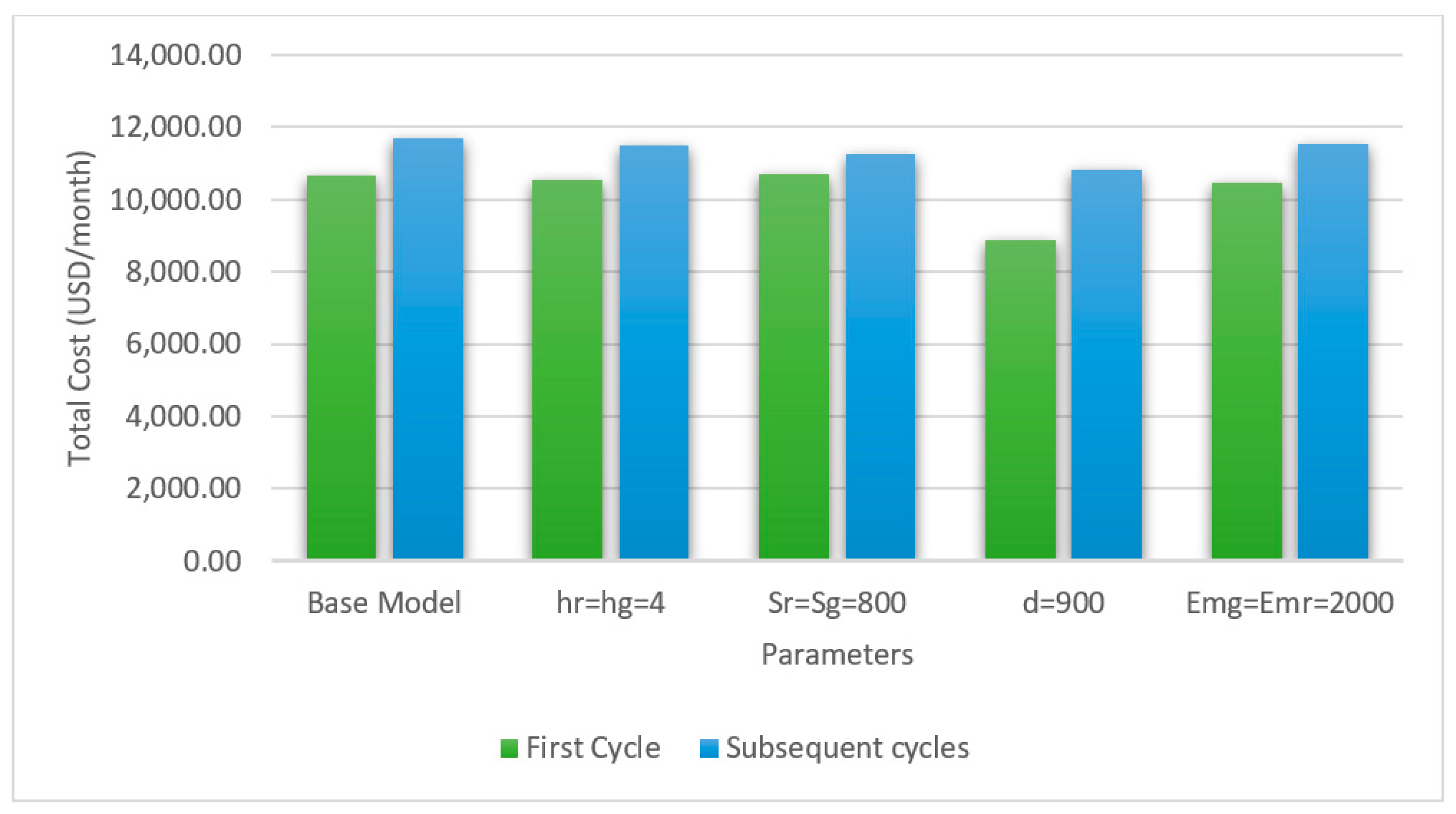
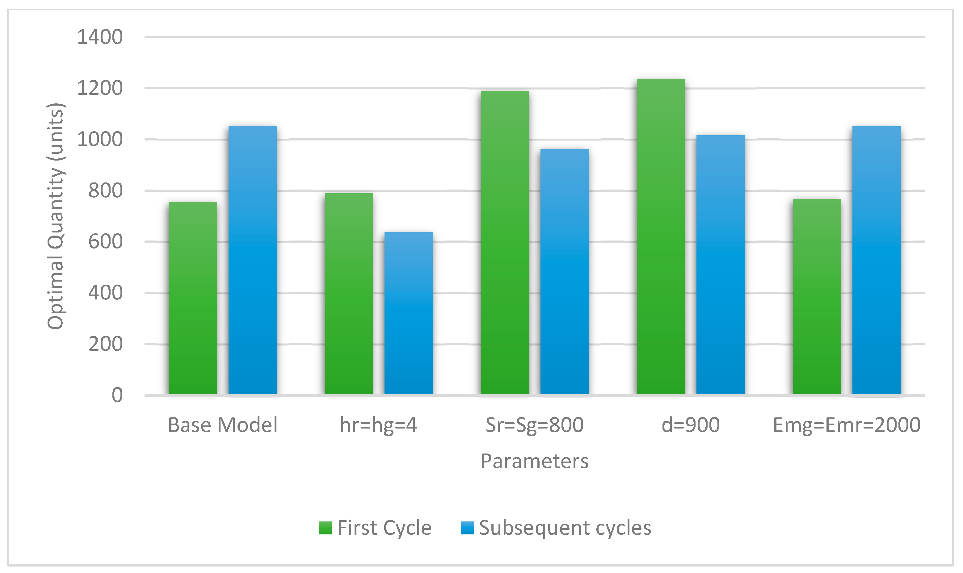
- Unlike the classical JELS inventory model that generates an equal production quantity in all cycles, the proposed model distinguishes the first cycle from subsequent cycles.
- Two mathematical models that reflect the behavior of the first and subsequent cycles are developed. The first model derives distinct optimal results associated with the first cycle, while the other generates distinct optimal results for subsequent cycles.
- In the first time interval, the initial on-hand inventory is zero at the buyer’s warehouse since no items have been produced yet.
- Each subsequent cycle can be associated with its distinct input parameters to ensure that it is independent from the previous one.
- The proposed model allows for the adjustment of the input parameters for any subsequent cycle.
- The model remains viable for subsequent cycles and keeps generating optimal results subject to the desired adjustment of any model parameter as a response to the dynamic nature of demand rate and/or price fluctuation. Such adjustment may also reflect situations such as implementing an alternative policy resulting from acquiring new knowledge, periodic review applications, or machine maintenance scheduling activities that may oblige a decision maker to consider a suitable adjustment of any model parameter.
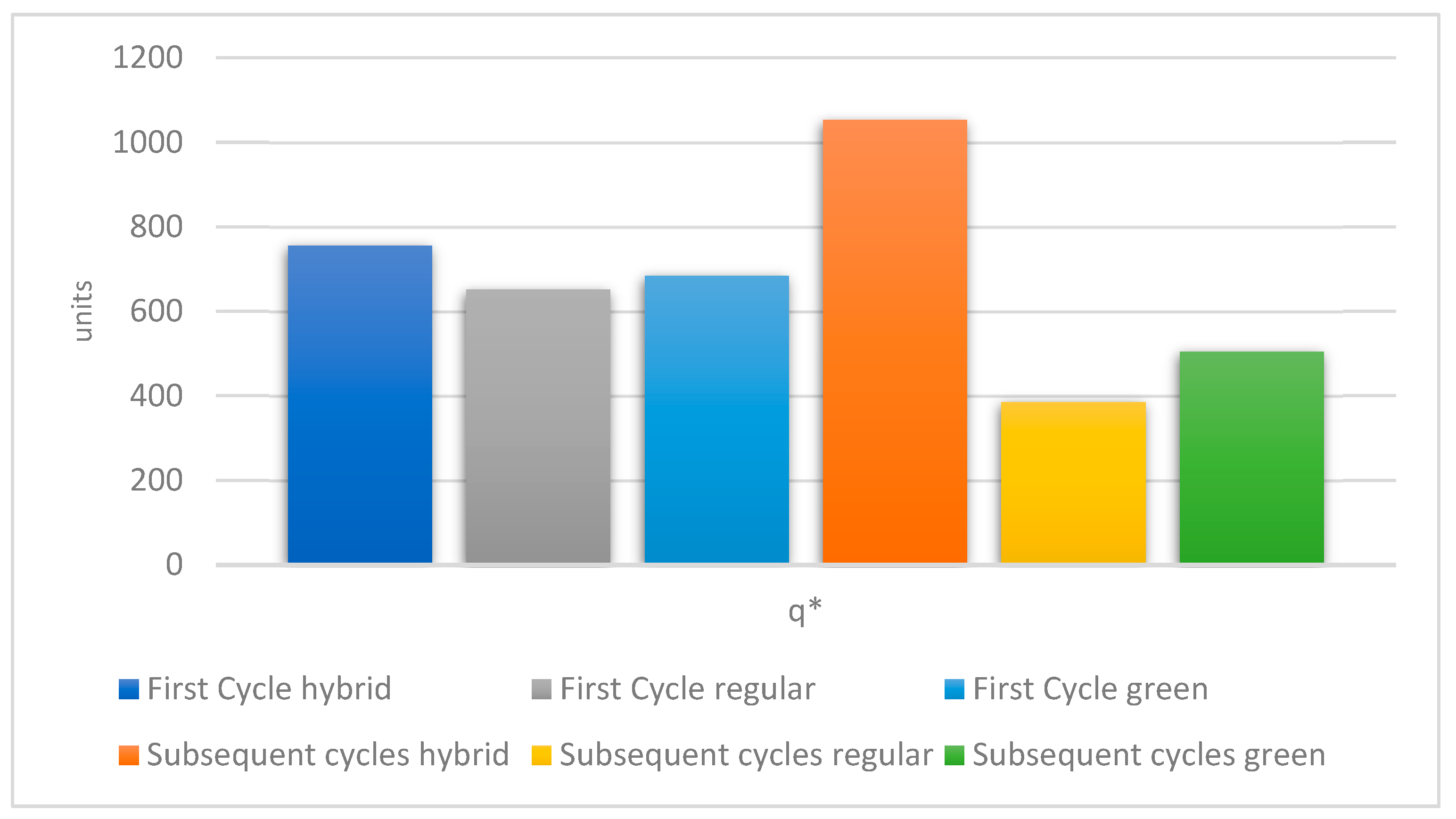
- The developed model accounts for a hybrid production system in its mathematical formulation that simultaneously focuses on green and regular production methods with an optimal allocation fraction of green and regular productions.
- The proposed model considers a mixed transportation policy in its mathematical formulation, which enables a decision maker to combine TL and LTL services to reduce transportation cost.
- The demand is satisfied from a collection of green and regular produced items.
- The proposed model enables a decision maker to trade-off between the production cost and emissions. In this regard, the trade-off is very much related to the emissions penalties for exceeding allowable limits and the unit production cost for green items.
- For subsequent cycles, the production process starts at the time needed for the first lot to be produced and delivered. This, indeed, benefits the vendor by not keeping items for extra time related to the consumption of the last lot at the buyer’s warehouse that has been delivered from previous cycle, which implies further cost reduction.
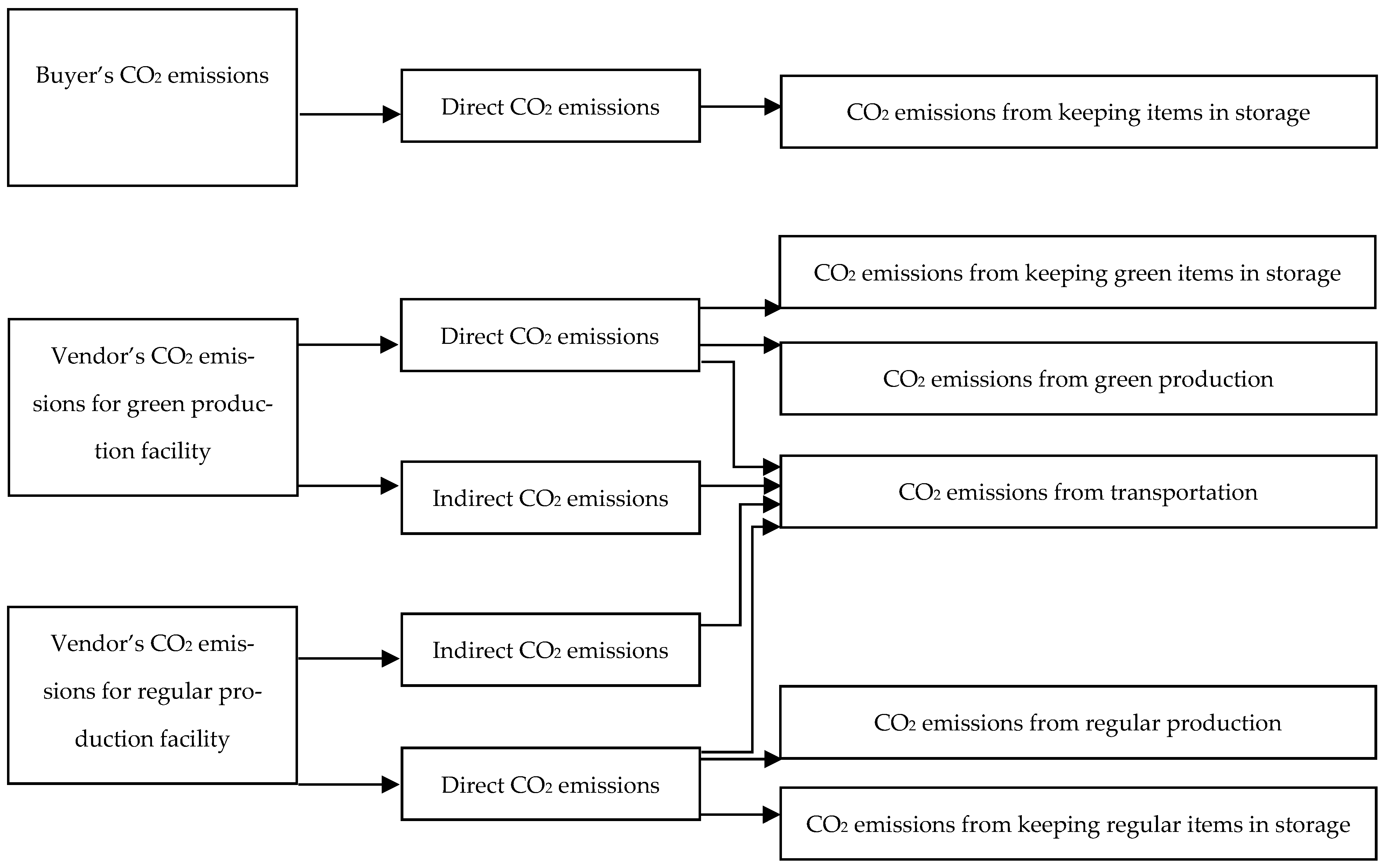
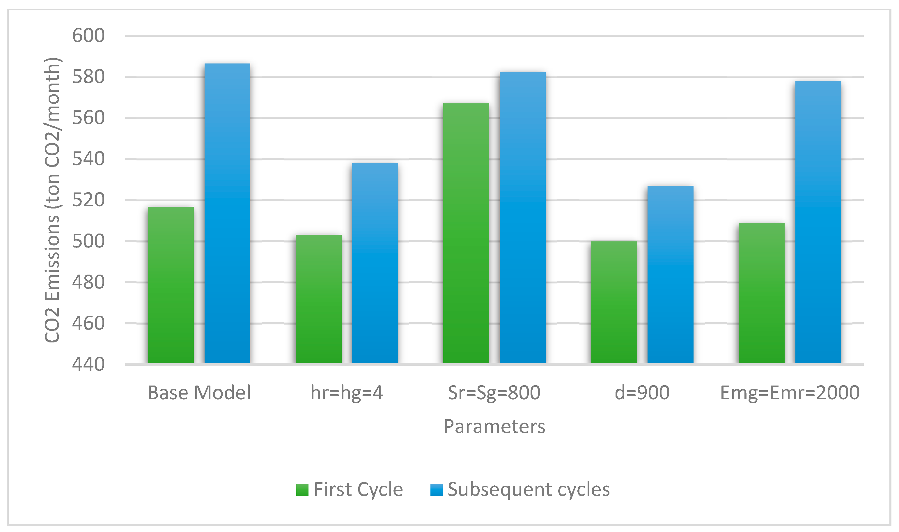
- Emissions are released from production and storage activities related to green and regular produced items along with transportation activity.
- The carbon emissions are relatively associated with carbon taxes and penalties for exceeding the allowable emissions limits. However, the system reaps further cost reduction by selling excess quota in the case that the total emissions are less than that of the emission cap, which reflects the cap-and-trade policy.
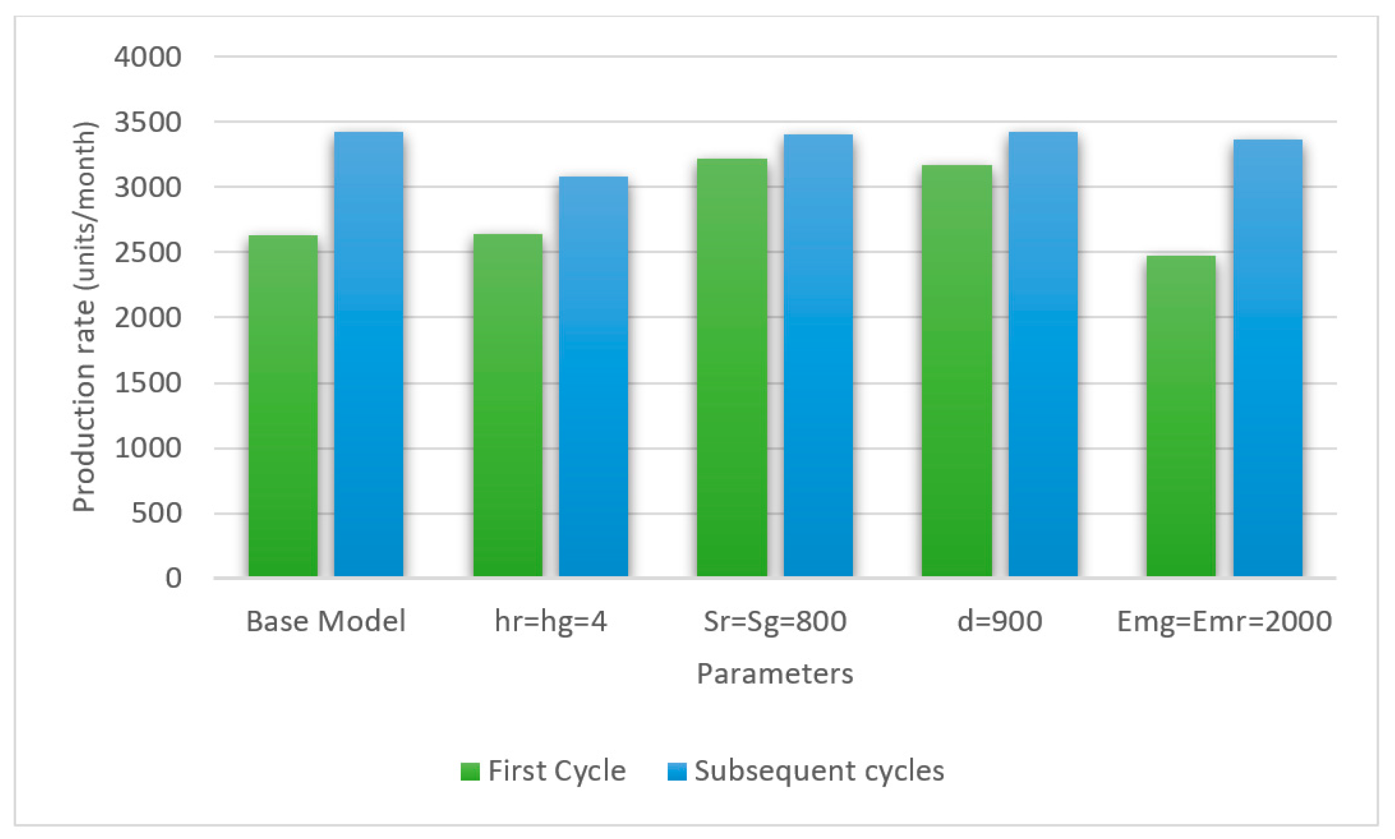
- The base closed-form formula of our model generates optimal values with considerable total system cost reduction, i.e., 33.59% (16.13%) in the first cycle (subsequent cycles) when compared with the existing literature.
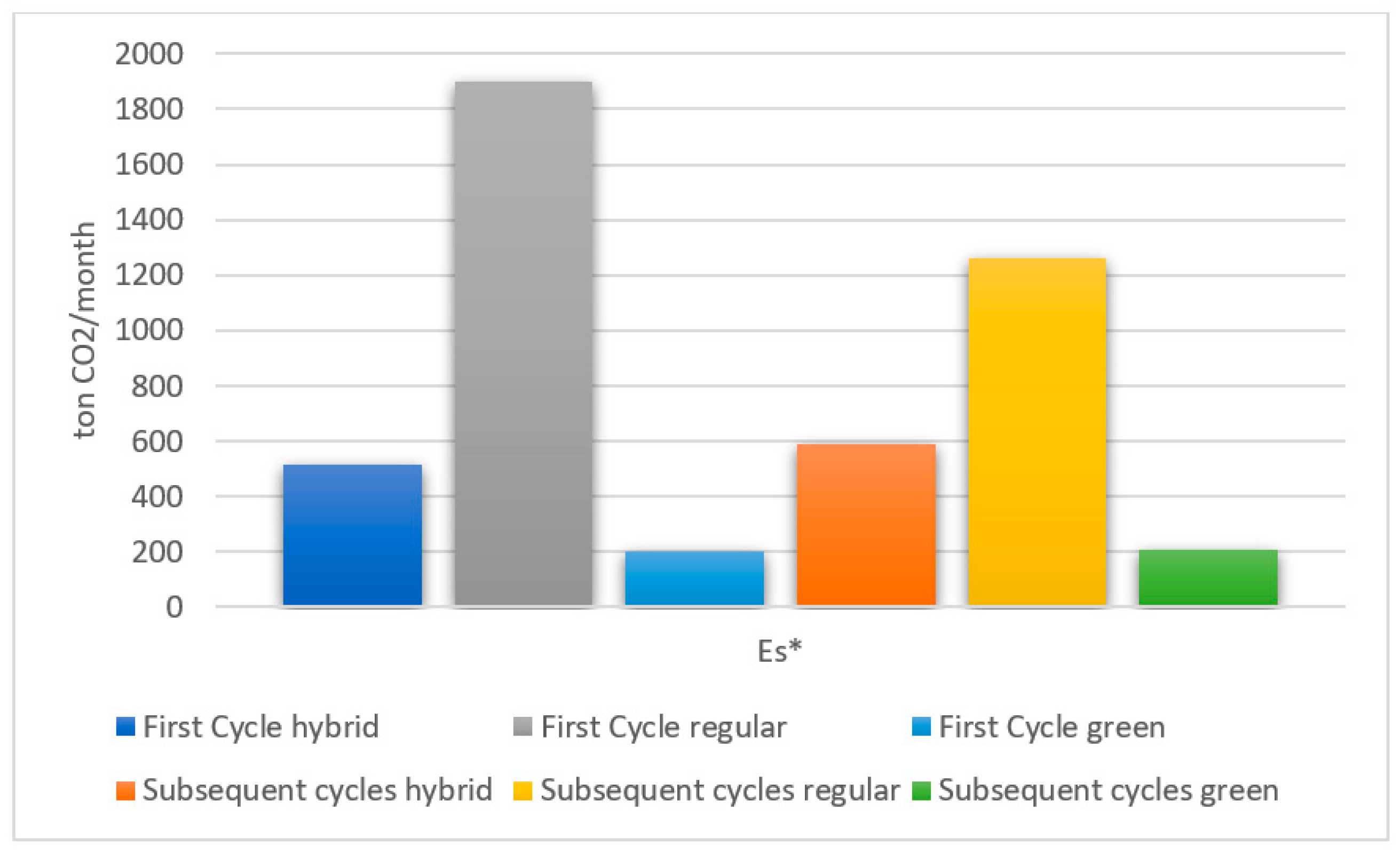
- The optimal production rate generated by the proposed model is the one that minimizes the emissions production function. That is, it generates the lowest emissions possible when compared with the existing literature.
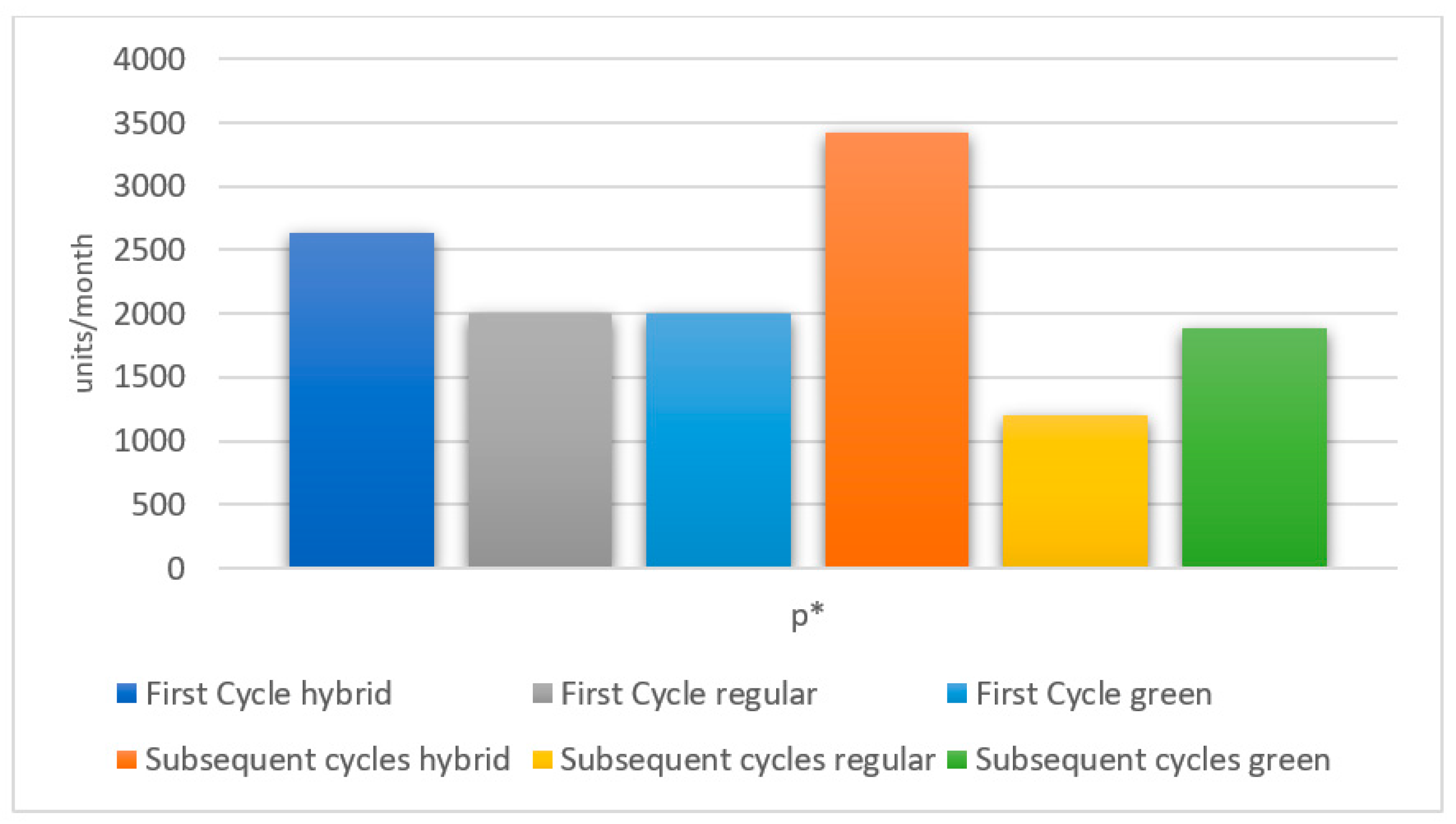
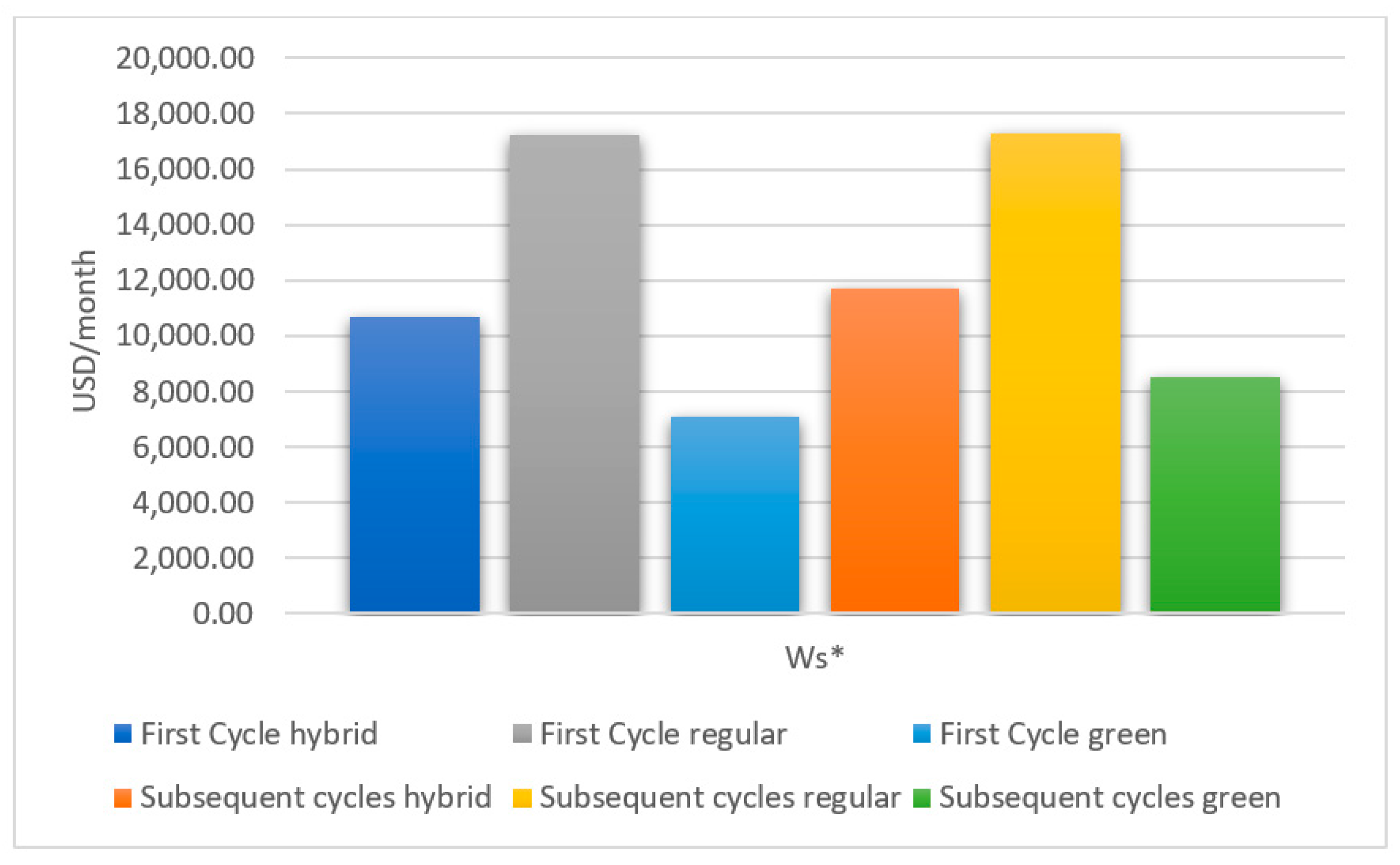
- Adopting a hybrid production method decreases the GHG emissions dramatically, which in turn reduces the minimum total cost per unit time by 38.16% (32.25%) in the first cycle (subsequent cycles) when compared with regular production.
- Adopting a pure green production method decreases the GHG emissions dramatically, which in turn reduces the minimum total cost per unit time by 33.34% (27.41%) in the first cycle (subsequent cycles) when compared with hybrid production. Such savings increase by 58.78% (50.82%) in the first cycle (subsequent cycles) when compared with regular production.
- The total amount of GHG emissions emitted by the system increases (decreases) with demand rate.
7. Conclusions and Further Research
Funding
Data Availability Statement
Acknowledgments
Conflicts of Interest
Appendix A
Appendix A.1. First Cycle (Figure 1)
Appendix A.1.1. Buyer’s Average Inventory Function
Appendix A.1.2. Vendor’s Average Inventory Function
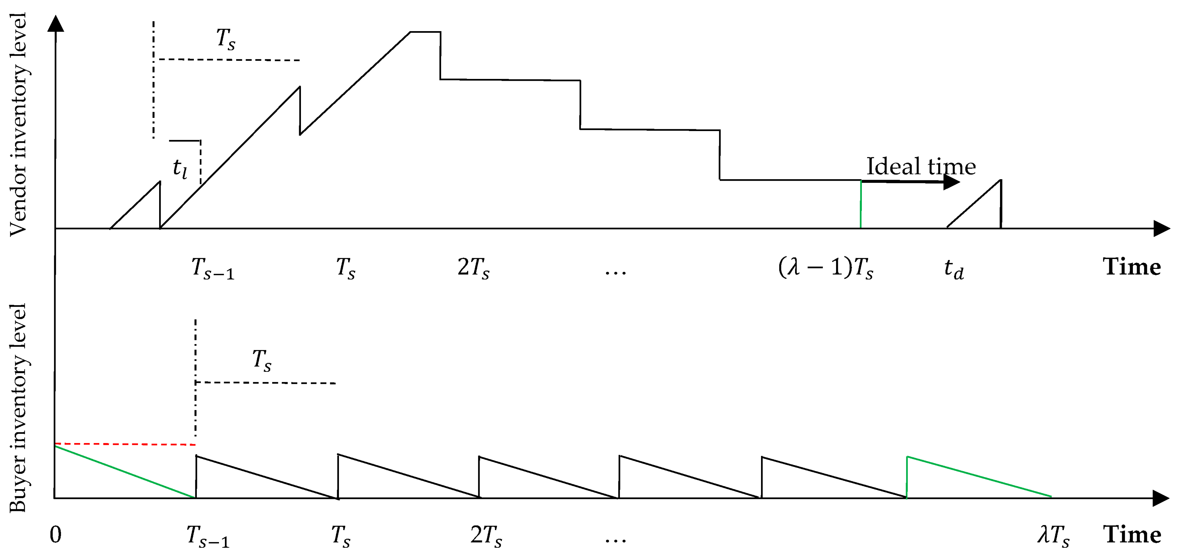
Appendix A.2. Subsequent Cycles (Figure 2)
Appendix A.2.1. Buyer’s Average Inventory Function
Appendix A.2.2. Vendor’s Average Inventory Function
Appendix B
Solution Procedure
References
- Wang, X.J.; Choi, S.H. Impacts of Carbon Emission Reduction Mechanisms on Uncertain Make-To-Order Manufacturing. Int. J. Prod. Res. 2016, 54, 3311–3328. [Google Scholar] [CrossRef]
- Benjaafar, S.; Li, Y.; Daskin, M. Carbon Footprint and the Management of Supply Chains: Insights from Simple Models. IEEE Trans. Autom. Sci. Eng. 2012, 10, 99–116. [Google Scholar] [CrossRef]
- Pachauri, R.K.; Reisinger, A. Climate Change 2007: Synthesis Report. Contribution of Working Groups I, II and III to the Fourth Assessment Report of the Intergovernmental Panel on Climate Change. Climate Change 2007. Working Groups I, II and III to the Fourth Assessment 2007. Available online: https://www.ipcc.ch/site/assets/uploads/2018/02/ar4_syr_full_report.pdf (accessed on 12 August 2023).
- EPA. Carbon Pollution from Transportation. U.S. Environmental Protection Agency. 2022. Available online: https://www.epa.gov/transportation-air-pollution-and-climate-change/carbon-pollution-transportation#transportation (accessed on 12 August 2023).
- Damert, M.; Feng, Y.; Zhu, Q.; Baumgartner, R.J. Motivating Low-Carbon Initiatives among Suppliers: The Role of Risk and Opportunity Perception. Resour Conserv. Recycl. 2018, 136, 276–286. [Google Scholar] [CrossRef]
- Das, C.; Jharkharia, S. Low Carbon Supply Chain: A State-of-the-Art Literature Review. J. Manuf. Technol. Manag. 2018, 29, 398–428. [Google Scholar] [CrossRef]
- Phouratsamay, S.-L.; Cheng, T.C.E. The Single-Item Lot-Sizing Problem with Two Production Modes, Inventory Bounds, and Periodic Carbon Emissions Capacity. Oper. Res. Lett. 2019, 47, 339–343. [Google Scholar] [CrossRef]
- Gong, X.; Zhou, S.X. Optimal Production Planning with Emissions Trading. Oper. Res. 2013, 61, 908–924. [Google Scholar] [CrossRef]
- Hong, Z.; Chu, C.; Yu, Y. Dual-Mode Production Planning for Manufacturing with Emission Constraints. Eur. J. Oper. Res. 2016, 251, 96–106. [Google Scholar] [CrossRef]
- Utama, D.M.; Santoso, I.; Hendrawan, Y.; Dania, W.A.P. Integrated Procurement-Production Inventory Model in Supply Chain: A Systematic Review. Oper. Res. Perspect. 2022, 9, 100221. [Google Scholar] [CrossRef]
- Devy, N.L.; Ai, T.J.; Astanti, R.D. A Joint Replenishment Inventory Model with Lost Sales. In Proceedings of the IOP Conference Series: Materials Science and Engineering; IOP Publishing: Bristol, UK, 2018; Volume 337, p. 12018. [Google Scholar]
- Dong, Y.; Xu, K. A Supply Chain Model of Vendor Managed Inventory. Transp. Res. E Logist. Transp. Rev. 2002, 38, 75–95. [Google Scholar] [CrossRef]
- Banerjee, A. A Joint Economic-lot-size Model for Purchaser and Vendor. Decis. Sci. 1986, 17, 292–311. [Google Scholar] [CrossRef]
- Schaefer, B.; Konur, D. Economic and Environmental Considerations in a Continuous Review Inventory Control System with Integrated Transportation Decisions. Transp. Res. E Logist. Transp. Rev. 2015, 80, 142–165. [Google Scholar] [CrossRef]
- Hovelaque, V.; Bironneau, L. The Carbon-Constrained EOQ Model with Carbon Emission Dependent Demand. Int. J. Prod. Econ. 2015, 164, 285–291. [Google Scholar] [CrossRef]
- Bouchery, Y.; Ghaffari, A.; Jemai, Z.; Dallery, Y. Including Sustainability Criteria into Inventory Models. Eur. J. Oper. Res. 2012, 222, 229–240. [Google Scholar] [CrossRef]
- Gunasekaran, A.; Irani, Z.; Papadopoulos, T. Modelling and Analysis of Sustainable Operations Management: Certain Investigations for Research and Applications. J. Oper. Res. Soc. 2014, 65, 806–823. [Google Scholar] [CrossRef]
- Taleizadeh, A.A.; Soleymanfar, V.R.; Govindan, K. Sustainable Economic Production Quantity Models for Inventory Systems with Shortage. J. Clean Prod. 2018, 174, 1011–1020. [Google Scholar] [CrossRef]
- Montabon, F.; Pagell, M.; Wu, Z. Making Sustainability Sustainable. J. Supply Chain. Manag. 2016, 52, 11–27. [Google Scholar] [CrossRef]
- Goyal, S.K. An Integrated Inventory Model for a Single Supplier-Single Customer Problem. Int. J. Prod. Res. 1977, 15, 107–111. [Google Scholar] [CrossRef]
- Wahab, M.I.M.; Mamun, S.M.H.; Ongkunaruk, P. EOQ Models for a Coordinated Two-Level International Supply Chain Considering Imperfect Items and Environmental Impact. Int. J. Prod. Econ. 2011, 134, 151–158. [Google Scholar] [CrossRef]
- Hua, G.; Cheng, T.C.E.; Wang, S. Managing Carbon Footprints in Inventory Management. Int. J. Prod. Econ. 2011, 132, 178–185. [Google Scholar] [CrossRef]
- Wangsa, I. Greenhouse Gas Penalty and Incentive Policies for a Joint Economic Lot Size Model with Industrial and Transport Emissions. Int. J. Ind. Eng. Comput. 2017, 8, 453–480. [Google Scholar]
- Ben-Daya, M.; Hariga, M. Integrated Single Vendor Single Buyer Model with Stochastic Demand and Variable Lead Time. Int. J. Prod. Econ. 2004, 92, 75–80. [Google Scholar] [CrossRef]
- Hariga, M.; As’ad, R.; Shamayleh, A. Integrated Economic and Environmental Models for a Multi Stage Cold Supply Chain under Carbon Tax Regulation. J. Clean Prod. 2017, 166, 1357–1371. [Google Scholar] [CrossRef]
- Gautam, P.; Kishore, A.; Khanna, A.; Jaggi, C.K. Strategic Defect Management for a Sustainable Green Supply Chain. J. Clean Prod. 2019, 233, 226–241. [Google Scholar] [CrossRef]
- Halat, K.; Hafezalkotob, A. Modeling Carbon Regulation Policies in Inventory Decisions of a Multi-Stage Green Supply Chain: A Game Theory Approach. Comput. Ind. Eng. 2019, 128, 807–830. [Google Scholar] [CrossRef]
- Khouja, M.; Mehrez, A. An Economic Production Lot Size Model with Imperfect Quality and Variable Production Rate. J. Oper. Res. Soc. 1994, 45, 1405–1417. [Google Scholar] [CrossRef]
- Eiamkanchanalai, S.; Banerjee, A. Production Lot Sizing with Variable Production Rate and Explicit Idle Capacity Cost. Int. J. Prod. Econ. 1999, 59, 251–259. [Google Scholar] [CrossRef]
- Ghosh, A.; Jha, J.K.; Sarmah, S.P. Optimal Lot-Sizing under Strict Carbon Cap Policy Considering Stochastic Demand. Appl. Math Model. 2017, 44, 688–704. [Google Scholar] [CrossRef]
- Saga, R.S.; Jauhari, W.A.; Laksono, P.W.; Dwicahyani, A.R. Investigating Carbon Emissions in a Production-Inventory Model under Imperfect Production, Inspection Errors and Service-Level Constraint. Int. J. Logist. Syst. Manag. 2019, 34, 29–55. [Google Scholar] [CrossRef]
- Huang, Y.-S.; Fang, C.-C.; Lin, Y.-A. Inventory Management in Supply Chains with Consideration of Logistics, Green Investment and Different Carbon Emissions Policies. Comput. Ind. Eng. 2020, 139, 106207. [Google Scholar] [CrossRef]
- Chen, X.; Benjaafar, S.; Elomri, A. The Carbon-Constrained EOQ. Oper. Res. Lett. 2013, 41, 172–179. [Google Scholar] [CrossRef]
- Ganesh Kumar, M.; Uthayakumar, R. Modelling on Vendor-Managed Inventory Policies with Equal and Unequal Shipments under GHG Emission-Trading Scheme. Int. J. Prod. Res. 2019, 57, 3362–3381. [Google Scholar] [CrossRef]
- Zanoni, S.; Mazzoldi, L.; Jaber, M.Y. Vendor-Managed Inventory with Consignment Stock Agreement for Single Vendor–Single Buyer under the Emission-Trading Scheme. Int. J. Prod. Res. 2014, 52, 20–31. [Google Scholar] [CrossRef]
- Jaber, M.Y.; Glock, C.H.; El Saadany, A.M.A. Supply Chain Coordination with Emissions Reduction Incentives. Int. J. Prod. Res. 2013, 51, 69–82. [Google Scholar] [CrossRef]
- Turken, N.; Geda, A.; Takasi, V.D.G. The Impact of Co-Location in Emissions Regulation Clusters on Traditional and Vendor Managed Supply Chain Inventory Decisions. Ann. Oper. Res. 2021, 1–50. [Google Scholar] [CrossRef]
- Bazan, E.; Jaber, M.Y.; Zanoni, S. Supply Chain Models with Greenhouse Gases Emissions, Energy Usage and Different Coordination Decisions. Appl. Math Model 2015, 39, 5131–5151. [Google Scholar] [CrossRef]
- Astanti, R.D.; Daryanto, Y.; Dewa, P.K. Low-Carbon Supply Chain Model under a Vendor-Managed Inventory Partnership and Carbon Cap-and-Trade Policy. J. Open Innov. Technol. Mark. Complex. 2022, 8, 30. [Google Scholar] [CrossRef]
- Malik, A.I.; Kim, B.S. A Constrained Production System Involving Production Flexibility and Carbon Emissions. Mathematics 2020, 8, 275. [Google Scholar] [CrossRef]
- Jauhari, W.A.; Pujawan, I.N.; Suef, M.; Govindan, K. Low Carbon Inventory Model for Vendor-buyer System with Hybrid Production and Adjustable Production Rate under Stochastic Demand. Appl. Math Model 2022, 108, 840–868. [Google Scholar] [CrossRef]
- Sarkar, B.; Saren, S. Product Inspection Policy for an Imperfect Production System with Inspection Errors and Warranty Cost. Eur. J. Oper. Res. 2016, 248, 263–271. [Google Scholar] [CrossRef]
- Rad, M.A.; Khoshalhan, F.; Glock, C.H. Optimal Production and Distribution Policies for a Two-Stage Supply Chain with Imperfect Items and Price-and Advertisement-Sensitive Demand: A Note. Appl. Math Model 2018, 57, 625–632. [Google Scholar] [CrossRef]
- Kim, M.-S.; Kim, J.-S.; Sarkar, B.; Sarkar, M.; Iqbal, M.W. An Improved Way to Calculate Imperfect Items during Long-Run Production in an Integrated Inventory Model with Backorders. J. Manuf. Syst. 2018, 47, 153–167. [Google Scholar] [CrossRef]
- De Giovanni, P.; Karray, S.; Martín-Herrán, G. Vendor Management Inventory with Consignment Contracts and the Benefits of Cooperative Advertising. Eur. J. Oper. Res. 2019, 272, 465–480. [Google Scholar] [CrossRef]
- Phan, D.A.; Vo, T.L.H.; Lai, A.N.; Nguyen, T.L.A. Coordinating Contracts for VMI Systems under Manufacturer-CSR and Retailer-Marketing Efforts. Int. J. Prod. Econ. 2019, 211, 98–118. [Google Scholar] [CrossRef]
- Ben-Daya, M.; As’ad, R.; Nabi, K.A. A Single-Vendor Multi-Buyer Production Remanufacturing Inventory System under a Centralized Consignment Arrangement. Comput. Ind. Eng. 2019, 135, 10–27. [Google Scholar] [CrossRef]
- Tarhini, H.; Karam, M.; Jaber, M.Y. An Integrated Single-Vendor Multi-Buyer Production Inventory Model with Transshipments between Buyers. Int. J. Prod. Econ. 2020, 225, 107568. [Google Scholar] [CrossRef]
- Dey, O.; Giri, B.C. A New Approach to Deal with Learning in Inspection in an Integrated Vendor-Buyer Model with Imperfect Production Process. Comput. Ind. Eng. 2019, 131, 515–523. [Google Scholar] [CrossRef]
- Giri, B.C.; Chakraborty, A.; Maiti, T. Consignment Stock Policy with Unequal Shipments and Process Unreliability for a Two-Level Supply Chain. Int. J. Prod. Res. 2017, 55, 2489–2505. [Google Scholar] [CrossRef]
- Jauhari, W.A.; Sofiana, A.; Kurdhi, N.A.; Laksono, P.W. An Integrated Inventory Model for Supplier-Manufacturer-Retailer System with Imperfect Quality and Inspection Errors. Int. J. Logist. Syst. Manag. 2016, 24, 383–407. [Google Scholar]
- Khan, M.; Hussain, M.; Cárdenas-Barrón, L.E. Learning and Screening Errors in an EPQ Inventory Model for Supply Chains with Stochastic Lead Time Demands. Int. J. Prod. Res. 2017, 55, 4816–4832. [Google Scholar] [CrossRef]
- Pal, S.; Mahapatra, G.S. A Manufacturing-Oriented Supply Chain Model for Imperfect Quality with Inspection Errors, Stochastic Demand under Rework and Shortages. Comput. Ind. Eng. 2017, 106, 299–314. [Google Scholar] [CrossRef]
- Tiwari, S.; Kazemi, N.; Modak, N.M.; Cárdenas-Barrón, L.E.; Sarkar, S. The Effect of Human Errors on an Integrated Stochastic Supply Chain Model with Setup Cost Reduction and Backorder Price Discount. Int. J. Prod. Econ. 2020, 226, 107643. [Google Scholar] [CrossRef]
- Jaggi, C.K.; Tiwari, S.; Shafi, A.A. Effect of Deterioration on Two-Warehouse Inventory Model with Imperfect Quality. Comput. Ind. Eng. 2015, 88, 378–385. [Google Scholar] [CrossRef]
- Alamri, A.A. Carbon Emissions Effect on Vendor-Managed Inventory System Considering Displaced Re-Start-Up Production Time. Logistics 2023, 7, 67. [Google Scholar] [CrossRef]
- Konur, D. Carbon Constrained Integrated Inventory Control and Truckload Transportation with Heterogeneous Freight Trucks. Int. J. Prod. Econ. 2014, 153, 268–279. [Google Scholar] [CrossRef]
- Bouchery, Y.; Ghaffari, A.; Jemai, Z.; Tan, T. Impact of Coordination on Costs and Carbon Emissions for a Two-Echelon Serial Economic Order Quantity Problem. Eur. J. Oper. Res. 2017, 260, 520–533. [Google Scholar] [CrossRef]
- Alamri, A.A. A Sustainable Closed-Loop Supply Chains Inventory Model Considering Optimal Number of Remanufacturing Times. Sustainability 2023, 15, 9517. [Google Scholar] [CrossRef]
- Alamri, A.A. Exploring the Effect of the First Cycle on the Economic Production Quantity Repair and Waste Disposal Model. Appl. Math Model 2021, 89, 519–540. [Google Scholar] [CrossRef]
- Lippman, S.A. Economic Order Quantities and Multiple Set-up Costs. Manag. Sci. 1971, 18, 39–47. [Google Scholar] [CrossRef]
- Venkatachalam, S.; Narayanan, A. Efficient Formulation and Heuristics for Multi-Item Single Source Ordering Problem with Transportation Cost. Int. J. Prod. Res. 2016, 54, 4087–4103. [Google Scholar] [CrossRef]
- Kazemi, N.; Abdul-Rashid, S.H.; Ghazilla, R.A.R.; Shekarian, E.; Zanoni, S. Economic Order Quantity Models for Items with Imperfect Quality and Emission Considerations. Int. J. Syst. Sci. Oper. Logist. 2018, 5, 99–115. [Google Scholar] [CrossRef]
- Fandel, G. Production and Cost Theory; Springer: Berlin/Heidelberg, Germany, 1991; Volume 10, pp. 973–978. [Google Scholar]
- Narita, H. Environmental Burden Analyzer for Machine Tool Operations and Its Application. In Manufacturing System; InTech Europe: Rijeka, Croatia, 2012; pp. 247–260. [Google Scholar]
- Stewart, G.W. Introduction to Matrix Computations, Computer Science and Applied Mathematics; Academic Press: New York, NY, USA, 1973. [Google Scholar]
- Balkhi, Z.T.; Benkherouf, L. A Production Lot Size Inventory Model for Deteriorating Items and Arbitrary Production and Demand Rates. Eur. J. Oper. Res. 1996, 92, 302–309. [Google Scholar] [CrossRef]
- Emet, S. An Mixed Integer Approach for Optimizing Production Planning. In Proceedings of the 13th WSEAS International Conference on Applied Mathematics, Puerto De La Cruz, Spain, 15–17 December 2008; pp. 361–364. [Google Scholar]
- Alamri, A.A. Theory and Methodology on the Global Optimal Solution to a General Reverse Logistics Inventory Model for Deteriorating Items and Time-Varying Rates. Comput. Ind. Eng. 2011, 60, 236–247. [Google Scholar] [CrossRef]


| No | Authors | First Cycle | Adjustable Parameters | Adjustable Production Rate | Hybrid Production | Emissions | Carbon Regulations |
|---|---|---|---|---|---|---|---|
| 1 | Wahab et al. [21] | Transportation | Carbon tax | ||||
| 2 | Hariga et al. [25] | Storage, transportation | Carbon tax | ||||
| 3 | Jaber et al. [36] | Production | Carbon tax, penalty | ||||
| 4 | Bazan et al. [38] | Production, transportation | Carbon tax, penalty | ||||
| 5 | Kumar and Uthayakumar [34] | Production | Carbon tax, penalty | ||||
| 6 | Zanoni et al. [35] | Production | Carbon tax, penalty | ||||
| 7 | Konur [61] | Transportation | Carbon cap | ||||
| 8 | Astanti et al. [39] | Production, transportation | Carbon tax | ||||
| 9 | Malik and Kim [40] | Production | Carbon tax | ||||
| 10 | Bouchery [56] | Transportation | Carbon tax | ||||
| 11 | Jauhari et al. [41] | Production, transportation, storage | Carbon tax | ||||
| 13 | Alamri [57] | Production, transportation, storage | Carbon tax, carbon cap | ||||
| 14 | Proposed model | Production, transportation, storage | Carbon tax, carbon cap, penalty |
| denotes green production and denotes regular production | |
| refers to the first cycle and refers to the subsequent cycles | |
| The time to produce units | |
| The time to consume units | |
| Cycle time | |
| The time to consume units | |
| The idle time before commencing the production process for subsequent cycles | |
| The lead time (order point) to deliver the order quantity of size | |
| CO2 emissions related to electricity (ton CO2/kWh) | |
| Buyer’s energy consumption for keeping items in storage (kWh/unit/unit time) | |
| Vendor’s energy consumption for keeping items in storage (kWh/unit/unit time) | |
| CO2 emissions related to the buyer’s facility (ton CO2/unit) | |
| Buyer’s CO2 emissions tax ($/ton CO2) | |
| The truck capacity (units/truck) | |
| Fixed transportation cost per truck ($/truck) | |
| Fixed transportation cost per unit ($/unit), where | |
| Product’s weight (ton/unit) | |
| Distance from the freight to the vendor (km) | |
| Distance from the vendor to the buyer (km) | |
| The amount of fuel consumed by an empty truck (liters/km) | |
| The amount of fuel consumed by a truckload (liters/km/ton) | |
| Variable transportation cost associated with fuel consumption ($/liter) | |
| CO2 emissions from truck fuel (ton CO2/liter) | |
| CO2 emissions generated by the vendor’s facility (ton CO2/unit) | |
| The total amount of CO2 emissions (ton CO2/unit), where | |
| CO2 emissions limit (ton CO2/unit time) | |
| CO2 emissions penalty that the system incurs for exceeding emissions limit ($/unit time) | |
| CO2 emissions cap (ton CO2), where | |
| Vendor’s CO2 emissions tax ($/ton CO2) | |
| Vendor’s CO2 emissions revenue earned for selling excess quota ($/ton CO2) | |
| Vendor’s CO2 emissions tax for transportation ($/ton CO2) | |
| CO2 emissions function parameter for production (kg CO2 unit time2/unit3) | |
| CO2 emissions function parameter for production (kg CO2 unit time/unit2) | |
| CO2 emissions function parameter for production (kg CO2/unit) | |
| The per unit time cost to run the machine independent of production rate ($/unit time) | |
| The increase in unit machining cost associated with the increase of one unit in production rate ($ unit time/unit2) | |
| Buyer’s ordering cost | |
| Vendor’s set-up cost | |
| Vendor’s holding cost, where represents the base model | |
| Buyer’s demand rate (units/unit time) | |
| Decision variables: | |
| Vendor’s coordination multiplier, where and is an integer | |
| Vendor’s allocation fraction of green production, where | |
| Production rate (units/unit time), where | |
| Production rate (units/unit time), where and | |
| Order quantity (units), where | |
| Number of trucks required to deliver , where and is an integer |
| 2500 | 2000 | 0.0008 | 0.0004 | 1.6 | 2 |
| USD/month | USD/month | USD month/unit2 | USD month/unit2 | USD/ton CO2 | USD/ton CO2 |
| 0.0026 | 0.064 | 0.32 | 0.01 | 2 | 0.75 |
| ton CO2/liter | liters/km/ton | liters/km | ton/unit | USD/ton CO2 | USD/liter |
| 80 | 300 | 400 | 5 | 4 | 3 |
| km | km | ton CO2/month | USD/unit/month | USD/unit/month | USD/unit/month |
| 0.08 | 2 | 2 | 1000 | 4000 | 1200 |
| month | USD/ton CO2 | USD/ton CO2 | units/month | units/month | units/month |
| 1200 | 800 | 400 | 500 | 300 | 2 |
| USD/set-up | USD/set-up | USD/order | USD/truck | units/truck | USD/unit |
| 0.0000003 | 0.0012 | 1.4 | 0.0000005 | 0.0008 | 1.5 |
| ton CO2 month 2/unit3 | ton CO2 month/unit2 | ton CO2/unit | ton CO2 month 2/unit3 | ton CO2 month/unit2 | ton CO2/unit |
| 1.44 | 1 | 1.44 | 0.0005 | ||
| kWh/unit/month | kWh/unit/month | kWh/unit/month | ton CO2/kWh |
| (ton CO2/Unit Time) | Penalty Scheme | (USD/Unit Time) | |
|---|---|---|---|
| 1 | 400 | 0 | |
| 2 | 500 | 500 | |
| 3 | 600 | 1000 | |
| 4 | 700 | 1500 | |
| 5 | 800 | 2000 | |
| 6 | 800 | 2500 |
| First cycle | Mixed policy | |||||||
| 0.686 | 2635.15 | 755.76 | 2 | 2 | 516.74 | 10,663.86 | ||
| Subsequent cycles | ||||||||
| 0.647 | 3427.72 | 1053.79 | 1 | 3 | 586.39 | 11,697.82 |
| First cycle | Mixed policy | |||||||
| 0.686 | 2635.15 | 755.76 | 2 | 2 | 516.74 | 10,663.86 | ||
| Second cycle | ||||||||
| 0.647 | 3427.72 | 1053.79 | 1 | 3 | 586.39 | 11,697.82 | ||
| Subsequent cycles | ||||||||
| 0.654 | 3102.71 | 667.01 | 2 | 2 | 663.81 | 14,776.23 |
| Parameter | First cycle | Mixed policy | |||||||
| 0.697 | 2644.95 | 789.51 | 2 | 2 | 503.01 | 10,537.37 | |||
| Subsequent cycles | |||||||||
| 0.666 | 3083.21 | 636.70 | 2 | 2 | 537.83 | 11,500.38 | |||
| First cycle | Mixed policy | ||||||||
| 0.648 | 3221.85 | 1189.00 | 1 | 4 | 566.89 | 10,713.34 | |||
| Subsequent cycles | |||||||||
| 0.648 | 3403.90 | 961.65 | 1 | 3 | 582.27 | 11,273.99 | |||
| First cycle | Mixed policy | ||||||||
| 0.655 | 3166.62 | 1235.95 | 1 | 4 | 499.75 | 8862.99 | |||
| Subsequent cycles | |||||||||
| 0.647 | 3423.41 | 1015.44 | 1 | 3 | 526.92 | 10,823.63 | |||
| First cycle | Mixed policy | ||||||||
| 0.701 | 2476.57 | 767.30 | 2 | 2 | 508.67 | 10,468.41 | |||
| Subsequent cycles | |||||||||
| 0.649 | 3367.31 | 1050.79 | 1 | 3 | 577.90 | 11,550.79 |
| First cycle | Mixed policy | Saving due to hybrid production | ||||||
| 2000.00 | 652.06 | 2 | 2 | 1900.08 | 17,245.98 | 38.16% | ||
| Subsequent cycles | ||||||||
| 1200.00 | 385.46 | 4 | 1 | 1261.00 | 17,265.70 | 32.25% |
| First cycle | Mixed policy | Saving compared with hybrid production | Saving compared with regular production | ||||||
| 2000.03 | 684.13 | 2 | 2 | 200.8 | 7108.19 | 33.34% | 58.78% | ||
| Subsequent cycles | |||||||||
| 1889.09 | 504.74 | 2 | 1 | 204.63 | 8491.07 | 27.41% | 50.82% |
| (ton CO2/Unit Time) | Penalty Scheme | (USD/Unit Time) | |
|---|---|---|---|
| 1 | 220 | 0 | |
| 2 | 330 | 1000 | |
| 3 | 440 | 2000 | |
| 4 | 550 | 3000 | |
| 5 | 600 | 4000 | |
| 6 | 600 | 5000 |
Disclaimer/Publisher’s Note: The statements, opinions and data contained in all publications are solely those of the individual author(s) and contributor(s) and not of MDPI and/or the editor(s). MDPI and/or the editor(s) disclaim responsibility for any injury to people or property resulting from any ideas, methods, instructions or products referred to in the content. |
© 2023 by the author. Licensee MDPI, Basel, Switzerland. This article is an open access article distributed under the terms and conditions of the Creative Commons Attribution (CC BY) license (https://creativecommons.org/licenses/by/4.0/).
Share and Cite
Alamri, A.A. Efficient Formulation for Vendor–Buyer System Considering Optimal Allocation Fraction of Green Production. Axioms 2023, 12, 1104. https://doi.org/10.3390/axioms12121104
Alamri AA. Efficient Formulation for Vendor–Buyer System Considering Optimal Allocation Fraction of Green Production. Axioms. 2023; 12(12):1104. https://doi.org/10.3390/axioms12121104
Chicago/Turabian StyleAlamri, Adel A. 2023. "Efficient Formulation for Vendor–Buyer System Considering Optimal Allocation Fraction of Green Production" Axioms 12, no. 12: 1104. https://doi.org/10.3390/axioms12121104
APA StyleAlamri, A. A. (2023). Efficient Formulation for Vendor–Buyer System Considering Optimal Allocation Fraction of Green Production. Axioms, 12(12), 1104. https://doi.org/10.3390/axioms12121104