Residuated Basic Logic

Abstract

Residuated basic logic ($\mathsf{RBL}$) is the logic of residuated basic algebras, which constitutes a conservative extension of basic propositional logic ($\mathsf{BPL}$). The basic implication is a residual of a non-associative binary operator in $\mathsf{RBL}$. The conservativity is shown by relational semantics. A Gentzen-style sequent calculus $\mathsf{GRBL}$, which is an extension of the distributive full non-associative Lambek calculus, is established for residuated basic logic. The calculus $\mathsf{GRBL}$ admits the mix-elimination, subformula, and disjunction properties. Moreover, the class of all residuated basic algebras has the finite embeddability property. The consequence relation of $\mathsf{GRBL}$ is decidable.

1. Introduction

The term ‘subintuitionistic logic’, as described in [1,2], covers logics in the language of intuitionistic logic ($\mathsf{Int}$) that are defined in the same manner as intuitionistic logic but lack some conditions on the Kripke semantics. Basic propositional logic ($\mathsf{BPL}$), which was introduced by Visser [3], is the subintuitionistic logic characterized by the class of all transitive frames. It is well known that $\mathsf{Int}$ is embedded into the modal logic $\mathsf{S}\mathsf{4}$ via the Gödel-McKinsey-Tarski translation (see, e.g., [4]). It is also known that $\mathsf{BPL}$ is embeddable into the modal logic $\mathsf{K}\mathsf{4}$ ([1,3,5,6]). Basic propositional logic exists in the common part of $\mathsf{Int}$ and Visser’s formal provability logic $\mathsf{FPL}$. Visser [3] observed that $\mathsf{FPL}$ is embeddable into the Gödel-Löb modal logic $\mathsf{GL}$, which is incomparable with the modal logic $\mathsf{S}\mathsf{4}$. In the modal respect, the modal logic $\mathsf{K}\mathsf{4}$ exists in the common part of $\mathsf{S}\mathsf{4}$ and $\mathsf{GL}$. Hence, the role of $\mathsf{BPL}$ as a basis for $\mathsf{FPL}$ and $\mathsf{Int}$ is analogous to the role of $\mathsf{K}\mathsf{4}$ as the basis for $\mathsf{S}\mathsf{4}$ and $\mathsf{GL}$.

Basic propositional logic is a significant form of constructive logic. Ruitenburg [7] commented that a truly constructive logic should admit an interpretation that is non-circular and constructive in itself. Intuitionistic calculus does not satisfy this constraint. Gentzen [8] observed that the Brouwer-Heyting-Kolmogorov (BHK) interpretation of intuitionistic logic is circular in the proof semantics of implication. For example, to understand the meaning of the claim that a is a proof of $\alpha \to \beta$ in the sense of the BHK interpretation, implication elimination is equivalent to the full modus ponens axiom $\alpha \wedge (\alpha \to \beta )⊢\beta$. In this case, the existence of a proof of $\beta$ from $\alpha$ involves implication by the assumption $\alpha \to \beta$, and hence the interpretation of the implication is circular. Ruitenburg [7] developed the truly constructive logic $\mathsf{BPC}$ (basic propositional calculus), which is not circular and turns out to be equivalent to Visser’s natural deduction system for $\mathsf{BPL}$. The Kripke semantics for $\mathsf{BPL}$ were originally given by Visser [3], while the soundness and completeness of $\mathsf{BPC}$ under the Kripke semantics were presented by Ardeshir and Ruitenburg [9,10].

Visser’s propositional logics have been studied in, e.g., [6,9,10,11,12,13]. In the proof-theoretic respect, Gentzen-style sequent calculi for basic propositional logics are given in [14,15,16,17]. In this paper, we shall study $\mathsf{BPC}$ from the perspective of substructural logics. Substructural logics are logics that drop some structural rules in sequent formalizations. Many well-known logics are substructural, such as Lambek calculus, ukasiewicz many-valued logics and relevant logics. Algebras for substructural logics are given by residuated lattices [18,19,20,21]. We shall introduce residuation into $\mathsf{BPL}$. The basic implication in $\mathsf{BPL}$ is that there is no right residual of any binary operator in the language of $\mathsf{BPL}$. Thus, we introduce a new binary operator • (product), which satisfies additional conditions such that the basic implication is a residual of the product. The resulting logic is called residuated basic logic ($\mathsf{RBL}$). Algebras for $\mathsf{RBL}$ are defined as bounded distributive lattices with residuation pairs $(•,\to )$ and $(•,\leftarrow )$, where • satisfies the conditions of weakening and strong contraction. We prove that the basic sequent system for $\mathsf{RBL}$ is a conservative extension of $\mathsf{BPC}$.

In the present paper, the Gentzen-style sequent calculus $\mathsf{GRBL}$ will be established for $\mathsf{RBL}$. This calculus is obtained from the distributive full non-associative Lambek calculus ($\mathsf{DFNL}$) by adding the structural rules of weakening and strong contraction. $\mathsf{DFNL}$ is obtained from the full non-associative Lambek calculus ($\mathsf{FNL}$) by adding distributivity [22]. The logic $\mathsf{FNL}$ [18] is obtained by adding all lattice operations and their rules to the non-associative Lambek calculus $\mathsf{NL}$. The calculus $\mathsf{NL}$ was originally introduced by Lambek [23], and it is strongly complete with respect to residuated groupoids [18]. $\mathsf{FNL}$ with unit, i.e., the groupoid logic, is studied in [24]. The associative variant $\mathsf{L}$ (Lambek calculus) of $\mathsf{NL}$ was also introduced by Lambek [25], and it is strongly complete with respect to residuated semigroups). We shall prove that $\mathsf{GRBL}$ admits mix-elimination, the subformula property, and the disjunction property. The finite embeddability property (FEP) of residuated basic algebras shall be proved by applying the method of Haniková and Horčík [26]. The decidability of $\mathsf{GRBL}$ follows from the FEP.

The structure of this paper is as follows. Section 2 gives preliminaries on the basic propositional logic. Section 3 introduces residuated basic algebras and proves the finite embeddability property. Section 4 introduces residuated basic logic $\mathsf{RBL}$ and its basic sequent calculus $\mathsf{SRBL}$ and proves that $\mathsf{SRBL}$ is a conservative extension of $\mathsf{BPC}$. Section 5 introduces the Gentzen-style sequent calculus for $\mathsf{RBL}$ and proves the mix-elimination, subformula property, and decidability. Section 6 gives some concluding remarks.

2. Preliminaries

We recall some basic concepts and results on basic propositional logic, which can be found in [3,9,13]. The language of $\mathsf{BPL}$ consists of a denumerable set of propositional variables $\mathsf{Prop}=\{p_i:i<\omega \}$ and connectives $\wedge ,\vee ,\to ,\perp$, and ⊤.

Definition 1.

The set of all BPL-formulas is defined inductively by the following rule:

$${\mathcal{L}}_{\mathrm{BPL}}\ni \alpha ::=p\mid \perp \mid \top \mid ({\alpha }_1\vee {\alpha }_2)\mid ({\alpha }_1\wedge {\alpha }_2)\mid ({\alpha }_1\to {\alpha }_2), \mathit{\text{where}} p\in \mathsf{Prop}$$

The complexity of a BPL-formula α is defined as the number of occurrences of binary connectives in α. A basic BPL-sequent is an expression of the form $\alpha \Rightarrow \beta$ where α and β are BPL-formulas.

Definition 2.

A BPL-frame is a pair $\mathfrak{F}=(W,R)$, where W is a nonempty set of states (possible worlds) and R is a transitive binary relation (accessibility relation) on W. A BPL-model is a tuple $\mathfrak{M}=(W,R,V)$, where $(W,R)$ is a transitive frame, and $V:\mathsf{Prop}\to \mathcal{P}\left(W\right)$ is a valuation function from $\mathsf{Prop}$ to the powerset of W satisfying the following persistency condition:

$$\mathit{\text{for every}} p\in \mathsf{Prop},\mathit{\text{if}} w\in V\left(p\right) \mathit{\text{and}} wRu, \mathit{\text{then}} u\in V\left(p\right).$$

For every BPL-model $\mathfrak{M}=(W,R,V)$, the truth of a BPL-formula α at a state $w\in W$ in $\mathfrak{M}$ (notation: $\mathfrak{M},w\vDash \alpha$) is defined inductively as follows:

$\mathfrak{M},w\vDash p$ iff $w\in V\left(p\right)$.

$\mathfrak{M},w\cancel{\vDash }\perp$ and $\mathfrak{M},w\vDash \top$.

$\mathfrak{M},w\vDash \alpha \wedge \beta$ iff $\mathfrak{M},w\vDash \alpha$ and $\mathfrak{M},w\vDash \beta$.

$\mathfrak{M},w\vDash \alpha \vee \beta$ iff $\mathfrak{M},w\vDash \alpha$ or $\mathfrak{M},w\vDash \beta$.

$\mathfrak{M},w\vDash \alpha \to \beta$ iff for all $v\in W$, if $wRv$ and $\mathfrak{M},v\vDash \alpha$, then $\mathfrak{M},v\vDash \beta$.

A BPL-formula α is true in $\mathfrak{M}$ (notation: $\mathfrak{M}\vDash \alpha$) if $\mathfrak{M},w\vDash \alpha$ for all $w\in W$.

For every BPL-frame $\mathfrak{F}=(W,R)$, let $R^{\circ }=R\cup \{(w,w)\mid w\in W\}$, namely the reflexive closure of R. A basic BPL-sequent $\alpha \Rightarrow \beta$ is true at a state w in $\mathfrak{M}$ (notation: $\mathfrak{M},w\vDash \alpha \Rightarrow \beta$) if for all $u\in W$, if $w{R}^{\circ }u$ and $\mathfrak{M},u\vDash \alpha$, then $\mathfrak{M},u\vDash \beta$. We say that $\alpha \Rightarrow \beta$ is true in $\mathfrak{M}$ (notation: $\mathfrak{M}\vDash \alpha \Rightarrow \beta$) if $\mathfrak{M},w\vDash \alpha \Rightarrow \beta$ for all $w\in W$. A BPL-formula α is valid (notation: $\vDash \alpha$) if it is true in every BPL-model. A basic BPL-sequent $\alpha \Rightarrow \beta$ is valid (notation: ${\vDash }_{\mathrm{BPL}}\alpha \Rightarrow \beta$) if $\alpha \Rightarrow \beta$ is true in every BPL-model.

Proposition 1

(Persistency). For every BPL-model $\mathfrak{M}=(W,R,V)$ and BPL-formula α, if $\mathfrak{M},w\vDash \alpha$ and $wRv$, then $\mathfrak{M},v\vDash \alpha$.

Proof. 

The proof proceeds by induction on the complexity of $\alpha$. Here we show only the case $\alpha :=\beta \to \gamma$. Assume $\mathfrak{M},w\vDash \beta \to \gamma$ and $wRv$. Suppose $vRu$ and $\mathfrak{M},u\vDash \beta$. By $wRv$ and $vRu$, we have $wRu$. Furthermore, $\mathfrak{M},u\vDash \gamma$. Hence $\mathfrak{M},v\vDash \beta \to \gamma$. □

The set of all valid BPL-formulas is finitely axiomatizable. A Hilbert-style axiomatic system, $\mathsf{HBPL}$, can be found in Ono and Suzuki [13]. In the present paper, we shall use the basic propositional calculus ($\mathsf{BPC}$) of basic BPL-sequents proposed by Ardeshir and Ruitenburg [9]. It is easy to observe that a BPL-formula $\alpha$ is a theorem of $\mathsf{HBPL}$ if and only if the basic sequent $\top \Rightarrow \alpha$ is derivable in $\mathsf{BPC}$.

Definition 3.

The basic propositional calculus $\mathsf{BPC}$ consists of the following axioms and rules:

(1) 

Axioms:

(A1) 

$\alpha \Rightarrow \alpha$

(A2) 

$\alpha \Rightarrow \top$

(A3) 

$\perp \Rightarrow \alpha$

(A4) 

$\alpha \wedge (\beta \vee \gamma )\Rightarrow (\alpha \wedge \beta )\vee (\alpha \wedge \gamma )$

(A5) 

$(\alpha \to \beta )\wedge (\beta \to \gamma )\Rightarrow (\alpha \to \gamma )$

(A6) 

$(\alpha \to \beta )\wedge (\alpha \to \gamma )\Rightarrow \alpha \to (\beta \wedge \gamma )$

(A7) 

$(\alpha \to \gamma )\wedge (\beta \to \gamma )\Rightarrow (\alpha \vee \beta )\to \gamma$

(2) 

Rules:

                             

$$\frac{\alpha \wedge \beta \Rightarrow \gamma }{\alpha \Rightarrow \beta \to \gamma }(\to )\frac{\alpha \Rightarrow \beta \beta \Rightarrow \gamma }{\alpha \Rightarrow \gamma }\left(Cut\right)$$

The double line in $(\wedge \mathrm{R})$ and $(\vee \mathrm{L})$ means the sequents are derivable from each other.

A basic BPL-sequent $\alpha \Rightarrow \beta$ is provable in $\mathsf{BPC}$ (notation: $\mathsf{BPC}⊢\alpha \Rightarrow \beta$) if it is an axiom or derivable by a rule in $\mathsf{BPC}$.

Theorem 1

(Soundness and Completeness). For every basic BPL-sequent $\alpha \Rightarrow \beta$, $\mathsf{BPC}⊢\alpha \Rightarrow \beta$ if and only if ${\vDash }_{\mathrm{BPL}}\alpha \Rightarrow \beta$.

Proof. 

The soundness is easily verified by induction on the length of a derivation in $\mathsf{BPC}$. The completeness follows from the strong completeness result given in ([9], Theorem 3.7.)

□

The basic sequent system $\mathsf{BPC}$ can also be characterized by basic algebras which are studied in, e.g., [11,15].

Definition 4.

An algebra $\mathbb{A}=(A,\wedge ,\vee ,\top ,\perp ,\to )$ is a basic algebra if its $(\wedge ,\vee ,\top ,\perp )$-reduct is a bounded distributive lattice, and → is a binary operator on A such that for all $a,b,c\in A$:

(1) 

$a\to (b\wedge c)=(a\to b)\wedge (a\to c)$.

(2) 

$(b\vee c)\to a=(b\to a)\wedge (c\to a)$.

(3) 

$a\to a=\top$.

(4) 

$a\le \top \to a$.

(5) 

$(a\to b)\wedge (b\to c)\le a\to c$.

The binary operator → in a basic algebra is called the basic implication. The variety of all basic algebras is denoted by $\mathsf{BCA}$.

Fact 1

(cf. [11]). For every basic algebra $\mathbb{A}$ and $a,b,c\in A$, the following hold:

(1)

if $a\le b$, then $c\to a\le c\to b$, $b\to c\le a\to c$ and $a\to b=\top$.

(2)

if $a\wedge b\le c$, then $a\le b\to c$.

(3)

$\mathbb{A}$ is a Heyting algebra if and only if $\top \to a\le a$ for all $a\in A$.

Let $\mathfrak{F}=(W,R)$ be a BPL-frame. For every $w\in W$ and subset $X\subseteq W$, let $R\left(w\right)=\{u\in W:wRu\}$ and $R\left[X\right]={\bigcup }_{w\in X}R\left(w\right)$. A subset $X\subseteq W$ is called an upset in $\mathfrak{F}$ if $R\left[X\right]\subseteq X$. Let $Up\left(\mathfrak{F}\right)$ be the set of all upsets in $\mathfrak{F}$. It is easy to see that $\varnothing ,W\in Up\left(\mathfrak{F}\right)$, and that $Up\left(\mathfrak{F}\right)$ is closed under ∩ and ∪. Define a binary operation ${\to }_R:Up\left(\mathfrak{F}\right)\times Up\left(\mathfrak{F}\right)\to Up\left(\mathfrak{F}\right)$ by

$$X{\to }_{R}Y=\{w\in W:R\left(w\right)\cap X\subseteq Y\}.$$

The operation ${\to }_R$ is well defined since $X{\to }_{R}Y$ is an upset if X and Y are upsets. The dual algebra of $\mathfrak{F}$ is defined as ${\mathfrak{F}}^{+}=(Up\left(\mathfrak{F}\right),\cup ,\cap ,\varnothing ,W,{\to }_R)$. Clearly ${\mathfrak{F}}^{+}$ is a basic algebra.

Definition 5.

Given a basic algebra $\mathbb{A}=(A,\wedge ,\vee ,\top ,\perp ,\to )$, an assignment in $\mathbb{A}$ is a function $\theta :\mathsf{Prop}\to A$. For every assignment θ in $\mathbb{A}$, the function $\widehat{\theta }:{\mathcal{L}}_{\mathrm{BPL}}\to A$ is defined as follows:

$$\begin{array}{cccc}\hfill \widehat{\theta }\left(p\right)& =\theta \left(p\right),\hfill & \hfill \widehat{\theta }(\perp )& =\perp ,\hfill \\ \hfill \widehat{\theta }(\top )& =\top ,\hfill & \hfill \widehat{\theta }(\alpha \wedge \beta )& =\widehat{\theta }\left(\alpha \right)\wedge \widehat{\theta }\left(\beta \right),\hfill \\ \hfill \widehat{\theta }(\alpha \vee \beta )& =\widehat{\theta }\left(\alpha \right)\vee \widehat{\theta }\left(\beta \right),\hfill & \hfill \widehat{\theta }(\alpha \to \beta )& =\widehat{\theta }\left(\alpha \right)\to \widehat{\theta }\left(\beta \right).\hfill \end{array}$$

A basic BPL-sequent $\alpha \Rightarrow \beta$ is valid in $\mathbb{A}$ (notation: $\mathbb{A}\vDash \alpha \Rightarrow \beta$) if $\widehat{\theta }\left(\alpha \right)\le \widehat{\theta }\left(\beta \right)$ for every assignment θ in $\mathbb{A}$. By $\mathsf{BCA}\vDash \alpha \Rightarrow \beta$ we denote that $\alpha \Rightarrow \beta$ is valid in all basic algebras.

Theorem 2.

For every basic BPL-sequent $\alpha \Rightarrow \beta$, $\mathsf{BPC}⊢\alpha \Rightarrow \beta$ if and only if $\mathsf{BCA}\vDash \alpha \Rightarrow \beta$.

Proof. 

The soundness is easily shown by induction on the derivation of $\alpha \Rightarrow \beta$ in $\mathsf{BPC}$. The completeness is shown by the standard Lindenbaum-Tarski construction (cf. [9,11,15]).

□

Now we define an alternative basic sequent system, $\mathsf{SBCA}$, for basic algebras which shall be used in the following section.

Definition 6.

The basic sequent system $\mathsf{SBCA}$ consists of the following axioms and rules:

(1) 

Axioms:

$$\left(\mathrm{Id}\right)\alpha \Rightarrow \alpha (\perp )\perp \Rightarrow \alpha (\top )\alpha \Rightarrow \top \left(\mathrm{D}\right)\alpha \wedge (\beta \vee \gamma )\Rightarrow (\alpha \wedge \beta )\vee (\alpha \wedge \gamma )$$

$$\left({\mathrm{W}}_1\right)\beta \Rightarrow \alpha \to \alpha \left({\mathrm{W}}_2\right)\alpha \Rightarrow \beta \to \alpha \left(\mathrm{Tr}\right)(\alpha \to \beta )\wedge (\beta \to \gamma )\Rightarrow \alpha \to \gamma$$

$$\left(\mathrm{M}1\right)(\alpha \to \beta )\wedge (\alpha \to \gamma )\Rightarrow \alpha \to (\beta \wedge \gamma )$$

$$\left(\mathrm{M}2\right)(\beta \to \alpha )\wedge (\gamma \to \alpha )\Rightarrow (\beta \vee \gamma )\to \alpha$$

(2) 

Logical rules:

$$\frac{{\alpha }_i\Rightarrow \beta }{{\alpha }_1\wedge {\alpha }_2\Rightarrow \beta }(\wedge \mathrm{L})(i=1,2)\frac{\gamma \Rightarrow \alpha \gamma \Rightarrow \beta }{\gamma \Rightarrow \alpha \wedge \beta }(\wedge \mathrm{R})$$

$$\frac{\alpha \Rightarrow \gamma \beta \Rightarrow \gamma }{\alpha \vee \beta \Rightarrow \gamma }(\vee \mathrm{L})\frac{\gamma \Rightarrow {\alpha }_i}{\gamma \Rightarrow {\alpha }_1\vee {\alpha }_2}(\vee \mathrm{R})(i=1,2)$$

$$\frac{\alpha \Rightarrow \beta }{\gamma \to \alpha \Rightarrow \gamma \to \beta }(\to 1)\frac{\alpha \Rightarrow \beta }{\beta \to \gamma \Rightarrow \alpha \to \gamma }(\to 2)$$

(3) 

Cut rule:

$$\frac{\alpha \Rightarrow \beta \beta \Rightarrow \gamma }{\alpha \Rightarrow \gamma }\left(\mathrm{Cut}\right)$$

A basic BPL-sequent $\alpha \Rightarrow \beta$ is provable in $\mathsf{SBCA}$ (notation: $\mathsf{SBCA}⊢\alpha \Rightarrow \beta$) if it is an axiom or derivable by a rule in $\mathsf{SBCA}$. The prefix $\mathsf{SBCA}$ is omitted if no confusion arisse.

Theorem 3.

For every basic BPL-sequent $\alpha \Rightarrow \beta$, $\mathsf{SBCA}⊢\alpha \Rightarrow \beta$ if and only if $\mathsf{BCA}\vDash \alpha \Rightarrow \beta$.

Proof. 

The soundness is verified by induction on the length of a derivation in $\mathsf{SBCA}$. The completeness is shown by the standard Lindenbaum-Tarski construction. Here, we give a sketch of the proof. The equivalence relation ≈ on the set of all BPL-formulas is defined by setting $\alpha \approx \beta$ if and only if $\mathsf{SBCA}⊢\alpha \Rightarrow \beta$ and $\mathsf{SBCA}⊢\beta \Rightarrow \alpha$. By the axioms and rules of $\mathsf{SBCA}$, one can show that ≈ is a congruence relation. Let $\left[\chi \right]$ be the equivalence class for each BPL-formula $\chi$. Furthermore, we have the Lindenbaum-Tarski algebra ${\mathbb{A}}^{\mathsf{SBCA}}=(A{/}_{\approx },\wedge ,\vee ,\top ,\perp ,\to )$ where $A{/}_{\approx }$ is the quotient set of A modulo ≈. Suppose $\mathsf{SBCA}\cancel{⊢}\alpha \Rightarrow \beta$. Furthermore, $\left[\alpha \right]\cancel{\le }\left[\beta \right]$. Let $\theta$ be the assignment in ${\mathbb{A}}^{\mathsf{SBCA}}$ such that $\theta \left(p\right)=\left[p\right]$ for each $p\in \mathsf{Prop}$. By induction on the complexity of a formula $\chi$, we have $\widehat{\theta }\left(\chi \right)=\left[\chi \right]$. Hence ${\mathbb{A}}^{\mathsf{SBCA}}\cancel{\vDash }\alpha \Rightarrow \beta$. Clearly ${\mathbb{A}}^{\mathsf{SBCA}}\in \mathsf{BCA}$. It follows that $\mathsf{BCA}\cancel{\vDash }\alpha \Rightarrow \beta$. □

By the standard Lindenbaum-Tarski construction, it is easy to show that $\mathsf{SBCA}$ is sound and complete with respect to $\mathsf{BCA}$, namely, for every basic BPL-sequent $\alpha \Rightarrow \beta$, $\mathsf{SBCA}⊢\alpha \Rightarrow \beta$ if and only if $\mathsf{BCA}\vDash \alpha \Rightarrow \beta$. Furthermore, we get the following corollary.

Corollary 1.

For every basic BPL-sequent $\alpha \Rightarrow \beta$, (1) $\mathsf{BPC}⊢\alpha \Rightarrow \beta$ if and only if $\mathsf{SBCA}⊢\alpha \Rightarrow \beta$; and (2) $\mathsf{SBCA}⊢\alpha \Rightarrow \beta$ if and only if ${\vDash }_{\mathrm{BPL}}\alpha \Rightarrow \beta$.

Proof. 

It follows immediately from Theorems 1–3. □

3. Residuated Basic Logic

The Heyting implication ${\to }_H$ in intuitionistic logic is the residual of ∧, i.e., for all $a,b,c$ in a Heyting algebra, $c\le a{\to }_{H}b$ if and only if $a\wedge c\le b$. However, the basic implication is not a residual of ∧ in a basic algebra. Let us introduce a binary operator • (product) such that the basic implication is one of its residuals. For this purpose, we introduce residuated basic algebras. Furthermore, we shall prove the finite embeddability property of the variety of all residuated basic algebras.

3.1. Residuated Basic Algebras

An algebra $(A,•,\to ,\leftarrow ,\le )$ is a residuated groupoid if $(A,\le )$ is a partially ordered set, and $•,\to$ and ← are binary operators on A such that for all $a,b,c\in A$:

$$\text{(RES)} a•b\le c \text{iff} b\le a\to c \text{iff} a\le c\leftarrow b$$

Note that the associativity of the operator • is not assumed here.

Definition 7.

An algebra $\mathbb{A}=(A,\wedge ,\vee ,\top ,\perp ,\to ,\leftarrow ,•)$ is a residuated basic algebra (RBA) if $(A,\wedge ,\vee ,\top ,\perp )$ is a bounded distributive lattice, and $(A,\to ,\leftarrow ,•,\le )$ is a residuated groupoid satisfying the following conditions for all $a,b\in A$:

$$\begin{array}{cc}\hfill \left(w_1\right)& a•b\le a,\left(w_2\right)b•a\le a,\left(c_t\right)a•b\le (a•b)•b,\hfill \end{array}$$

where ≤ is the lattice order. These conditions for the product were studied by Restall [2,21,27]. Restall proved that these conditions are warranted by formulas. For example, the condition $\left(ct\right)$ (Restall’s condition (Syll) [27]) is warranted by the formula $(p\to q)\wedge (q\to r)\to (p\to r)$. Let $\mathsf{RBA}$ be the class of all RBAs.

For every RBA $\mathbb{A}$, it is easy to check that (i) $a\to b=\bigvee \{x\in A:a•x\le b\}$, and (ii) $a\leftarrow b=\bigvee \{x\in A:x•b\le a\}$ (the least upper bound).

Remark 1.

The $(•,\to ,\leftarrow ,\le )$-reduct of a residuated basic algebra $\mathbb{A}=(A,\wedge ,\vee ,\top ,\perp ,\to ,\leftarrow ,•)$ is not assumed to contain a unit. The condition $\left(c_t\right)$ differs from the ordinary contraction $\left(c\right)a\le a•a$, and the name ‘strong contraction’ was proposed for $\left(c_t\right)$ by Restall [21]. The contraction $\left(c\right)$ is derivable from $\left(c_t\right)$ if the residuated groupoid reduct contains a unit. Thus, the unit is equal to ⊤ by $\left(c\right)$, and hence $\top \to a\le a$, which does not hold in basic algebras.

 

Example 1.

Let $A=\{0,x,1\}$, where $0<x<1$ and $\wedge ,\vee$ are defined as usual, namely, $a\wedge b=min\{a,b\}$ and $a\vee b=max\{a,b\}$. The operations $•,\to$ and ← on A are given as follows:

$$\begin{array}{cccc}•& 0& x& 1\\ 0& 0& 0& 0\\ x& 0& 0& x\\ 1& 0& 0& 1\end{array}\begin{array}{cccc}\to & 0& x& 1\\ 0& 1& 1& 1\\ x& x& 1& 1\\ 1& x& x& 1\end{array}\begin{array}{cccc}\leftarrow & 0& x& 1\\ 0& 1& 1& 0\\ x& 1& 1& x\\ 1& 1& 1& 1\end{array}$$

It is easy to check that → and ← are residuals of • in the first and second coordinates, respectively. The product also satisfies $\left(w_1\right),\left(w_2\right)$ and $\left(c_t\right)$. Furthermore, $(A,\wedge ,\vee ,1,0,\to ,\leftarrow ,•)$ is an RBA. Its $(\wedge ,\vee ,0,1,\to )$-reduct is not a Heyting algebra because $a\ne 1\to a$ when $a=0$.

 

Proposition 2.

For every residuated algebra $\mathbb{A}=(A,\wedge ,\vee ,\top ,\perp ,\to ,\leftarrow ,•)$ and $a,b,c\in A$, the following hold:

(1)

$(b\vee c)•a=b•a\vee c•a$.

(2)

$a•(b•c)\le (a•b)•c$.

(3)

if $a\le b$, then $c•a\le c•b$ and $a•c\le b•c$.

(4)

if $a\le b$, then $c\to a\le c\to b$ and $b\to c\le a\to c$.

(5)

if $a\le b$, then $a\leftarrow c\le b\leftarrow c$ and $c\leftarrow b\le c\leftarrow a$.

 

Proof. 

Clearly (3), (4), and (5) are monotonicity laws that hold in every residuated groupoid. By (3), $a\le b$ and $c\le d$ imply that $a•c\le b•d$. We show (1) and (2) as follows:

(1)

By $b•a\le (b•a)\vee (c•a)$ and $c•a\le (b•a)\vee (c•a)$, we have $b\le \left(\right(b•a)\vee (c•a\left)\right)\leftarrow a$ and $c\le \left(\right(b•a)\vee (c•a\left)\right)\leftarrow a$. Furthermore,, $(b\vee c)\le \left(\right(b•a)\vee (c•a\left)\right)\leftarrow a$, which yields $(b\vee c)•a\le (b•a)\vee (c•a)$. Conversely, from $b\le b\vee c$ and $c\le b\vee c$, by (3) we get $b•a\le (b\vee c)•a$ and $c•a\le (b\vee c)•a$. Furthermore, $b•a\vee c•a\le (b\vee c)•a$.

(2)

By $\left(w_1\right)$ and $\left(w_2\right)$, $b•c\le b$ and $b•c\le c$. Furthermore,, by (3) we get $a•(b•c)\le a•b$. By $b•c\le c$, we get $(a•(b•c\left)\right)•(b•c)\le (a•b)•c$. By $\left(c_t\right)$, $a•(b•c)\le (a•b)•c$.

□

 

Theorem 4.

The $(\wedge ,\vee ,\top ,\perp ,\to )$-reduct of any residuated basic algebra $\mathbb{A}$ is a basic algebra.

 

Proof. 

Let $\mathbb{A}=(A,\wedge ,\vee ,\top ,\perp ,\to ,\leftarrow ,•)$ be a RBA. Clearly $(A,\wedge ,\vee ,\top ,\perp )$ is a bounded distributive lattice. We check the conditions for basic algebras as follows:

(1)

Assume $x\le a\to (b\wedge c)$. By (RES), $a•x\le b\wedge c$. By $b\wedge c\le b$ and $b\wedge c\le c$, we get $a•x\le b$ and $a•x\le c$. Furthermore, $x\le a\to b$ and $x\le a\to c$. Hence, $x\le (a\to b)\wedge (a\to c)$. Conversely, assume $x\le (a\to b)\wedge (a\to c)$. Furthermore,, $x\le a\to b$ and $x\le a\to c$. By (RES), $a•x\le b$ and $a•x\le c$. Furthermore, $a•x\le b\wedge c$. Furthermore, $x\le a\to (b\wedge c)$. Hence $a\to (b\wedge c)=(a\to b)\wedge (a\to c)$.

(2)

Assume $x\le (b\vee c)\to a$. By (RES), $(b\vee c)•x\le a$. Because $b\le b\vee c$, we have $b•x\le (b\vee c)•x$. Furthermore,, $b•x\le a$. Similarly $c•x\le a$. By (RES), $x\le b\to a$ and $x\le c\to a$. Hence, $x\le (b\to a)\wedge (c\to a)$. Conversely, assume $x\le (b\to a)\wedge (c\to a)$. Furthermore, $x\le b\to a$ and $x\le c\to a$. By (RES), $b•x\le a$ and $c•x\le a$. Furthermore, $b•x\vee c•x\le a$. By Proposition 2 (1), $(b\vee c)•x\le b•x\vee c•x$. Furthermore, $(b\vee c)•x\le a$. Hence $(b\vee c)\to a=(b\to a)\wedge (c\to a)$.

(3)

Clearly $a\to a\le \top$. By $a•\top \le a$, we have $\top \le a\to a$.

(4)

By $\left(w_2\right)$, we have $\top •a\le a$. By (RES), $a\le \top \to a$.

(5)

Assume $x\le (a\to b)\wedge (b\to c)$. Furthermore, $x\le a\to b$ and $x\le b\to c$. By (RES), $a•x\le b$ and $b•x\le c$. By Proposition 2 (3), $(a•x)•x\le b•x\le c$. By $a•x\le (a•x)•x$, we get $a•x\le c$. By (RES), $x\le a\to c$. Hence $(a\to b)\wedge (b\to c)\le (a\to c)$.

□

3.2. Finite Embeddability Property

In this subsection, we apply the method of Haniková and Horčík [26] to prove the finite embeddability property (FEP) of residuated basic algebras. Here we recall some basic concepts. Let $\mathbb{A}=⟨\mathrm{A},{⟨f_i^{\mathbb{A}}⟩}_{i\in I}⟩$ be an algebra of any type and $\mathrm{B}\subseteq \mathrm{A}$. We say $\mathbb{B}=⟨\mathrm{B},{⟨f_i^{\mathbb{B}}⟩}_{i\in I}⟩$ is a partial subalgebra of $\mathbb{A}$ if for every n-ary function $f_i$ with $i\in I$, and for every $b_1,\dots b_n\in \mathrm{B}$,

$$f_i^{\mathbb{B}}(b_1,\dots ,b_n)=\left\{\begin{array}{cc}{f}_i^{\mathbb{A}}(b_1,\dots ,b_n),\hfill & \mathrm{if}{f}_i^{\mathbb{A}}(b_1,\dots ,b_n)\in \mathrm{B}.\hfill \\ \mathrm{undefined},\hfill & \mathrm{otherwise}.\hfill \end{array}\right.$$

If $\mathbb{A}$ is ordered by ${\le }^{\mathbb{A}}$, we define ${\le }^{\mathsf{B}}$ as the restriction of ${\le }^{\mathbb{A}}$ to $\mathrm{B}$. If we want to stress that a function acts on $\mathbb{A}$, we write $f_i^{\mathbb{A}}$, but usually we drop it.

An embedding from an algebra $\mathbb{B}$ into $\mathbb{C}$ is an injection $h:\mathrm{B}\to \mathrm{C}$ such that for every $b_1,\dots b_n$, if $f^{\mathbb{B}}(b_1,\dots b_n)\in \mathrm{B}$, then $h\left(f^{\mathbb{B}}(b_1,\dots ,b_n)\right)=f^{\mathbb{C}}(h\left(b_1\right),\dots ,h\left(b_n\right))$. If $\mathbb{B}$ and $\mathbb{C}$ are ordered, then h is required to be an order embedding, i.e., h satisfies the condition $x{\le }^{\mathbb{B}}y\iff h\left(x\right){\le }^{\mathbb{C}}h\left(y\right)$. A class of algebras $\mathsf{K}$ has the FEP if every finite partial subalgebra of a member of $\mathsf{K}$ can be embedded into a finite member of $\mathsf{K}$.

Let $(P,\le )$ be a poset. A map $\rho :P\to P$ is called a closure operator on P if it satisfies the following conditions for all $a,b\in P$:

• (${\rho }_1$) $a\le \rho \left(a\right)$,
• (${\rho }_2$) if $a\le b$, then $\rho \left(a\right)\le \rho \left(b\right)$,
• (${\rho }_3$) $\rho \left(\rho \right(a\left)\right)\le \rho \left(a\right)$.

An element $a\in P$ is called $\rho$-closed if $a=\rho \left(a\right)$. A map $\sigma :P\to P$ is called an interior operator on P if it satisfies the following conditions for all $a,b\in P$:

• (${\sigma }_1$) $\sigma \left(a\right)\le a$,
• (${\sigma }_2$) if $a\le b$, then $\sigma \left(a\right)\le \sigma \left(b\right)$,
• (${\sigma }_3$) $\sigma \left(a\right)\le \sigma \left(\sigma \right(a\left)\right)$.

An element $a\in \mathrm{P}$ is called $\sigma$-open if $a=\sigma \left(a\right)$.

Let $\mathbb{A}=(A,{\wedge }^A,{\vee }^A,{•}^A,{\to }^A,{\leftarrow }^A,{\top }^A,{\perp }^A)$ be an RBA, and $\mathbb{B}$ (with universe B) be a finite partial subalgebra of $\mathbb{A}$. It suffices to find a finite residuated basic algebra $\mathbb{E}\left(B\right)$ into which $\mathbb{B}$ is embedded. Let the universe of $\mathbb{E}\left(B\right)$ be denoted by E. As in [26], we first obtain a bounded distributive lattice $\mathbb{E}=(E,{\wedge }^E,{\vee }^E,{\top }^E,{\perp }^E)$ that is the bounded sublattice generated by B from $\mathbb{A}$, where ${\top }^E={\top }^A$ and ${\perp }^E={\perp }^A$. Since B is finite, the distributive lattice $\mathbb{E}$ is also finite and hence complete. Now we show that every element in A can be mapped to the least element in E above itself or the greatest element in E below itself. For each $a\in A$, the maps $\rho$ and $\sigma$ on $\mathbb{A}$ are defined as follows for every $a\in A$:

$$\rho \left(a\right)=\bigwedge \{b\in E|a{\le }^{A}b\}\mathrm{and}\sigma \left(a\right)=\bigvee \{b\in E|b{\le }^{A}a\}.$$

Note that for every $a\in \mathrm{A}$, $\rho \left(a\right)$ and $\sigma \left(a\right)$ exist. Moreover, $\rho$ is a closure operator and $\sigma$ is an interior operator on $(A,\le )$. For every $a\in E$, we have $a=\rho \left(a\right)=\sigma \left(a\right)$. For every $a,b\in E$, the binary operations on E are defined as follows:

$$a{•}^{E}b=\rho \left(a{•}^{A}b\right), a{\to }^{E}b=\sigma \left(a{\to }^{A}b\right) \text{and} a{\leftarrow }^{E}b=\sigma \left(a{\leftarrow }^{A}b\right)$$

This completes the definition of the finite algebra $\mathbb{E}\left(B\right)=(E,{\wedge }^E,{\vee }^E,{•}^E,{\to }^E,{\leftarrow }^E,{\top }^E,{\perp }^E)$.

Lemma 1.

The algebra $\mathbb{E}\left(B\right)$ belongs to $\mathsf{RBA}$.

 

Proof. 

By Haniková and Horčík [26], clearly $\mathbb{E}\left(B\right)$ is a bounded distributive lattice ordered residuated groupoid. We recall the proof of residuation law here. Let $a,b,c\in E$. Furthermore,

$$\begin{array}{cc}\hfill a{•}^{E}b=\rho \left(a{•}^{A}b\right){\le }^{E}c& \iff a{•}^{A}b{\le }^{A}c\hfill \\ & \iff b{\le }^{A}a{\to }^{A}c\hfill \\ \hfill & \iff b{\le }^E\sigma \left(a{\to }^{A}c\right)=a{\to }^{E}c.\hfill \end{array}$$

Similarly $a{•}^{E}b{\le }^{E}c$ if and only if $a{\le }^{E}c{\leftarrow }^{E}b$. Now we prove $\mathbb{E}\left(B\right)$ satisfies $\left(w_1\right)$, $\left(w_2\right)$ and $\left(c_t\right)$. For $\left(w_1\right)$, let $a,b\in E$. It suffices to show $a{•}^{E}b\le a$. By $a{•}^{A}b\le a$ and $\left({\rho }_2\right)$, we have $\rho \left(a{•}^{A}b\right)\le \rho \left(a\right)$. Note that $\rho \left(a\right)=a$ for all $a\in E$. Furthermore, $a{•}^{E}b=\rho \left(a{•}^{A}b\right)\le \rho \left(a\right)=a$. The proof of $\left(w_2\right)$ is similar. For $\left(c_t\right)$, let $a,b\in E$. It suffices to show $a{•}^{E}b\le \left(a{•}^{E}b\right){•}^{E}b$. By (${\rho }_1$), $a{•}^{A}b\le \rho \left(a{•}^{A}b\right)$. By Proposition 2 (3), $\left(a{•}^{A}b\right){•}^{A}b\le \rho \left(a{•}^{A}b\right){•}^{A}b$. By (${\rho }_2$), $\rho \left(\left(a{•}^{A}b\right){•}^{A}b\right)\le \rho \left(\rho \left(a{•}^{A}b\right){•}^{A}b\right)$. By $a{•}^{A}b\le \left(a{•}^{A}b\right){•}^{A}b$ and (${\rho }_2$), $\rho \left(a{•}^{A}b\right)\le \rho \left(\left(a{•}^{A}b\right){•}^{A}b\right)$. Clearly $\rho \left(a\right)=a$ for every $a\in E$. Furthermore, $a{•}^{E}b=\rho \left(a{•}^{A}b\right)\le \rho \left(\left(a{•}^{A}b\right){•}^{A}b\right)\le \rho \left(\rho \left(a{•}^{A}b\right){•}^{A}b\right)=\left(a{•}^{E}b\right){•}^{E}b$. Hence $\mathbb{E}\left(B\right)$ is a RBA. □

 

Lemma 2.

The partial algebra $\mathbb{B}$ is embeddable into $\mathbb{E}\left(B\right)$.

 

Proof. 

We show that the identity map $f:B\to E$ is an embedding. Obviously ${\top }^E={\top }^B$ and ${\perp }^E={\perp }^B$. It suffices to show that f preserves all operators. First, f preserves ∧ and ∨, since E is a sublattice of A generated by B. Note that $B\subseteq E$ and $a=\rho \left(a\right)=\sigma \left(a\right)$ for all $a\in E$. Furthermore, $a{•}^{E}b=\rho \left(a{•}^{A}b\right)=a{•}^{A}b=a{•}^{B}b$, $a{\to }^{E}b=\sigma \left(a{\to }^{A}b\right)=a{\to }^{A}b=a{\to }^{B}b$, and $a{\leftarrow }^{E}b=\sigma \left(a{\leftarrow }^{A}b\right)=a{\leftarrow }^{A}b=a{\leftarrow }^{B}b$. □

 

Theorem 5.

The variety $\mathsf{RBA}$ of residuated basic algebras has the FEP.

 

Proof. 

It follows immediately from Lemmas 1 and 2. □

 

Corollary 2.

The variety $\mathsf{BCA}$ of basic algebras has the FEP.

The FEP usually has consequences for the finite model property and decidability. Here we outline the proof of the universal finite model property and decidability. Consider the first-order language of algebras in $\mathsf{K}$. Atomic formulas are inequalities of the form $s\le t$ where $s,t$ are terms. Notice that these terms are RBL-formulas in our case. A first-order formula is quantifier-free if no quantifiers occur in it. A universal sentence is a sentence of the form $\forall \overline{x}\phi$, where $\phi$ is quantifier-free and $\overline{x}$ is the sequence of variables occurring in $\phi$. A Horn sentence is a universal sentence $\forall \overline{x}({\phi }_1\wedge \dots {\phi }_n\to {\phi }_{n+1})$ where $n\ge 0$ and each ${\phi }_i$$(1\le i\le n+1$) is atomic. The universal theory of $\mathsf{K}$ is the set of all universal sentences that are valid in $\mathsf{K}$. The Horn theory of $\mathsf{K}$ is the set of all Horn sentences that are valid in $\mathsf{K}$.

Now we show that the FEP implies the universal finite model property. Namely, every universal sentence refuted by a member of $\mathsf{K}$ can be refuted by a finite member of $\mathsf{K}$. Assume that $\mathsf{K}$ has the FEP and $\mathsf{K}\cancel{\vDash }\forall x_1\dots x_n\phi$. Furthermore, there exists an algebra $\mathbb{A}\in \mathsf{K}$ such that $\mathbb{A}\cancel{\vDash }\forall x_1\dots x_n\phi$. Thus, there exist $a_1,\dots ,a_n\in A$ such that $\mathbb{A}\cancel{\vDash }\phi [a_1\dots a_n]$. Let $B=\left\{\psi [a_1\dots a_n]\right|\psi (x_1,\dots ,x_n)$ be a subterm of $\phi \}$. Furthermore, B forms a finite partial subalgebra $\mathbb{B}$ of $\mathbb{A}$. By the FEP of $\mathsf{K}$, there exists an embedding $h:\mathbb{B}\to \mathbb{C}$ for some finite $\mathbb{C}\in \mathsf{K}$. Since h is an embedding and $\mathbb{B}\cancel{\vDash }\phi [a_1,\dots ,a_n]$, the preservation of first-order formulas under the embedding implies that $\mathbb{C}\cancel{\vDash }\phi [h\left(a_1\right),\dots ,h\left(a_n\right)]$. Furthermore, $\mathbb{C}\cancel{\vDash }\forall x_1\dots x_n\phi$. This completes the proof of the universal finite model property of $\mathsf{K}$. It follows that the universal theory of $\mathsf{K}$ and hence the Horn theory of $\mathsf{K}$ are decidable.

4. Conservative Extension

Now we introduce the residuated basic logic $\mathsf{RBL}$. The language of $\mathsf{RBL}$ is the extension of ${\mathcal{L}}_{\mathrm{BPL}}$ obtained by adding binary operators • and ←. The set of all RBL-formulas is defined inductively by the following rule:

$${\mathcal{L}}_{\mathrm{RBL}}\ni \alpha ::=p\mid \perp \mid \top \mid ({\alpha }_1\wedge {\alpha }_2)\mid ({\alpha }_1\vee {\alpha }_2)\mid (\alpha •{\alpha }_2)\mid ({\alpha }_1\to {\alpha }_2)\mid ({\alpha }_1\leftarrow {\alpha }_2)$$

where $p\in \mathsf{Prop}$. A basic RBL-sequent is an expression of the form $\alpha \Rightarrow \beta$ where $\alpha$ and $\beta$ are RBL-formulas. A basic RBL-sequent $\alpha \Rightarrow \beta$ is valid in a residuated basic algebra $\mathbb{A}=(A,\wedge ,\vee ,•,\to ,\leftarrow ,\top ,\perp )$, if for every assignment $\theta :\mathsf{Prop}\to A$, $\widehat{\theta }\left(\alpha \right)\le \widehat{\theta }\left(\beta \right)$. The notation $\mathsf{RBA}\vDash \alpha \Rightarrow \beta$ means that $\alpha \Rightarrow \beta$ is valid in all residuated basic algebras.

In the following, we shall introduce a basic RBL-sequent system $\mathsf{SRBL}$ for residuated basic algebras, and show that $\mathsf{SRBL}$ is a conservative extension of $\mathsf{SBCA}$ (cf. Theorem 7).

Definition 8.

The sequent system $\mathsf{SRBL}$ for residuated basic algebras consists of the following axioms and rules:

(1) 

Axioms:

$$\left(\mathrm{Id}\right)\alpha \Rightarrow \alpha (\perp )\perp \Rightarrow \alpha (\top )\alpha \Rightarrow \top \left(\mathrm{D}\right)\alpha \wedge (\beta \vee \gamma )\Rightarrow (\alpha \wedge \beta )\vee (\alpha \wedge \gamma )$$

$$\left({\mathrm{W}}_l\right)\alpha •\beta \Rightarrow \alpha \left({\mathrm{W}}_r\right)\beta •\alpha \Rightarrow \alpha \left(\mathrm{TC}\right)\alpha •\beta \Rightarrow (\alpha •\beta )•\beta$$

(2) 

Rules:

$$\frac{\alpha •\beta \Rightarrow \gamma }{\beta \Rightarrow \alpha \to \gamma }\left(\mathrm{R}1\right)\frac{\beta \Rightarrow \alpha \to \gamma }{\alpha •\beta \Rightarrow \gamma }\left(\mathrm{R}2\right)\frac{\alpha •\beta \Rightarrow \gamma }{\alpha \Rightarrow \gamma \leftarrow \beta }\left(\mathrm{R}3\right)$$

$$\frac{\alpha \Rightarrow \gamma \leftarrow \beta }{\alpha •\beta \Rightarrow \gamma }\left(\mathrm{R}4\right)\frac{{\alpha }_i\Rightarrow \beta }{{\alpha }_1\wedge {\alpha }_2\Rightarrow \beta }(\wedge \mathrm{L})(i=1,2)\frac{\gamma \Rightarrow \alpha \gamma \Rightarrow \beta }{\gamma \Rightarrow \alpha \wedge \beta }(\wedge \mathrm{R})$$

$$\frac{\alpha \Rightarrow \gamma \beta \Rightarrow \gamma }{\alpha \vee \beta \Rightarrow \gamma }(\vee \mathrm{L})\frac{\gamma \Rightarrow {\alpha }_i}{\gamma \Rightarrow {\alpha }_1\vee {\alpha }_2}(\vee \mathrm{R})(i=1,2)\frac{\alpha \Rightarrow \beta \beta \Rightarrow \gamma }{\alpha \Rightarrow \gamma }\left(\mathrm{Cut}\right)$$

By $\mathsf{SRBL}⊢\alpha \Rightarrow \beta$ we denote that $\alpha \Rightarrow \beta$ is provable in $\mathsf{SRBL}$. The prefix $\mathsf{SRBL}$ is omitted if no confusion can arise.

Theorem 6.

For every basic RBL-sequent $\alpha \Rightarrow \beta$, $\mathsf{SRBL}⊢\alpha \Rightarrow \beta$ if and only if $\mathsf{RBA}\vDash \alpha \Rightarrow \beta$.

Proof. 

The soundness is easily shown by induction on the proof of a sequent $\alpha \Rightarrow \beta$ in $\mathsf{SRBL}$. The completeness is obtained by the standard Lindenbaum-Tarski construction. □

Lemma 3.

If $\mathsf{SRBL}⊢\alpha \Rightarrow \beta$, then $\mathsf{SRBL}⊢\alpha •\gamma \Rightarrow \beta •\gamma$ and $\mathsf{SRBL}⊢\gamma •\alpha \Rightarrow \gamma •\beta$.

Proof. 

Assume $⊢\alpha \Rightarrow \beta$. We have the following derivations:

$$\frac{\alpha \Rightarrow \beta \frac{\beta •\gamma \Rightarrow \beta •\gamma }{\beta \Rightarrow \beta •\gamma \leftarrow \gamma }\left(\mathrm{R}3\right)}{\frac{\alpha \Rightarrow \beta •\gamma \leftarrow \gamma }{\alpha •\gamma \Rightarrow \beta •\gamma }\left(\mathrm{R}4\right)}\left(\mathrm{Cut}\right)\frac{\alpha \Rightarrow \beta \frac{\gamma •\beta \Rightarrow \gamma •\beta }{\beta \Rightarrow \gamma \to \gamma •\beta }\left(\mathrm{R}1\right)}{\frac{\alpha \Rightarrow \gamma \to \gamma •\beta }{\gamma •\alpha \Rightarrow \gamma •\beta }\left(\mathrm{R}2\right)}\left(\mathrm{Cut}\right)$$

This completes the proof. □

Remark 2.

The axioms $\left({\mathrm{W}}_l\right)$, $\left({\mathrm{W}}_r\right)$ and $\left(\mathrm{TC}\right)$ in $\mathsf{SRBL}$ are equivalent to the following sequents respectively: $\left({\mathrm{W}}_1\right)\beta \Rightarrow \alpha \to \alpha$; $\left({\mathrm{W}}_2\right)\alpha \Rightarrow \beta \to \alpha$ and $\left(\mathrm{Tr}\right)(\alpha \to \beta )\wedge (\beta \to \gamma )\Rightarrow \alpha \to \gamma$. By (R1) and (R2), $\left({\mathrm{W}}_l\right)$ and $\left({\mathrm{W}}_1\right)$ are derivable from each other, and $\left({\mathrm{W}}_r\right)$ and $\left({\mathrm{W}}_2\right)$ are derivable from each other. Assume (TC) holds. We have the following derivations:

$$\frac{\frac{\alpha \to \beta \Rightarrow \alpha \to \beta }{\alpha •(\alpha \to \beta )\Rightarrow \beta }\left(\mathrm{R}2\right)}{(\alpha •(\alpha \to \beta \left)\right)•(\beta \to \gamma )\Rightarrow \beta •(\beta \to \gamma )}(Lemma 3)\frac{\beta \to \gamma \Rightarrow \beta \to \gamma }{\beta •(\beta \to \gamma )\Rightarrow \gamma }\left(R2\right)$$

By (Cut), $⊢(\alpha •(\alpha \to \beta \left)\right)•(\beta \to \gamma )\Rightarrow \gamma$. Clearly (i) $⊢(\alpha \to \beta )\wedge (\beta \to \gamma )\Rightarrow \alpha \to \beta$ and (ii) $⊢(\alpha \to \beta )\wedge (\beta \to \gamma )\Rightarrow \beta \to \gamma$. By (i) and Lemma 3, $⊢\alpha •\left(\right(\alpha \to \beta )\wedge (\beta \to \gamma \left)\right)\Rightarrow \alpha •(\alpha \to \beta )$ and so $⊢(\alpha •((\alpha \to \beta )\wedge (\beta \to \gamma )\left)\right)•\left(\right(\alpha \to \beta )\wedge (\beta \to \gamma \left)\right)\Rightarrow (\alpha •(\alpha \to \beta \left)\right)•\left(\right(\alpha \to \beta )\wedge (\beta \to \gamma \left)\right)$. By (ii) and Lemma 3, $⊢(\alpha •(\alpha \to \beta \left)\right)•\left(\right(\alpha \to \beta )\wedge (\beta \to \gamma \left)\right)\Rightarrow (\alpha •(\alpha \to \beta \left)\right)•(\beta \to \gamma )$. By (TC), $\alpha •\left(\right(\alpha \to \beta )\wedge (\beta \to \gamma \left)\right)\Rightarrow (\alpha •((\alpha \to \beta )\wedge (\beta \to \gamma )\left)\right)•\left(\right(\alpha \to \beta )\wedge (\beta \to \gamma \left)\right)$. By (Cut), $\alpha •\left(\right(\alpha \to \beta )\wedge (\beta \to \gamma \left)\right)\Rightarrow \gamma$. By (R1), $(\alpha \to \beta )\wedge (\beta \to \gamma )\Rightarrow \alpha \to \gamma$. Conversely, assume (Tr) holds. Clearly $⊢\beta \Rightarrow \alpha \to \alpha •\beta$ and $⊢\beta \Rightarrow \alpha •\beta \to (\alpha •\beta )•\beta$. By $(\wedge \mathrm{R})$, $⊢\beta \Rightarrow (\alpha \to \alpha •\beta )\wedge (\alpha •\beta \to (\alpha •\beta )•\beta )$. By (Tr), $⊢(\alpha \to \alpha •\beta )\wedge (\alpha •\beta \to (\alpha •\beta )•\beta )\Rightarrow \alpha \to (\alpha •\beta )•\beta$. By (Cut), $⊢\beta \Rightarrow \alpha \to (\alpha •\beta )•\beta$. By (R2), $⊢\alpha •\beta \Rightarrow (\alpha •\beta )•\beta$.

Now we show that $\mathsf{SRBL}$ is a conservative extension of $\mathsf{SBCA}$. For this purpose, we give interpretation of the language ${\mathcal{L}}_{\mathrm{RBL}}$ in BPL-models.

Definition 9.

The satisfaction relation $\mathfrak{M},w\vDash \alpha$ between a BPL-model $\mathfrak{M}=(W,R,V)$ with a state $w\in W$ and an RBL-formula α is defined inductively. Besides the semantic clauses for BPL-formulas, we give the following additional semantic clauses:

(1) 

$\mathfrak{M},w\vDash \alpha •\beta$ iff $\mathfrak{M},w\vDash \alpha$ and $\mathfrak{M},v\vDash \beta$ for some $v\in W$ with $Rvw$.

(2) 

$\mathfrak{M},w\vDash \alpha \leftarrow \beta$ iff the following conditions hold:

(C1) 

for all $u\in W$, if $Ruw$ and $\mathfrak{M},u\vDash \beta$, then $\mathfrak{M},w\vDash \alpha$;

(C2) 

for all $u^{\prime },v\in W$, if $Rw{u}^{\prime }$, $Rv{u}^{\prime }$ and $\mathfrak{M},v\vDash \beta$, then $\mathfrak{M},u^{\prime }\vDash \alpha$.

A basic RBL-sequent $\alpha \Rightarrow \beta$ is true at w in $\mathfrak{M}$ (notation: $\mathfrak{M},w\vDash \alpha \Rightarrow \beta$) if for all u, if $w{R}^{\circ }u$ and $\mathfrak{M},u\vDash \alpha$, then $\mathfrak{M},u\vDash \beta$. Let $\mathfrak{M}\vDash \alpha \Rightarrow \beta$ mean $\mathfrak{M},w\vDash \alpha \Rightarrow \beta$ for all $w\in W$. A sequent rule

$$\frac{{\alpha }_1\Rightarrow {\beta }_1\dots {\alpha }_n\Rightarrow {\beta }_n}{{\alpha }_0\Rightarrow {\beta }_0}\left(R\right)$$

is admissible in a BPL-model $\mathfrak{M}$ if $\mathfrak{M}\vDash {\alpha }_i\Rightarrow {\beta }_i$ for all $1\le i\le n$ imply $\mathfrak{M}\vDash {\alpha }_0\Rightarrow {\beta }_0$.

Lemma 4

(Persistency). For every RBL-formula α, BPL-model $\mathfrak{M}=(W,R,V)$, and $w,u\in W$, if $\mathfrak{M},w\vDash \alpha$ and $Rwu$, then $\mathfrak{M},u\vDash \alpha$.

Proof. 

This follows by induction on the complexity of $\alpha$. The BPL-cases are simple. We show the following two cases:

(1)

$\alpha =\beta •\gamma$. Assume $\mathfrak{M},w\vDash \beta •\gamma$ and $Rwu$. Furthermore, there exists $v\in W$ such that $Rvw$, $\mathfrak{M},w\vDash \beta$ and $\mathfrak{M},v\vDash \gamma$. By induction hypothesis, $\mathfrak{M},u\vDash \beta$. By the transitivity of R, we have $Rvu$. Hence $\mathfrak{M},u\vDash \beta •\gamma$.

(2)

$\alpha =\beta \leftarrow \gamma$. Assume $\mathfrak{M},w\vDash \beta \leftarrow \gamma$ and $Rwu$. We show $\mathfrak{M},u\vDash \beta \leftarrow \gamma$. Assume $Rvu$ and $\mathfrak{M},v\vDash \gamma$. By $\mathfrak{M},w\vDash \beta \leftarrow \gamma$, we have $\mathfrak{M},u\vDash \beta$. Now assume $Ru{u}^{\prime }$, $Rv{u}^{\prime }$ and $v\vDash \gamma$. By the transitivity of R, we have $Rw{u}^{\prime }$. By $\mathfrak{M},w\vDash \beta \leftarrow \gamma$, we have $\mathfrak{M},u^{\prime }\vDash \beta$. Thus, $\mathfrak{M},u\vDash \beta \leftarrow \gamma$.

□

Lemma 5.

For every BPL-model $\mathfrak{M}$, if $\mathsf{SRBL}⊢\alpha \Rightarrow \beta$, then $\mathfrak{M}\vDash \alpha \Rightarrow \beta$.

Proof. 

The proof proceeds by induction on the proof of $\alpha \Rightarrow \beta$ in $\mathsf{SRBL}$. Let $\mathfrak{M}=(W,R,V)$ be a BPL-model. The axioms $\left(\mathrm{Id}\right),(\perp ),(\top )$, $\left(\mathrm{D}\right)$, and $\left({\mathrm{W}}_l\right)$ are clearly true in $\mathfrak{M}$. The remaining axioms are shown to be true in $\mathfrak{M}$ as follows:

$\left({\mathrm{W}}_r\right)$ Assume $w^{\prime }{R}^{\circ }w$ and $\mathfrak{M},w\vDash \beta •\alpha$. Furthermore, there exists $v\in W$ such that $Rvw$, $\mathfrak{M},v\vDash \alpha$ and $\mathfrak{M},w\vDash \beta$. By $Rvw$ and Lemma 4, $\mathfrak{M},w\vDash \alpha$.

$\left(\mathrm{TC}\right)$ Assume $w^{\prime }{R}^{\circ }w$ and $\mathfrak{M},w\vDash \alpha •\beta$. Furthermore, there exists $v\in W$ such that $Rvw$, $\mathfrak{M},w\vDash \alpha$ and $\mathfrak{M},v\vDash \beta$. Furthermore, $\mathfrak{M},w\vDash (\alpha •\beta )•\beta$.

The admissibility of rules $(\wedge \mathrm{L}),(\wedge \mathrm{R}),(\vee \mathrm{L}),(\vee \mathrm{R})$, and $\left(\mathrm{cut}\right)$ can easily be shown. The admissibility of the residuation rules is shown as follows:

$\left(\mathrm{R}1\right)$ Assume $\mathfrak{M}\vDash \alpha •\beta \Rightarrow \gamma$. Suppose $w^{\prime }{R}^{\circ }w$ and $\mathfrak{M},w\vDash \beta$ but $\mathfrak{M},w\cancel{\vDash }\alpha \to \gamma$ for some $w\in W$. Furthermore, there exists $v\in W$ such that $Rwv$, $\mathfrak{M},v\vDash \alpha$ and $\mathfrak{M},v\cancel{\vDash }\gamma$. Furthermore, $\mathfrak{M},v\vDash \alpha •\beta$. By the assumption, $\mathfrak{M},v\vDash \gamma$ which yields a contradiction.

$\left(\mathrm{R}2\right)$ Assume $\mathfrak{M}\vDash \beta \Rightarrow \alpha \to \gamma$. Suppose $w^{\prime }{R}^{\circ }w$ and $\mathfrak{M},w\vDash \alpha •\beta$ but $\mathfrak{M},w\cancel{\vDash }\gamma$ for some $w\in W$. Furthermore, there exists $v\in W$ such that $Rvw$, $\mathfrak{M},w\vDash \alpha$ and $\mathfrak{M},v\vDash \beta$. By the assumption, $\mathfrak{M},v\vDash \alpha \to \gamma$. Hence $\mathfrak{M},w\vDash \gamma$ which yields a contradiction.

$\left(\mathrm{R}3\right)$ Assume $\mathfrak{M}\vDash \alpha •\beta \Rightarrow \gamma$. Suppose $w^{\prime }{R}^{\circ }w$ and $\mathfrak{M},w\vDash \alpha$ but $\mathfrak{M},w\cancel{\vDash }\gamma \leftarrow \beta$ for some $w\in W$. There are two cases:

Case 1. There exists $v\in W$ such that $Rvw$, $\mathfrak{M},v\vDash \beta$ but $\mathfrak{M},w\cancel{\vDash }\gamma$. Furthermore, $\mathfrak{M},w\vDash \alpha •\beta$. By the assumption, $\mathfrak{M},w\vDash \gamma$ which yields a contradiction.

Case 2. There exist $v,u\in W$ such that $Rwv$, $Ruv$, and $\mathfrak{M},u\vDash \beta$ but $\mathfrak{M},v\cancel{\vDash }\gamma$. Since $\mathfrak{M},w\vDash \alpha$ and $Rwv$, it follows from Lemma 4 that $\mathfrak{M},v\vDash \alpha$. Hence $\mathfrak{M},v\vDash \alpha •\beta$. By the assumption, we have $\mathfrak{M},v\vDash \gamma$ which yields a contradiction.

$\left(\mathrm{R}4\right)$ Assume $\mathfrak{M}\vDash \alpha \Rightarrow \gamma \leftarrow \beta$. Suppose $w^{\prime }{R}^{\circ }w$, $\mathfrak{M},w\vDash \alpha •\beta$ but $\mathfrak{M},w\cancel{\vDash }\gamma$ for some $w\in W$. Furthermore, there exists $v\in W$ such that $Rvw$, $\mathfrak{M},w\vDash \alpha$ and $\mathfrak{M},v\vDash \beta$. By the assumption, $\mathfrak{M},w\vDash \gamma \leftarrow \beta$. Furthermore, $\mathfrak{M},w\vDash \gamma$, which yields a contradiction. □

Theorem 7.

(Conservativity). For every basic BPL-sequent $\alpha \Rightarrow \beta$, $\mathsf{SBCA}⊢\alpha \Rightarrow \beta$ if and only if $\mathsf{SRBL}⊢\alpha \Rightarrow \beta$.

Proof. 

Assume $\mathsf{SBCA}⊢\alpha \Rightarrow \beta$. It is easy to show $\mathsf{SRBL}⊢\alpha \Rightarrow \beta$. Conversely, assume $\mathsf{SBCA}\cancel{⊢}\alpha \Rightarrow \beta$. By Corollary 1, there exists a BPL-model $\mathfrak{M}=(W,R,V)$ such that $\mathfrak{M}\cancel{\vDash }\alpha \Rightarrow \beta$. By Lemma 5, we have $\mathsf{SRBL}\cancel{⊢}\alpha \Rightarrow \beta$. □

Since $\mathsf{SBCA}$ is equivalent to the basic propositional calculus $\mathsf{BPC}$, we obtain that $\mathsf{SRBL}$ is a conservative extension of $\mathsf{BPC}$.

5. A Gentzen-Style Sequent Calculus for $\mathsf{RBL}$

The system $\mathsf{SRBL}$ is equivalent to the bounded distributive full Lambek calculus $\mathsf{DFNL}$ ([18,22]) with weakening axioms $\left({\mathrm{W}}_l\right)$ and $\left({\mathrm{W}}_r\right)$ and the strong contraction axiom $\left(\mathrm{TC}\right)$. We shall introduce a Gentzen-style sequent calculus $\mathsf{GRBL}$ for $\mathsf{RBL}$, and show that $\mathsf{GRBL}$ admits mix-elimination. For general details on sequent calculi for substructural logics, see e.g., [20].

5.1. The Sequent Calculus $\mathsf{GRBL}$

Definition 10.

Let ⊙ and $\overline{)\wedge }$ be structural operators for the product • and ∧ respectively. The set of all RBL-structures is defined inductively as follows:

$$\mathsf{\Gamma }::=\alpha \mid ({\mathsf{\Gamma }}_1\odot {\mathsf{\Gamma }}_2)\mid \left({\mathsf{\Gamma }}_1\overline{)\wedge }{\mathsf{\Gamma }}_2\right), \mathit{\text{where}} \alpha \in {\mathcal{L}}_{\mathrm{RBL}}.$$

We use $\mathsf{\Gamma },\mathsf{\Delta },\mathsf{\Lambda }$, etc. for RBL-structures. Each RBL-structure Γ is associated with a formula $\mu \left(\mathsf{\Gamma }\right)$ which is defined inductively as follows:

$$\begin{array}{cc}\hfill \mu \left(\alpha \right)& =\alpha ,\mathit{where}\alpha \in {\mathcal{L}}_{\mathrm{RBL}}.\hfill \\ \hfill \mu (\mathsf{\Gamma }\odot \mathsf{\Delta })& =\mu \left(\mathsf{\Gamma }\right)•\mu \left(\mathsf{\Delta }\right).\hfill \\ \hfill \mu \left(\mathsf{\Gamma }\overline{)\wedge }\mathsf{\Delta }\right)& =\mu \left(\mathsf{\Gamma }\right)\wedge \mu \left(\mathsf{\Delta }\right).\hfill \end{array}$$

A RBL-sequent is an expression $\mathsf{\Gamma }\Rightarrow \alpha$ where Γ is an RBL-structure and $\alpha \in {\mathcal{L}}_{\mathrm{RBL}}$. An RBL-sequent $\mathsf{\Gamma }\Rightarrow \alpha$ is valid in a residuated basic algebra $\mathbb{A}$ (notation: $\mathbb{A}\vDash \mathsf{\Gamma }\Rightarrow \alpha$) if $\mathbb{A}\vDash \mu \left(\mathsf{\Gamma }\right)\Rightarrow \alpha$.

A context is an RBL-structure $\mathsf{\Gamma }[-]$ with a single position − for an RBL-structure. For any context $\mathsf{\Gamma }[-]$ and RBL-structure $\mathsf{\Delta }$, $\mathsf{\Gamma }\left[\mathsf{\Delta }\right]$ is the RBL-structure obtained from $\mathsf{\Gamma }[-]$ by substituting $\mathsf{\Delta }$ for the position −.

Definition 11.

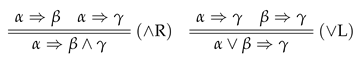
The sequent calculus $\mathsf{GRBL}$ consists of the following axiom and rules:

(1) 

Axiom:

$$\left(\mathrm{Id}\right)\alpha \Rightarrow \alpha$$

(2) 

$$\frac{\mathsf{\Gamma }[\top ]\Rightarrow \alpha }{\mathsf{\Gamma }\left[\mathsf{\Delta }\right]\Rightarrow \alpha }(\top )\frac{\mathsf{\Delta }\Rightarrow \perp }{\mathsf{\Gamma }\left[\mathsf{\Delta }\right]\Rightarrow \alpha }(\perp )$$

$$\frac{\mathsf{\Delta }\Rightarrow \alpha \mathsf{\Gamma }\left[\beta \right]\Rightarrow \gamma }{\mathsf{\Gamma }[\mathsf{\Delta }\odot (\alpha \to \beta \left)\right]\Rightarrow \gamma }(\to \mathrm{L})\frac{\alpha \odot \mathsf{\Gamma }\Rightarrow \beta }{\mathsf{\Gamma }\Rightarrow \alpha \to \beta }(\to \mathrm{R})$$

$$\frac{\mathsf{\Gamma }\left[\alpha \right]\Rightarrow \gamma \mathsf{\Delta }\Rightarrow \beta }{\mathsf{\Gamma }\left[\right(\alpha \leftarrow \beta )\odot \mathsf{\Delta }]\Rightarrow \gamma }(\leftarrow \mathrm{L})\frac{\mathsf{\Gamma }\odot \beta \Rightarrow \alpha }{\mathsf{\Gamma }\Rightarrow \alpha \leftarrow \beta }(\leftarrow \mathrm{R})$$

$$\frac{\mathsf{\Gamma }[\alpha \odot \beta ]\Rightarrow \gamma }{\mathsf{\Gamma }[\alpha •\beta ]\Rightarrow \gamma }(•\mathrm{L})\frac{\mathsf{\Gamma }\Rightarrow \alpha \mathsf{\Delta }\Rightarrow \beta }{\mathsf{\Gamma }\odot \mathsf{\Delta }\Rightarrow \alpha •\beta }(•\mathrm{R})$$

$$\frac{\mathsf{\Gamma }\left[\alpha \beta \right]\Rightarrow \gamma }{\mathsf{\Gamma }[\alpha \wedge \beta ]\Rightarrow \gamma }(\wedge \mathrm{L})\frac{\mathsf{\Gamma }\Rightarrow \alpha \mathsf{\Delta }\Rightarrow \beta }{\mathsf{\Gamma }\mathsf{\Delta }\Rightarrow \alpha \wedge \beta }(\wedge \mathrm{R})$$

$$\frac{\mathsf{\Gamma }\left[\alpha \right]\Rightarrow \gamma \mathsf{\Gamma }\left[\beta \right]\Rightarrow \gamma }{\mathsf{\Gamma }[\alpha \vee \beta ]\Rightarrow \gamma }(\vee \mathrm{L})\frac{\mathsf{\Gamma }\Rightarrow {\alpha }_i}{\mathsf{\Gamma }\Rightarrow {\alpha }_1\vee {\alpha }_2}(\vee \mathrm{R})(i=1,2)$$

The RBL-structure Γ in $(\to$$\mathrm{R})$ and $(\leftarrow$$\mathrm{R})$ is required to be nonempty. The formula with a connective in a logical rule is called principal.

(3) 

$$\frac{\mathsf{\Gamma }\left[\mathsf{\Delta }\overline{)\wedge }\mathsf{\Delta }\right]\Rightarrow \alpha }{\mathsf{\Gamma }\left[\mathsf{\Delta }\right]\Rightarrow \alpha }\left(\overline{)\wedge }\mathrm{C}\right)\frac{\mathsf{\Gamma }\left[\right(\mathsf{\Lambda }\odot \mathsf{\Delta })\odot \mathsf{\Delta }]\Rightarrow \alpha }{\mathsf{\Gamma }[\mathsf{\Lambda }\odot \mathsf{\Delta }]\Rightarrow \alpha }(\odot \mathrm{C})$$

$$\frac{\mathsf{\Gamma }\left[\mathsf{\Delta }\overline{)\wedge }\mathsf{\Lambda }\right]\Rightarrow \alpha }{\mathsf{\Gamma }\left[\mathsf{\Lambda }\overline{)\wedge }\mathsf{\Delta }\right]\Rightarrow \alpha }\left(\overline{)\wedge }\mathrm{E}\right)\frac{\mathsf{\Gamma }\left[{\mathsf{\Delta }}_i\right]\Rightarrow \alpha }{\mathsf{\Gamma }[{\mathsf{\Delta }}_1\ast {\mathsf{\Delta }}_2]\Rightarrow \alpha }\left(\mathrm{W}\right)(\ast \in \{\overline{)\wedge },\odot \})(i=1,2)$$

                       

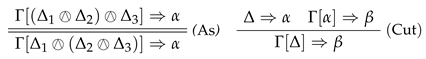
The RBL-structure Λ in $(\odot \mathrm{C})$ is nonempty. The double line in the rule $\left(\mathrm{As}\right)$ indicates that the premiss and the conclusion can be derived from each other.

A derivation in $\mathsf{GRBL}$ is a finite tree of sequents in which each node is either an instance of $\left(\mathrm{Id}\right)$ or obtained from a child node(s) by a rule. The height of a derivation is the greatest number of successive applications of rules. An instance of $\left(\mathrm{Id}\right)$ has height 0. We use $\mathsf{GRBL}⊢\mathsf{\Gamma }\Rightarrow \alpha$ for that the sequent $\mathsf{\Gamma }\Rightarrow \alpha$ is derivable in $\mathsf{GRBL}$.

 

Remark 3.

By the definition of $\mathsf{GRBL}$, if $\mathsf{GRBL}⊢\mathsf{\Gamma }\Rightarrow \alpha$, then Γ must be nonempty. Hence $\Rightarrow \top$ is not derivable. However $\top \Rightarrow \top$ is an instance of $\left(\mathrm{Id}\right)$ in $\mathsf{GRBL}$. Moreover, the following sequent rule is admissible in $\mathsf{GRBL}$:

$$\frac{\mathsf{\Gamma }[({\mathsf{\Delta }}_1\odot {\mathsf{\Delta }}_2)\odot {\mathsf{\Delta }}_3]\Rightarrow \alpha }{\mathsf{\Gamma }[{\mathsf{\Delta }}_1\odot ({\mathsf{\Delta }}_2\odot {\mathsf{\Delta }}_3)]\Rightarrow \alpha }(\odot {\mathrm{A}}_1)$$

This rule is half of the associativity.

Theorem 8.

For every RBL-sequent $\mathsf{\Gamma }\Rightarrow \alpha$, $\mathsf{SRBL}⊢\mu \left(\mathsf{\Gamma }\right)\Rightarrow \alpha$ if and only if $\mathsf{GRBL}⊢\mathsf{\Gamma }\Rightarrow \alpha$.

Proof. 

We give an outline of the proof. For the ‘only if’ part, assume $\mathsf{SRBL}⊢\mu \left(\mathsf{\Gamma }\right)\Rightarrow \alpha$. It is easy to show that every basic sequent provable in $\mathsf{SRBL}$ is derivable in $\mathsf{GRBL}$. Furthermore, $\mathsf{GRBL}⊢\mu \left(\mathsf{\Gamma }\right)\Rightarrow \alpha$. By the definition of $\mu$, $\mathsf{GRBL}⊢\mathsf{\Gamma }\Rightarrow \alpha$. For the ‘if’ part, assume $\mathsf{SRBL}\cancel{⊢}\mu \left(\mathsf{\Gamma }\right)\Rightarrow \alpha$. By the completeness of $\mathsf{SRBL}$, there exists an RBA $\mathbb{A}$ such that $\mathbb{A}\cancel{\vDash }\mu \left(\mathsf{\Gamma }\right)\Rightarrow \alpha$. Furthermore,, $\mathbb{A}\cancel{\vDash }\mathsf{\Gamma }\Rightarrow \alpha$. Clearly $\mathsf{GRBL}$ is sound with respect to $\mathsf{RBA}$. Hence $\mathsf{GRBL}\cancel{⊢}\mathsf{\Gamma }\Rightarrow \alpha$. □

5.2. Mix Elimination, Subformula Property and Decidability

We introduce the sequent calculus ${\mathsf{G}}_{\mathsf{RBL}}^{\mathsf{m}}$ which is obtained from $\mathsf{GRBL}$ by replacing the (Cut) rule with the following mix rule:

$$\frac{\mathsf{\Delta }\Rightarrow \alpha \mathsf{\Gamma }\left[\alpha \right]\dots \left[\alpha \right]\Rightarrow \beta }{\mathsf{\Gamma }\left[\mathsf{\Delta }\right]\dots \left[\mathsf{\Delta }\right]\Rightarrow \beta }\left(\mathrm{Mix}\right)$$

where $\mathsf{\Gamma }\left[\alpha \right]\dots \left[\alpha \right]$ denotes the formula structure containing at least one occurrence of $\alpha$, and $\mathsf{\Gamma }\left[\mathsf{\Delta }\right]\dots \left[\mathsf{\Delta }\right]$ denotes the formula structure obtained by replacing at least one occurrence of $\alpha$ in $\mathsf{\Gamma }\left[\alpha \right]\dots \left[\alpha \right]$ by the formula structure $\mathsf{\Delta }$. The formula $\alpha$ in the rule (Mix) is called the mixed formula. Note that (Cut) in $\mathsf{GRBL}$ is a special case of (Mix), and (Mix) is the finitely many times of application of (Cut). Hence $\mathsf{GRBL}$ is equivalent to ${\mathsf{G}}_{\mathsf{RBL}}^{\mathsf{m}}$.

Theorem 9

(Mix-elimination). Every RBL-sequent that is derivable in ${\mathsf{G}}_{\mathsf{RBL}}^{\mathsf{m}}$ admits a derivation without using $\left(\mathrm{Mix}\right)$.

Proof. 

Let an application of (Mix) in a derivation of a sequent in ${\mathsf{G}}_{\mathsf{RBL}}^{\mathsf{m}}$ be

$$\frac{\mathsf{\Delta }\Rightarrow \alpha \mathsf{\Gamma }\left[\alpha \right]\dots \left[\alpha \right]\Rightarrow \beta }{\mathsf{\Gamma }\left[\mathsf{\Delta }\right]\dots \left[\mathsf{\Delta }\right]\Rightarrow \beta }\left(\mathrm{Mix}\right)$$

where derivations of both premisses do not use (Mix). We prove the mix-elimination by simultaneous induction on (I) the complexity of the mixed formula $\alpha$, (II) the height of a derivation of $\mathsf{\Gamma }\left[\alpha \right]\dots \left[\alpha \right]\Rightarrow \beta$, and (III) the height of a derivation of $\mathsf{\Delta }\Rightarrow \alpha$. Let $\mathsf{\Delta }\Rightarrow \alpha$ be obtained by $\left(R_1\right)$ and $\mathsf{\Gamma }\left[\alpha \right]\dots \left[\alpha \right]\Rightarrow \beta$ by $\left(R_2\right)$. If $\left(R_1\right)$ is $\left(\mathrm{Id}\right)$, then $\mathsf{\Delta }=\alpha$ and the conclusion $\mathsf{\Gamma }\left[\mathsf{\Delta }\right]\dots \left[\mathsf{\Delta }\right]\Rightarrow \beta$ is obtained by the right premiss of (Mix). If $\left(R_2\right)$ is $\left(\mathrm{Id}\right)$, then $\alpha =\beta$ and $\mathsf{\Gamma }\left[\mathsf{\Delta }\right]\dots \left[\mathsf{\Delta }\right]\Rightarrow \beta$ is $\mathsf{\Delta }\Rightarrow \beta$, which is the left premiss of (Mix). Assume $\left(R_1\right)$ is a structural rule, then we apply (Mix) to the premiss(es) and then apply the rule $\left(R_1\right)$. The case that $\left(R_2\right)$ is a structural rule is quite similar. Now, assume that neither $\left(R_1\right)$ nor $\left(R_2\right)$ is an instance of $\left(\mathrm{Id}\right)$ or a structural rule. We have the following cases:

Case 1. The mixed formula $\alpha$ is not principal in $\left(R_1\right)$. We have the following cases:

(1.1)

$\left(R_1\right)$ is $(\top )$. The derivation

$$\frac{\frac{\mathsf{\Lambda }[\top ]\Rightarrow \alpha }{\mathsf{\Lambda }\left[{\mathsf{\Delta }}^{\prime }\right]\Rightarrow \alpha }(\top )\mathsf{\Gamma }\left[\alpha \right]\dots \left[\alpha \right]\Rightarrow \beta }{\mathsf{\Gamma }\left[\mathsf{\Lambda }\left[{\mathsf{\Delta }}^{\prime }\right]\right]\dots \left[\mathsf{\Lambda }\left[{\mathsf{\Delta }}^{\prime }\right]\right]\Rightarrow \beta }\left(\mathrm{Mix}\right)$$

is transformed into

$$\frac{\mathsf{\Lambda }[\top ]\Rightarrow \alpha \mathsf{\Gamma }\left[\alpha \right]\dots \left[\alpha \right]\Rightarrow \beta }{\frac{\mathsf{\Gamma }\left[\mathsf{\Lambda }\right[\top \left]\right]\dots \left[\mathsf{\Lambda }\right[\top \left]\right]\Rightarrow \beta }{\mathsf{\Gamma }\left[\mathsf{\Lambda }\left[{\mathsf{\Delta }}^{\prime }\right]\right]\dots \left[\mathsf{\Lambda }\left[{\mathsf{\Delta }}^{\prime }\right]\right]\Rightarrow \beta }\left({\top }^{\ast }\right)}\left(\mathrm{Mix}\right)$$

where $\left({\top }^{\ast }\right)$ denotes finitely many applications of the rule $(\top )$.

(1.2)

$\left(R_1\right)$ is a left logical rule. Apply (Mix) to $\mathsf{\Gamma }\left[\alpha \right]\dots \left[\alpha \right]\Rightarrow \beta$ and the premiss(es) of $\left(R_1\right)$, and then apply $\left(R_1\right)$. For example, $\left(R_1\right)=(\to$$\mathrm{L})$. The derivation

$$\frac{\frac{{\mathsf{\Delta }}_1\Rightarrow \gamma {\mathsf{\Delta }}_2\left[\delta \right]\Rightarrow \alpha }{{\mathsf{\Delta }}_2[{\mathsf{\Delta }}_1\odot (\gamma \to \delta )]\Rightarrow \alpha }(\to \mathrm{L})\mathsf{\Gamma }\left[\alpha \right]\dots \left[\alpha \right]\Rightarrow \beta }{\mathsf{\Gamma }\left[{\mathsf{\Delta }}_2[{\mathsf{\Delta }}_1\odot (\gamma \to \delta )]\right]\dots \left[{\mathsf{\Delta }}_2[{\mathsf{\Delta }}_1\odot (\gamma \to \delta )]\right]\Rightarrow \beta }\left(\mathrm{Mix}\right)$$

is transformed into

$$\frac{{\mathsf{\Delta }}_1\Rightarrow \gamma \frac{{\mathsf{\Delta }}_2\left[\delta \right]\Rightarrow \alpha \mathsf{\Gamma }\left[\alpha \right]\dots \left[\alpha \right]\Rightarrow \beta }{\mathsf{\Gamma }\left[{\mathsf{\Delta }}_2\left[\delta \right]\right]\dots \left[{\mathsf{\Delta }}_2\left[\delta \right]\right]\Rightarrow \beta }\left(\mathrm{Mix}\right)}{\mathsf{\Gamma }\left[{\mathsf{\Delta }}_2[{\mathsf{\Delta }}_1\odot (\gamma \to \delta )]\right]\dots \left[{\mathsf{\Delta }}_2[{\mathsf{\Delta }}_1\odot (\gamma \to \delta )]\right]\Rightarrow \beta }(\to {\mathrm{L}}^{\ast })$$

where $(\to {\mathrm{L}}^{\ast })$ denotes finitely many applications of the rule $(\to \mathrm{L})$.

Case 2. The mixed formula $\alpha$ is principal only in $\left(R_1\right)$. Furthermore, we have the following cases according to $\left(R_2\right)$:

(2.1)

$\left(R_2\right)$ is a right logical rule. Apply (Mix) to $\mathsf{\Delta }\Rightarrow \alpha$ and the premiss(es) of $R_2$, and then apply $\left(R_2\right)$. For example, $\left(R_2\right)=(•\mathrm{R})$. The derivation

$$\frac{\mathsf{\Delta }\Rightarrow \alpha \frac{{\mathsf{\Gamma }}_1\left[\alpha \right]\dots \left[\alpha \right]\Rightarrow {\beta }_1{\mathsf{\Gamma }}_2\left[\alpha \right]\dots \left[\alpha \right]\Rightarrow {\beta }_2}{{\mathsf{\Gamma }}_1\left[\alpha \right]\dots \left[\alpha \right]\odot {\mathsf{\Gamma }}_2\left[\alpha \right]\dots \left[\alpha \right]\Rightarrow {\beta }_1•{\beta }_2}(•\mathrm{R})}{{\mathsf{\Gamma }}_1\left[\mathsf{\Delta }\right]\dots \left[\mathsf{\Delta }\right]\odot {\mathsf{\Gamma }}_2\left[\mathsf{\Delta }\right]\dots \left[\mathsf{\Delta }\right]\Rightarrow {\beta }_1•{\beta }_2}\left(\mathrm{Mix}\right)$$

is transformed into

$$\frac{\frac{\mathsf{\Delta }\Rightarrow \alpha {\mathsf{\Gamma }}_1\left[\alpha \right]\dots \left[\alpha \right]\Rightarrow {\beta }_1}{{\mathsf{\Gamma }}_1\left[\mathsf{\Delta }\right]\dots \left[\mathsf{\Delta }\right]\Rightarrow {\beta }_1}\left(\mathrm{Mix}\right)\frac{\mathsf{\Delta }\Rightarrow \alpha {\mathsf{\Gamma }}_2\left[\alpha \right]\dots \left[\alpha \right]\Rightarrow {\beta }_1}{{\mathsf{\Gamma }}_2\left[\mathsf{\Delta }\right]\dots \left[\mathsf{\Delta }\right]\Rightarrow {\beta }_2}\left(\mathrm{Mix}\right)}{{\mathsf{\Gamma }}_1\left[\alpha \right]\dots \left[\alpha \right]\odot {\mathsf{\Gamma }}_2\left[\alpha \right]\dots \left[\alpha \right]\Rightarrow {\beta }_1•{\beta }_2}(•\mathrm{R})$$

(2.2)

$\left(R_2\right)$ is a left logical rule. Since $\alpha$ is not principal in $\left(R_2\right)$, we apply (Mix) to $\mathsf{\Delta }\Rightarrow \alpha$ and the premiss(es) of $\left(R_2\right)$ and then apply $\left(R_2\right)$. For example, $\left(R_2\right)=(\to \mathrm{L})$. The derivation

$$\frac{\mathsf{\Delta }\Rightarrow \alpha \frac{{\mathsf{\Delta }}^{\prime }\left[\alpha \right]\dots \left[\alpha \right]\Rightarrow \gamma {\mathsf{\Gamma }}^{\prime }\left[\delta \right]\left[\alpha \right]\dots \left[\alpha \right]\Rightarrow \beta }{{\mathsf{\Gamma }}^{\prime }[{\mathsf{\Delta }}^{\prime }\left[\alpha \right]\dots \left[\alpha \right]\odot (\gamma \to \delta )]\left[\alpha \right]\dots \left[\alpha \right]\Rightarrow \beta }(\to \mathrm{L})}{{\mathsf{\Gamma }}^{\prime }[{\mathsf{\Delta }}^{\prime }\left[\mathsf{\Delta }\right]\dots \left[\mathsf{\Delta }\right]\odot (\gamma \to \delta )]\left[\mathsf{\Delta }\right]\dots \left[\mathsf{\Delta }\right]\Rightarrow \beta }\left(\mathrm{Mix}\right)$$

is transformed into

$$\frac{\frac{\mathsf{\Delta }\Rightarrow \alpha {\mathsf{\Delta }}^{\prime }\left[\alpha \right]\dots \left[\alpha \right]\Rightarrow \gamma }{{\mathsf{\Delta }}^{\prime }\left[\mathsf{\Delta }\right]\dots \left[\mathsf{\Delta }\right]\Rightarrow \gamma }\left(\mathrm{Mix}\right)\frac{\mathsf{\Delta }\Rightarrow \alpha {\mathsf{\Gamma }}^{\prime }\left[\delta \right]\left[\alpha \right]\dots \left[\alpha \right]\Rightarrow \beta }{{\mathsf{\Gamma }}^{\prime }\left[\delta \right]\left[\mathsf{\Delta }\right]\dots \left[\mathsf{\Delta }\right]\Rightarrow \beta }\left(\mathrm{Mix}\right)}{{\mathsf{\Gamma }}^{\prime }[{\mathsf{\Delta }}^{\prime }\left[\mathsf{\Delta }\right]\dots \left[\mathsf{\Delta }\right]\odot (\gamma \to \delta )]\left[\mathsf{\Delta }\right]\dots \left[\mathsf{\Delta }\right]\Rightarrow \beta }(\to \mathrm{L})$$

Case 3. The mixed formula $\alpha$ is principal both in $\left(R_1\right)$ and $\left(R_2\right)$. We have the following cases according to the complexity of $\alpha$:

(3.1)

$\alpha ={\alpha }_1•{\alpha }_2$. Let the derivation end with

$$\frac{\frac{{\mathsf{\Delta }}_1\Rightarrow {\alpha }_1{\mathsf{\Delta }}_2\Rightarrow {\alpha }_2}{{\mathsf{\Delta }}_1\odot {\mathsf{\Delta }}_2\Rightarrow {\alpha }_1•{\alpha }_2}(•\mathrm{R})\frac{\mathsf{\Gamma }[{\alpha }_1\odot {\alpha }_2]\left[\alpha \right]\dots \left[\alpha \right]\Rightarrow \beta }{\mathsf{\Gamma }[{\alpha }_1•{\alpha }_2]\left[\alpha \right]\dots \left[\alpha \right]\Rightarrow \beta }(•\mathrm{L})}{\mathsf{\Gamma }[{\mathsf{\Delta }}_1\odot {\mathsf{\Delta }}_2]\dots [{\mathsf{\Delta }}_1\odot {\mathsf{\Delta }}_2]\Rightarrow \beta }\left(\mathrm{Mix}\right)$$

By the induction hypothesis, we have the following derivation:

$$\frac{{\mathsf{\Delta }}_1\odot {\mathsf{\Delta }}_2\Rightarrow {\alpha }_1•{\alpha }_2\mathsf{\Gamma }[{\alpha }_1\odot {\alpha }_2]\left[\alpha \right]\dots \left[\alpha \right]\Rightarrow \beta }{\mathsf{\Gamma }[{\alpha }_1\odot {\alpha }_2][{\mathsf{\Delta }}_1\odot {\mathsf{\Delta }}_2]\dots [{\mathsf{\Delta }}_1\odot {\mathsf{\Delta }}_2]\Rightarrow \beta }\left(\mathrm{Mix}\right)$$

By induction hypothesis on ${\alpha }_1$ and ${\alpha }_2$, we have the following derivation:

$$\frac{{\mathsf{\Delta }}_2\Rightarrow {\alpha }_2\frac{{\mathsf{\Delta }}_1\Rightarrow {\alpha }_1\mathsf{\Gamma }[{\alpha }_1\odot {\alpha }_2][{\mathsf{\Delta }}_1\odot {\mathsf{\Delta }}_2]\dots [{\mathsf{\Delta }}_1\odot {\mathsf{\Delta }}_2]\Rightarrow \beta }{\mathsf{\Gamma }[{\mathsf{\Delta }}_1\odot {\alpha }_2][{\mathsf{\Delta }}_1\odot {\mathsf{\Delta }}_2]\dots [{\mathsf{\Delta }}_1\odot {\mathsf{\Delta }}_2]\Rightarrow \beta }\left(\mathrm{Mix}\right)}{\mathsf{\Gamma }[{\mathsf{\Delta }}_1\odot {\mathsf{\Delta }}_2]\dots [{\mathsf{\Delta }}_1\odot {\mathsf{\Delta }}_2]\Rightarrow \beta }\left(\mathrm{Mix}\right)$$

(3.2)

$\alpha ={\alpha }_1\to {\alpha }_2$ or $\alpha ={\alpha }_1\leftarrow {\alpha }_2$. These two cases are similar. Here we show only the case $\alpha ={\alpha }_1\to {\alpha }_2$. Let the derivation end with

$$\frac{\frac{{\alpha }_1\odot \mathsf{\Delta }\Rightarrow {\alpha }_2}{\mathsf{\Delta }\Rightarrow {\alpha }_1\to {\alpha }_2}(\to \mathrm{R})\frac{{\mathsf{\Delta }}^{\prime }\left[\alpha \right]\dots \left[\alpha \right]\Rightarrow {\alpha }_1{\mathsf{\Gamma }}^{\prime }\left[{\alpha }_2\right]\left[\alpha \right]\dots \left[\alpha \right]\Rightarrow \beta }{{\mathsf{\Gamma }}^{\prime }[{\mathsf{\Delta }}^{\prime }\left[\alpha \right]\dots \left[\alpha \right]\odot ({\alpha }_1\to {\alpha }_2)]\left[\alpha \right]\dots \left[\alpha \right]\Rightarrow \beta }(\to \mathrm{L})}{{\mathsf{\Gamma }}^{\prime }[{\mathsf{\Delta }}^{\prime }\left[\mathsf{\Delta }\right]\dots \left[\mathsf{\Delta }\right]\odot \mathsf{\Delta }]\left[\mathsf{\Delta }\right]\dots \left[\mathsf{\Delta }\right]\Rightarrow \beta }\left(\mathrm{Mix}\right)$$

By induction hypothesis, we have the following derivations:

$$\frac{\mathsf{\Delta }\Rightarrow {\alpha }_1\to {\alpha }_2{\mathsf{\Delta }}^{\prime }\left[\alpha \right]\dots \left[\alpha \right]\Rightarrow {\alpha }_1}{{\mathsf{\Delta }}^{\prime }\left[\mathsf{\Delta }\right]\dots \left[\mathsf{\Delta }\right]\Rightarrow {\alpha }_1}\left(\mathrm{Mix}\right)$$

and

$$\frac{\mathsf{\Delta }\Rightarrow {\alpha }_1\to {\alpha }_2{\mathsf{\Gamma }}^{\prime }\left[{\alpha }_2\right]\left[\alpha \right]\dots \left[\alpha \right]\Rightarrow \beta }{{\mathsf{\Gamma }}^{\prime }\left[{\alpha }_2\right]\left[\mathsf{\Delta }\right]\dots \left[\mathsf{\Delta }\right]\Rightarrow \beta }\left(\mathrm{Mix}\right)$$

By induction hypothesis on ${\alpha }_1$, we have

$$\frac{{\mathsf{\Delta }}^{\prime }\left[\mathsf{\Delta }\right]\dots \left[\mathsf{\Delta }\right]\Rightarrow {\alpha }_1{\alpha }_1\odot \mathsf{\Delta }\Rightarrow {\alpha }_2}{{\mathsf{\Delta }}^{\prime }\left[\mathsf{\Delta }\right]\dots \left[\mathsf{\Delta }\right]\odot \mathsf{\Delta }\Rightarrow {\alpha }_2}\left(\mathrm{Mix}\right)$$

By induction hypothesis on ${\alpha }_2$, we have

$$\frac{{\mathsf{\Delta }}^{\prime }\left[\mathsf{\Delta }\right]\dots \left[\mathsf{\Delta }\right]\odot \mathsf{\Delta }\Rightarrow {\alpha }_2{\mathsf{\Gamma }}^{\prime }\left[{\alpha }_2\right]\left[\mathsf{\Delta }\right]\dots \left[\mathsf{\Delta }\right]\Rightarrow \beta }{{\mathsf{\Gamma }}^{\prime }[{\mathsf{\Delta }}^{\prime }\left[\mathsf{\Delta }\right]\dots \left[\mathsf{\Delta }\right]\odot \mathsf{\Delta }]\left[\mathsf{\Delta }\right]\dots \left[\mathsf{\Delta }\right]\Rightarrow \beta }\left(\mathrm{Mix}\right)$$

(3.3)

$\alpha ={\alpha }_1\wedge {\alpha }_2$ or $\alpha ={\alpha }_1\vee {\alpha }_2$. These two cases are similar. Here we show only the case $\alpha ={\alpha }_1\wedge {\alpha }_2$. Let the derivation end with

$$\frac{\frac{\mathsf{\Delta }\Rightarrow {\alpha }_1\mathsf{\Delta }\Rightarrow {\alpha }_2}{\mathsf{\Delta }\Rightarrow {\alpha }_1\wedge {\alpha }_2}(\wedge \mathrm{R})\frac{\mathsf{\Gamma }\left[{\alpha }_1\overline{)\wedge }{\alpha }_2\right]\left[\alpha \right]\dots \left[\alpha \right]\Rightarrow \beta }{\mathsf{\Gamma }[{\alpha }_1\wedge {\alpha }_2]\left[\alpha \right]\dots \left[\alpha \right]\Rightarrow \beta }(•\mathrm{L})}{\mathsf{\Gamma }\left[\mathsf{\Delta }\right]\dots \left[\mathsf{\Delta }\right]\Rightarrow \beta }\left(\mathrm{Mix}\right)$$

By induction hypothesis, we have the following derivation:

$$\frac{\mathsf{\Delta }\Rightarrow {\alpha }_1\wedge {\alpha }_2\mathsf{\Gamma }\left[{\alpha }_1\overline{)\wedge }{\alpha }_2\right]\left[\alpha \right]\dots \left[\alpha \right]\Rightarrow \beta }{\mathsf{\Gamma }\left[{\alpha }_1\overline{)\wedge }{\alpha }_2\right]\left[\mathsf{\Delta }\right]\dots \left[\mathsf{\Delta }\right]\Rightarrow \beta }\left(\mathrm{Mix}\right)$$

By the induction hypothesis on ${\alpha }_1$ and ${\alpha }_2$, we have

$$\frac{\mathsf{\Delta }\Rightarrow {\alpha }_1\frac{\mathsf{\Delta }\Rightarrow {\alpha }_1\mathsf{\Gamma }\left[{\alpha }_1\overline{)\wedge }{\alpha }_2\right]\left[\mathsf{\Delta }\right]\dots \left[\mathsf{\Delta }\right]\Rightarrow \beta }{\mathsf{\Gamma }\left[\mathsf{\Delta }\overline{)\wedge }{\alpha }_2\right]\left[\mathsf{\Delta }\right]\dots \left[\mathsf{\Delta }\right]\Rightarrow \beta }\left(\mathrm{Mix}\right)}{\frac{\mathsf{\Gamma }\left[\mathsf{\Delta }\overline{)\wedge }\mathsf{\Delta }\right]\left[\mathsf{\Delta }\right]\dots \left[\mathsf{\Delta }\right]\Rightarrow \beta }{\mathsf{\Gamma }\left[\mathsf{\Delta }\right]\dots \left[\mathsf{\Delta }\right]\Rightarrow \beta }\left(\overline{)\wedge }\mathrm{C}\right)}\left(\mathrm{Mix}\right)$$

This completes the proof. □

Corollary 3

(Subformula Property). If $\mathsf{GRBL}⊢\mathsf{\Gamma }\Rightarrow \alpha$, then there exists a derivation of $\mathsf{\Gamma }\Rightarrow \alpha$ in $\mathsf{GRBL}$ in which every formula is a subformula of formulas in $\mathsf{\Gamma }\cup \{\alpha ,\top ,\perp \}$.

Theorem 10

(Disjunction Property). For all RBL-formulas α and β, if $\mathsf{GRBL}⊢\top \Rightarrow \alpha \vee \beta$, then $\mathsf{GRBL}⊢\top \Rightarrow \alpha$ or $\mathsf{GRBL}⊢\top \Rightarrow \beta$.

 

Proof. 

Assume $\mathsf{GRBL}⊢\top \Rightarrow \alpha \vee \beta$. Furthermore, ${\mathsf{G}}_{\mathsf{RBL}}^{\mathsf{m}}⊢\top \Rightarrow \alpha \vee \beta$. By Theorem 9, the last rule of a mix-free derivation of $\top \Rightarrow \alpha \vee \beta$ can be only $(\vee \mathrm{R})$ or ($\overline{)\wedge }\mathrm{C}$). Assume the last application of $(\vee \mathrm{R})$ is $\top \overline{)\wedge }\dots \overline{)\wedge }\top \Rightarrow \alpha \vee \beta$. Furthermore, the premiss of $(\vee \mathrm{R})$ is $\top \overline{)\wedge }\dots \overline{)\wedge }\top \Rightarrow \alpha$ or $\top \dots \top \Rightarrow \beta$. By ($\overline{)\wedge }\mathrm{C}$), $\mathsf{GRBL}⊢\top \Rightarrow \alpha$ or $\mathsf{GRBL}⊢\top \Rightarrow \beta$. □

If rules for • and ← are dropped from $\mathsf{GRBL}$, we get the sequent calculus $\mathsf{GBPL}$ with two structure operators $\overline{)\wedge }$ and ⊙. Thus, $\mathsf{GBPL}$ can be taken as a sequent calculus for basic propositional logic. We have the following result:

Theorem 11.

For every basic BPL-sequent $\alpha \Rightarrow \beta$, $\mathsf{SBCA}⊢\alpha \Rightarrow \beta$ if and only if $\mathsf{GBPL}⊢\alpha \Rightarrow \beta$.

 

Proof. 

Let $\alpha \Rightarrow \beta$ be a basic BPL-sequent. By Theorem 7, $\mathsf{SBCA}⊢\alpha \Rightarrow \beta$ if and only if $\mathsf{SRBL}⊢\alpha \Rightarrow \beta$. Clearly $\mathsf{SRBL}⊢\alpha \Rightarrow \beta$ if and only if $\mathsf{GRBL}⊢\alpha \Rightarrow \beta$. By the subformula property of $\mathsf{GRBL}$, $\mathsf{GRBL}⊢\alpha \Rightarrow \beta$ if and only if $\mathsf{GBPL}⊢\alpha \Rightarrow \beta$. □

Finally, we consider the consequence relations of sequent calculi $\mathsf{GRBL}$ and $\mathsf{GBPL}$. A sequent $\mathsf{\Gamma }\Rightarrow \alpha$ is called a consequence of a finite set of sequents $\mathsf{\Phi }$ in $\mathsf{GRBL}$ (notation: $\mathsf{\Phi }{⊢}_{\mathsf{GRBL}}\mathsf{\Gamma }\Rightarrow \alpha$) if there exists a derivation of $\mathsf{\Gamma }\Rightarrow \alpha$ in $\mathsf{GRBL}$ from sequents in $\mathsf{\Phi }$. The consequence relation of $\mathsf{GBPL}$ is defined similarly. We have shown that $\mathsf{RBA}$ has the FEP (Theorem 5). This property implies the universal finite model property (cf. Section 3), which yields the SFMP (cf. e.g., ([19], Chapter 6). It follows that $\mathsf{GRBL}$ has the strong finite model property (SFMP). That is, for every finite set of sequents $\mathsf{\Phi }$, if $\mathsf{\Phi }{\cancel{⊢}}_{\mathsf{GRBL}}\mathsf{\Gamma }\Rightarrow \alpha$, then there exists a finite RBA model $\mathbb{M}=(\mathbb{A},\mu )$ such that all sequents in $\mathsf{\Phi }$ are true but $\mathsf{\Gamma }\Rightarrow \alpha$ is not true in $\mathbb{M}$. This result follows immediately from the finite embeddability property of $\mathsf{RBA}$.

Theorem 12.

The consequence relations of $\mathsf{GRBL}$ and $\mathsf{GBPL}$ are decidable.

 

Proof. 

By the FEP of $\mathsf{RBA}$, we get the SFMP of $\mathsf{GRBL}$ and so the SFMP of $\mathsf{GBPL}$. Thus, consequence relations of $\mathsf{GRBL}$ and $\mathsf{GBPL}$ are decidable. □

6. Concluding Remarks

The present paper makes several contributions to the study of subintuitionistic logics. First, we introduce residuated basic algebras and show the finite embeddability property. Second, the residuated basic logic is shown to be a conservative extension of basic propositional logic. Third, we introduce a cut-free sequent calculus $\mathsf{GBPL}$ for residuated basic algebras. Finally, the consequence relation of $\mathsf{GRBL}$ is decidable.

Residuation often appears in algebraic structures, and residuated logics have been developed. Lambek calculi are typical systems for some residuated algebras. The residuated basic logic given in the present paper is obtained by introducing the binary operator • such that the implication in basic propositional logic is one of the right residuals. There are some relevant results in the literature. For example, a logic for residuated paritially ordered sets with a top was developed in e.g., [28]. In the setting of fuzzy logic (cf. e.g., [29]), residuated fuzzy logics arising from continuous t-norms without non-trivial zero divisors and extended with an involutive negation are developed in [30]. Hájeck’s basic logic is quite different from Visser’s basic propositional logic since the latter was developed from the study of formal provability. The workings of residuated basic logic in the study of provability need further exploration.

There are some interesting problems for future work. It is already known that intuitionistic logic is embedded into basic propositional logic by a bounded translation [31]. Using the sequent calculus $\mathsf{G}\mathsf{4}\mathsf{ip}$ for intuitionistic logic (cf. [32]) and $\mathsf{GRBL}$ for residuated basic logic, we could give a purely proof-theoretic proof of this result. Embedding results of this kind could be explored in an extended setting. For example, the embedding of propositional logics into modal logics could be explored by proof-theoretic methods. We can also consider extending the approach given in this paper to more extensions of basic propositional logic. The general question is to determine subintuitionistic propositional logics, which can be formalized as analytic Gentzen-style sequent calculi. Using such sequent calculi, we may obtain the logical properties of these logics.

References

- Celani, S.; Jansana, R. A closer look at some subintuitionistic logics. Notre Dame J. Form. Log. 2003, 42, 225–255. [Google Scholar] [CrossRef]
- Restall, G. Subintuitionistic logics. Notre Dame J. Form. Log. 1994, 35, 116–129. [Google Scholar] [CrossRef]
- Visser, A. A propositional logic with explicit fixed points. Stud. Log. 1981, 40, 155–175. [Google Scholar] [CrossRef]
- Chagrov, A.; Zakharyaschev, M. Modal Logic; Clarendon Press: Oxford, UK, 1997. [Google Scholar]
- Corsi, G. Weak logics with strict implication. Zeitschr. F. Math. Logik Grundlagen D. Math. 1987, 33, 389–406. [Google Scholar] [CrossRef]
- Suzuki, Y.; Wolter, F.; Zakharyaschev, M. Speaking about transitive frames in propositional languages. J. Log. Lang. Inf. 1998, 7, 317–339. [Google Scholar] [CrossRef]
- Ruitenburg, W. Constructive logics and the paradoxes. Rev. Mod. Log. 1991, 1, 271–301. [Google Scholar]
- Gentzen, G. Die widerspruchsfreiheit der reinen zahlentheorie. Math. Ann. 1936, 112, 493–565. [Google Scholar] [CrossRef]
- Ardeshir, M.; Ruitenburg, W. Basic propositional calculus I. Math. Log. Q. 1998, 44, 317–343. [Google Scholar] [CrossRef]
- Ardeshir, M.; Ruitenburg, W. Basic propositional calculus II. Interpolation. Arch. Math. Log. 2001, 40, 349–364. [Google Scholar] [CrossRef]
- Ardeshir, M. Aspects of Basic Logic. Ph.D. Thesis, Department of Mathematics, Marquette University, Milwaukee, WI, USA, 1995. [Google Scholar]
- Celani, S.; Jansana, R. Bounded distributive lattices with strict implication. Math. Log. Q. 2005, 51, 219–246. [Google Scholar] [CrossRef]
- Suzuki, Y.; Ono, H. Hilbert Style Proof System for BPL; Technical Report IS-RR-97-0040F 1(8); School of Information Science, Japan Advanced Institute of Science and Technology: Ishikawa, Japan, 1997. [Google Scholar]
- Aghaei, M.; Ardeshir, M. Gentzen-style axiomatizations for some conservative extensions of basic propositional logic. Stud. Log. 2001, 68, 263–285. [Google Scholar] [CrossRef]
- Ishii, K. Proof Theoretical Investigations for Visser’s Logics, Classical Logic and the First-Order Arithmetic. Ph.D. Thesis, Japan Advanced Institute of Science and Technology, Ishikawa, Japan, 2002. [Google Scholar]
- Ishii, K.; Kashima, R.; Kikuchi, K. Sequent calculi for Visser’s propositional logics. Notre Dame J. Form. Log. 2001, 42, 1–22. [Google Scholar] [CrossRef]
- Kikuchi, K.; Sasaki, K. A cut-free Gentzen formulation of basic propositional calculus. J. Log. Lang. Inf. 2003, 12, 213–225. [Google Scholar] [CrossRef]
- Buszkowski, W. Lambek calculus and substructural logics. Linguist. Anal. 2010, 36, 15–48. [Google Scholar]
- Galatos, N.; Jipsen, P.; Kowalski, T.; Ono, H. Residuated Lattices: An Algebraic Glimpse at Substructural Logics; Elsevier: Amsterdam, The Netherlands, 2007. [Google Scholar]
- Ono, H. Substructural logics and residuated lattices–an introduction. In Trends in Logic: 50 Years of Studia Logica; Hendricks, V.F., Ed.; Springer: Berlin/Heidelberg, Germany, 2003; pp. 177–212. [Google Scholar]
- Restall, G. Relevant and substructural logics. In Logic and the Modalities in the Twentieth Century; Gabbay, D., Woods, J., Eds.; Elsevier: Amsterdam, The Netherlands, 2006; Volume 7, pp. 289–398. [Google Scholar]
- Buszkowski, W.; Farulewski, M. Nonassociative Lambek calculus with additives and context-free languages. In Languages: From Formal to Natural, LNCS 5533; Springer: Berlin/Heidelberg, Germany, 2009; pp. 45–58. [Google Scholar]
- Lambek, J. On the calculus of syntactic types. Struct. Lang. Its Math. Asp. 1961, 12, 166–178. [Google Scholar]
- Galatos, N.; Ono, H. Cut elimination and strong separation for substructural logics: An algebraic approach. Ann. Pure Appl. Log. 2010, 161, 1097–1133. [Google Scholar] [CrossRef]
- Lambek, J. The mathematics of sentence structure. Am. Math. Mon. 1958, 65, 154–170. [Google Scholar] [CrossRef]
- Haniková, Z.; Horčík, R. The finite embeddability property for residuated groupoids. Algebra Univ. 2014, 72, 1–13. [Google Scholar] [CrossRef]
- Restall, G. On Logics without Contraction. Ph.D. Thesis, Department of Philosophy, University of Queensland, Woolloongabba, Australia, 1994. [Google Scholar]
- Morsi, N.N. A small set of axioms for residuated logic. Inf. Sci. 2005, 175, 85–96. [Google Scholar] [CrossRef]
- Hájek, P. Metamathematics of Fuzzy Logic; Springer: Dordrecht, The Netherlands, 1998. [Google Scholar]
- Esteva, F.; Godo, L.; Hájeck, P.; Navara, M. Residuated fuzzy logics with an involutive negation. Arch. Math. Log. 2000, 39, 103–124. [Google Scholar] [CrossRef]
- Aghaei, M.; Ardeshir, M. A bounded translation of intuitionistic propositional logic into basic propositional logic. Math. Log. Q. 2000, 46, 199–206. [Google Scholar] [CrossRef]
- Dyckhoff, R. Contraction-free sequent calculi for intuitionistic logic. J. Symb. Log. 1992, 57, 795–807. [Google Scholar] [CrossRef]
Disclaimer/Publisher’s Note: The statements, opinions and data contained in all publications are solely those of the individual author(s) and contributor(s) and not of MDPI and/or the editor(s). MDPI and/or the editor(s) disclaim responsibility for any injury to people or property resulting from any ideas, methods, instructions or products referred to in the content. |
© 2023 by the authors. Licensee MDPI, Basel, Switzerland. This article is an open access article distributed under the terms and conditions of the Creative Commons Attribution (CC BY) license (https://creativecommons.org/licenses/by/4.0/).