Complete Study of an Original Power-Exponential Transformation Approach for Generalizing Probability Distributions

Abstract

In this paper, we propose a flexible and general family of distributions based on an original power-exponential transformation approach. We call it the modified generalized-G (MGG) family. The elegance and significance of this family lie in the ability to modify the standard distributions by changing their functional forms without adding new parameters, by compounding two distributions, or by adding one or two shape parameters. The aim of this modification is to provide flexible shapes for the corresponding probability functions. In particular, the distributions of the MGG family can possess increasing, constant, decreasing, “unimodal”, or “bathtub-shaped“ hazard rate functions, which are ideal for fitting several real data sets encountered in applied fields. Some members of the MGG family are proposed for special distributions. Following that, the uniform distribution is chosen as a baseline distribution to yield the modified uniform (MU) distribution with the goal of efficiently modeling measures with bounded values. Some useful key properties of the MU distribution are determined. The estimation of the unknown parameters of the MU model is discussed using seven methods, and then, a simulation study is carried out to explore the performance of the estimates. The flexibility of this model is illustrated by the analysis of two real-life data sets. When compared to fair and well-known competitor models in contemporary literature, better-fitting results are obtained for the new model.

1. Introduction

Recently, some attempts have been made to introduce new families of distributions or generalize some of the presented distributions to provide high flexibility in the modeling of real phenomena based on data. They can involve special transformations that are possibly modulated by one or several parameters.

For example, Marshall and Olkin [1] proposed a method of adding an extra shape parameter to a given baseline distribution; the resulting distribution is known as the “expanded Marshall-Olkin (MO) distribution”. In order to fix the idea, let us present the mathematical foundations of the MO family. Consider an absolutely continuous baseline distribution depending on a generic parameter vector denoted by $\zeta$ and with support denoted by $\mathrm{D}\subseteq \mathbb{R}$, and the corresponding cumulative distribution function (cdf) and probability density function (pdf) denoted by $G\left(x;\zeta \right)$ and $g\left(x;\zeta \right)$, respectively. Then the survival function (sf) and pdf of the MO distribution are, respectively,

$$\overline{F}\left(x;\upsilon ,\zeta \right)=\frac{\upsilon G\left(x;\zeta \right)}{1-\left(1-\upsilon \right)\overline{G}\left(x;\zeta \right)},\upsilon >0,x\in \mathrm{D}$$

(1)

and

$$f\left(x;\upsilon ,\zeta \right)=\frac{\upsilon g\left(x;\zeta \right)}{{\left[1-\left(1-\upsilon \right)\overline{G}\left(x;\zeta \right)\right]}^2},$$

(2)

where $\upsilon$ is a shape parameter and $\overline{G}\left(x;\zeta \right)=1-G\left(x;\zeta \right)$. The MO family has inspired numerous studies for the modeling of various physical phenomena and has been extended in numerous ways. For more information, we refer the reader to the overview [2].

On the other hand, Eugene et al. [3] introduced a new family, which is generated from the beta distribution, called the beta-generated family. Its corresponding cdf takes the following form:

$$F\left(x;\upsilon ,\omega ,\zeta \right)=\frac{1}{B\left(\upsilon ,\omega \right)}{\int }_0^{G\left(x;\zeta \right)}{u}^{\upsilon -1}{\left(1-u\right)}^{\omega -1}du,\upsilon ,\omega >0,x\in \mathrm{D},$$

(3)

where $\upsilon$ and $\omega$ are two additional parameters whose rule is to increase the skewness and to vary tail weights, and $B\left(a,b\right)={\int }_0^1{t}^{a-1}{\left(1-t\right)}^{b-1}dt$ is the standard beta function. The pdf corresponding to Equation (3) is

$$f\left(x;\upsilon ,\omega ,\zeta \right)=\frac{1}{B\left(\upsilon ,\omega \right)}G{\left(x;\zeta \right)}^{\upsilon -1}\overline{G}{\left(x;\zeta \right)}^{\omega -1}g\left(x;\zeta \right).$$

(4)

For further developments on the beta family, we redirect the reader to [4]. As a remark, by taking $\omega =1$, the beta-generated family is reduced to the exponentiated-generated (ExG) family initiated in [5] and further discussed in detail in [6]. This special family plays a secondary role in our study.

Kumaraswamy’s work was also very inspiring in terms of proposing new modeling alternatives, starting with Reference [7]. The Kumaraswamy (K) distribution is a two-parameter distribution with support $\left(0,1\right)$ that has proven useful in many hydrological applications. Its cdf is defined by

$$F\left(x;\upsilon ,\omega \right)=1-{\left(1-x^{\upsilon }\right)}^{\omega },\upsilon ,\omega >0,x\in \left(0,1\right),$$

(5)

where $\upsilon$ and $\omega$ are two additional shape parameters. The corresponding pdf is

$$f\left(x;\upsilon ,\omega \right)=\upsilon \omega x^{\upsilon -1}{\left(1-x^{\upsilon }\right)}^{\omega -1}.$$

(6)

Based on the K distribution, Cordeiro and de Castro [8] introduced the K generated family. Its cdf takes the following form:

$$F\left(x;\upsilon ,\omega ,\zeta \right)=1-{\left(1-G{\left(x;\zeta \right)}^{\upsilon }\right)}^{\omega },\upsilon ,\omega >0,x\in \mathrm{D},$$

(7)

where $\upsilon$ and $\omega$ are two shape parameters. The corresponding pdf is

$$f\left(x;\upsilon ,\omega ,\zeta \right)=\upsilon \omega g\left(x;\zeta \right)G{\left(x;\zeta \right)}^{\upsilon -1}{\left(1-G{\left(x;\zeta \right)}^{\upsilon }\right)}^{\omega -1}.$$

(8)

By taking $\upsilon =1$, the K generated family is reduced to the type 2 exponentiated-generated (T2ExG) family, which will also play a secondary role in our study.

All the previous families and many other families in the statistical literature depend on adding one or more shape parameters to a baseline distribution in order to provide greater flexibility. This reason led the researchers to suggest alternative options that unify certain current families based on straightforward functional transformations (power, logarithmic, exponential, trigonometric, etc.). See, for example, the family based on a special poly-exponential transformation in [9] and the sine-generated family introduced in [10]. With this knowledge in mind, the findings of this paper are based on the following new theoretical approach: Let $H\left(x\right)$ be an sf of an absolutely continuous distribution with support $(0,1)$, and $K\left(x\right)$ be a decreasing continuous function such that $K\left(x\right)\in [0,1]$ and ${lim}_{x\to 0}K\left(x\right)=1$. Then, the following function is a valid cdf:

$$F\left(x\right)=1-H\left(x\right)K\left(x\right).$$

(9)

It is important to note that $K\left(x\right)$ is not necessarily a valid sf because we can have ${lim}_{x\to 1}K\left(x\right)\ne 0$, which allows for a wide range of functions. With the mathematical structure of Equation (9), various families can be created, but one interesting way is to choose $H\left(x\right)$ and $K\left(x\right)$ of different nature to enrich the functionalities of $F\left(x\right)$. In this paper, we follow this line by adopting an original power-exponential transformation approach: we chose $H\left(x\right)$ as the sf of the T2ExG family defined with a certain generic baseline distribution, and $K\left(x\right)$ as a decreasing exponential function compounds with a possible other baseline distribution. This created “unified family” is called the modified generalized-G (MGG) family. The new MGG family has the following significant and desirable ambitions in addition to its innovative construction:

• Thanks to its power-exponential transformation approach, the MGG family is capable of modifying the standard baseline distributions by changing their functional forms without adding any additional shape parameter.
• It can also provide more flexible generalized forms by adding one or two shape parameters.
• It can be considered as a compounding family. The MGG family can provide new generalized distributions by compounding two different baseline distributions.
• The special sub-distributions of the MGG family accommodates all important hazard rate (hr) shapes including bathtub, constant, upside down bathtub, increasing, decreasing–increasing–decreasing, and decreasing shapes. Hence, its special distributions can model different types of real-life data in many applied sciences.
• The MGG family is not generated based on the well-known baseline distributions similar to the MO, beta-generated, ExG, and K families.
• The special sub-distributions of the MGG family provide consistently better fits than its competing and baseline distributions.

All of these claims are supported in the paper with thorough investigations of theory and practice, as well as with the aid of graphics and quantitative information.

To be more specific, the paper is structured as follows: In Section 2, we define the MGG family and its important sub-families. In Section 3, we provide three special sub-distributions of the MGG family. In Section 4, the modified uniform (MU) distribution is studied with its analytical shapes. Section 5 provides some of its statistical properties. In Section 6, the parameters of the MU model are estimated using some classical estimation methods. A simulation study to compare the behavior of different estimates is presented in Section 7. In Section 8, the MU distribution is fitted to two real data sets. Finally, Section 9 offers some concluding remarks.

2. The New MGG Family

This section introduces and discusses the MGG family.

2.1. Definition

Assume that there are two absolutely continuous baseline distributions. The first one is defined on $\left(a,b\right)\subseteq \mathbb{R}$ with cdf $G_1\left(x;{\zeta }_1\right)$ and pdf $g_1\left(x;{\zeta }_1\right)$, while the second one is defined on $\left(a,c\right)\subseteq \mathbb{R}$ with cdf $G_2\left(x;{\zeta }_2\right)$ and pdf $g_2\left(x;{\zeta }_2\right)$, where $-\infty \le a<b<c\le \infty$. Based on Equation (9), the cdf of the MGG family can be written as follows:

$$F\left(x;\upsilon ,\omega ,{\zeta }_1,{\zeta }_2\right)=1-H\left(x;\upsilon ,{\zeta }_1\right)K\left(x;,\omega ,{\zeta }_2\right),\upsilon ,\omega >0,x\in \left(a,b\right),$$

(10)

where $H\left(x;\upsilon ,{\zeta }_1\right)={\overline{G}}_1{\left(x;{\zeta }_1\right)}^{\upsilon }$ and $K\left(x;,\omega ,{\zeta }_2\right)=e^{-G_2{\left(x;{\zeta }_2\right)}^{\omega }}$, and $\upsilon$ and $\omega$ are two shape parameters. Hence, this cdf can be expressed in a more direct manner as

$$F\left(x;\upsilon ,\omega ,{\zeta }_1,{\zeta }_2\right)=1-{\overline{G}}_1{\left(x;{\zeta }_1\right)}^{\upsilon }{e}^{-G_2{\left(x;{\zeta }_2\right)}^{\omega }}.$$

(11)

Here, $H\left(x;\upsilon ,{\zeta }_1\right)$ is the sf of the T2ExG family with the baseline cdf $G_1\left(x;{\zeta }_1\right)$ and parameter $\upsilon$, and $K\left(x;,\omega ,{\zeta }_2\right)$ is a decreasing exponential transformation of the cdf of the (standard) ExG family with the baseline cdf $G_2\left(x;{\zeta }_2\right)$ and parameter $\omega$.

There are some deep stochastic order connections between the MGG and T2ExG families, which are presented in the next proposition.

Proposition 1. 

 

• The following first order stochastic dominance property holds:

  $$F_{*}\left(x;\upsilon ,{\zeta }_1\right)\le F\left(x;\upsilon ,\omega ,{\zeta }_1,{\zeta }_2\right),$$

  (12)

  where $F_{*}\left(x;\upsilon ,{\zeta }_1\right)=1-{\overline{G}}_1{\left(x;{\zeta }_1\right)}^{\upsilon }$ is the cdf of the T2ExG family. Moreover, for x such that $G_2\left(x;{\zeta }_2\right)\in [0,1)$, we have ${lim}_{\omega \to \infty }F\left(x;\upsilon ,\omega ,{\zeta }_1,{\zeta }_2\right)=F_{*}\left(x;\upsilon ,{\zeta }_1\right)$.
• The following first order stochastic dominance property holds:

  $$F\left(x;\upsilon ,\omega ,{\zeta }_1,{\zeta }_2\right)\le F_{**}\left(x;\upsilon ,\omega ,{\zeta }_1,{\zeta }_2\right),$$

  (13)

  where $F_{**}\left(x;\upsilon ,\omega ,{\zeta }_1,{\zeta }_2\right)=1-{\overline{G}}_1{\left(x;{\zeta }_1\right)}^{\upsilon }\left[1-G_2{\left(x;{\zeta }_2\right)}^{\omega }\right]$ is the cdf of the random variable $min(U,V)$, where U is a random variable having the cdf of the T2ExG family with the baseline cdf $G_1\left(x;{\zeta }_1\right)$ and parameter υ, and V is a random variable having the cdf of the ExG family with the baseline cdf $G_2\left(x;{\zeta }_2\right)$ and parameter ω, with U and V independent.

Proof. 

 

• Since $e^{-G_2{\left(x;{\zeta }_2\right)}^{\omega }}\le 1$, the first inequality immediately follows. For x such that $G_2\left(x;{\zeta }_2\right)\in [0,1)$, it is clear that ${lim}_{\omega \to \infty }{G}_2{\left(x;{\zeta }_2\right)}^{\omega }=0$, and ${lim}_{\omega \to \infty }{e}^{-G_2{\left(x;{\zeta }_2\right)}^{\omega }}=1$.
• The following exponential inequality holds: $e^x\ge 1+x$ for all $x\in \mathbb{R}$. This implies that $e^{-G_2{\left(x;{\zeta }_2\right)}^{\omega }}\ge 1-G_2{\left(x;{\zeta }_2\right)}^{\omega }$, and the stated first order stochastic dominance. The nature of the cdf $F_{**}\left(x;\upsilon ,\omega ,{\zeta }_1,{\zeta }_2\right)$ can be proved as follows:

  $$\begin{array}{cc}\hfill F_{**}\left(x;\upsilon ,\omega ,{\zeta }_1,{\zeta }_2\right)& =P(min(U,V)\le x)=1-P(min(U,V)>x)\hfill \\ \hfill & =1-P(U>x)P(V>x)=1-{\overline{G}}_1{\left(x;{\zeta }_1\right)}^{\upsilon }\left[1-G_2{\left(x;{\zeta }_2\right)}^{\omega }\right].\hfill \end{array}$$

This ends the proof of Proposition 1.    □

The combination of power and exponential functions, as well as the presence of the parameters $\upsilon$ and $\omega$, gives the MGG family a wide range of functional possibilities. This aspect will be illustrated later with an in-depth study of special distributions, supported by graphical and theoretical analyses.

From Equation (11), we derive the corresponding pdf of the MGG family, which takes the following form:

$$f\left(x;\upsilon ,\omega ,{\zeta }_1,{\zeta }_2\right)=\left[\upsilon g_1\left(x;{\zeta }_1\right)+\omega g_2\left(x;{\zeta }_2\right){\overline{G}}_1\left(x;{\zeta }_1\right)G_2{\left(x;{\zeta }_2\right)}^{\omega -1}\right]{\overline{G}}_1{\left(x;{\zeta }_1\right)}^{\upsilon -1}{e}^{-G_2{\left(x;{\zeta }_2\right)}^{\omega }}.$$

(14)

From Equations (11) and (14), the hr function (hrf) of the MGG family reduces to

$$\phi \left(x;\upsilon ,\omega ,{\zeta }_1,{\zeta }_2\right)=\upsilon {\phi }_1\left(x;{\zeta }_1\right)+\omega g_2\left(x;{\zeta }_2\right)G_2{\left(x;{\zeta }_2\right)}^{\omega -1},$$

(15)

where ${\phi }_1\left(x;{\zeta }_1\right)$ is the hrf corresponding to the first baseline distribution, i.e., ${\phi }_1\left(x;{\zeta }_1\right)=g_1\left(x;{\zeta }_1\right)/{\overline{G}}_1\left(x;{\zeta }_1\right)$. Equation (15) shows that the considered hrf depends on the values of the parameters $\upsilon$ and $\omega$ in a comprehensive manner.

2.2. Two Important Sub-Families

The MGG family has two important special cases as follows.

If the two baseline distributions are identical with the same parameter vector, say $\zeta$, we obtain the modified-G (MG) family as a special case from the MGG family. The MG family is specified by the following cdf:

$$F\left(x;\upsilon ,\omega ,\zeta \right)=1-\overline{G}{\left(x;\zeta \right)}^{\upsilon }{e}^{-G{\left(x;\zeta \right)}^{\omega }},\upsilon ,\omega >0,x\in \mathrm{D}\subseteq \mathbb{R}.$$

(16)

The corresponding pdf has the following form:

$$f\left(x;\upsilon ,\omega ,\zeta \right)=\left(\upsilon +\omega \overline{G}\left(x;\zeta \right)G{\left(x;\zeta \right)}^{\omega -1}\right)g\left(x;\zeta \right)\overline{G}{\left(x;\zeta \right)}^{\upsilon -1}{e}^{-G{\left(x;\zeta \right)}^{\omega }}.$$

(17)

The hrf of the MG family becomes

$$\phi \left(x;\upsilon ,\omega ,\zeta \right)=\upsilon \phi {}_1\left(x;\zeta \right)+\omega g\left(x;\zeta \right)G{\left(x;\zeta \right)}^{\omega -1},$$

(18)

where $\phi {}_1\left(x;\zeta \right)$ is the hrf of the baseline distribution.

The most important special case of the MGG family follows from the MG family itself with $\upsilon =\omega =1$. This is one of the most important motivations of the proposed MGG family, where the resulting family has the ability to generate new flexible distributions without adding any extra parameter to the baseline distribution. Hence, by setting $\upsilon =\omega =1$ in Equation (16), we obtain the cdf of the reduced modified-G (RMG) family as

$$F\left(x;\zeta \right)=1-\overline{G}\left(x;\zeta \right)e^{-G\left(x;\zeta \right)},x\in \mathrm{D}.$$

(19)

The corresponding pdf of the RMG family is

$$f\left(x;\zeta \right)=\left(1+\overline{G}\left(x;\zeta \right)\right)g\left(x;\zeta \right)e^{-G\left(x;\zeta \right)}.$$

(20)

3. Some Special MGG Distributions

In this section, we provide some specific distributions of the MGG family to show the flexible shapes of the generated distributions. To accomplish this goal, we select some well-known lifetime distributions for the baseline distributions, which have always been useful in statistical modeling. See, example, the survey in [11]. More precisely, we define the modified Weibull–Fréchet (MWF), modified Weibull–Burr III (MWB), and modified exponential-exponential (ME) distributions. The MGG family provides more flexibility in terms of the hrf of its special sub-distributions in comparison with the respective baseline distributions. Particularly, these hrfs can have bathtub, increasing, unimodal, decreasing, constant, or modified bathtub shapes.

3.1. The MWF Distribution

We define the MWF distribution by taking the Weibull (W) and Fréchet (F) distributions as baseline distributions in the MGG family. Let us now consider the cdf of the W distribution with parameters $\delta ,\lambda >0$, given by $G_1\left(x;\delta ,\lambda \right)=1-e^{-\delta x^{\lambda }}$ for $x>0$, and the cdf of the F distribution with parameters $\tau ,\beta >0$, given by $G_2\left(x;\tau ,\beta \right)=e^{-\tau x^{-\beta }}$ for $x>0$. Then, the cdf of the MWF distribution follows from Equation (11):

$$F\left(x;\alpha ,\lambda ,\theta ,\beta \right)=1-e^{-\alpha x^{\lambda }-e^{-\theta x^{-\beta }}},\alpha ,\lambda ,\theta ,\beta >0,x>0,$$

where $\alpha =\upsilon \delta$ and $\theta =\omega \tau$.

In addition, the pdf and hrf of the MWF distribution are, respectively,

$$f\left(x;\alpha ,\lambda ,\theta ,\beta \right)=\left(\alpha \lambda x^{\lambda -1}+\theta \beta x^{-\beta -1}{e}^{-\theta x^{-\beta }}\right)e^{-\alpha x^{\lambda }-e^{-\theta x^{-\beta }}}$$

and

$$\phi \left(x;\alpha ,\lambda ,\theta ,\beta \right)=\alpha \lambda x^{\lambda -1}+\theta \beta x^{-\beta -1}{e}^{-\theta x^{-\beta }}.$$

3.2. The MWB Distribution

The cdfs of the W and Burr III (B) distributions are, respectively, $G_1\left(x;\delta ,\lambda \right)=1-e^{-\delta x^{\lambda }}$, $x>0$, $\delta ,\lambda >0$ and $G_2\left(x;\theta ,\tau \right)={\left(1+x^{-\theta }\right)}^{-\tau }$, $x>0$, $\theta ,\tau >0$. Then, the cdf of the MWB distribution follows from Equation (11):

$$F\left(x;\alpha ,\lambda ,\theta ,\beta \right)=1-e^{-\alpha x^{\lambda }-{\left(1+x^{-\theta }\right)}^{-\beta }},\alpha ,\lambda ,\theta ,\beta >0,x>0,$$

where $\alpha =\upsilon \delta$ and $\beta =\omega \tau$.

The pdf and hrf of the MWB distribution are, respectively,

$$f\left(x;\alpha ,\lambda ,\theta ,\beta \right)=\left(\alpha \lambda x^{\lambda -1}+\beta \theta x^{-\theta -1}{\left(1+x^{-\theta }\right)}^{-\beta -1}\right)e^{-\alpha x^{\lambda }-{\left(1+x^{-\theta }\right)}^{-\beta }}$$

and

$$\phi \left(x;\alpha ,\lambda ,\theta ,\beta \right)=\alpha \lambda x^{\lambda -1}+\beta \theta x^{-\theta -1}{\left(1+x^{-\theta }\right)}^{-\beta -1}.$$

3.3. The ME Distribution

Let $G_1\left(x;\theta \right)=G_2\left(x;\theta \right)=1-e^{-\theta x}$ for $x>0$ be a common baseline exponential distribution with a scale parameter $\theta >0$. Then, the cdf of the ME distribution reduces to

$$F\left(x;\alpha ,\theta ,\omega \right)=1-e^{-\alpha x-{\left(1-e^{-\theta x}\right)}^{\omega }},\alpha ,\theta ,\omega >0,x>0,$$

where $\alpha =\upsilon \theta$.

The pdf and hrf of the ME distribution has the following forms, respectively:

$$f\left(x;\alpha ,\theta ,\omega \right)=\left(\alpha +\omega \theta {\left(1-e^{-\theta x}\right)}^{\omega -1}{e}^{-\theta x}\right)e^{-\alpha x-{\left(1-e^{-\theta x}\right)}^{\omega }}$$

and

$$\phi \left(x;\alpha ,\theta ,\omega \right)=\alpha +\omega \theta {\left(1-e^{-\theta x}\right)}^{\omega -1}{e}^{-\theta x}.$$

It can be noted that if $\upsilon =1$ and $\omega =1$, a new exponential distribution with one parameter and decreasing hrf is generated.

Figure 1 illustrates some of the possible shapes of the pdfs and hrfs for the MWF, MWB and ME distributions. These plots show that the MGG family provides a great flexibility in terms of the shapes of the pdfs and hrfs of its special sub-distributions.

Figure 1. Plots of the pdfs and hrfs of the considered special MGG distributions.

4. The Modified Uniform Distribution

In this section, we introduce a new double bounded distribution called the modified-uniform (MU) distribution, as a special case of the MGG family, with support $\left(0,\theta \right)$ and derive some of its properties.

Let $G_1\left(x;\theta \right)=G_2\left(x;\theta \right)=x/\theta$ for $x\in (0,\theta )$ be a common baseline uniform distribution with a scale parameter $\theta >0$. By virtue of Equation (11), the cdf of the MU distribution takes the form

$$F\left(x;\upsilon ,\omega ,\theta \right)=1-{\left(1-\frac{x}{\theta }\right)}^{\upsilon }{e}^{-{\left(\frac{x}{\theta }\right)}^{\omega }},\upsilon ,\omega >0,x\in (0,\theta ).$$

(21)

Its pdf has the form

$$f\left(x;\upsilon ,\omega ,\theta \right)=\frac{1}{\theta }\left(\upsilon +\omega \left(1-\frac{x}{\theta }\right){\left(\frac{x}{\theta }\right)}^{\omega -1}\right){\left(1-\frac{x}{\theta }\right)}^{\upsilon -1}{e}^{-{\left(\frac{x}{\theta }\right)}^{\omega }}.$$

(22)

The parameters of the MU distribution can be reduced by setting $\theta =1$, making it suitable to model phenomena with values in $(0,1)$ (such as rescaled data, proportions, percentages, etc.). It thus belongs to the family of the unit distributions. In this case, the cdf of the MU distribution is given by

$$F\left(x;\upsilon ,\omega \right)=1-{\left(1-x\right)}^{\upsilon }{e}^{-x^{\omega }},\upsilon ,\omega >0,x\in \left(0,1\right).$$

(23)

Since, for $x\in (0,1)$, ${lim}_{\omega \to \infty }F\left(x;\upsilon ,\omega \right)=1-{\left(1-x\right)}^{\upsilon }$, the functional limit that corresponds to the cdf of the type 2 power distribution, the MU distribution can be viewed as an extension of the type 2 power distribution.

The corresponding pdf and hrf of the MU distribution have the forms

$$f\left(x;\upsilon ,\omega \right)=\left(\upsilon +\omega \left(1-x\right)x^{\omega -1}\right){\left(1-x\right)}^{\upsilon -1}{e}^{-x^{\omega }}$$

(24)

and

$$\phi \left(x;\upsilon ,\omega \right)=\frac{\upsilon }{1-x}+\omega x^{\omega -1}.$$

(25)

The limits of the pdf of the MU distribution as $x\to 0$ and as $x\to 1$ are presented below. We have

$$\underset{x\to 0}{lim}f\left(x;\upsilon ,\omega \right)=\left\{\begin{array}{c}\infty \omega <1,\hfill \\ \upsilon +1\omega =1,\hfill \\ \upsilon \omega >1\hfill \end{array}\right.$$

and

$$\underset{x\to 1}{lim}f\left(x;\upsilon ,\omega \right)=\left\{\begin{array}{c}\infty \upsilon <1,\hfill \\ \upsilon e^{-1}\upsilon =1,\hfill \\ 0\upsilon >1.\hfill \end{array}\right.$$

We observe that the values of $\omega$ are discriminating for the limit $x\to 0$, whereas the values of $\upsilon$ are discriminating for the limit $x\to 1$. This is a preliminary theoretical result demonstrating the significance of these parameters in the possible shapes of the pdf.

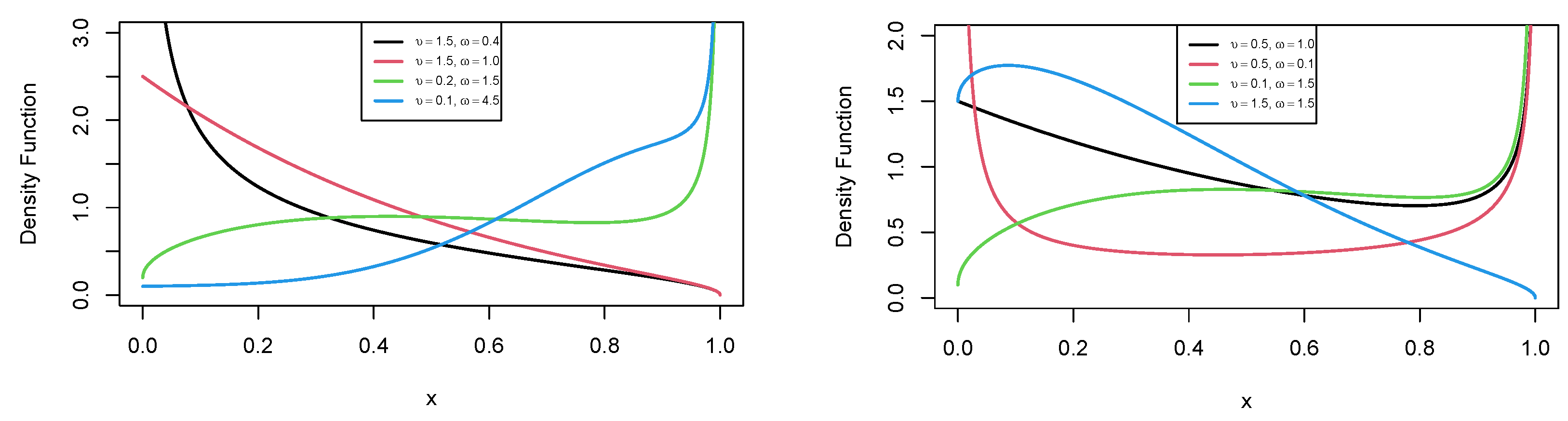
Indeed, an important characteristic of the MU distribution is that its pdf can be monotonically decreasing, increasing, unimodal, bathtub, and N-shaped, i.e., strictly increasing, and then followed by a bathtub shape. The plots of this pdf for different parameter values are given in Figure 2.

Figure 2. Plots for the pdf of the MU distribution.

The hrf limits of the MU distribution as $x\to 0$ and $x\to 1$ are determined below. We have

$$\underset{x\to 0}{lim}\phi \left(x;\upsilon ,\omega \right)=\left\{\begin{array}{c}\infty \omega <1,\hfill \\ \upsilon +\omega \omega =1,\mathrm{and}\underset{x\to 1}{lim}\phi \left(x;\upsilon ,\omega \right)=\infty .\hfill \\ \upsilon \omega >1\hfill \end{array}\right.$$

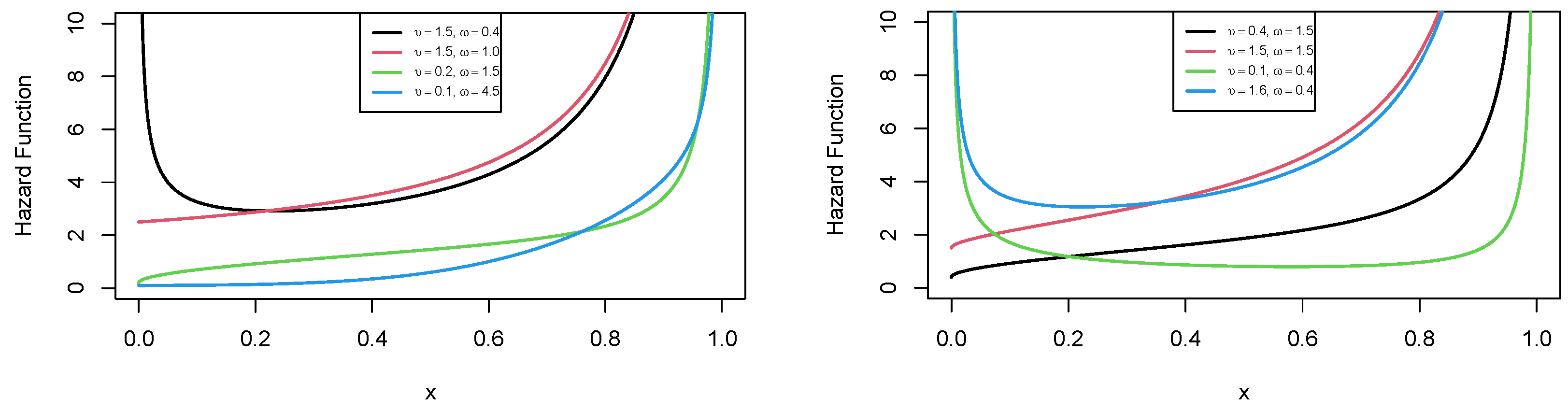
The following theorem shows mathematically that the hrf of the MU distribution can be increasing- or bathtub-shaped.

Theorem 1. 

The hrf of the MU distribution is increasing-shaped for $\omega \ge 1$ and is bathtub-shaped for $\omega <1$ for all values of υ.

Proof. 

From Equation (25), we have

$$\phi {}^{\prime }\left(x;\upsilon ,\omega \right)=\upsilon {\left(1-x\right)}^{-2}+\omega \left(\omega -1\right)x^{\omega -2}.$$

For $\omega \ge 1$, $\phi {}^{\prime }\left(x;\upsilon ,\omega \right)>0$, as a result, the hrf is increasing-shaped. On the other hand, the roots of $\phi {}^{\prime }\left(x;\upsilon ,\omega \right)$ exist and are unique for $\omega <1$; then, the hrf is bathtub-shaped since $\underset{x\to 0}{lim}\phi \left(x;\upsilon ,\omega \right)=\underset{x\to 1}{lim}\phi \left(x;\upsilon ,\omega \right)=\infty$. This ends the proof.    □

Additionally, it is noted that the hrf of the MU distribution cannot be decreasing-shaped.

The shape of the hrf, which can be monotonically increasing- or bathtub-shaped, depends only on the value of $\omega$. The plots of the hrf of the MU distribution for different parameter values are given in Figure 3, supporting the findings of Theorem 1.

Figure 3. Plots for the hrf of the MU distribution.

5. Properties of the MU Distribution

In the following subsections, we present some basic statistical features of the MU distribution. Hereafter, X denotes a random variable that has this distribution.

5.1. Moments

The following theorem proposes a manageable expansion of the $r^{th}$ raw moment of X depending on values of the standard beta function.

Theorem 2. 

For any integer $r\ge 0$, the $r^{th}$ raw moment of X is obtained by

$${\mu }_r^{{}^{\prime }}=E\left(X^r\right)=\sum _{i=0}^{\infty }\frac{{\left(-1\right)}^i}{i!}\left[\upsilon B\left(i\omega +r+1,\upsilon \right)+\omega B\left(\left(i+1\right)\omega +r,\upsilon +1\right)\right].$$

(26)

Proof. 

The classical exponential series expansion can be formulated as

$$e^{-x^{\omega }}=\sum _{i=0}^{\infty }\frac{{\left(-1\right)}^i}{i!}{x}^{i\omega },$$

for any $x\in \mathbb{R}$. Substituting in Equation (24), the following expansion holds:

$$f\left(x;\upsilon ,\omega \right)=\sum _{i=0}^{\infty }\frac{{\left(-1\right)}^i}{i!}\left(\upsilon +\omega \left(1-x\right)x^{\omega -1}\right){\left(1-x\right)}^{\upsilon -1}{x}^{i\omega }.$$

(27)

Using direct integration, the $r^{th}$ moment of X reduces to

$$\begin{array}{cc}\hfill {\mu }_r^{{}^{\prime }}& ={\int }_0^1{x}^{r}f\left(x;\upsilon ,\omega \right)dx\hfill \\ \hfill & =\sum _{i=0}^{\infty }\frac{{\left(-1\right)}^i}{i!}{\int }_0^1\left(\upsilon +\omega \left(1-x\right)x^{\omega -1}\right){\left(1-x\right)}^{\upsilon -1}{x}^{i\omega +r}dx\hfill \\ \hfill & =\sum _{i=0}^{\infty }\frac{{\left(-1\right)}^i}{i!}\left(\upsilon {\int }_0^1{x}^{i\omega +r}{\left(1-x\right)}^{\upsilon -1}dx+\omega {\int }_0^1{x}^{\left(i+1\right)\omega +r-1}{\left(1-x\right)}^{\upsilon }dx\right)\hfill \\ \hfill & =\sum _{i=0}^{\infty }\frac{{\left(-1\right)}^i}{i!}\left[\upsilon B\left(i\omega +r+1,\upsilon \right)+\omega B\left(\left(i+1\right)\omega +r,\upsilon +1\right)\right].\hfill \end{array}$$

This completes the proof of the theorem.    □

Remark 1. 

For the very special case where υ is a nonnegative integer, we can deal with the raw moments defined with finite sums and the incomplete gamma function. Indeed, we can write $f\left(x;\upsilon ,\omega \right)$ using the standard binomial formula for ${\left(1-x\right)}^{\upsilon -1}$ and ${\left(1-x\right)}^{\upsilon }$ as

$$\begin{array}{cc}\hfill f\left(x;\upsilon ,\omega \right)& =\upsilon \sum _{i=0}^{\upsilon -1}{(-1)}^i{x}^i{e}^{-x^{\omega }}+\omega \sum _{i=0}^{\upsilon }{(-1)}^i{x}^{i+\omega -1}{e}^{-x^{\omega }}.\hfill \end{array}$$

As a result of integrating over $(0,1)$ and changing the variables $y=x^{\omega }$, we have

$$\begin{array}{cc}\hfill {\mu }_r^{{}^{\prime }}& =\frac{\upsilon }{\omega }\sum _{i=0}^{\upsilon -1}{(-1)}^i\gamma \left(\frac{r+i+1}{\omega },1\right)+\sum _{i=0}^{\upsilon }{(-1)}^i\gamma \left(\frac{r+i}{\omega }+1,1\right),\hfill \end{array}$$

where $\gamma (a,x)={\int }_0^x{t}^{a-1}{e}^{-t}dt$ is the incomplete gamma function.

Based on Theorem 2, by adopting a computational viewpoint, we can approximate ${\mu }_r^{{}^{\prime }}$ as

$$\begin{array}{cc}\hfill {\mu }_r^{{}^{\prime }}& \approx \sum _{i=0}^I\frac{{\left(-1\right)}^i}{i!}\left[\upsilon B\left(i\omega +r+1,\upsilon \right)+\omega B\left(\left(i+1\right)\omega +r,\upsilon +1\right)\right],\hfill \end{array}$$

where I denotes a large but practical integer, say the arbitrary value of $I=40$. In addition, the mean X is obtained as $\mu ={\mu }_1^{{}^{\prime }}$, the variance of X follows from ${\mu }_2^{{}^{\prime }}$ and $\mu$ by using the Koenig–Huygens formula, and the central moments are derived from the following formula:

$$\begin{array}{c}\hfill {\mu }_r=E\left[{(X-\mu )}^r\right]=\sum _{j=0}^r\left(\genfrac{}{}{0pt}{}{r}{j}\right){(-1)}^j{\mu }^j{\mu }_{r-j}^{{}^{\prime }}.\end{array}$$

(28)

Using these central moments, the coefficients of kurtosis and asymmetry of X can be obtained according to the following relations, respectively:

$$\begin{array}{c}\hfill {\beta }_2=\frac{{\mu }_4}{{\mu }_2^2}=\frac{{\mu }_4^{{}^{\prime }}-4{\mu }_3^{{}^{\prime }}\mu +6{\mu }_2^{{}^{\prime }}{\mu }^2-3{\mu }^4}{{\left({\mu }_2^{{}^{\prime }}-{\mu }^2\right)}^2}\end{array}$$

(29)

and

$$\begin{array}{c}\hfill \sqrt{{\beta }_1}=\frac{{\mu }_3}{{\mu }_2^{3/2}}=\frac{{\mu }_3^{{}^{\prime }}-3{\mu }_2^{{}^{\prime }}\mu +2{\mu }^3}{{\left({\mu }_2^{{}^{\prime }}-{\mu }^2\right)}^{3/2}}.\end{array}$$

(30)

Table 1 presents some important moment measures of X for various parameter combinations, and it can be seen that the proposed distribution may be right-skewed or left-skewed, and platy-, meso- or lepto-kurtic, according to the values of $\upsilon$ and $\omega$.

Table 1. Some moment measures of X for various parameter combinations.

Actual Values		Mean	Variance	Kurtosis	Asymmetry
$\mathbf{\upsilon }$	$\mathbf{\omega }$
0.05	0.05	0.3684	0.2150	1.3509	0.5435
	0.20	0.4204	0.2003	1.2686	0.6065
	2.00	0.7196	0.0774	2.1643	−0.6270
	3.50	0.7971	0.0478	3.3934	−1.0417
0.20	0.05	0.3237	0.1819	1.6746	0.7206
	0.20	0.3731	0.1713	1.5166	−0.1995
	2.00	0.6494	0.0818	1.9664	−0.3867
	3.50	0.7166	0.0642	2.7795	−0.7920
2.00	0.05	0.1338	0.0467	4.8759	1.6895
	0.20	0.1656	0.0470	4.2450	1.4378
	2.00	0.3042	0.0459	2.6757	0.6525
	3.50	0.3221	0.0498	2.4263	0.5397
3.50	0.05	0.0907	0.0235	6.7032	2.0990
	0.20	0.1157	0.0243	2.9443	1.7159
	2.00	0.2109	0.0275	3.5139	0.9722
	3.50	0.2191	0.0297	3.3167	0.9246

Remark 2. 

The following elaborated formula can be used to provide an alternative result of Theorem 2: ${\mu }_r^{{}^{\prime }}=r{\int }_0^1{x}^{r-1}\left[1-F\left(x;\upsilon ,\omega \right)\right]dx$, which is valid in our setting for $r\ge 1$. It gives

$$\begin{array}{cc}\hfill {\mu }_r^{{}^{\prime }}& =r{\int }_0^1{x}^{r-1}{\left(1-x\right)}^{\upsilon }{e}^{-x^{\omega }}dx=r\sum _{i=0}^{\infty }\frac{{\left(-1\right)}^i}{i!}{\int }_0^1{x}^{i\omega +r-1}{\left(1-x\right)}^{\upsilon }dx\hfill \\ \hfill & =r\sum _{i=0}^{\infty }\frac{{\left(-1\right)}^i}{i!}B\left(i\omega +r,\upsilon +1\right).\hfill \end{array}$$

This formula is simpler than those in Theorem 2, but the moment techniques are not easily transposable to other moments measures, such as those presented in the following.

We complete this moment study by indicating a possible expansion for the moment generating function (mgf) of X. First, a well-known expansion gives

$$M\left(t\right)=E\left(e^{tX}\right)=\sum _{r=0}^{\infty }\frac{t^r}{r!}{\mu }_r^{{}^{\prime }},$$

(31)

where $t\in \mathbb{R}$.

Making use of Theorem 2, the mgf of X has the form

$$M\left(t\right)=\sum _{r=0}^{\infty }\sum _{i=0}^{\infty }\frac{{\left(-1\right)}^i{t}^r}{i!r!}\left[\upsilon B(i\omega +r+1,\upsilon )+\omega B\left(\right(i+1)\omega +r,\upsilon +1)\right],$$

(32)

where $t\in \mathbb{R}$.

5.2. Quantile Function

The solution of the following nonlinear equation yields the expression for the $q^{th}$ quantile of the MU distribution, say $x_q$:

$$\upsilon log\left(1-x_q\right)-x_q^{\omega }-log\left(1-q\right)=0.$$

(33)

This solution can only be determined numerically. By setting $q=0.5$ in Equation (33), one can obtain the median (M) of the MU distribution. Furthermore, the lower and higher quartiles can be obtained by setting $q=0.25$ and $q=0.75$, respectively.

5.3. Mean Deviation

The theorem below investigates an expansion of the mean deviation (MD) of X about the mean and the one about the median in terms of the values of the incomplete beta function.

Theorem 3. 

The MD of X about the mean and the median can be expanded as, respectively,

$$\begin{array}{cc}\hfill MD\left(\mu \right)& =E\left(\right|X-\mu \left|\right)=2\mu F\left(\mu ;\upsilon ,\omega \right)\hfill \\ \hfill & -2\sum _{i=0}^{\infty }\frac{{\left(-1\right)}^i}{i!}\left(\upsilon B_{\mu }\left(i\omega +2,\upsilon \right)+\omega B_{\mu }\left(\left(i+1\right)\omega +1,\upsilon +1\right)\right)\hfill \end{array}$$

(34)

and

$$\begin{array}{cc}\hfill MD\left(M\right)& =E\left(\right|X-M\left|\right)=2MF\left(M;\upsilon ,\omega \right)+\mu -M\hfill \\ \hfill & -2\sum _{i=0}^{\infty }\frac{{\left(-1\right)}^i}{i!}\left(\upsilon B_{\mu }\left(i\omega +2,\upsilon \right)+\omega B_{\mu }\left(\left(i+1\right)\omega +1,\upsilon +1\right)\right),\hfill \end{array}$$

(35)

where $B_x\left(a,b\right)={\int }_0^x{t}^{a-1}{\left(1-t\right)}^{b-1}dt$ is the incomplete beta function.

Proof. 

By the definition of the MD about the mean, we have

$$\begin{array}{cc}\hfill MD\left(\mu \right)& ={\int }_0^1\left|x-\mu \right|f\left(x;\upsilon ,\omega \right)dx\hfill \\ \hfill & ={\int }_0^{\mu }\left(\mu -x\right)f\left(x;\upsilon ,\omega \right)dx+{\int }_{\mu }^1\left(x-\mu \right)f\left(x;\upsilon ,\omega \right)dx.\hfill \end{array}$$

After simplification, we have

$$MD\left(\mu \right)=2\mu F\left(\mu ;\upsilon ,\omega \right)-2{\int }_0^{\mu }xf\left(x;\upsilon ,\omega \right)dx.$$

(36)

The result in Equation (34) follows upon substitution of Equation (27) into Equation (36). On the other hand, by the definition of the MD about the median, we also have

$$\begin{array}{cc}\hfill MD\left(M\right)& ={\int }_0^1\left|x-M\right|f\left(x;\upsilon ,\omega \right)dx\hfill \\ \hfill & ={\int }_0^M\left(M-x\right)f\left(x;\upsilon ,\omega \right)dx+{\int }_M^1\left(x-M\right)f\left(x;\upsilon ,\omega \right)dx\hfill \\ \hfill & =2MF\left(M;\upsilon ,\omega \right)+\mu -M-2{\int }_0^{M}xf\left(x;\upsilon ,\omega \right)dx.\hfill \end{array}$$

(37)

Substituting Equation (27) into Equation (37), we obtain the result in Equation (35).    □

5.4. Order Statistics

Order statistics of a given distribution naturally appear in various random systems and estimation methods. Here, some of their basic distributional properties in the context of the MU distribution are presented. Let $X_{\left(1\right)},X_{\left(2\right)},\dots ,X_{\left(n\right)}$ be the order statistics obtained from a random sample from the MU distribution with parameters $\upsilon$ and $\omega$. Then, the pdf of the $k^{th}$ order statistic, say $X_{\left(k\right)}$, is defined as

$$f_{\left(k\right)}\left(x;\upsilon ,\omega \right)=\frac{1}{B\left(k,n-k+1\right)}{\left[F\left(x;\upsilon ,\omega \right)\right]}^{k-1}{\left[\overline{F}\left(x;\upsilon ,\omega \right)\right]}^{n-k}f\left(x;\upsilon ,\omega \right).$$

(38)

It can be simplified as

$$f_{\left(k\right)}\left(x;\upsilon ,\omega \right)=\frac{1}{B\left(k,n-k+1\right)}\sum _{j=0}^{k-1}\left(\genfrac{}{}{0pt}{}{k-1}{j}\right){\left(-1\right)}^j{\left[\overline{F}\left(x;\upsilon ,\omega \right)\right]}^{n+j-k}f\left(x;\upsilon ,\omega \right).$$

(39)

On the ther hand, the cdf of $X_{\left(k\right)}$ can be expressed as

$$F_{\left(k\right)}\left(x;\upsilon ,\omega \right)=\sum _{j=k}^n\left(\genfrac{}{}{0pt}{}{n}{j}\right){\left[F\left(x;\alpha ,\theta \right)\right]}^j{\left[\overline{F}\left(x;\upsilon ,\omega \right)\right]}^{n-j},$$

(40)

which can be reduced to

$$F_{\left(k\right)}\left(x;\upsilon ,\omega \right)=\sum _{j=k}^n\sum _{l=0}^j\left(\genfrac{}{}{0pt}{}{n}{j}\right)\left(\genfrac{}{}{0pt}{}{j}{l}\right){\left(-1\right)}^l{\left[\overline{F}\left(x;\upsilon ,\omega \right)\right]}^{n+l-j}.$$

(41)

Using Equations (23) and (24) and the series expansion, then the pdf and cdf of $X_{\left(k\right)}$ have the following infinite polynomial series expansions, respectively:

$$f_{\left(k\right)}\left(x;\upsilon ,\omega \right)=\frac{\upsilon +\omega \left(1-x\right)x^{\omega -1}}{B\left(k,n-k+1\right)}\sum _{j=0}^{k-1}\sum _{l=0}^{\infty }\sum _{m=0}^{\infty }\left(\genfrac{}{}{0pt}{}{k-1}{j}\right)\left(\genfrac{}{}{0pt}{}{a\upsilon -1}{l}\right)\frac{{(-1)}^{j+l+m}}{m!}{x}^{\omega m+l}{a}^m$$

(42)

and

$$F_{\left(k\right)}\left(x;\alpha ,\theta \right)=\sum _{j=k}^n\sum _{l=0}^j\sum _{i=0}^{\infty }\sum _{m=0}^{\infty }\left(\genfrac{}{}{0pt}{}{n}{j}\right)\left(\genfrac{}{}{0pt}{}{j}{l}\right)\left(\genfrac{}{}{0pt}{}{b\upsilon }{i}\right)\frac{{(-1)}^{l+i+m}}{m!}{b}^m{x}^{m\omega +i},$$

(43)

where $a=n+j-k+1$ and $b=n+l-j$.

These simple polynomial expansions open the door for more manipulation of the characteristics of $X_{\left(k\right)}$, especially its moment properties.

The pdf and cdf of the distributions of the minimum and the maximum order statistics of the MU distribution are obtained from Equations (42) and (43) with $k=1$ and $k=n$, respectively.

6. Estimation of the Parameters of the MU Model

We are now in position to estimate the parameters of the MU model using different techniques.

6.1. Maximum Likelihood Estimates

In the following, the estimation of unknown parameters of the MU model by the maximum likelihood (ML) is derived. Suppose that $X_1,X_2,\dots ,X_n$ forms a random sample from the MU distribution, and $x_1,x_2,\dots ,x_n$ are their respective observations. Then, the log likelihood function is given by

$$L\left(\upsilon ,\omega \right)=\left(\upsilon -1\right)\sum _{i=1}^{n}log\left(1-x_i\right)+\sum _{i=1}^{n}log\left[\upsilon +\omega \left(1-x_i\right)x_i^{\omega -1}\right]-\sum _{i=1}^n{x}_i^{\omega }.$$

(44)

The ML estimates (MLEs) of $\upsilon$ and $\omega$ can be obtained by maximizing $L\left(\upsilon ,\omega \right)$ with respect to $\upsilon$ and $\omega$, respectively. In our case, this is equivalent to solve simultaneously the following nonlinear equations: $\partial L\left(\upsilon ,\omega \right)/\partial \upsilon =0$ and $\partial L\left(\upsilon ,\omega \right)/\partial \omega =0$. Hereafter, for the sake of readability, the involved partial derivatives are expressed in Appendix A.

6.2. Least-Squares and Weighted Least-Squares Estimates

Swain et al. [12] introduced the least-squares (LS) and the weighted LS (WLS) methods. The LS estimates (LSEs) of the parameters of the MU model can be obtained by minimizing the following error function:

$$LS\left(\upsilon ,\omega \right)=\sum _{i=1}^n{\left(F\left(x_{\left(i\right)};\upsilon ,\omega \right)-\frac{i}{n+1}\right)}^2,$$

(45)

with respect to $\upsilon$ and $\omega$, where $x_{\left(i\right)}$ is the $i^{\mathrm{th}}$ smallest observation among $x_1,x_2,\dots ,x_n$. This is equivalent to solve simultaneously the following nonlinear equations: $\partial LS\left(\upsilon ,\omega \right)/\partial \upsilon =0$ and $\partial LS\left(\upsilon ,\omega \right)/\partial \omega =0$.

On the other hand, Gupta and Kundu [13] introduced the WLS estimates (WLSEs), obtained by minimizing the following error function:

$$WLS\left(\upsilon ,\omega \right)=\sum _{i=1}^n\frac{{\left(n+1\right)}^2\left(n+2\right)}{i\left(n-i+1\right)}{\left(F\left(x_{\left(i\right)};\upsilon ,\omega \right)-\frac{i}{n+1}\right)}^2,$$

(46)

with respect to the unknown parameters. As a result, we can determine them by solving the following nonlinear equations: $\partial WLS\left(\upsilon ,\omega \right)/\partial \upsilon =0$ and $\partial WLS\left(\upsilon ,\omega \right)/\partial \omega =0$.

6.3. Maximum Product of Spacing Estimates

Cheng and Amin [14] proposed the maximum product of spacing (MPS) method based on the geometric mean function of the differences defined by

$$GM\left(\upsilon ,\omega \right)=\sqrt[n+1]{\prod _{i=1}^{n+1}\left(F\left(x_{\left(i\right)};\upsilon ,\omega \right)-F\left(x_{\left(i-1\right)};\upsilon ,\omega \right)\right)},$$

(47)

where $F\left(x_{\left(0\right)};\upsilon ,\omega \right)=0$ and $F\left(x_{\left(n+1\right)};\upsilon ,\omega \right)=1$. Its logarithmic transformation is defined by

$$logGM\left(\upsilon ,\omega \right)=\frac{1}{n+1}\sum _{i=1}^{n+1}log\left(F\left(x_{\left(i\right)};\upsilon ,\omega \right)-F\left(x_{\left(i-1\right)};\upsilon ,\omega \right)\right).$$

(48)

Maximizing this function with respect to $\upsilon$ and $\omega$ yields the MPS estimates (MPSEs). We can determine them by solving the following nonlinear equations: $\partial logGM\left(\upsilon ,\omega \right)/\partial \upsilon =0$ and $\partial logGM\left(\upsilon ,\omega \right)/\partial \omega =0$.

6.4. Cramér–von Mises Estimates

As a type of minimum distance estimation method, Choi and Bulgren [15] introduced the Cramér–von Mises (CM) method. This method depends on the CM statistic, which, according to [16], can be written as

$$C\left(\upsilon ,\omega \right)=\frac{1}{12n}+\sum _{i=1}^n{\left(F\left(x_{\left(i\right)};\upsilon ,\omega \right)-\frac{2i-1}{2n}\right)}^2.$$

(49)

Then, the CM estimates (CMEs) can be obtained by minimizing the CM statistic with respect to $\upsilon$ and $\omega$. We can find them by solving the following nonlinear equations: $\partial C\left(\upsilon ,\omega \right)/\partial \upsilon =0$ and $\partial C\left(\upsilon ,\omega \right)/\partial \omega =0$.

6.5. Anderson–Darling and Right-Tail Anderson–Darling Estimates

The Anderson–Darling (AD) method was introduced by Anderson and Darling [17,18] and it depends on the AD statistic, which, according to [16], can be calculated as

$$A\left(\upsilon ,\omega \right)=-n-\frac{1}{n}\sum _{i=1}^n\left(2i-1\right)\left[logF\left(x_{\left(i\right)};\upsilon ,\omega \right)+log\left(1-F\left(x_{\left(i\right)};\upsilon ,\omega \right)\right)\right].$$

(50)

Therefore, AD estimates (ADEs) can be obtained by minimizing the AD statistic with respect to $\upsilon$ and $\omega$. We can evaluate them by solving the following nonlinear equations: $\partial A\left(\upsilon ,\omega \right)/\partial \upsilon =0$ and $\partial A\left(\upsilon ,\omega \right)/\partial \omega =0$.

On the other hand, Luceno [19] applied some modifications on the AD statistic to define the right-tail Anderson–Darling (RAD) statistic, which is specified by

$$RA\left(\upsilon ,\omega \right)=\frac{n}{2}-2\sum _{i=1}^{n}F\left(x_{\left(i\right)};\upsilon ,\omega \right)-\frac{1}{n}\sum _{i=1}^n\left(2i-1\right)log\left(1-F\left(x_{\left(i\right)};\upsilon ,\omega \right)\right).$$

(51)

The RAD estimates (RADEs) are obtained by minimizing the RAD statistic with respect to $\upsilon$ and $\omega$. We can determine them by solving the following nonlinear equations: $\partial RA\left(\upsilon ,\omega \right)/\partial \upsilon =0$ and $\partial RA\left(\upsilon ,\omega \right)/\partial \omega =0$.

Note that all the above nonlinear systems do not have explicit solutions, so we use the nlminb and optim functions in R software to solve them.

7. Simulation Analysis

Now, a simulation study is performed to verify the performance and efficiency of the different estimates of the parameters of the MU model. Different sample sizes, n, and several values of the unknown parameters $\upsilon$ and $\omega$ are considered, and each scenario is replicated 5000 times. The procedure for evaluating the suggested estimates is as follows:

(1)

Initialize n, $\upsilon$, and $\omega$.

(2)

Generate a sample of observations from the MU distribution of size n.

(3)

The outcomes in step 2 are used to compute the $\widehat{\Theta }=\left(\widehat{\upsilon },\widehat{\omega }\right)$ considering the MLEs, LSEs, WLSEs, MPSEs, CMEs, ADEs, and RADEs.

(4)

The above steps are repeated $5000$ times.

(5)

Using $\widehat{\Theta }$ and $\Theta$, compute the biases and the mean squared errors (MSEs).

The bias and MSEs of the MLEs, LSEs, WLSEs, CMEs, and MPSEs are reported in Table 2, Table 3 and Table 4. The partial and overall ranks of these estimates are calculated in Table 5. From these tables, it is noted that:

Table 2. Bias and MSEs of different estimates for $\upsilon =0.4$ and $\omega =1$.

n	Est.	Est. Par.	MLEs	LSEs	WLSEs	MPSEs	CMEs	ADEs	RADEs
20	Bias	$\widehat{\upsilon }$	0.1086	0.0478	0.0520	0.2254	0.1176	0.0717	0.0831
		$\widehat{\omega }$	0.5467	0.2139	0.7280	0.6676	0.5030	0.4216	0.6893
	MSEs	$\widehat{\upsilon }$	0.0662	0.0796	0.0665	0.1385	0.1085	0.0590	0.0642
		$\widehat{\omega }$	7.5127	2.1804	8.7361	11.4240	5.4094	8.4160	12.0124
50	Bias	$\widehat{\upsilon }$	0.0476	0.0186	0.0255	0.0883	0.0430	0.0300	0.0327
		$\widehat{\omega }$	0.1424	0.0517	0.0844	0.1372	0.1253	0.0541	0.1439
	MSEs	$\widehat{\upsilon }$	0.0142	0.0254	0.0215	0.0279	0.0300	0.0158	0.0146
		$\widehat{\omega }$	3.5215	0.2140	0.3556	2.8197	0.4101	0.1485	2.1318
100	Bias	$\widehat{\upsilon }$	0.0288	0.0069	0.0122	0.0467	0.0224	0.0158	0.0179
		$\widehat{\omega }$	0.0294	0.0197	0.0218	0.0139	0.0420	0.0192	0.0391
	MSEs	$\widehat{\upsilon }$	0.0049	0.0105	0.0082	0.0085	0.0120	0.0055	0.0053
		$\widehat{\omega }$	0.0580	0.0453	0.0262	0.0957	0.0413	0.0187	0.0690
200	Bias	$\widehat{\upsilon }$	0.0135	0.0031	0.0073	0.0254	0.0093	0.0085	0.0084
		$\widehat{\omega }$	0.0065	0.0086	0.0104	−0.0019	0.0198	0.0080	0.0128
	MSEs	$\widehat{\upsilon }$	0.0014	0.0048	0.0039	0.0030	0.0052	0.0017	0.0015
		$\widehat{\omega }$	0.0082	0.0137	0.0122	0.0094	0.0144	0.0049	0.0081

Table 3. Bias and MSEs of different estimates for $\upsilon =0.5$ and $\omega =0.8$.

n	Est.	Est. Par.	MLEs	LSEs	WLSEs	MPSEs	CMEs	ADEs	RADEs
20	Bias	$\widehat{\upsilon }$	0.1314	0.0608	0.0624	0.2566	0.1476	0.0781	0.0581
		$\widehat{\omega }$	0.4218	0.1765	0.2175	0.4157	0.3217	0.2250	0.2795
	MSEs	$\widehat{\upsilon }$	0.1098	0.1215	0.1104	0.1942	0.1679	0.0904	0.0537
		$\widehat{\omega }$	5.1726	1.2522	1.5926	6.8543	2.4182	5.3634	3.7420
50	Bias	$\widehat{\upsilon }$	0.0490	0.0164	0.0245	0.1043	0.0512	0.0291	0.0343
		$\widehat{\omega }$	0.0864	0.0369	0.0431	0.0410	0.0905	0.0459	0.0799
	MSEs	$\widehat{\upsilon }$	0.0217	0.0349	0.0301	0.0391	0.0424	0.0255	0.0251
		$\widehat{\omega }$	0.5554	0.0837	0.0759	0.6855	0.7412	0.2166	0.2312
100	Bias	$\widehat{\upsilon }$	0.0250	0.0094	0.0154	0.0537	0.0240	0.0186	0.0160
		$\widehat{\omega }$	0.0241	0.0125	0.0182	−0.0001	0.0328	0.0170	0.0281
	MSEs	$\widehat{\upsilon }$	0.0076	0.0156	0.0123	0.0127	0.0166	0.0104	0.0092
		$\widehat{\omega }$	0.0126	0.0179	0.0171	0.2245	0.0237	0.0165	0.0218
200	Bias	$\widehat{\upsilon }$	0.0165	0.0045	0.0068	0.0278	0.0124	0.0074	0.0095
		$\widehat{\omega }$	0.0106	0.0059	0.0063	−0.0055	0.0136	0.0065	0.0126
	MSEs	$\widehat{\upsilon }$	0.0033	0.0072	0.0057	0.0050	0.0076	0.0039	0.0039
		$\widehat{\omega }$	0.0045	0.0076	0.0067	0.0056	0.0087	0.0049	0.0081

Table 4. Bias and MSEs of different estimates for $\upsilon =2$ and $\omega =0.5$.

n	Est.	Est. Par.	MLEs	LSEs	WLSEs	MPSEs	CMEs	ADEs	RADEs
20	Bias	$\widehat{\upsilon }$	0.3416	0.1249	0.1318	0.6876	0.4190	0.1953	0.2465
		$\widehat{\omega }$	0.2355	0.0906	0.0984	0.0779	0.1987	0.1647	0.2290
	MSEs	$\widehat{\upsilon }$	0.9177	1.0823	0.9232	1.5692	1.4522	0.7830	0.9127
		$\widehat{\omega }$	0.5661	0.1632	0.1905	0.2282	0.2904	2.7567	0.4853
50	Bias	$\widehat{\upsilon }$	0.1108	0.0585	0.0696	0.2387	0.1738	0.0624	0.0952
		$\widehat{\omega }$	0.0679	0.0278	0.0353	0.0141	0.0584	0.0313	0.0673
	MSEs	$\widehat{\upsilon }$	0.2159	0.3536	0.2992	0.2895	0.4113	0.2280	0.2922
		$\widehat{\omega }$	0.1599	0.0481	0.1490	0.0330	0.0680	0.0323	0.1161
100	Bias	$\widehat{\upsilon }$	0.0437	0.0374	0.0363	0.1036	0.0711	0.0305	0.0458
		$\widehat{\omega }$	0.0253	0.0089	0.0088	0.0091	0.0208	0.0137	0.0220
	MSEs	$\widehat{\upsilon }$	0.0758	0.1456	0.1313	0.0942	0.1705	0.0813	0.1202
		$\widehat{\omega }$	0.0087	0.0096	0.0072	0.0030	0.0127	0.0046	0.0168
200	Bias	$\widehat{\upsilon }$	0.0162	0.0109	0.0251	0.0395	0.0408	0.0110	0.0212
		$\widehat{\omega }$	0.0128	0.0027	0.0059	0.0071	0.0088	0.0065	0.0076
	MSEs	$\widehat{\upsilon }$	0.0240	0.0729	0.0637	0.0265	0.0768	0.0277	0.0578
		$\widehat{\omega }$	0.0014	0.0033	0.0028	0.0009	0.0037	0.0013	0.0058

Table 5. Partial and overall ranks of all estimation methods for various combinations of $\upsilon$ and $\omega$.

Initial Values	n	MLEs		LSEs		WLSEs		MPSEs		CMEs		ADEs		RADEs
		$\widehat{\mathbf{\upsilon }}$	$\widehat{\mathbf{\omega }}$	$\widehat{\mathbf{\upsilon }}$	$\widehat{\mathbf{\omega }}$	$\widehat{\mathbf{\upsilon }}$	$\widehat{\mathbf{\omega }}$	$\widehat{\mathbf{\upsilon }}$	$\widehat{\mathbf{\omega }}$	$\widehat{\mathbf{\upsilon }}$	$\widehat{\mathbf{\omega }}$	$\widehat{\mathbf{\upsilon }}$	$\widehat{\mathbf{\omega }}$	$\widehat{\mathbf{\upsilon }}$	$\widehat{\mathbf{\omega }}$
$\upsilon =0.4$ and $\omega =1$	50	3	5	5	1	4	2	7	7	6	3	2	6	1	4
	100	1	5	5	2	4	1	6	6	7	7	3	3	2	4
	150	1	1	6	4	4	3	5	7	7	6	3	2	2	5
	200	1	1	6	5	5	4	4	3	7	7	2	2	2	6
$\upsilon =0.5$ and $\omega =0.8$	50	3	6	5	1	4	2	7	3	6	4	1	7	2	5
	80	1	7	6	3	5	6	3	2	7	4	2	1	4	5
	120	1	4	6	5	5	3	3	1	7	6	2	2	4	7
	200	1	3	6	5	5	4	2	1	7	6	3	2	4	7
$\upsilon =2$ and $\omega =0.5$	50	3	3	5	1	4	5	7	6	6	2	1	4	2	7
	80	1	7	5	2	4	3	6	6	7	4	3	1	2	5
	120	1	5	6	4	4	2	5	7	7	3	3	1	2	6
	200	1	3	6	6	5	5	4	4	7	7	3	1	2	2
Sum		18	50	67	39	53	40	59	53	81	59	28	32	29	63
Overall Rank		1	4	6	2	4	3	5	5	7	6	2	1	3	7

• All estimates show the property of consistency, i.e., the MSEs decrease as the sample size increases for all the parameter combinations.
• According to the MSEs, the ordering of performance of the estimates (from best to worst) for $\upsilon$ is MLEs, ADEs, RADEs, WLSEs, MPSEs, LSEs, and CMEs.
• In addition, the ordering of performance of the estimates (from best to worst) for $\omega$ is ADEs, LSEs, WLSEs, MLEs, MPSEs, CMEs, and RADEs.

8. Real Data Applications

In this part, we analyze two real data sets to demonstrate the performance of the MU model in practice by fitting two real-life data sets. The proposed MU model is compared to models based on the following distributions: the K distribution, which is defined by the pdf in Equation (6) and other four known competitors such as

• Size-biased Kumaraswamy (SK) distribution [20] with pdf indicated as

  $$g\left(x;\upsilon ,\omega \right)=\frac{\upsilon x^{\upsilon }{\left(1-x^{\upsilon }\right)}^{\omega -1}}{B\left(\upsilon +1/\upsilon ,\omega \right)},\upsilon ,\omega >0,x\in \left(0,1\right).$$
• Exponentiated Kumaraswamy (EK) distribution [21] with pdf given as

  $$g\left(x;\upsilon ,\omega ,\theta \right)=\upsilon \omega x^{\upsilon -1}{\left(1-x^{\upsilon }\right)}^{\omega -1}{\left(1-{\left(1-x^{\upsilon }\right)}^{\omega }\right)}^{\theta -1},\upsilon ,\omega ,\theta >0,x\in \left(0,1\right).$$
• Transmuted Kumaraswamy (TK) distribution [22] with pdf specified by

  $$g\left(x;\upsilon ,\omega ,\theta \right)=\upsilon \omega x^{\upsilon -1}{\left(1-x^{\upsilon }\right)}^{\omega -1}\left(1-\theta +2\theta {\left(1-x^{\upsilon }\right)}^{\omega }\right),\upsilon ,\omega ,\theta >0,x\in \left(0,1\right).$$
• McDonald (M) distribution [23] with pdf given as

  $$g\left(x;\upsilon ,\omega ,\theta \right)=\frac{\upsilon x^{\upsilon \omega -1}{\left(1-x^{\upsilon }\right)}^{\theta -1}}{B\left(\omega ,\theta \right)},\upsilon ,\omega ,\theta >0,x\in \left(0,1\right).$$

The first data set is reported by Murthy et al. [24]. It represents censored data (failure times) for thirty items tested, with testing stopping after the 20^th failure. The second data set represents observations on the stress resistance shear (MPa) of a joint joined in a particular way. It is taken from Stoop and Ouden [25]. To determine the interval parameter ($\theta$, sometimes called the product maximum life), Wang [26] used the following formula:

$$\theta =x_n+\frac{x_n-x_{n-k}}{nk},$$

where n is the sample size, $x_n$ is the value of $n^{th}$ time of the sample, and k is the number of $x_n$ in the sample. By applying the above formula to two data sets, the summary of their statistical measures is listed in Table 6.

Table 6. Summary measures of the two data sets.

Data	Min	Q1	Median	Mean	Q3	SD	Skewness	Kurtosis	Max
First	0.1813	0.5419	0.6150	0.6480	0.8457	0.2413	−0.3187	−1.0937	0.9990
Second	0.0390	0.2320	0.3254	0.4161	0.6241	0.2846	0.5328	−1.0472	0.9770

Table 6. Summary measures of the two data sets.

Data	Min	Q1	Median	Mean	Q3	SD	Skewness	Kurtosis	Max
First	0.1813	0.5419	0.6150	0.6480	0.8457	0.2413	−0.3187	−1.0937	0.9990
Second	0.0390	0.2320	0.3254	0.4161	0.6241	0.2846	0.5328	−1.0472	0.9770

The MLEs of the parameters for the compared models are computed. In addition, the values of various discrimination measures are evaluated to provide model efficiency. These are the Akaike information criterion (AIC), defined as AIC $=2k-2log\left(\widehat{L}\right)$); Bayesian information criterion (BIC), defined as BIC $=klog\left(n\right)-2log\left(\widehat{L}\right)$); consistent-AIC (CAIC), defined as CAIC $=k(log\left(n\right)+1)-2log\left(\widehat{L}\right)$); and Hannan–Quinn information criterion (HQIC), defined as HQIC $=2klog(log\left(n\right))-2log\left(\widehat{L}\right)$), where k is the number of estimated parameters, n is the sample size, and $\widehat{L}$ is the maximum value of the corresponding likelihood function. Furthermore, the goodness of fit for the compared models is checked by various test statistics, such as the Cramér–von Mises $W_n^2$, Anderson–Darling $A_n^2$, Watson $U_n^2$, Liao–Shimokawa $L_n$, and sum of squares (SS). We also calculate the Kolmogorov–Smirnov (KS) statistics and their corresponding p-values. To check the fitting performance of the models (p-value > 0.05), these test statistics demonstrate the differences between the proposed cdf and the empirical cdf for each data set. For more details about the goodness-of-fit test statistics, the reader can see Shama et al. [27].

From Table 7 and Table 8, we note that the MU model gives the lowest values for all the discrimination measures. These results indicate that the MU model could be chosen as the best model against all the competitors. Table 9 and Table 10 show that all models fit two data sets (p-value > 0.05) and the proposed model displays the lowest test statistics with the highest p-values. As a result, the MU model offers excellent competition against other models and fits the two data sets quite well.

Table 7. The MLEs of the parameters for the compared models and the values of discrimination measures for the first data set.

Models	Estimates			Discrimination Measures
	$\widehat{\mathit{\upsilon }}$	$\widehat{\mathit{\omega }}$	$\widehat{\mathit{\theta }}$	AIC	BIC	CAIC	HQIC
MU	0.3928	3.3929	—	−3.3306	−1.3392	0.6608	−2.9419
K	1.7516	0.8672	—	−3.1823	−1.1908	0.8092	−2.7935
SK	0.7292	0.8800	—	−3.1423	−1.1509	0.8491	−2.7536
EK	12.7131	0.5891	0.1407	−1.9438	1.0434	4.0434	−1.3607
TK	1.9665	0.6472	0.6516	−2.1678	0.8194	3.8194	−1.5847
M	79.0770	0.0233	0.4316	−2.5092	0.4780	3.4780	−1.9261

Table 8. The MLEs of the parameters for the compared models and the values of discrimination measures for the second data set.

Models	Estimates			Discrimination Measures
	$\widehat{\mathit{\upsilon }}$	$\widehat{\mathit{\omega }}$	$\widehat{\mathit{\theta }}$	AIC	BIC	CAIC	HQIC
MU	0.7645	1.2811	—	2.5925	3.3883	5.3883	2.0909
K	0.9608	1.1957	—	3.5469	4.3427	6.3427	3.0453
SK	0.0416	1.2148	—	3.4947	4.2904	6.2904	2.9930
EK	0.0030	1.2194	917.5928	5.1641	6.3578	9.3578	4.4117
TK	1.0827	0.6001	0.9547	4.9668	6.1605	9.1605	4.2144
M	0.0646	16.1024	1.21521	5.4948	6.6885	9.6885	4.7424

Table 9. The values of goodness-of-fit test statistics for the first data set.

Models	${\mathit{W}}_{\mathit{n}}^2$	${\mathit{A}}_{\mathit{n}}^2$	${\mathit{U}}_{\mathit{n}}^2$	${\mathit{L}}_{\mathit{n}}$	SS	KS	KS p-Value
MU	0.0511	0.3305	4.5607	0.7147	0.0433	0.1163	0.9495
K	0.0645	0.3975	4.6060	0.8867	0.0587	0.1622	0.6687
SK	0.0632	0.3947	4.6040	0.8909	0.0575	0.1619	0.6708
EK	0.0648	0.3632	4.6065	0.7912	0.0583	0.1560	0.7154
TK	0.0465	0.2914	4.5765	0.7962	0.0417	0.1456	0.7901
M	0.0549	0.3010	4.5924	0.7313	0.0490	0.1529	0.7380

Table 10. The values of goodness-of-fit test statistics for the second data set.

Models	${\mathit{W}}_{\mathit{n}}^2$	${\mathit{A}}_{\mathit{n}}^2$	${\mathit{U}}_{\mathit{n}}^2$	${\mathit{L}}_{\mathit{n}}$	SS	KS	KS p-Value
MU	0.0419	0.2476	2.3367	0.7811	0.0325	0.1800	0.8684
K	0.0591	0.3640	2.3658	0.9259	0.0493	0.2076	0.7300
SK	0.0563	0.3552	2.3616	0.9216	0.0468	0.2050	0.7445
EK	0.0435	0.3095	2.3393	0.9205	0.0351	0.1867	0.8378
TK	0.0447	0.2855	2.3413	0.8472	0.0360	0.1885	0.8292
M	0.0563	0.3550	2.3615	0.9216	0.0468	0.2049	0.7449

Furthermore, seven estimation methods are used to estimate the parameters of the MU model from real data. Table 11 and Table 12 display the estimates, the values of $SS$ and $KS$ with their p-values, and the rank of estimation methods for the two data sets. We can draw the conclusion that, for the first data set, the ML estimation method is advised for estimating the unknown parameters of the proposed model, whereas the LS estimation method is advised for estimating the unknown parameters of the MU model.

Table 11. The estimates of the parameters of the MU model, SS, K-S, and p-value for the first data set.

Est. Meth.	Est. Par.		SS	KS	KS p-Value	Rank
	$\widehat{\mathbf{\upsilon }}$	$\widehat{\mathbf{\omega }}$
MLE	0.3928	3.3929	0.0433	0.1163	0.9495	1
LSE	0.3922	3.5206	0.0426	0.1189	0.9400	3
WLSE	0.3762	3.4002	0.0432	0.1214	0.9296	4
MPSE	0.5208	4.2605	0.0705	0.1470	0.7806	7
CME	0.4124	3.8164	0.0423	0.1217	0.9285	5
ADE	0.3994	3.6990	0.0425	0.1236	0.9201	6
RADE	0.4366	4.0096	0.0433	0.1165	0.9490	2

Table 12. The estimates of the parameters of the MU model, SS, K-S, and p-value for the second data set.

Est. Meth.	Est. Par.		SS	KS	KS p-Value	Rank
	$\widehat{\mathbf{\upsilon }}$	$\widehat{\mathbf{\omega }}$
MLE	0.7645	1.2811	0.0325	0.1800	0.8684	7
LSE	0.7489	1.0733	0.0287	0.1499	0.9658	1
WLSE	0.6912	1.0326	0.0308	0.1558	0.9522	4
MPSE	1.4283	2.0801	0.0478	0.1660	0.9224	6
CME	0.9472	1.3849	0.0264	0.1513	0.9627	3
ADE	0.7991	1.2215	0.0276	0.1627	0.9329	5
RADE	0.7306	1.0507	0.0294	0.1501	0.9654	2

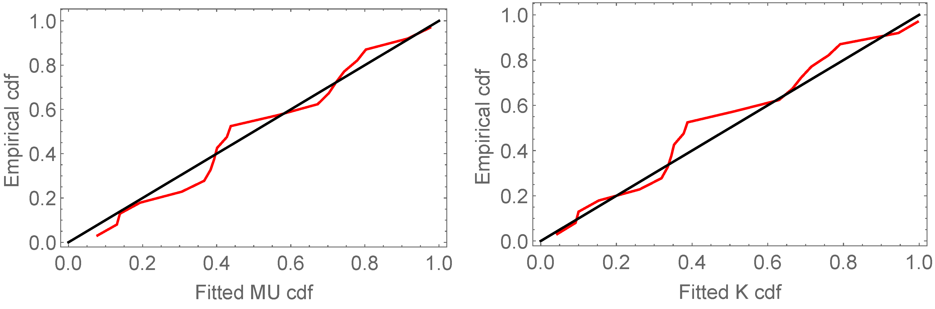
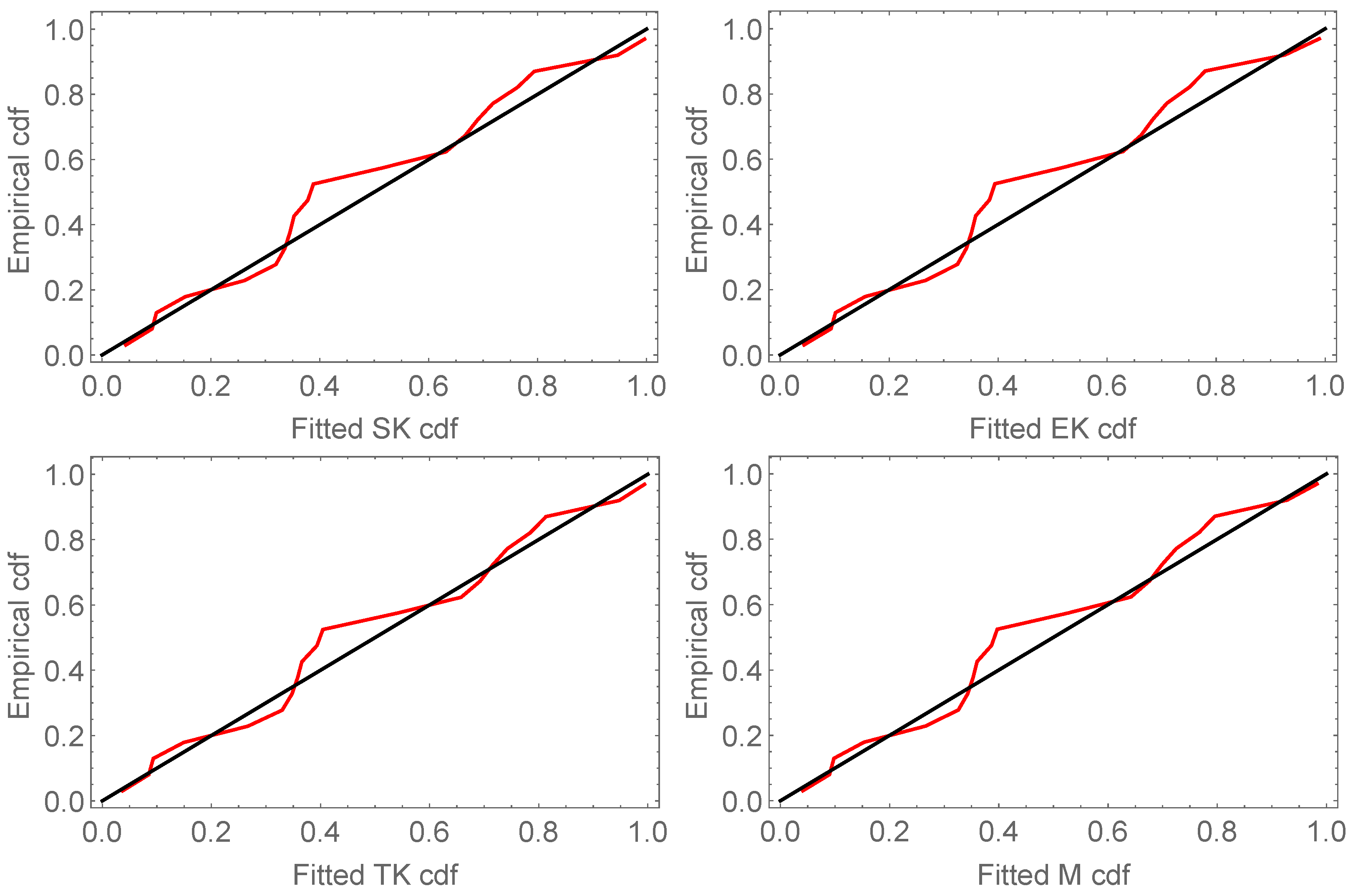
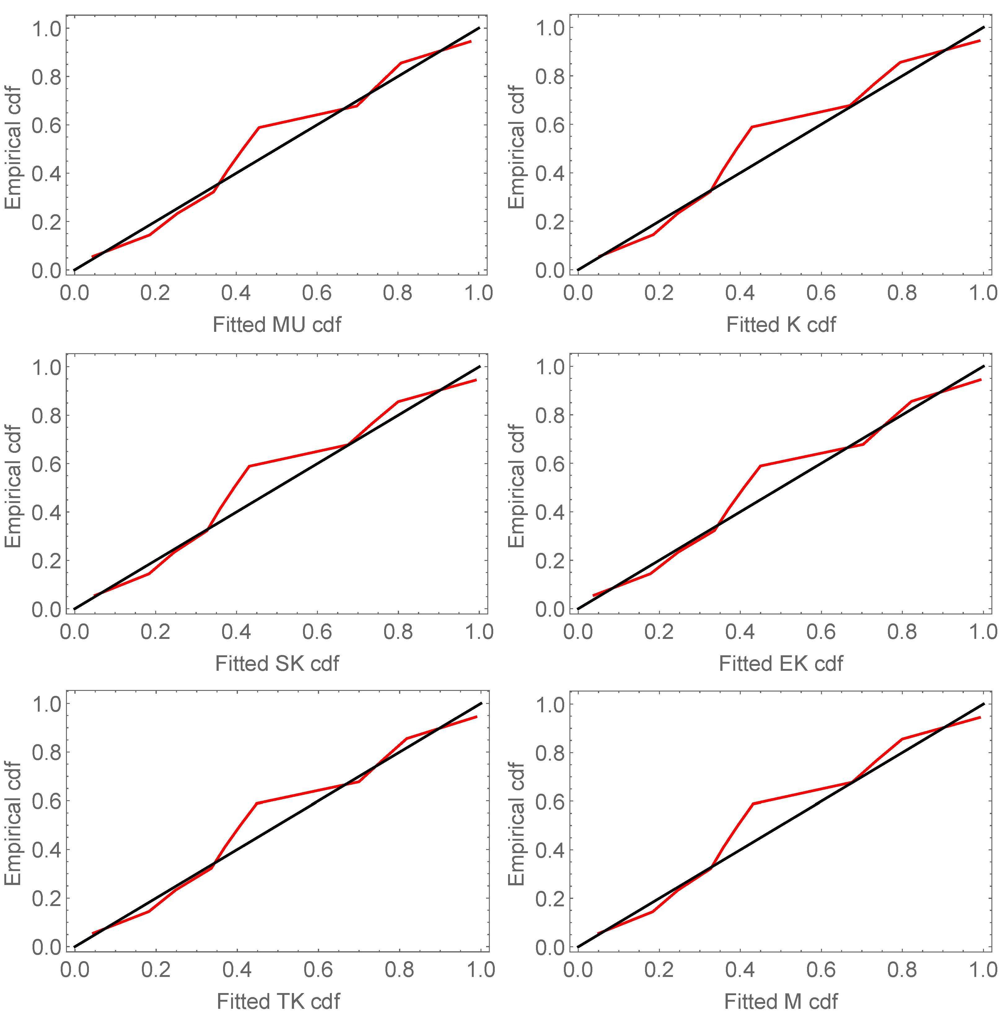
The probability–probability (P-P) plots of the fitted models for the two data sets are shown in Figure 4 and Figure 5. It can be observed that the MU model achieves a better approximation between the empirical and theoretical curves and provides a better fit than other models.

Figure 4. The P-P plots of the proposed model and other compared models for the first data set.

Figure 5. The P-P plots of the proposed model and other compared models for the second data set.

9. Conclusions and Perspectives

In this article, a new family of distributions, called the “modified GG” (MGG) family, is proposed. It provides some generated families and new flexible modified distributions whose probability density and hazard function shapes are desirable for numerous modeling purposes. The proposed MGG family has some interesting characteristics, such as providing more flexible models without adding any additional parameters. We study a special model, namely the modified uniform (MU) distribution, in detail. Various estimation methods of the MU model are studied and assessed using a simulation study. An analysis of two real data sets indicates that the MU distribution can be efficiently used for modeling data arising from different real-life situations. The MU distribution may attract wider applications in many applied areas such as engineering, quality control, medicine, and agriculture, among others, to model different real-life data sets.

The perspectives of this study are numerous, including more developments based on the novel power-exponential transformation approach (with the bivariate case being of particular interest), the applications of introduced lifetime sub-distributions of the MGG family, and the construction of quantile regression models by exploiting the flexibility of the MU distribution.

References

- Marshall, A.N.; Olkin, I. A new method for adding a parameter to a family of distributions with applications to the exponential and Weibull families. Biometrika 1997, 84, 641–652. [Google Scholar] [CrossRef]
- Gillariose, J.; Tomy, L.; Chesneau, C.; Jose, M. Recent developments in Marshall-Olkin distributions. Contrib. Math. 2020, 2, 71–75. [Google Scholar]
- Eugene, N.; Lee, C.; Famoye, F. Beta-normal distribution and its applications. Commun. Stat.-Theory Methods 2002, 31, 497–512. [Google Scholar] [CrossRef]
- Gómez-Déniz, E.; Sarabia, J.M. A Family of Generalised Beta Distributions: Properties and Applications. Ann. Data Sci. 2018, 5, 401–420. [Google Scholar] [CrossRef]
- Gupta, R.C.; Gupta, P.L.; Gupta, R.D. Modeling failure time data by Lehman alternatives. Commun. Stat.-Theory Methods 1999, 27, 887–904. [Google Scholar] [CrossRef]
- Barreto-Souza, W.; Simas, A. The exp-G family of probability distributions. Braz. J. Probab. Stat. 2013, 27, 84–109. [Google Scholar] [CrossRef]
- Kumaraswamy, P.A. Generalized probability density function for double bounded random processes. J. Hydrol. 1980, 46, 79–88. [Google Scholar] [CrossRef]
- Cordeiro, G.M.; de Castro, M. A new family of generalized distributions. J. Stat. Comput. Simul. 2011, 81, 883–898. [Google Scholar] [CrossRef]
- Chesneau, C.; Bakouch, H.S.; Sharma, V. A new family of distributions based on a poly-exponential transformation. J. Test. Eval. 2019, 8, 289–307. [Google Scholar] [CrossRef]
- Souza, L.; Júnior, W.R.O.; Brito, C.C.R.; Chesneau, C.; Ferreira, T.A.E.; Soares, L.G.M. On the sin-G class of distributions: Theory, model and application. J. Math. Model. 2019, 7, 357–379. [Google Scholar]
- Taketomi, N.; Yamamoto, K.; Chesneau, C.; Emura, T. Parametric distributions for survival and reliability analyses, a review and historical sketch. Mathematics 2022, 10, 3907. [Google Scholar] [CrossRef]
- Swain, J.; Venkatraman, S.; Wilson, J.R. Least squares estimation of distribution function in Johnsons translation system. J. Stat. Comput. Simul. 1988, 29, 271–297. [Google Scholar] [CrossRef]
- Gupta, R.D.; Kundu, D. Generalized exponential distribution: Different method of estimations. J. Stat. Comput. Simul. 2001, 69, 315–337. [Google Scholar] [CrossRef]
- Cheng, R.C.H.; Amin, N.A.K. Estimating parameters in continuous univariate distributions with a shifted origin. J. R. Stat. Soc. Ser. B (Methodol.) 1983, 45, 394–403. [Google Scholar] [CrossRef]
- Choi, K.; Bulgren, W. An estimation procedure for mixtures of distributions. J. R. Stat. Soc. Ser. B (Methodol.) 1968, 30, 444–460. [Google Scholar] [CrossRef]
- Boos, D.D. Minimum distance estimates for location and goodness of fit. J. Am. Stat. Assoc. 1981, 76, 663–670. [Google Scholar] [CrossRef]
- Anderson, T.W.; Darling, D.A. Asymptotic theory of certain “goodness of fit” criteria based on stochastic processes. Ann. Math. Stat. 1952, 23, 193–212. [Google Scholar] [CrossRef]
- Anderson, T.W.; Darling, D.A. A test of goodness of fit. J. Am. Stat. Assoc. 1954, 49, 765–769. [Google Scholar] [CrossRef]
- Luceno, A. Fitting the generalized Pareto distribution to data using maximum goodness-of-fit estimators. Comput. Stat. Data Anal. 2006, 51, 904–917. [Google Scholar] [CrossRef]
- Sharma, D.; Chakrabarty, T.K. On size biased Kumaraswamy distribution. Stat. Optim. Inf. Comput. 2016, 4, 252–264. [Google Scholar] [CrossRef]
- Lemonte, A.J.; Souza, W.B.; Cordeiro, G.M. The exponentiated Kumaraswamy distribution and its log-transform. Braz. J. Probab. Stat. 2013, 27, 31–53. [Google Scholar] [CrossRef]
- Shuaib, K.M.; Robert, K.; Lena, H.I. Transmuted Kumaraswamy distribution. Stat. Transit. New Ser. 2016, 17, 183–210. [Google Scholar]
- McDonald, J.B. Some generalized function for the size distributions of income. Econometrica 1984, 52, 647–663. [Google Scholar] [CrossRef]
- Murthy, D.N.P.; Xie, M.; Jiang, R. Weibull Models, Wiley Series in Probability and Statistics; John Wiley and Sons: New York, NY, USA, 2004. [Google Scholar]
- Stoop, B.T.J.; Ouden, G.D. Diffusion of Silicon Nitride to Austenitic Stainless Steel without Interlayers. Metall. Mater. Trans. A 1993, 24, 1835–1843. [Google Scholar] [CrossRef]
- Wang, X.; Yu, C.; Li, Y. A new finite interval lifetime distribution model for fitting bathtub-shaped failure rate curve. Math. Probl. Eng. 2015, 2015, 1–6. [Google Scholar] [CrossRef]
- Shama, M.S.; Dey, S.; Altun, E.; Afify, A.Z. The gamma–Gompertz distribution: Theory and applications. Math. Comput. Simul. 2022, 193, 689–712. [Google Scholar] [CrossRef]
Disclaimer/Publisher’s Note: The statements, opinions and data contained in all publications are solely those of the individual author(s) and contributor(s) and not of MDPI and/or the editor(s). MDPI and/or the editor(s) disclaim responsibility for any injury to people or property resulting from any ideas, methods, instructions or products referred to in the content. |
© 2023 by the authors. Licensee MDPI, Basel, Switzerland. This article is an open access article distributed under the terms and conditions of the Creative Commons Attribution (CC BY) license (https://creativecommons.org/licenses/by/4.0/).