
Modified Padé–Borel Summation

Materialica + Research Group, Bathurst St. 3000, Apt. 606, Toronto, ON M6B 3B4, Canada
Axioms 2023, 12(1), 50; https://doi.org/10.3390/axioms12010050
Submission received: 17 November 2022
/
Revised: 26 December 2022
/
Accepted: 27 December 2022
/
Published: 3 January 2023
(This article belongs to the Special Issue Mathematical Analysis and Applications III)
Abstract
We revisit the problem of calculating amplitude at infinity for the class of functions with power-law behavior at infinity by means of a resummation procedure based on the truncated series for small variables. Iterative Borel summation is applied by employing Padé approximants of the “odd” and “even” types modified to satisfy the power-law. The odd approximations are conventional and are asymptotically equivalent with an odd number of terms in the truncated series. Even approximants are new, and they are constructed based on the idea of corrected approximants. They are asymptotically equivalent to the even number of terms in truncated series. Odd- and even-modified Padé approximants could be applied with and without a Borel transformation. The four methods are applied to some basic examples from condensed matter physics. We found that modified Padé–Borel summation works well in the case of zero-dimensional field theory with fast-growing coefficients and for similar examples. Remarkably, the methodology of modified Padé–Borel summation appears to be extendible to the instances with slow decay or non-monotonous behavior. In such situations, exemplified by the problem of Bose condensation temperature shift, the results are still very good.
Keywords:
modified Padé-Borel summation; odd and even Padé approximants; iterative Borel summation and modified Padé approximantsMSC:
90C59; 2B80; 81T15; 80M35; 80M50; 40G10; 40G991. Brief Introduction to Odd and Even Modified Padé Approximants
The simplest, most transparent and widely accepted way to extrapolate power series is to apply the Padé approximants , which are represented as the ratio of two polynomials of the order n and m, respectively. The coefficients of are derived directly from the coefficients of the given power series [1,2]. They follow from the requirement of asymptotic equivalence to the given series of the function . When it is necessary to emphasize the former point, we write simply .
Among rational approximations, the Padé approximants locally are the best rational approximations of the power series. They also may have poles which are used to determine singularities [1,2,3]. In our problems, we will try to avoid approximants with poles in finite domains.
Thus, among the Padé approximations, we select only such approximants which are holomorphic functions. It is established rigorously by Gonchar that the holomorphy of diagonal Padé approximants in a given domain implies their uniform convergence inside this domain [4]. Thus, for the problems with a finite number of terms in the expansion, we will try to restrict the sets of Padé approximants only to the diagonal sequences and find such groupings of approximants with clear numerical convergence.
It always makes sense before considering more sophisticated approximations to attempt to apply well-developed techniques of Padé approximants. It is also highly desirable to develop some modified Padé approximants to capture the class of functions with power-law behavior at infinity, since standard Padé approximations are obviously limited in such respect by the integer powers (see also [5]). Consider only non-negative functions with asymptotic behavior
at infinity with known index at infinity and unknown amplitude at infinity A. The following expansion at small x,
is given as well. Here, N is integer and . Let us calculate the amplitude at infinity A based on the truncation (2) and known index .
Usually, only the case of odd is studied [6,7,8]. In such an approach, one has to apply the transformation
to the truncated series in order to get rid of the power-law behavior at infinity. Applying the well-known technique of diagonal Padé approximants to the function , one can readily obtain the sequence of approximations for the amplitude at infinity [6],
where is a non-negative integer. Thus, the following modified Padé quasi-rational approximant
is defined for odd cases. The approximants evolve with increasing n and the amplitudes follow. The amplitudes in the subsequent approximations are not formally related.
The even case of requires special attention and is rarely (never?) considered explicitly with Padé approximants. While for the very long truncations, the difference between odd and even cases may be insignificant and ignored, for short truncations, the difference can very well be detectable. Of course, to avoid the problem of odd–even approximants altogether, one can resort to the self-similar iterated roots, which assimilate the coefficients one-by-one [9]. However, in contrast, the Padé approximants can be easily and routinely extended to very high orders.
Below, we suggest a way to apply Padé techniques for even numbers of terms in the truncation. Instead of meekly increasing the order of approximation, one can adopt the idea of corrected approximants [10]. In an such approach, to find the amplitude A, we divide the original series for by the “corrector” and find the new truncated series
The corrector is supposed to have a correct power-law behavior at infinity and be the same for all n. It also defines some fixed contribution to the amplitude. The function and Padé approximants will be designed to contribute only to the amplitude, producing a correction to it.
Thus, in the case of even , we ensure the correct index already in the starting approximation once and for all n. In place of , one can assume the simplest, modified-odd Padé approximant, i.e.,
One can find a corresponding value for the amplitude
Then, one can apply rational approximants to the series and build a sequence of the even diagonal Padé approximants asymptotically equivalent to . The sought amplitude at infinity can be found as follows
where , is a positive integer. Thus, the following modified-even Padé approximant
is defined for even case. The sought solution is factorized. The first factor is represented by a modified a quasi-rational Padé approximation of the lowest order, ensuring the correct index at infinity, and the second factor is also a diagonal Padé approximant, characterizing the rational part of the solution. In the current paper, there are two novel features:
(1) Novel, modified-even Padé approximants based on the even number of terms in truncations are advanced and applied.
(2) Odd-modified and even-modified Padé approximants are advanced and applied in conjunction with an iterative Borel summation.
The methodology of modified Padé–Borel summation is very user-friendly and always leads to a unique solution. In addition, the convergence of the method is controlled by the general theorem of Gonchar [4]. We recommend that various modified Padé and Padé–Borel techniques are to be tried whenever the perturbative problems of finding the amplitude at infinity are studied.
The modified Padé–Borel summation takes into account an arbitrary power-law behavior at infinity, making it superior to the standard Padé–Borel approach which considers only integer powers. In addition, the approach is much simpler compared with optimal Borel–Leroy, Mittag–Leffler and iterative Borel techniques [9,11], allowing us to go easily to very high orders of perturbation theory.
2. Modified Padé Approximants and Iterative Borel Summation
Borel summation is applied for the effective summation of the functions with known truncation at small x [9,11,12,13,14,15,16,17,18,19,20]. More references on Borel summation can be found in our recent paper [11].
The Borel summation can be applied also to the hypergeometric functions/ approximants [21,22]. Such a technique leads to the hypergeometric-Meijer approximants [23,24]. Yet, such techniques are rather cumbersome. The non-uniqueness of the approximants complicates establishing explicitly the property of asymptotic equivalence with the truncated series. Their application also requires a fitting procedure [25,26]. As a consequence, the results appear only in numerical form. Therefore, a much simpler method of Padé approximant should not be abandoned; see also [27]. Our choice throughout the current paper of the modified Padé approximants allows for analytical calculation of the amplitudes while keeping the calculations rather simple and straightforward. Again, just like in the paper [9], we can extend the technique from the amplitude A calculations to the indices .
The iterative Borel summation starts with the transformation of the truncated series (2) to the form
which is defined following [13]. In the current paper, we are concerned only with the discrete case of positive integer b, standing for the number of iterations. The transform is meant to capture the case when grows as (see [9,13,14]).
Our goal now is to accomplish an inverse transformation returning to the original truncated series. Ultimately, the truncation (6) ought to be extended to all for the inverse transformation to become feasible. Such an extension is made either by means of Padé approximants [15,16,17,18,19] or by adding the information on large-n asymptotics of [14]. However, the whole table of the Padé approximants is not able to capture the power-law (1) with arbitrary , and it is used for extrapolation to finite values of variable x. With the power-law condition (1) imposed at infinity, the series can be summed by means of modified Padé approximants of the odd and even -types.
Assume once again that we know the value of the index . The modified Padé approximants of the and -types, at large x, behave as
As a result, the large-variable behavior of the reconstructed function acquires the form
with the amplitude
Consider first the case of odd , and let us calculate the marginal amplitude in the odd case. To this end, let us apply the now familiar transformation (3) to the truncated series . In such a way, we arrive to the transformed series
getting rid of the power-law behavior at infinity, at least formally. Applying now the well-known technique of modified-odd Padé approximants equivalent asymptotically to , one can find the sequence of approximations for the marginal amplitude,
where is a non-negative integer, and .
Consider now the case of even . Just as in the case of now familiar modified-even Padé approximants, let us ensure the correct index already in the starting approximation . In place of , one can assume the simplest Padé approximant with a correct form at infinity,
Then, one can find the corresponding values for the amplitude
Instead of increasing the order of approximation, one can again adopt the idea of corrected approximants [10]. In such an approach, to find the correction to the amplitude , we divide the original Borel-transformed series by the corrector and find yet new truncated series
Finally, we have to build a sequence of the diagonal Padé approximants asymptotically equivalent to . The marginal amplitude could be found as a product
where , is a positive integer, and .
Obviously, the complete amplitude can be found as well,
in the same form for odd and even cases, notwithstanding.
In the discrete case of positive integer b, we consider only the sequences of averages with the smallest b so that the sought amplitudes are given as follows,
in the same form for odd and even cases [9].
Let us consider the very popular in field theory and statistical mechanics, zero-dimensional anharmonic model represented by the integral
with the non-negative coupling parameter g. Expansion in powers of g leads to the strongly divergent series with the coefficients The strong-coupling form of the integral is a power-law
Using the methods described above for defining the large-variable amplitudes for the modified Padé approximations of different sorts, we obtain the results illustrated in Figure 1, Figure 2, Figure 3 and Figure 4.
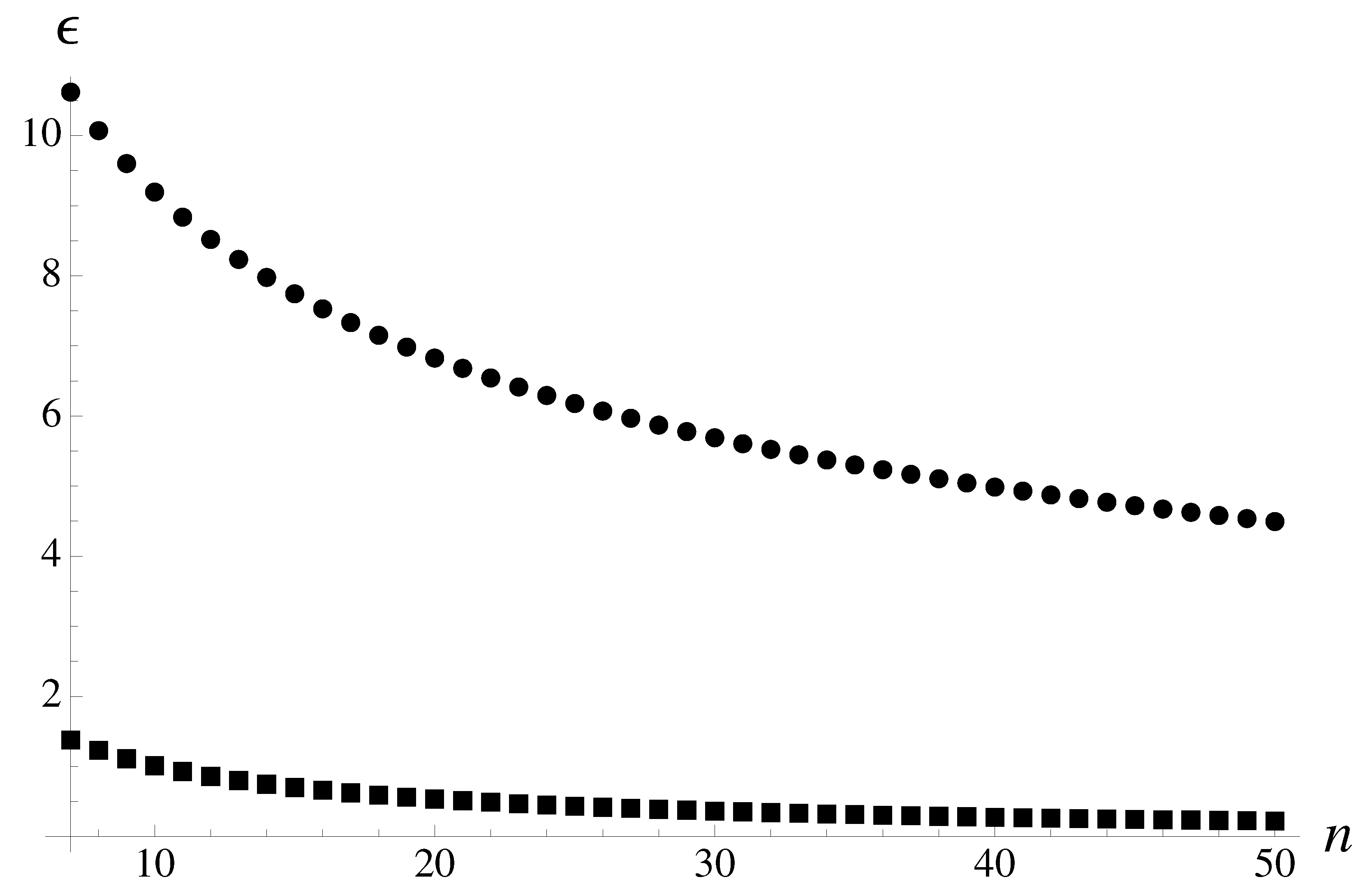
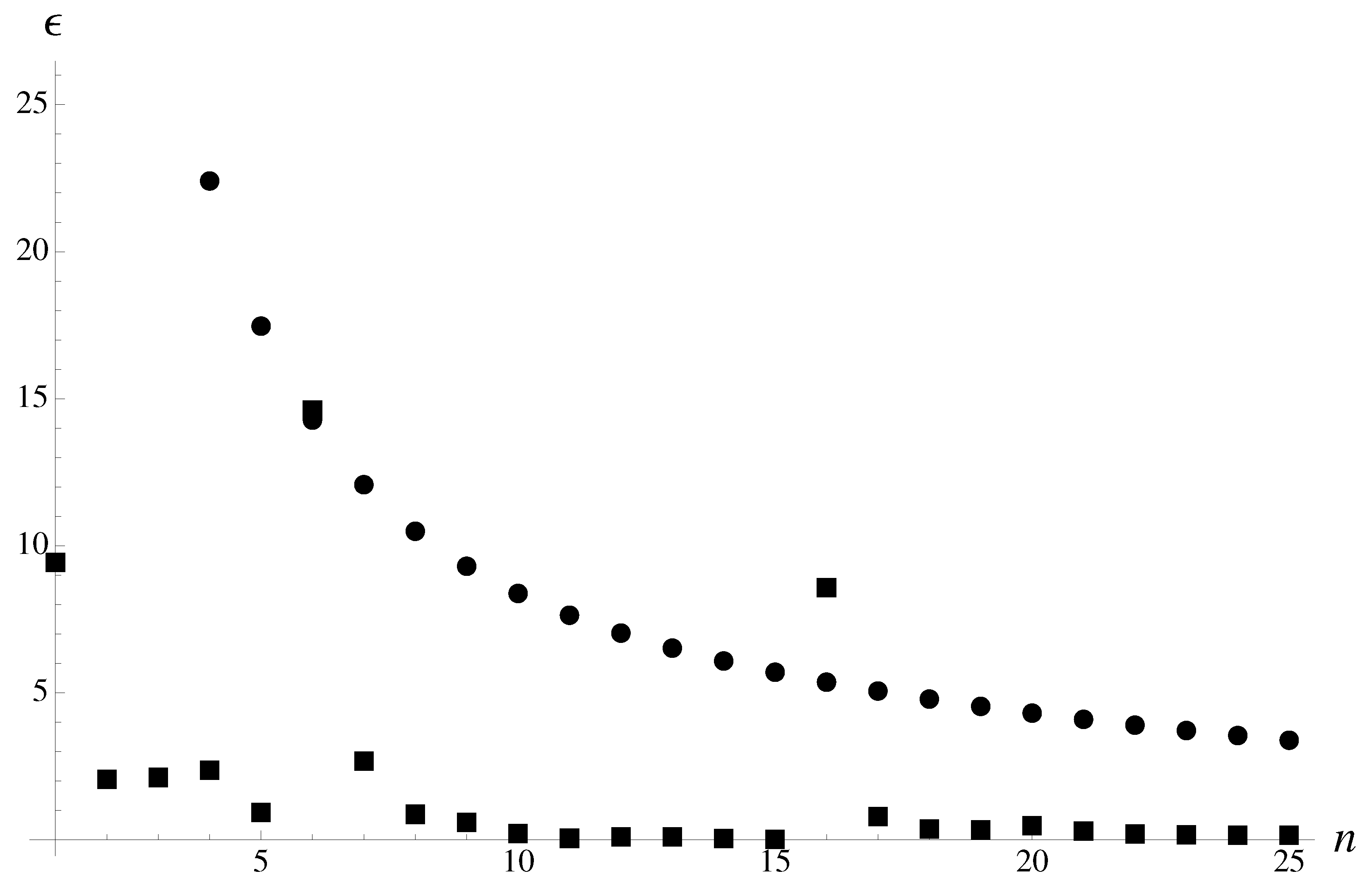
In Figure 1, the relative percentage error for the amplitude is shown, which is dependent on the approximation number n. It is presented for the modified-odd Padé approximants with disks and is shown with squares for modified-odd Padé-Borel summation. Only a single-iteration step is made. In the latter case, performance appears to be better by an order of magnitude compared with standard modified-odd Padé approximants.
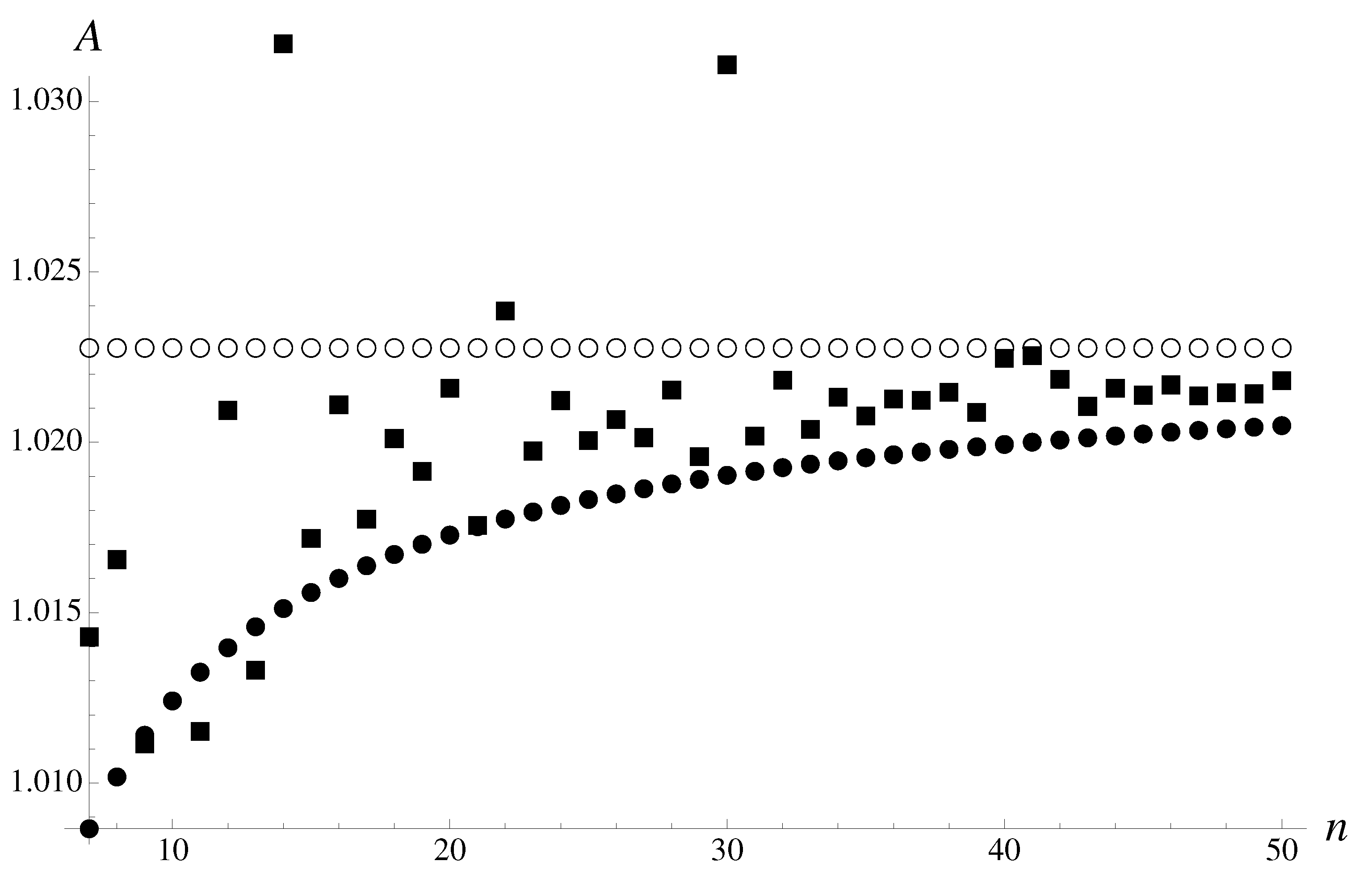
The results of modified-odd Padé–Borel summation results are very good, with a relative percentage error of 0.1–0.2%, as shown in Figure 2. The amplitude obtained with the modified-odd Padé–Borel summation performed in a single-iteration step is shown with disks, and it is dependent on the approximation number n. The amplitude for the modified-odd Padé–Borel summation performed in two-iteration steps is shown with squares. The exact result, , is shown for comparison with (empty) circles.
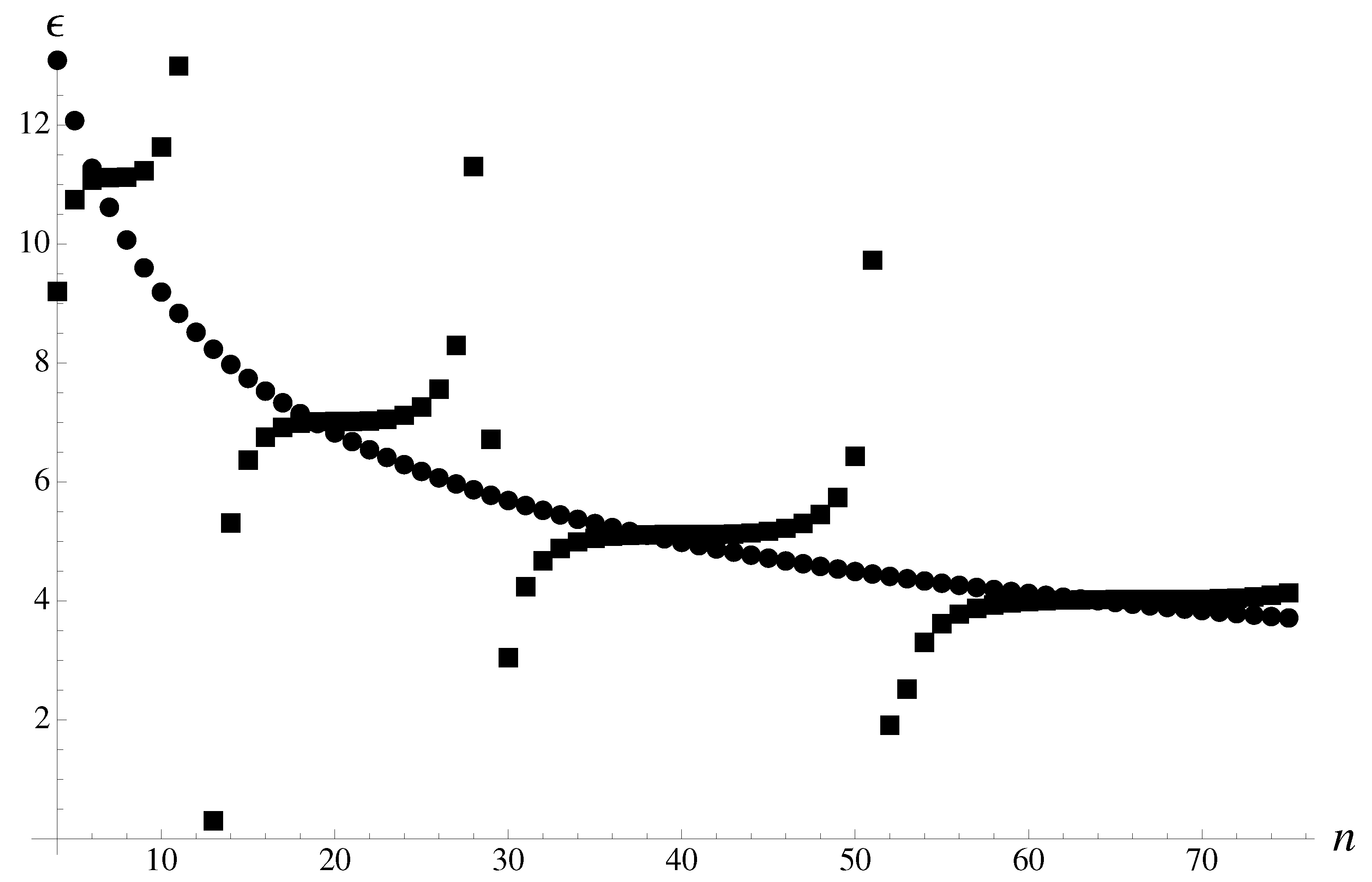
In Figure 3, the relative percentage error for the amplitude is shown for the modified-odd and modified-even Padé approximants, and it is dependent on the approximation number n. The results obtained with the modified-odd Padé approximants are shown with disks, while the relative percentage error for modified-even Padé summation is shown with squares. The latter, even approximants demonstrate striking quasi-periodic performance with error possessing minima at some quasi-periodic intervals, which is in contrast with a monotonous improvement with n in the case of odd approximants. Already, the first minimum gives the best result, implying that the higher-order are somewhat redundant. We see that performance of odd and even approximants can be very different, and modified-even approximants can outperform the odd, in principle.
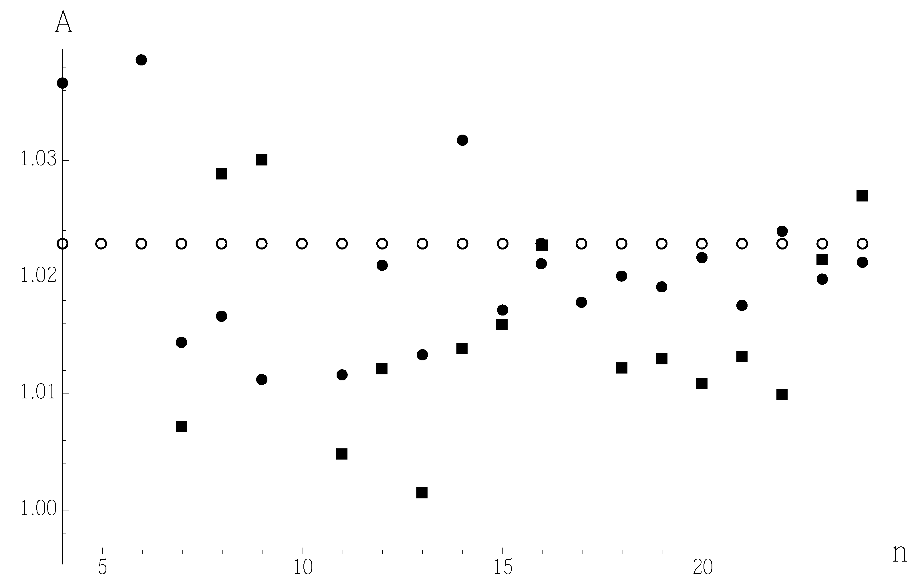
In Figure 4, performances of modified-odd and modified-even Padé–Borel approximations in a two-step iteration procedure are compared. For the modified-odd Padé–Borel summation performed in two-iteration steps, the amplitude is shown with disks, and it is dependent on the approximation number n. The approximation for the modified-even Padé–Borel summation performed in two-iteration steps is shown with squares. The performances appear to be similar, and rather good, but odd approximations are more stable and can be extended to higher orders than even.
3. Examples
Realistic problems to be discussed below are more complicated than the model example discussed above. In many realistic problems, only very short truncations are available. In addition, the coefficients do not show the same perfect growth pattern and may be even slowly decaying or irregular. Nevertheless, the features observed in the model case appear to be robust and persist to the imperfect realistic physical cases.
For the short truncations, it makes sense to try to use all available for odd or even N in the expansion (2), and a certain gain can be reached just by technical means, without computing more coefficients.
3.1. Cusp Anomalous Dimension
In the supersymmetric Yang–Mills theory, in the limit of a large angle, the planar cusp anomalous dimension is linear in angle, with a coefficient , that is the cusp anomalous dimension of a light-like Wilson loop, which depends only on the coupling g. The weak-coupling and strong-coupling expansions are available for the sought quantity (see [28,29] and references therein).
In terms of the variable , after minor transformations, the problem can be recast into the familiar form (2) with for the function with
and in the strong-coupling limit of (1), takes the form of a power-law
with and . Let us estimate the amplitude at large x by various modified Padé approximations. In such cases, only odd approximations can exploit all terms from the weak-coupling expansion.
Standard modified-odd Padé approximants give with all terms from the weak-coupling exploited. Meanwhile, modified-even Padé approximants give with only two non-trivial terms from the weak-coupling expansion being used.
Modified-odd Padé approximation when combined with the Borel summation gives the best result in one-step, , with an accuracy of 3%. Even Padé approximation when combined with the Borel summation gives only with abysmal accuracy.
Thus, compared with conventional odd Padé approximants, modified-odd Padé approximation applied for Borel summation brings a significant improvement. Yet, the best result, , is achieved by the optimal Borel–Leroy summation [11]. However, such a technique is considerably more sophisticated compared with a direct application of modified Padé–Borel summation.
3.2. Two-Dimensional Polymer
It is forbidden for the polymer segments to occupy the same space. As a consequence, there is a swelling effect in the typical polymer chain radius when compared to the non-perturbed segments. The swelling could be measured by the swelling factor where g stands for the dimensionless coupling parameter [30]. As , the swelling factor behaves as a power-law, i.e.,
The index at infinity is considered to be known exactly, [31,32].
For the swelling factor, perturbation theory yields the expansion in powers of the dimensionless coupling parameter [30]. Consider the two-dimensional polymer coil [30] with
as .
Let us estimate the amplitude at infinity by various modified Padé approximations. Only even approximations can exploit all terms from the weak-coupling expansion. Standard modified-odd Padé approximants give only with a non-trivial three terms from the weak-coupling exploited. Meanwhile, modified-even Padé approximants give
with all four non-trivial terms from the weak-coupling expansion being used.
Modified-odd Padé approximation combined with the Borel summation gives the result in one-step summation. Modified-even Padé approximation when combined with the Borel summation gives
with reasonably good lower and upper bounds for the amplitude,
The simple average over all four Padé-type estimates imply
and is compatible with the bounds. The true value of amplitude A for the two-dimensional polymer is not known, and our result could be viewed as a prediction. The value of found by the optimal Borel–Leroy summation [11] appears to be close to the lower bound. Current estimates are systematically higher than our previous results obtianed by various approximants in the book [33].
3.3. Bose Condensation Temperature
Introducing interactions to uniform Bose gas leads to a shift of the ideal Bose gas transition temperature to the value of . The shift is considered to depend linearly on the parameter , so that
Here, is the atomic scattering length, and stands for gas density.
The goal is to find theoretically. To this end, the coefficient can be understood formally [34,35,36] as the limit
where g is the effective coupling parameter. However, for the function , one can only find the expansion
as . The modified-odd Padé-summation practically fails after resummation in the third order of perturbation theory, bringing . In contrast, the modified-even Padé summation gives a very good estimate which is obtained after resummation in the fourth order of perturbation theory.
The problem of finding A by means of a Borel summation is undetermined because of the -functional divergent contribution to the amplitude for in formula (9). Using formula (13), but in application to the inverse series and then taking the inverse as discussed for the indeterminate case in the paper [9], we manage to obtain rather reasonable results for the amplitudes at infinity.
The modified-even Padé–Borel summation gives a very good estimate
which is obtained after resummation in the fourth order of perturbation theory with reasonably good lower and upper bounds for the amplitude,
Mind that Monte Carlo simulations (see [10,37] and multiple references therein), give
The modified-odd Padé–Borel summation also gives a sensible estimate , after resummation in the third order of perturbation theory, with the lower and upper bounds, .
The results obtained above by the two modified-even Padé methods and modified-odd Padé–Borel summation well agree with Monte Carlo simulations, and they appear to be close to the estimate obtained by the optimal Mittag–Leffler summation [11].
In the same way, one can find the values of for the field theory [35]. The following formally obtained expansion is available for small g,
It is considered as an input for calculating as .
The modified-even Padé summation again gives a good estimate after resummation in the fourth order of perturbation theory. However, the modified-odd Padé summation fails again, bringing .
The modified-even Padé–Borel summation gives a very good estimate
after resummation in the fourth order of perturbation theory with reasonably good bounds . The results for the amplitude agree quite well with Monte Carlo numerical estimate (see [10] and references therein).
The modified-odd Padé–Borel summation also gives rather sensible estimate , after resummation in the third order of perturbation theory with reasonable bounds for the amplitude, . The result of Mittag–Leffler optimal summation from [11] appears to be close to various modified Padé–Borel summations.
For the field theory, analogous computations can be accomplished. The expansion for as can be found in [35], so that
The modified-odd Padé-summation fails once again, bringing the estimate .
The modified-even Padé summation once again gives a good estimate after resummation in the fourth order of perturbation theory. The modified-even Padé–Borel summation gives a very good estimate
obtained after resummation in the fourth order of perturbation theory with reasonably good bounds . The modified-even Padé–Borel approximation agrees very well with Monte Carlo numerical estimate as discussed in [10].
The modified-odd Padé–Borel summation also gives quite sensible estimate , after resummation in the third order of perturbation theory with reasonable lower and upper bounds, . The result of Mittag–Leffler optimal summation from [11], appears to be close to various modified Padé–Borel summations. The modified-even Padé–Borel summation appears to be in a better agreement with Monte Carlo simulations than the other “Borelian” methods of [9,11].
Remarkably, a rather simple modified-even Padé summation appears to be accurate enough in all three cases considered above. It is the most simple and direct method of estimating the shift, bringing better estimates than obtained before by the method of corrected approximants [10].
3.4. Bose Condensate in Spherical Trap
The wave function of the Bose-condensed atoms in a spherically symmetric harmonic trap can be found from the three-dimensional stationary nonlinear Schrödinger equation [38]. The problem can be reduced to studying only the radial part of the condensate wave function. In terms of the coupling c measuring the intensity/depth of the trap, the ground state energy E of the trapped Bose-condensate can be approximated by the following truncations
and by the power-law
with the amplitude at infinity [38].
The modified-even Padé summation gives a good estimate for the amplitude, after resummation in the fourth order of perturbation theory. The modified-odd Padé summation brings a slightly inferior number but after resummation in the third order of perturbation theory.
The modified-even Padé–Borel summation gives the following estimate
after resummation in the fourth order of perturbation theory with reasonable lower and upper bounds, . The best estimates in this case could be obtained from the conventional sequence of “accuracy-through-order” approximations [1],
with the estimate for the amplitude by their average
The modified-odd Padé–Borel summation also produces a sensible estimate , after resummation in the third order of perturbation theory, with reasonable lower and upper bounds on the amplitude, . The best estimates in this case could be obtained again from the conventional sequence of “accuracy-through-order” approximations,
leading to the estimate for the amplitude by their average
Optimal Mittag–Leffler summation [11] in the fourth-order of perturbation theory produces three close estimates for the amplitude,
with average result . The latter estimate is close to the best results obtained above by modified Padé–Borel summations. In addition, a significant improvement is achieved over the results of optimization through the self-similar power transformation [39].
4. Comments
Our first comment is on the subject of calculating the index at infinity . In the course of such calculations with the strongly divergent series, it makes sense to avoid the diff-log (or, equivalently, ) [20] transformation altogether. The transformation makes the Borel resummation more difficult because in the expression for indices in the Borel technique, there is now a pole [9,11,20]. Such a pole is of the very same nature as in the case of formula (9). It is possible though to escape the problem altogether and develop the Borel techniques without poles.
To such an end, even without a differentiation, the simpler, Padé approximants can be advanced. The index in such an approach can be expressed as follows,
After resummation, the sought function acquires the following form:
where the parameter is always positive. For , the index function is supposed to satisfy the limit
The value of gives the sought index.
We can also use the known asymptotic form (and of ) at small g to express as a truncated power series. For small g, we have to deal with the form
with the RHS expanded in powers of g around the value of . Now, for , we can construct the diagonal Padé approximants
which are always defined as even approximants. Their corresponding limits can be found with relative ease, so that
for all non-negative integers n. The choice of simplifies computations. It corresponds to . Thus, we arrive at the estimates for the index dependent on the approximation number with the terms from the expansion for being employed,
The Borel transform can be applied to the truncated series (23) so that
The diagonal Padé approximant required for calculations at large g behaves as
and the index dependence on n
can be calculated for all non-negative integers n. There is no pole in the formulas of the type of (9), which is reduced to formula (27).
Consider the now familiar integral , given by formula (14), with known exact index . Calculation of the index according to the Padé approximation (24) demonstrates a monotonous convergence, as shown in Figure 5.
Since the index function is strongly divergent at small g, one can hope that application of the Padé–Borel summation directly to can help to improve the convergence of the sequences for the index . Indeed, the Padé–Borel summation according to the formula (27) results in much better numbers, as shown in Figure 5.
We conclude that it is feasible to (1) avoid the singularity in the expression of the type of (9), in the Padé–Borel summation and (2) find a sizable improvement in performance by applying formula (27) instead of formula (24) for calculation of the indices at infinity. Our second comment is on the subject of calculating the amplitude at infinity for a very short series, with in the general expression (2). Quite often, such minimal meaningful truncations are all that is known. Mind that the cost of finding more coefficients could be prohibitive.
In such a case, one can try a special choice of the correcting function , or in the formulas for even approximants, which would not consume in the process of its construction any terms from the already short expansions. In particular, one can try the corrector , where
As , one can see that , automatically satisfying the strong-coupling limit.
In particular, such an approach makes sense for the ground-state energy E of the Schwinger model. In such a case with , only the minimal expansion in the dimensionless coupling parameter x is available. The expansion at small-x for the ground-state energy, as well as multiple references, can be found in the papers [13,29]. The large-x limit is a power-law
All four modified Padé methods of the current paper, applied in a standard way, do not give very good results, with the best number for the amplitude at infinity.
However, by applying the modified-even Padé–Borel technique with the corrector given by formula (28), we find a much better result . Furthermore, without adding any new terms in the expansions for , one can formally apply the same method in higher orders and find The latter result is close to our best estimate from [29].
The form (28) hints that it could be feasible to combine the technique of Borel summation with fractional calculus [7,8]. We would like to introduce fractional derivatives in such a way that a nice asymptotic property of asymptotic scale invariance [9] given by the expression (1) is preserved. To this end, one might look at the generalized Borel formulae of [16] and attempt to extend the class of modified derivatives entering the formulas to fractional derivatives while preserving the asymptotic scaling. Determining the order of fractional derivatives to be employed can be challenging but also productive, since it can be required to be determined uniquely from the optimization conditions of the types used in [9,11].
Fractional modeling can be useful when the information on the sought function is given in the form of data points and complemented by asymptotic exponential decay or by a constant with additive exponential correction asymptotic at infinity. A similar case was discussed in the paper [40]. Spatio-temporal modeling could be performed, in principle, by means of multi-dimensional extensions of the Padé-approximants. The third comment concerns the ground-state energy of the one-dimensional stationary nonlinear Schrödinger equation describing the Bose-condensed atoms in a harmonic trap. The equation was employed to find the wave function of the Bose-condensed atoms in a harmonic trap [41,42]. The expansion for the function in powers of the small effective coupling g was obtained up to in the general expression (2) [41,42].
In the strong-coupling limit, the ground-state energy behaves as a power-law, i.e.,
with [42]. It turns out that modified-odd Padé approximants work well in the fifth order of perturbation theory, giving rather accurate estimates,
Modified-even Padé approximants also work well in fourth order of perturbation theory, giving the estimate
for the amplitude.
However, if we unwittingly apply the Borel summation in such an almost perfect case for the modified Padé approximants, then we can only hope that the result will stray not too far from the already good results achieved by the Padé approximants. Indeed, the modified-odd Padé–Borel summation gives the following estimates
after resummation in the fifth order of perturbation theory. In addition, the modified-even Padé–Borel summation also produces a sensible estimate after resummation in the fourth order of perturbation theory. The estimates appear to be located not too far from the best solutions by the Padé approximants presented above.
5. Discussion and Conclusions
Finally, we discuss the ongoing attempts to apply the techniques developed in the paper to find critical indices for the two popular models of statistical physics where some unresolved issues still exist. In the case of compressibility of hard disks [43,44,45,46], the value of the index is only conjectured. In the case of the susceptibility of the so-called (2 + 1)-dimensional Ising model [32,47,48], the standard methods give results systematically higher than expected. Below, we briefly discuss only the main results, while the complete results will be presented elsewhere.
The equation of state of the fluid of hard discs expresses the so-called compressibility factor Z as the function of packing fraction f [43,44]. The compressibility factor exhibits a divergent, power-law behavior at the filling and
with the unknown critical index . For low density, the compressibility factor could be expressed as an expansion in powers of f, and the nine terms of the perturbative expansion are available [45,46]. When the critical point is finite, the transformation
could be applied to bring the problem to the generic form considered throughout the current paper. Following the same idea as in paper [9], and performing the diff-log transformation and taklng its inverse when required [9], the critical index can be calculated as the specific amplitude.
Standard modified-odd Padé approximants give , with all possible terms from the expansion exploited. The modified-even Padé approximants give with all terms from the perturbative expansion being used. Such estimates appear to be rather close to the results of the paper [20].
Modified-odd Padé approximation when combined with the Borel summation gives . Modified even Padé approximants when combined with the Borel summation give a close result . These values are much closer to the conjectured value of [43,44] than the result from the paper [20]. Let us also discuss the problem of finding the critical index for susceptibility of the (2 + 1)-dimensional Ising model on the square lattice [47]. The susceptibility [47], expressed as the function of an inverse temperature x diverges at a critical point as a power-law
with the critical index [32,47,48]. The high-temperature expansion of the susceptibility on a square lattice is available up to the terms of 16th order in the variable x [47]. It is believed that the (2 + 1) and three-dimensional isotropic Ising model [32] belong to the same universality class, but the conclusion appears to be poorly supported by the resummation results for the (2 + 1)-dimensional Ising model [47].
The methodology of the papers [9,20] can be employed to compute the index with various modifications of the Padé approximants introduced in the current paper. Yet, without the Borel transform, the standard modified-odd Padé approximants give , with all terms from the expansion exploited. The modified-even Padé approximants give with all possible terms from the perturbative expansion being used. Such estimates appear to be significantly higher than the result of the paper [47], which is obtained by various advanced resummation techniques.
Modified-odd Padé approximants combined with the Borel summation give . Modified-even Padé approximants when combined with the Borel summation give a slightly lower result, . These values are much closer to the values of [32], and from [48], which were obtained for the three-dimensional isotropic Ising model. Thus, we cautiously confirm that the (2 + 1)-dimensional Ising model on the square lattice suggests the values for the critical index that are close to the currently accepted values for the three-dimensional Ising model.
In summary, in the current paper, we suggest a novel method of modified-even Padé approximants based on the even number of terms in truncations (2). The techniques of known odd-modified and of novel, even-modified Padé approximants are also employed for the iterative Borel summation. Because of their accuracy and simplicity, various modified Padé and Padé–Borel techniques should be tried whenever the problems of finding the amplitude at infinity reconstructions arise.
In order for the powerful general results of Gonchar [4] to be applicable to realistic truncated problems considered in the current paper, the problems should be with reasonable accuracy approximated by the holomorphic, modified Padé approximations. All innovations, transformations, etc. serve the purpose of improving the convergence and accuracy of reasonable numerical approximations. Sometimes, significant gain can be found.
The methodology of modified Padé–Borel summation is much simpler technically than other methods involving optimization, special functions or heavy numerical analysis. Its application always leads to unique solutions, and the convergence of the method is controlled by the general theorem of Gonchar [4]. Compared to the well-known Padé–Borel method, the modified Padé–Borel method could be applied to the case of functions with an arbitrary power-law asymptotic behavior at infinity.
Modified-odd Padé–Borel summation performs well where it is expected; e.g., it works well in the case of zero-dimensional field theory with fast-growing and in the case of cusp anomalous dimension. In the former case, very good results for the amplitude A were previously obtained by the variational perturbation method of Kleinert [49] and by our own self-similar additive approximants [33]. However, such techniques require additional information on the so-called correction-to-scaling critical indices, while the modified-odd Padé–Borel summation works without such knowledge.
Remarkably, the methodology of modified Padé–Borel summation appears to be extendable to the instances with slow decay or non-monotonous behavior of the coefficients . In such situations, exemplified by the Bose condensation temperature shift, the results are still good. The method of modified-even Padé approximants brings the most direct and quite accurate estimates for the shift. It works well compared to other more involved methods, such as Mittag–Leffler, Borel–Leroy and iterative Borel summations employed previously [9,11]. For another important problem of the expansion factor of the two-dimensional polymer modeled as random walks without intersections, the value of critical amplitude is not known, and our results could be viewed as a prediction.
We should also remember that there are important physical problems where all current modified Padé and Padé–Borel schemes fail without any hope to improve them by applying exclusively various rational and quasi-rational approximations. A vivid example could be given by the ground state energy of a one-dimensional Bose gas with contact interactions quantified by the non-dimensional coupling parameter [50,51]. In such case(s), we have to consider irrational approximations along the lines of the papers [9,10].
Funding
This research received no external funding.
Conflicts of Interest
The author declares no conflict of interest.
References
- Baker, G.A.; Graves-Moris, P. Padé Approximants; Cambridge University: Cambridge, UK, 1996. [Google Scholar]
- Suetin, S.P. Padé approximants and efficient analytic continuation of a power series. Russ. Math. Surv. 2002, 57, 43–141. [Google Scholar] [CrossRef]
- Andrianov, I.; Awrejcewicz, J. New trends in asymptotic approaches: Summation and interpolation methods. Appl. Mech. Rev. 2001, 54, 69–92. [Google Scholar] [CrossRef]
- Gonchar, A.A. Rational Approximation of Analytic Functions. Proc. Steklov Inst. Math. 2011, 272 (Suppl. 2), S44–S57. [Google Scholar] [CrossRef]
- Andrianov, I.; Shatrov, A. Padé approximants, their properties, and applications to hydrodynamic problems. Symmetry 2021, 13, 1869. [Google Scholar] [CrossRef]
- Bender, C.M.; Boettcher, S. Determination of f (∞) from the asymptotic series for f (x) about x = 0. J. Math. Phys. 1994, 35, 1914–1921. [Google Scholar] [CrossRef]
- Dhatt, S.; Bhattacharyya, K. Asymptotic response of observables from divergent weak-coupling expansions: A fractional-calculus-assisted Padé technique. Phys. Rev. E 2012, 86, 026711. [Google Scholar] [CrossRef] [PubMed]
- Dhatt, S.; Bhattacharyya, K. Accurate estimates of asymptotic indices via fractional calculus. J. Math. Chem. 2013, 52, 231–239. [Google Scholar] [CrossRef]
- Gluzman, S. Iterative Borel Summation with Self-Similar Iterated Roots. Symmetry 2022, 14, 2094. [Google Scholar] [CrossRef]
- Gluzman, S.; Yukalov, V.I. Self-similarly corrected Padé approximants for indeterminate problem. Eur. Phys. J. Plus 2016, 131, 340–361. [Google Scholar] [CrossRef]
- Gluzman, S. Optimal Mittag-Leffler Summation. Axioms 2022, 11, 202. [Google Scholar] [CrossRef]
- Hardy, G.H. Divergent Series; Clarendon Press: London, UK, 1949. [Google Scholar]
- Bender, C.M.; Orszag, S.A. Advanced Mathematical Methods for Scientists and Engineers. In Asymptotic Methods and Perturbation Theory; Springer: New York, NY, USA, 1999. [Google Scholar]
- Suslov, I.M. Divergent Perturbation Series. J. Exp. Theor. Phys. 2005, 100, 1188–1233. [Google Scholar] [CrossRef][Green Version]
- Sidi, S. Practical Extrapolation Methods; Cambridge University Press: Cambridge, UK, 2003. [Google Scholar]
- Kompaniets, M.V. Prediction of the higher-order terms based on Borel resummation with conformal mapping. J. Phys. Conf. Ser. 2016, 762, 012075. [Google Scholar] [CrossRef]
- Graffi, S.; Grecchi, V.; Simon, B. Borel summability: Application to the anharmonic oscillator. Phys. Lett. B 1970, 32, 631–634. [Google Scholar] [CrossRef]
- Simon, B. Twelve tales in mathematical physics: An expanded Heineman prize lecture. J. Math. Phys. 2022, 63, 021101. [Google Scholar] [CrossRef]
- Antonenko, S.A.; Sokolov, A.I. Critical exponents for a three-dimensional O(n)-symmetric model with n > 3. Phys. Rev. E 1995, 51, 1894–1898. [Google Scholar] [CrossRef]
- Yukalov, V.I.; Gluzman, S. Methods of Retrieving Large-Variable Exponents. Symmetry 2022, 14, 332. [Google Scholar] [CrossRef]
- Mera, H.; Pedersen, T.G.; Nikolić, B.K. Nonperturbative quantum physics from low-order perturbation theory. Phys. Rev. Lett. 2015, 115, 143001. [Google Scholar] [CrossRef]
- Alvarez, G.; Silverston, H.J. A new method to sum divergent power series: Educated match. J. Phys. Commun. 2017, 1, 025005. [Google Scholar] [CrossRef]
- Mera, H.; Pedersen, T.G.; Nikolić, B.K. Fast summation of divergent series and resurgent transseries in quantum field theories from Meijer-G approximants. Phys. Rev. D 2018, 97, 105027. [Google Scholar] [CrossRef]
- Shalabya, A.M. Weak-coupling, strong-coupling and large-order parametrization of the hypergeometric-Meijer approximants. Results Phys. 2020, 19, 103376. [Google Scholar] [CrossRef]
- Sanders, S.; Holthau, M. Hypergeometric continuation of divergent perturbation series: I. Critical exponents of the Bose-Hubbard model. New J. Phys. 2017, 19, 103036. [Google Scholar] [CrossRef]
- Sanders, S.; Holthau, M. Hypergeometric continuation of divergent perturbation series: II. Comparison with Shanks transformation and Padé approximation. J. Phys. A Math. Theor. 2017, 50, 465302. [Google Scholar] [CrossRef]
- Abhignan, V.; Sankaranarayanan, R. Continued functions and perturbation series: Simple tools for convergence of diverging series in O(n)-symmetric ϕ4 field theory at weak coupling limit. J. Stat. Phys. 2021, 183, 4. [Google Scholar] [CrossRef]
- Banks, T.; Torres, T.J. Two-point Padé approximants and duality. arXiv 2013, arXiv:1307.3689. [Google Scholar]
- Yukalov, V.I.; Gluzman, S. Self-similar interpolation in high-energy physics. Phys. Rev. D 2015, 91, 125023. [Google Scholar] [CrossRef]
- Muthukumar, M.; Nickel, B.G. Perturbation theory for a polymer chain with excluded volume interaction. J. Chem. Phys. 1984, 80, 5839–5850. [Google Scholar] [CrossRef]
- Grosberg, A.Y.; Khokhlov, A.R. Statistical Physics of Macromolecules; AIP Press: Woodbury, NY, USA, 1994. [Google Scholar]
- Pelissetto, A.; Vicari, E. Critical phenomena and renormalization-group theory. Phys. Rep. 2002, 368, 549–727. [Google Scholar] [CrossRef]
- Drygaś, P.; Gluzman, S.; Mityushev, V.; Nawalaniec, W. Applied Analysis of Composite Media; Woodhead Publishing (Elsevier): Sawston, UK, 2020. [Google Scholar]
- Kastening, B. Shift of BEC temperature of homogeneous weakly interacting Bose gas. Laser Phys. 2003, 14, 586–590. [Google Scholar]
- Kastening, B. Bose-Einstein condensation temperature of a homogeneous weakly interacting Bose gas in variational perturbation theory through seven loops. Phys. Rev. A 2004, 69, 043613. [Google Scholar] [CrossRef]
- Kastening, B. Nonuniversal critical quantities from variational perturbation theory and their application to the Bose-Einstein condensation temperature shift. Phys. Rev. A 2004, 70, 043621. [Google Scholar] [CrossRef]
- Dupuis, N.; Canet, L.; Eichhorn, A.; Metzner, W.; Pawlowski, J.M.; Tissier, M.; Wschebor, N. The nonperturbative functional renormalization group and its applications. Phys. Rep. 2021, 910, 1–114. [Google Scholar] [CrossRef]
- Courteille, P.W.; Bagnato, V.S.; Yukalov, V.I. Bose-Einstein Condensation of Trapped Atomic Gases. Laser Phys. 2001, 11, 659–800. [Google Scholar]
- Gluzman, S. Critical Indices and Self-Similar Power Transform. Axioms 2021, 10, 162. [Google Scholar] [CrossRef]
- Gluzman, S. Nonlinear approximations to critical and relaxation processes. Axioms 2020, 9, 126. [Google Scholar] [CrossRef]
- Gluzman, S.; Yukalov, V.I. Self-similar continued root approximants. Phys. Lett. 2012, 377, 124–128. [Google Scholar] [CrossRef]
- Yukalov, V.I.; Yukalova, E.P.; Gluzman, S. Self-similar interpolation in quantum mechanics. Phys. Rev. A 1998, 58, 96–115. [Google Scholar] [CrossRef]
- Mulero, A.; Cachadina, I.; Solana, J.R. The equation of state of the hard-disc fluid revisited. Mol. Phys. 2009, 107, 1457–1465. [Google Scholar] [CrossRef]
- Santos, A.; Lopez de Haro, M.; Bravo Yuste, S. An accurate and simple equation of state for hard disks. J. Chem. Phys. 1995, 103, 4622–4625. [Google Scholar] [CrossRef]
- Clisby, N.; McCoy, B.M. Ninth and tenth order virial coefficients for hard spheres in D dimensions. J. Stat. Phys. 2006, 122, 15–57. [Google Scholar] [CrossRef]
- Maestre, M.A.G.; Santos, A.; Robles, M.; Lopez de Haro, M. On the relation between coefficients and the close-packing of hard disks and hard spheres. J. Chem. Phys. 2011, 134, 084502. [Google Scholar] [CrossRef]
- He, H.X.; Hamer, C.J.; Oitmaa, J. High-temperature series expansions for the (2 + 1)-dimensional Ising model. J. Phys. A 1990, 23, 1775–1787. [Google Scholar] [CrossRef]
- Zinn-Justin, J. Critical Phenomena: Field theoretical approach. Scholarpedia 2010, 5, 8346. [Google Scholar] [CrossRef]
- Kleinert, H. Path Integrals in Quantum Mechanics, Statistics, Polymer Physics and Financial Markets; World Scientific: Singapore, 2006. [Google Scholar]
- Lieb, E.H.; Liniger, W. Exact analysis of an interacting Bose gas: The general solution and the ground state. Phys. Rev. 1963, 130, 1605–1616. [Google Scholar] [CrossRef]
- Ristivojevic, Z. Conjectures about the ground-state energy of the Lieb-Liniger model at weak repulsion. Phys. Rev. B 2019, 100, 081110. [Google Scholar] [CrossRef]
Figure 1.
Approximate calculation of the amplitude at infinity in the case of anharmonic partition integral (14). The relative percentage error for the amplitude for the modified-odd Padé approximants is shown with disks, and it is dependent on the approximation number n. Meanwhile, the relative percentage error for modified-odd Padé–Borel summation in a single-iteration step is shown with squares.

Figure 2.
Approximate calculation of the amplitude at infinity for the case of anharmonic partition integral (14). The amplitude is shown with (filled) disks, dependent on the approximation number n, obtained for with the modified-odd Padé–Borel summation performed in a single-iteration step. The dependence of on n for the modified-odd Padé–Borel summation performed in two-iteration steps is shown with squares. The exact result, , is shown with (empty) circles.

Figure 3.
Approximate calculation of the amplitude at infinity for the anharmonic partition integral (14). The relative percentage error for the amplitude is shown, and it is dependent on the approximation number n. The results obtained with the modified-odd Padé approximants are shown with disks. The relative percentage error for modified-even Padé summation is shown with squares.

Figure 4.
Approximate calculation of the amplitude at infinity for the anharmonic partition integral (14). For the two-step modified-odd Padé–Borel summation, the amplitudes are shown with (filled) disks, and it is dependent on the approximation number n, while the amplitudes for modified-even Padé–Borel summation performed in two-iteration steps are shown with squares. The exact result, , is shown for comparison with (empty) circles.

Figure 5.
Approximate calculation of the index at infinity for the anharmonic partition integral (14). The relative percentage error is shown dependent on the approximation order. It is shown with (filled) disks for the Padé approximation according to formula (24). The Padé–Borel summation according to formula (27) results in much better numbers. The relative percentage error ascribed to formula (27) is shown with squares.

Disclaimer/Publisher’s Note: The statements, opinions and data contained in all publications are solely those of the individual author(s) and contributor(s) and not of MDPI and/or the editor(s). MDPI and/or the editor(s) disclaim responsibility for any injury to people or property resulting from any ideas, methods, instructions or products referred to in the content. |
© 2023 by the author. Licensee MDPI, Basel, Switzerland. This article is an open access article distributed under the terms and conditions of the Creative Commons Attribution (CC BY) license (https://creativecommons.org/licenses/by/4.0/).
Share and Cite
MDPI and ACS Style
Gluzman, S. Modified Padé–Borel Summation. Axioms 2023, 12, 50. https://doi.org/10.3390/axioms12010050
AMA Style
Gluzman S. Modified Padé–Borel Summation. Axioms. 2023; 12(1):50. https://doi.org/10.3390/axioms12010050
Chicago/Turabian StyleGluzman, Simon. 2023. "Modified Padé–Borel Summation" Axioms 12, no. 1: 50. https://doi.org/10.3390/axioms12010050
APA StyleGluzman, S. (2023). Modified Padé–Borel Summation. Axioms, 12(1), 50. https://doi.org/10.3390/axioms12010050
Note that from the first issue of 2016, this journal uses article numbers instead of page numbers. See further details here.