Stability Analysis of a Stage-Structure Predator–Prey Model with Holling III Functional Response and Cannibalism

Abstract

This paper considers the time taken for young predators to become adult predators as the delay and constructs a stage-structured predator–prey system with Holling III response and time delay. Using the persistence theory for infinite-dimensional systems and the Hurwitz criterion, the permanent persistence condition of this system and the local stability condition of the system’s coexistence equilibrium are given. Further, it is proven that the system undergoes a Hopf bifurcation at the coexistence equilibrium. By using Lyapunov functions and the LaSalle invariant principle, it is shown that the trivial equilibrium and the coexistence equilibrium are globally asymptotically stable, and sufficient conditions are derived for the global stability of the coexistence equilibrium. Some numerical simulations are carried out to illustrate the main results.

1. Introduction

Time delays have been widely used to describe the influence of a population on its status in biological systems. In physics, ecology, biology, and other applications, delay differential equations are often more practical than ordinary differential equations since a time delay could cause a stable equilibrium to become unstable and cause the population to fluctuate [1,2,3,4,5,6,7].

The population usually undergoes a process of growth and development, in which stages will show different characteristics, such as an immature population without the ability of fertility, regional migration, and so on. In addition, there is an interaction between mature and immature species. These problems influence the survival and extinction of a species. In [8], Yuan established a single population stage-structured system with time delay. Subsequently, many scholars began to study the population system with a stage structure and time delay. However, when establishing the population system, researchers only considered a single species (prey or predator) with a stage structure.

Both predators and prey have two stages of immaturity and maturity, the characteristics of which are different in each stage. For example, only adult and aggressive predators will attack their preferred living adult prey, only mature species can reproduce, etc. Many scholars have studied the stage characteristics of prey and predators [9,10,11,12,13,14,15,16,17,18]. Wang and Feng [19,20,21,22,23] hypothesized that species can be divided into immature and mature types, and that only aggressive, reproducible adult predators can attack immature, reproducible prey. They considered the following stage-structured predator–prey system:

$$\begin{array}{cc}\hfill & x_1^{\prime }\left(t\right)=r{x}_2\left(t\right)-d_1{x}_1\left(t\right)-r_1{x}_1\left(t\right),\hfill \\ \hfill & x_2^{\prime }\left(t\right)=r_1{x}_1\left(t\right)-d_2{x}^2-a{x}_2^2-\frac{a_{1}x\left(t\right)y_2\left(t\right)}{1+mx\left(t\right)},\hfill \\ \hfill & y_1^{\prime }\left(t\right)=\frac{a_{2}x\left(t\right)y_2\left(t\right)}{1+mx(t-\tau )}-r_1{y}_1\left(t\right)-d_1{y}_1\left(t\right),\hfill \\ \hfill & y_2^{\prime }\left(t\right)=r_1{y}_1\left(t\right)-d_2{y}_2\left(t\right),\hfill \end{array}$$

(1)

where $x_1\left(t\right)$ and $x_2\left(t\right)$ are the immature and mature prey, respectively, $y_1\left(t\right)$, and $y_2\left(t\right)$ are the immature and mature predators at time t, the parameter $a>0$ is the intra-species competition rate of adult prey, and $x/(1+mx)$ is the Holling II response function of the mature predator. Ecological explanations of other parameters can be found in [20]. In [20], Wang studied the stability, boundedness, and persistence of System (1). In [24], Zhu studied the predator–prey system by replacing Holling II with the Holling III functional response function on the basis of System (1). Wei and Zhu [25] studied the stability and Hopf bifurcation of the predator–prey system by integrating the stage structure, the Holling III functional response function, and time delay. They derived the direction of Hopf bifurcation and the stability of the bifurcation periodic solution by mathematical theory and obtained sufficient conditions for local asymptotic stability. For example, in [26], a new fractional model for a new adaptive synchronization and hyperchaos control of a biological snap oscillator was built for the phase portraits of the considered model and its hyperchaotic attractors were analyzed. In [27], a finite element optimization method is employed to solve the solution for the nonlinear dynamical biological predator–prey system.

However, in real ecosystems, there are symbiotic, parasitic, and competitive relationships among predator populations that are mutually beneficial. For example, the rate of growth of the predator itself is related to the amount of digestion after the predator itself preys on the prey, as well as to the population density of the prey. Cannibalism, which is the act of eating offspring or siblings, can occur in some mantises, fishes, and spiders. This has aroused the research interest of many scholars and obtained many valuable research results [18,28,29,30,31,32]. Accordingly, incorporating cannibalism in a stage-structured model is more realistic for some cannibals. To this end, we make the following assumptions: (I) both predator and prey have no density restrictions. (II) Mature predators can prey on mature prey and have the ability to reproduce, while the young predators do not have the ability to obtain food independently, cannot reproduce, and depend on mature predators for feeding. Mature predators and immature predators have the relationship of competition and cannibalism, respectively. (III) Only mature prey are preyed upon and capable of reproduction, immature prey are protected by mature prey, and mature prey individuals have competitive and cannibalistic relationships. The system is established as follows:

$$\left\{\begin{array}{c}{x}_1^{\prime }\left(t\right)=r{x}_2\left(t\right)-d_1{x}_1\left(t\right)-b_1{x}_1\left(t\right),\hfill \\ x_2^{\prime }\left(t\right)=b_1{x}_1\left(t\right)-d_2{x}_2\left(t\right)-a_2{x}_2^2\left(t\right)-\frac{k_1{x}_2^2\left(t\right)y_2\left(t\right)}{1+m{x}_2^2\left(t\right)},\hfill \\ y_1^{\prime }\left(t\right)=\frac{k_2{x}_2^2(t-\tau )y_2(t-\tau )}{1+m{x}_2^2(t-\tau )}-d_3{y}_1\left(t\right)-a_3{y}_1^2\left(t\right)-b_2{y}_1\left(t\right),\hfill \\ y_2^{\prime }\left(t\right)=b_2{y}_1\left(t\right)-d_4{y}_2\left(t\right)-a_4{y}_2^2\left(t\right),\hfill \end{array}\right.$$

(2)

where the ecological significance of $x_1\left(t\right),x_2\left(t\right),y_1\left(t\right),y_2\left(t\right),r,d_1,d_2,d_3,d_4$ is the same as in System (1). The population transition is from immature to mature individuals, and $b_1$ and $b_2$ are the transformation rates. $k_1$ is the capturing rate of the predator. Mature prey are consumed by mature predators, and the conversion rate of nutrients to reproduction is $k_1/k_2$. m is the half-capturing saturation constant; $a_2,a_3,a_4$ denote the cannibalism attacking rates. $\tau \ge 0$ is a constant delay for predators to grow from an early age to adulthood.

The initial conditions for System (2) are

$$\begin{array}{cc}\hfill & x_1\left(\widehat{\theta }\right)={\varphi }_1\left(\widehat{\theta }\right)\ge 0,x_2\left(\widehat{\theta }\right)={\varphi }_2\left(\widehat{\theta }\right)\ge 0,\hfill \\ \hfill & y_1\left(\widehat{\theta }\right)={\phi }_1\left(\widehat{\theta }\right)\ge 0,y_2\left(\widehat{\theta }\right)={\phi }_2\left(\widehat{\theta }\right)\ge 0,\widehat{\theta }\in [-\tau ,0),\hfill \\ \hfill & {\varphi }_1\left(0\right)>0,{\varphi }_2\left(0\right)>0,{\phi }_1\left(0\right)>0,{\phi }_2\left(0\right)>0,\hfill \\ \hfill & ({\varphi }_1\left(\widehat{\theta }\right),{\varphi }_2\left(\widehat{\theta }\right),{\phi }_1\left(\widehat{\theta }\right),{\phi }_2\left(\widehat{\theta }\right))\in \mathcal{L}([-\tau ,0],{\mathbb{R}}_{+0}^4),\hfill \end{array}$$

(3)

where ${\mathbb{R}}_{+0}^4=\{(x_1,x_2,x_3,x_4):x_i\ge 0,i=1,2,3,4.\}$ Based on the fundamental theorem of functional differential equations with a finite delay, System (2) has a unique solution $(x_1\left(t\right),x_2\left(t\right),y_1\left(t\right),y_2\left(t\right))$ and satisfies Condition (3). Further, we can show that all the solutions of System (2) are defined on $[0,+\infty )$, satisfy Condition (3), and, when $t\ge 0$, are all positive solutions.

The rest of this paper is arranged as follows. In Section 2, we obtain a predator-extinction equilibrium and a unique positive equilibrium of System (2). Based on this, we investigate the local stability of each feasible equilibrium of System (2). For each feasible equilibrium, its Hopf bifurcation is studied. In Section 3, we prove that System (2) is permanent by using the persistence theory on infinite-dimensional systems. In Section 4, according to the characteristics of Model (2), we construct the appropriate Liapunov function. By using it and the LaSalle invariant principle, we obtain the sufficient conditions for the global attractiveness of each feasible equilibrium of the proposed system. Finally, the conclusion is given in Section 6.

2. Local Stability and Hopf Bifurcation

In this section, we discuss the local stability of each feasible equilibrium of System (2) by analyzing the corresponding characteristic equations.

Clearly, System (2) always has a predator-extinction equilibrium and a unique positive equilibrium, they all satisfy the following combined equations:

$$\left\{\begin{array}{c}r{x}_2-d_1{x}_1-b_1{x}_1=0,\hfill \\ b_1{x}_1-d_2{x}_2-a_2{x}_2^2-\frac{k_1{x}_2^2{y}_2}{1+m{x}_2^2}=0,\hfill \\ \frac{k_2{x}_2^2{y}_2}{1+m{x}_2^2}-(d_3+b_2)y_1-a_3{y}_1^2=0,\hfill \\ b_2{y}_1-d_4{y}_2-a_4{y}_2^2=0.\hfill \end{array}\right.$$

(4)

From (5), we obtain

$$\left\{\begin{array}{c}{x}_1=\frac{r}{b_1+d_1}{x}_2,\hfill \\ y_1=\frac{d_4+a_4{y}_2}{b_2}{y}_2,\hfill \\ y_2=\frac{1+m{x}_2^2}{k_1{x}_2}(C-a_2{x}_2),\hfill \end{array}\right.$$

(5)

where $C=\frac{b_{1}r-d_2(d_1+b_1)}{d_1+b_1}$.

If $\left(H1\right)b_{1}r>d_2(d_1+b_1)$, then System (2) has a predator-extinction equilibrium $E_1(x_1^0,x_2^0,0,0)$, where

$$x_1^0=\frac{r}{b1+d1}{x}_2^0,x_2^0=\frac{b_{1}r-d_2(d_1+b_1)}{a_2(d_1+b_1)}$$

Further, if the following condition holds:

$$\begin{array}{c}\hfill \begin{array}{cc}\hfill & k_1^3{b}_2{d}_4(d_3+b_2)>\left[2k_1^2{b}_2{a}_4(b_2+d_3)+k_1^2{a}_3{d}_4\right]a_{2}m+k_1^3{k}_2{b}_2,\hfill \\ \hfill & 5C^{2}m<3a_{2}C-a_2^2<12m{C}^2,\hfill \\ \hfill & \frac{1+m{\left(x_2^{\ast }\right)}^2}{k_1{x}_2^{\ast }}(C-a_2{x}_2^{\ast })>0\hfill \end{array}\end{array}$$

then System (2) has a unique positive equilibrium $E^{\ast }(x_1^{\ast },x_2^{\ast },y_1^{\ast },y_2^{\ast })$, where

$$x_1^{\ast }=\frac{r}{b_1+d_1}{x}_2^{\ast },y_1^{\ast }=\frac{d_4+a_4{y}_2}{b_2}{y}_2^{\ast },y_2^{\ast }=\frac{1+m{\left(x_2^2\right)}^{\ast }}{k_1{x}_2^{\ast }}(C-a_2{x}_2^{\ast }).$$

where $x_2^{\ast }$ is given by an 11th equation as follows:

$$\begin{array}{c}\hfill \begin{array}{c}\hfill a_3{a}_4^2{(1+m{\left(x_2^{\ast }\right)}^2)}^4{(C-a_2{x}_2^{\ast })}^3+2k_1{a}_3{a}_4{d}_4{(1+m{\left(x_2^2\right)}^{\ast })}^3{(C-a_2{x}_2^{\ast })}^2{x}_2^{\ast }\\ \hfill +k_1^2[a_3{d}_4^2+a_2{b}_2(d_3+b_2)]{(1+m{\left(x_2^{\ast }\right)}^2)}^2(C-a_2{x}_2^{\ast }){\left(x_2^{\ast }\right)}^2\\ \hfill +k_1^3{b}_2{d}_4(d_3+b_2){\left(x_2^{\ast }\right)}^3(1+m{\left(x_2^{\ast }\right)}^2)=b_2^2{k}_1^3{k}_2{\left(x_2^{\ast }\right)}^5.\end{array}\end{array}$$

(6)

From (7), if $x_2^{\ast }>0$, according to Veda’s theorem, the relation between the roots and the coefficients has to meet the following conditions. An odd power of x is a negative number and negative coefficients on even power, the constant term is negative. Based on the above, (H2) holds.

Theorem 1.

If

$\begin{array}{c}\hfill \begin{array}{cc}\hfill Hypothesis1\left(H1\right).& b_{1}r>d_2(d_1+b_1).\hfill \\ \hfill Hypothesis2\left(H2\right).& k_1^3{b}_2{d}_4(d_3+b_2)>\left[2k_1^2{b}_2{a}_4(b_2+d_3)+k_1^2{a}_3{d}_4\right]a_{2}m+k_1^3{k}_2{b}_2,\hfill \\ \hfill & 5C^{2}m<3a_{2}C-a_2^2<12m{C}^2.\hfill \\ \hfill Hypothesis3\left(H3\right).& \frac{1+m{\left(x_2^{\ast }\right)}^2}{k_1{x}_2^{\ast }}(C-a_2{x}_2^{\ast })>0.\hfill \end{array}\end{array}$

hold, there are two equilibrium $E_1(x_1^0,x_2^0,0,0)$ and $E^{\ast }(x_1^{\ast },x_2^{\ast },y_1^{\ast },y_2^{\ast })$ for System (2).

Lemma 1.

For System (2), we have the following:

(i) 

If Hypothesis 4 (H4). $(d_1+b_1)(d_2+2a_2{x}_2^0)>r{b}_1$and$k_2{b}_2>d_4(b_2+d_3)m$, then$E_1(x_1^0,x_2^0,0,0)$is locally asymptotically stable;

(ii) 

If Hypothesis 1 (H1), Hypothesis 2 (H2), Hypothesis 3 (H3), and $p_4^2<q_4^2$, then there is${\tau }_0$, such that,$E^{\ast }(x_1^{\ast },x_2^{\ast },y_1^{\ast },y_2^{\ast })$is stable for$\tau <{\tau }_0$and undergoes a Hopf bifurcation at$\tau ={\tau }_0$.

Proof. 

The following characteristic equation of System (2) at $E_1(x_1^0,x_2^0,0,0)$ takes the form:

$$\begin{array}{c}\hfill \begin{array}{c}\hfill [{\lambda }^2+(d_1+b_1+d_2+2a_2{x}_2^0)\lambda +(d_1+b_1)(d_2+2a_2{x}_2^0)-r{b}_1]\\ \hfill +[{\lambda }^2+(d_3+b_2+d_4)\lambda +(d_3+b_2)d_4-\frac{b_2{k}_2{\left(x_2^0\right)}^2}{1+m{\left(x_2^0\right)}^2}{e}^{-\lambda \tau }]=0,\end{array}\end{array}$$

(7)

If $(d_1+b_1)(d_2+2a_2{x}_2^0)>r{b}_1,k_2{b}_2>d_4(b_2+d_3)m$, we can conclude that the equation

$${\lambda }^2+(d_1+b_1+d_2+2a_2{x}_2^0)\lambda +(d_1+b_1)(d_2+2a_2{x}_2^0)-r{b}_1=0,$$

always has two negative real roots from (7). By following the equation, we can obtain all other roots.

$${\lambda }^2+(d_3+b_2+d_4)\lambda +(d_3+b_2)d_4-\frac{b_2{k}_2{\left(x_2^0\right)}^2}{1+m{\left(x_2^0\right)}^2}{e}^{-\lambda \tau }=0.$$

Let $f\left(\lambda \right)={\lambda }^2+(d_3+b_2+d_4)\lambda +(d_3+b_2)d_4-\frac{b_2{k}_2{\left(x_2^0\right)}^2}{1+m{\left(x_2^0\right)}^2}{e}^{-\lambda \tau }.$ If $\left(H1\right)$ holds, then we can easily see that,

$$f\left(0\right)=d_4(b_2+d_3)-b_2{k}_2<0,\underset{t\to +\infty }{lim}f\left(x\right)=+\infty .$$

Hence, there is at least one positive real root, which satisfies $f\left(\lambda \right)=0$. Therefore, if $\left(H1\right)$ holds, $E_1$ is unstable. If $(d_1+b_1)(d_2+2a_2{x}_2^0)>r{b}_1$ and $k_2{b}_2>d_4(b_2+d_3)m$, when $\tau =0$, $E_1$ is locally asymptotically stable. Because of that,

$${(d_3+b_2+d_4)}^2-(d_3+b_2)d_4>0,{\left[(d_3+b_2)d_4\right]}^2-\frac{{\left(b_2{k}_2{\left(x_2^0\right)}^2\right)}^2}{{(1+m{\left(x_2^0\right)}^2)}^2}>0,$$

We see that, if $(d_1+b_1)(d_2+2a_2{x}_2^0)>r{b}_1$ and $k_2{b}_2>d_4(b_2+d_3)m$, for all $\tau \ge 0$, $E_1$ is locally asymptotically stable.

What follows is the characteristic equation of System (2) at $E^{\ast }(x_1^{\ast },x_2^{\ast },y_1^{\ast },y_2^{\ast }).$

$${\lambda }^4+p_1{\lambda }^3+p_2{\lambda }^2+p_3\lambda +p_4+(q_2{\lambda }^2+q_3\lambda +q_4)e^{-\lambda \tau }=0,$$

(8)

where

$$\begin{array}{cc}\hfill p_1=& b_1+b_2+d_1+d_2+d_3+d_4+2(a_2{x}_2^{\ast }+a_4{y}_2^{\ast }+a_3{y}_1^{\ast })+\frac{2k_1{x}_2^{\ast }{y}_2^{\ast }}{{\alpha }^2},\hfill \\ \hfill p_2=& (d_1+b_1)(d_2+2a_2{x}_4^{\ast }+\frac{2k_1{x}_2^{\ast }{y}_2^{\ast }}{{\alpha }^2}+d_3+b_2+2a_3{b}_1+d_4+2a_4{y}_2^{\ast })\hfill \\ \hfill & +\left(d_3+2a_2{x}_2^{\ast }+\frac{2k_1{x}_2^{\ast }{y}_2^{\ast }}{{\alpha }^2}\right)(d_3+b_2+2a_3{y}_1^{\ast }+2a_4{y}_2^{\ast }+d_4)\hfill \\ \hfill & +(d_3+b_2+2a_3{y}_1^{\ast })(d_4+2a_4{y}_2^{\ast })-b_{1}r,\hfill \\ \hfill q_2=& -\frac{b_2{k}_2{x_2^{\ast }}^2}{\alpha },q_3=-\frac{b_2{k}_2{x_2^{\ast }}^2}{\alpha }(b_1+d_1+d_2+2a_2{x}_2^{\ast }),\hfill \\ \hfill q_4=& -\frac{b_2{k}_2{x_2^{\ast }}^2}{\alpha }(b_1{d}_2+d_1{d}_2+2a_2{x}_2^{\ast }-b_{1}r),\alpha =1+m{x_2^{\ast }}^2,\hfill \end{array}$$

$$\begin{array}{cc}\hfill p_3=& (b_1+d_1)\left[(d_3+2a_2{x}_2+\frac{2k_1{x}_2^{\ast }{y}_2^{\ast }}{{\alpha }^2})(d_3+b_2+2a_3{y}_1+d_4+2a_4{y}_2)\right]\hfill \\ \hfill & +(d_3+b_2+2a_3{y}_1)(d_4+2a_4{y}_2)\left(d_2+2a_2{x}_2+\frac{2k_1{x}_2^{\ast }{y}_2^{\ast }}{{\alpha }^2}+d_1+b_1\right)\hfill \\ \hfill & -(b_2+d_3+d_4+2a_3{y}_1+2a_4{y}_2)r{b}_1,\hfill \\ \hfill p_4=& (b_2+d_3+2a_3{y}_1)(d_4+2a_3{y}_2)\left[\left(\frac{2k_1{x}_2^{\ast }{y}_2^{\ast }}{{\alpha }^2}+d_2+2a_2{x}_2\right)(b_1+d_1)-b_{1}r\right].\hfill \end{array}$$

When $\tau =0$, the characteristic Equation (8) becomes

$${\lambda }^4+p_1{\lambda }^3+(p_2+q_2){\lambda }^2+(p_3+q_3)\lambda +p_4+q_4=0.$$

Hence, by the Routh–Hurwitz criterion [33], we know that all of the roots of this characteristic equation have negative real parts when Hypothesis 5 (H5). $p_1(p_2+q_2)>p_3+q_3,p_3(p_2+q_2)(p_3+q_3)>{(p_3+q_3)}^2+p_1^2(p_4+q_4),p_4+q_4>0$, then the equilibrium $E^{\ast }(x_1^{\ast },x_2^{\ast },y_1^{\ast },y_2^{\ast })$ is locally asymptotically when $\tau =0$.

If $\lambda =i\omega (\omega >0)$ is a solution of (9), separating real and imaginary parts, we have

$$\left\{\begin{array}{c}{w}^4-p_2{w}^2+p_4=(q_2{w}^2-q_4)cos\left(w\tau \right)-q_{3}wsin\left(w\tau \right),\hfill \\ p_1{w}^3-p_{3}w=q_{3}wcos\left(w\tau \right)+(q_2{w}^2-q_4)sin\left(w\tau \right).\hfill \end{array}\right.$$

(9)

Squaring and adding the two equations of (10), it follows that

$$\begin{array}{cc}\hfill {\omega }^8+(p_1^2-2p_2){\omega }^6& +(p_2^2+2p_4-2p_1{p}_3-q_2^2){\omega }^4\hfill \\ \hfill & +(p_3^2-2p_2{p}_4+2q_2{q}_4-q_3^2){\omega }^2+p_4^2-q_4^2=0.\hfill \end{array}$$

(10)

It is easy to show that, if $p_4^2<q_4^2$, there is a positive real root for (8). Then, there is a pair of purely imaginary roots $\pm {\omega }_{0}i$ for (8). By substituting ${\omega }_0$ into (10), we have

$$cos{\omega }_0\tau =\frac{(q_2{\omega }_0^2-q_4)({\omega }_0^4-p_2{\omega }_0^2+p_4)+q_3{\omega }_0^2(p_1{\omega }_0^2-p_3)}{{\left(q_3{\omega }_0\right)}^2+{(q_2{\omega }_0^2-q_4)}^2}.$$

The number ${\tau }_{0n}$ corresponding to ${\omega }_0$ is defined as follows:

$$\begin{array}{c}\hfill {\tau }_{0n}=\frac{2n\pi }{{\omega }_0}+\frac{1}{{\omega }_0}arccos\left[\frac{(q_2{\omega }_0^2-q_4)({\omega }_0^4-p_2{\omega }_0^2+p_4)+q_3{\omega }_0^2(p_1{\omega }_0^2-p_3)}{{\left(q_3{\omega }_0\right)}^2+{(q_2{\omega }_0^2-q_4)}^2}\right],n=0,1,\cdots .\end{array}$$

By the Butler Lemma [34], ${\tau }_{0n}$ is a suitable ${\tau }_0$, regarding $\lambda$ in (9) as a function of $\tau$, let $\lambda =\lambda \left(\tau \right)$. By differentiating $\lambda \left(\tau \right)$ with respect to $\tau$, it follows that

$${\left(\frac{\mathrm{d}\lambda }{\mathrm{d}\tau }\right)}^{-1}=\frac{4{\lambda }^3+3p_1{\lambda }^2+2p_2\lambda +p_3}{-\lambda ({\lambda }^4+p_1{\lambda }^3+p_2{\lambda }^2+p_3\lambda +p_0)}+\frac{2q_2\lambda -q_3}{\lambda (q_2{\lambda }^2+q_3\lambda +q_4)}-\frac{\tau }{\lambda }.$$

Hence, a direct calculation shows that

$$\begin{array}{cc}\hfill \mathrm{sgn}& {\left\{\frac{\mathrm{d}\left(\mathrm{Re}\lambda \right)}{\mathrm{d}\tau }\right\}}_{\lambda =i{\omega }_0}=\mathrm{sgn}{\left\{\mathrm{Re}{\left(\frac{\mathrm{d}\lambda }{\mathrm{d}\tau }\right)}^{-1}\right\}}_{\lambda =i{\omega }_0}\hfill \\ \hfill & =\mathrm{sgn}\{\frac{(3p_1{\omega }_0^2-p_3)(p_1{\omega }_0^2-p_3)+2(2{\omega }_0^2-p_2)({\omega }_0^4-p_2{\omega }_0^2+p_4)}{{\omega }_0^2{(p_3-p_1{\omega }_0^2)}^2+{({\omega }_0^4-p_2{\omega }_0^2+p_4)}^2}\hfill \\ \hfill & +\frac{-q_3^2+2q_2{q}_4-2q_2^2{\omega }_0^2}{{\left(q_1{\omega }_0\right)}^2+{(q_2{\omega }_0^2-q_4)}^2}\}\hfill \\ \hfill & =\mathrm{sgn}\{4{\omega }_0^6+3(p_1^2-2p_2){\omega }_0^4+2{(p_2^2+2p_4-2p_1{p}_3-q_2)}^2{\omega }_0^2\hfill \\ \hfill & +p_3^2-2p_2{p}_4+2q_2{q}_4-q_3^2\}>0.\hfill \end{array}$$

Therefore, each feasible equilibrium of System (2) has Hopf bifurcation at $\omega ={\omega }_0,$$\tau ={\tau }_0$. □

This completes the proof.

3. Persistence

In this section, we are concerned with the permanence of System (2).

Lemma 2.

There are positive constants $M_1$ and $M_2$, such that, for any positive solution $(x_1\left(t\right),x_2\left(t\right),$$y_1\left(t\right),y_2\left(t\right))$ of System (2) satisfies,

$$\underset{t\to \infty }{lim}{x}_i\left(x\right)<M_1,\underset{t\to \infty }{lim}{y}_i\left(x\right)<M_2,(i=1,2)$$

i.e., positive solutions of System (2) are uniformly bounded.

Proof. 

Let $(x_1\left(t\right),x_2\left(t\right),y_1\left(t\right),y_2\left(t\right))$ be any positive solution of System (2) with initial conditions (3). Construct the Liapunov function $V\left(t\right)$ and define

$$V\left(t\right)=x_1(t-\tau )+\frac{b_1+\frac{1}{2}{d}_1}{b_1}{x}_2(t-\tau )+\frac{k_1(b_1+\frac{1}{2}{d}_1)}{b_1{k}_2}\left[y_1\left(t\right)+y_2\left(t\right)\right].$$

Let $0<t\le \tau$, that is, $-\tau <t-\tau \le 0$. From System (2),

$$\begin{array}{c}\hfill \begin{array}{cc}\hfill x_1^{\prime }\left(t\right)& \le r{x}_2\left(t\right),\hfill \\ \hfill x_2^{\prime }\left(t\right)& \le b_1{x}_1\left(t\right)-d_2{x}_2\left(t\right)\le (d_{1}r-d_2)x_2\left(t\right)\le x_2\left(0\right)exp(d_{1}r-d_2)t=M_0.\hfill \end{array}\end{array}$$

(11)

Calculating the derivative of $V\left(t\right)$ along positive solutions of System (2), it follows that

$$\begin{array}{c}\hfill \begin{array}{cc}\hfill \frac{dV\left(t\right)}{dt}& =r{x}_2(t-\tau )-\frac{d_1}{2}{x}_1(t-\tau )-\frac{d_2(b_1+\frac{1}{2}{d}_1)}{b_1}{x}_2(t-\tau )\hfill \\ \hfill & -\frac{a_2(b_1+\frac{1}{2}{d}_1)}{b_1}{x}_2^2(t-\tau )+\frac{k_1(b_1+\frac{1}{2}{d}_1)}{b_1{k}_2}\left[-d_3{y}_1\left(t\right)-d_4{y}_2\left(t\right)-a_3{y}_1^2-a_4{y}_2^2\right]\hfill \\ \hfill & =-\tilde{D}V\left(t\right)-\frac{a_2(b_1+\frac{1}{2}{d}_1)}{b_1}{x}_2^2(t-\tau )+r{x}_2(t-\tau )-\frac{k_1(b_1+\frac{1}{2}{d}_1)}{b_1{k}_2}{a}_3{y}_1^2\hfill \\ & -\frac{k_1(b_1+\frac{1}{2}{d}_1)}{b_1{k}_2}{a}_4{y}_2^2\hfill \\ \hfill & \le -\tilde{D}V\left(t\right)-\frac{a_2(b_1+\frac{1}{2}{d}_1)}{b_1}{(x_2-\frac{b_{1}r}{2a_1(b_1+\frac{d_1}{2})})}^2+\frac{b_1{r}^2}{4a_1(b_1+\frac{d_1}{2})}\hfill \\ \hfill & \le -\tilde{D}V\left(t\right)+\frac{b_1{r}^2}{4a_2(b_1+\frac{d_1}{2})}\hfill \end{array}\end{array}$$

where

$$\tilde{D}=min\left\{\frac{d_1}{2},\frac{d_2(b_1+\frac{d_1}{2})}{b_1},\frac{k_1{a}_3(b_1+\frac{1}{2}{d}_1)}{b_1{k}_2},\frac{k_1{a}_4(b_1+\frac{1}{2}{d}_1)}{b_1{k}_2}\right\},$$

which yields

$$\underset{t\to \infty }{lim}supV\left(t\right)\le \frac{b_1{r}^2}{4a_2(b_1+\frac{d_1}{2})\tilde{D}}=M^{\ast },$$

If we choose $M_1=\frac{b_1{r}^2}{4a_1(b_1+\frac{d_1}{2})\tilde{D}}$, $M_2=\frac{k_1{b}_1{r}^2}{4k_2{a}_2(b_1+\frac{d_1}{2})\tilde{D}}$, then scheme ${lim}_{t\to \infty }{x}_i\left(x\right)<M_1,$${lim}_{t\to \infty }{y}_i\left(x\right)<M_2$ follows. The proof is complete. □

In order to study the permanence of System (2), we refer to persistence theory on infinite dimensional systems developed by Hale and Waltman in [35].

There is a continuous map with the following properties:

$${\overline{T}}_t\circ {\overline{T}}_s={\overline{T}}_t+s,t,s\ge 0,{\overline{T}}_0\left(x\right)=\alpha ,x\in X,$$

where $\overline{T}:[0,+\infty ]\times X\to X$ satisfies this property, and X is a complete metric space with metric d.

${\overline{T}}_t=\overline{T}(t,x)$ is the mapping from X to X. $d(x,Y)=\underset{t\to \infty }{inf}d(x,y)$ is the distance $x\in X$ from a subset Y of X.

We define

$${\mathbb{M}}^m\left(A\right)=\left\{x:x\in X,\varpi \left(x\right)\ne ⌀,\varpi \left(x\right)\in A\right\},$$

where ${\mathbb{M}}^m\left(A\right)$ is the strong stable set of a compact invariant set A.

$\left(H_0\right)$ We assume that

$$X^0\cup X_0=X,X^0\cap X_0=⌀,$$

where $X^0$ is open and dense in X, and the $\overline{T}\left(t\right)$ satisfies

$$\overline{T}\left(t\right):X^0\to X^0,\overline{T}\left(t\right):X_0\to X_0.$$

We define

$${\tilde{A}}_b={\cup }_{x\in A_0}\varpi \left(x\right).$$

Let ${\overline{T}}_b\left(t\right)=\overline{T}\left(t\right)|X_0$ and $A_b$ be the global attractor for ${\overline{T}}_b\left(t\right)$.

Lemma 3.

Suppose that $T\left(t\right)$ satisfies $\left(H_0\right)$ and the following conditions:

(i) $t>t_0$, where $T\left(t\right)$ is compact, if a $t_0\ge 0$.

(ii) In X, $T\left(t\right)$ is point dissipative.

(iii) ${\overline{A}}_b$ is isolated and has an acyclic covering $\tilde{M}$, where $\tilde{M}=\left\{{\tilde{M}}_1,{\tilde{M}}_2,\dots ,{\tilde{M}}_n\right\}$.

(iv) ${\mathbb{M}}^m\left(\tilde{M}\right)\cap X^0=⌀$ for $i=1,2,\dots ,n.$

Thus, $X_0$ is a uniform repeller with respect to $X^0$; that is, there is an $ϵ>0$ such that

$$\underset{t\to \infty }{lim}infd(T\left(t\right)x,X_0)\ge ϵ,\forall x\in X^0.$$

Theorem 2.

If $\left(H2\right)and\left(H4\right)$ hold, then System (2) has permanent persistence.

The proof of Theorem 1 is similar to that in [20], so we omit it here.

4. Global Stability

In this section, we focus on the global stability of $E_1(x_1^0,x_2^0,0,0)$ and $E^{\ast }(x_1^{\ast },x_2^{\ast },y_1^{\ast },y_2^{\ast })$ of System (2).

Theorem 3.

If $\left(H4\right)$$(d_1+b_1)(d_2+2a_2{x}_2^0)>r{b}_1$ and $k_2{b}_2>d_4(b_2+d_3)m$, then $E_1(x_1^0,x_2^0,0,0)$ is globally asymptotically stable.

Proof. 

Let $(x_1\left(t\right),x_2\left(t\right),y_1\left(t\right),y_2\left(t\right))$ is any positive solution of System (2) with initial conditions (3). By Theorem 1, we see that if (H4) holds, then $E_1(x_1^0,x_2^0,0,0)$ is locally asymptotically stable. System (2) can be rewritten as

$$\begin{array}{cc}\hfill x_1^{\prime }\left(t\right)=& \frac{r}{x_1^0}\left[-x_2\left(t\right)(x_1\left(t\right)-x_1^0)+x_1\left(t\right)(x_2\left(t\right)-x_2^0)\right],\hfill \\ \hfill x_2^{\prime }\left(t\right)=& \frac{b_1}{x_2^0}\left[-x_1\left(t\right)(x_2\left(t\right)-x_2^0)+x_2\left(t\right)(x_1\left(t\right)-x_1^0)\right]\hfill \\ \hfill & +x_2\left(t\right)\left[-a_2(x_2\left(t\right)-x_2^0)\right]-\frac{k_1\left(x_2^2\right)\left(t\right)y_2\left(t\right)}{1+m\left(x_2^2\right)\left(t\right)},\hfill \\ \hfill y_1^{\prime }\left(t\right)=& \frac{k_2{x}_2^2(t-\tau )y_2(t-\tau )}{1+m{x}_2^2(t-\tau )}-d_3{y}_1\left(t\right)-b_2{y}_1\left(t\right)-a_3{y}_1^2,\hfill \\ \hfill y_2^{\prime }\left(t\right)=& b_2{y}_1\left(t\right)-d_4{y}_2\left(t\right)-a_4{y}_2^2\left(t\right).\hfill \end{array}$$

Construct the Liapunov function ${\overline{V}}_1\left(t\right)$ and define

$$\begin{array}{cc}\hfill {\overline{V}}_1\left(t\right)=& e_1\left(x_1-x_1^0-x_1^{0}ln\frac{x_1}{x_1^0}\right)+x_2-x_2^0-x_2^{0}ln\frac{x_2}{x_2^0}+e_2{y}_1\hfill \\ & +e_3{y}_2+k_2{e}_2{\int }_{t+\tau }^t\frac{\left(x_2^2\right)\left(s\right)y_2\left(s\right)}{1+m\left(x_2^2\right)\left(s\right)}ds,\hfill \end{array}$$

where $e_1=\frac{b_1{x}_1^0}{r{x}_2^0},e_2=\frac{k_1\left[1+m{\left(x_2^0\right)}^2\right]}{k_2},e_3=\frac{(b_2+d_3)e_2}{b_2}.$

Calculating the derivative of ${\overline{V}}_1\left(t\right)$ along $E_1(x_1^0,x_2^0,0,0)$, it follows that

$$\begin{array}{cc}\hfill \frac{d{\overline{V}}_1\left(t\right)}{dt}=& -\frac{b_1}{x_2^0}{\left[\sqrt{\frac{x_2\left(t\right)}{x_1\left(t\right)}}((x_1\left(t\right)-x_1^0)-\sqrt{\frac{x_1\left(t\right)}{x_2\left(t\right)}}(x_2\left(t\right)-x_2^0)\right]}^2-a_2{(x_2\left(t\right)-x_2^0)}^2\hfill \\ \hfill & -k_1\left[1+m{\left(x_2^0\right)}^2\right]\frac{x_2^2\left(t\right)y_2\left(t\right)}{1+m{x}_2^2\left(t\right))}+\frac{k_2{e}_2{x}_2^2(t-\tau )y_2(t-\tau )}{1+m{x}_2^2(t-\tau )}\hfill \\ & +(k_1{x}_2^0-e_3{d}_4)y_2\left(t\right)-e_2{a}_3{y}_1^2-e_3{a}_4{y}_2^2\hfill \\ \hfill & +\frac{k_2{e}_2{x}_2^2\left(t\right)y_2\left(t\right)}{1+m{x}_2^2\left(t\right)}-\frac{k_2{e}_2{x}_2^2(t-\tau )y_2(t-\tau )}{1+m{x}_2^2(t-\tau )}\hfill \\ \hfill =& -\frac{b_1}{x_2^0}{\left[\sqrt{\frac{x_2\left(t\right)}{x_1\left(t\right)}}((x_1\left(t\right)-x_1^0)-\sqrt{\frac{x_1\left(t\right)}{x_2\left(t\right)}}(x_2\left(t\right)-x_2^0)\right]}^2-a_2{(x_2\left(t\right)-x_2^0)}^2\hfill \\ \hfill & +(k_1{x}_2^0-e_3{d}_4)y_2\left(t\right)-e_2{a}_3{y}_1^2-e_3{a}_4{y}_2^2,\hfill \end{array}$$

(12)

If $k_1{x}_2^0<e_3{d}_4$, it then follows from (12), only if $x_1\left(t\right)=x_1^0,x_2\left(t\right)=x_2^0,$ that ${\overline{V}}_1{\left(t\right)}^{\prime }\le 0$. Solutions approaching M are invariant. From each element in M, we have $x_1\left(t\right)=x_1^0$,$x_2\left(t\right)=x_2^0$. It, therefore, follows from the equations of (2) that $y_2{\left(t\right)}^{\prime }=-(b_1+d_3)y_1\left(t\right)-a_4{y}_1^2\left(t\right)=0,$ which yields $y_1\left(t\right)=0$. Hence, ${\overline{V}}_1{\left(t\right)}^{\prime }=0$ only if $(x_1\left(t\right),x_2\left(t\right),y_1\left(t\right),y_2\left(t\right))=(x_1^0,x_2^0,0,0)$. Therefore, according to LaSalle’s principle, we know that $E_1$ is globally asymptotically stable. This means that If $\left(H4\right)$ holds, then there is a number such that the non-negative equilibrium $E_1$, and the predator population then goes into extinction, and the predator-free equilibrium (i.e., only prey) is globally asymptotically stable. This completes the proof. □

Theorem 4.

The coexistence equilibrium $E^{\ast }(x_1^{\ast },x_2^{\ast },y_1^{\ast },y_2^{\ast })$ of System (2) is globally asymptotically stable provided that

$$\left(H6\right):0<k_1^3{b}_2{d}_4(d_3+b_2)-\left[2k_1^2{b}_2{a}_4(b_2+d_3)+k_1^2{a}_3{d}_4\right]a_{2}m+k_1^3{k}_2{b}_2<{\overline{x}}_2,$$

where $lim{inf}_{t\to \infty }{x}_2\left(t\right)\ge {\overline{x}}_2$, and ${\overline{x}}_2$ is the persistency constant.

Proof. 

Let $(x_1\left(t\right),x_2\left(t\right),y_1\left(t\right),y_2\left(t\right))$ be any positive solution of System (2) with initial conditions (3). System (2) can be rewritten as

$$\begin{array}{cc}\hfill x_1^{\prime }\left(t\right)=& \frac{r}{x_1^{\ast }}\left[-x_2\left(t\right)(x_1\left(t\right)-x_1^{\ast })+x_1\left(t\right)(x_2\left(t\right)-x_2^{\ast })\right],\hfill \\ \hfill x_2^{\prime }\left(t\right)=& \frac{b_1}{x_2^{\ast }}\left[-x_1\left(t\right)(x_2\left(t\right)-x_2^{\ast })+x_2\left(t\right)(x_1\left(t\right)-x_1^{\ast })\right]\hfill \\ \hfill & +x_2\left(t\right)\left[-a_2(x_2\left(t\right)-x_2^{\ast })\right]+\frac{k_1{y}_2^{\ast }}{1+m{\left(x_2^{\ast }\right)}^2}{x}_2\left(t\right)-\frac{k_1{x}_2\left(t\right)y_2\left(t\right)}{1+m\left(x_2^2\right)\left(t\right)},\hfill \\ \hfill y_1^{\prime }\left(t\right)=& \frac{k_2{x}_2^2(t-\tau )y_2(t-\tau )}{1+m{x}_2^2(t-\tau )}-d_3{y}_1\left(t\right)-b_2{y}_1\left(t\right)-a_3{y}_1^2,\hfill \\ \hfill y_2^{\prime }\left(t\right)=& b_2{y}_1\left(t\right)-d_4{y}_2\left(t\right)-a_4{y}_2^2\left(t\right).\hfill \end{array}$$

We define

$$\begin{array}{cc}\hfill {\overline{V}}_2\left(t\right)=& A_1(x_1\left(t\right)-x_1^{\ast }-x_1^{\ast }ln\frac{x_1}{x_1^{\ast }})+x_2\left(t\right)-x_2^{\ast }-x_2^{\ast }ln\frac{x_2}{x_2^{\ast }}\hfill \\ \hfill & +A_2(y_1\left(t\right)-y_1^{\ast }-y_1^{\ast }ln\frac{y_1}{y_1^{\ast }})+A_3(y_2\left(t\right)-y_2^{\ast }-y_2^{\ast }ln\frac{y_2}{y_2^{\ast }}),\hfill \end{array}$$

(13)

where $A_1=\frac{b_1{x}_1^{\ast }}{r{x}_2^{\ast }}$, $A_2=\frac{k_1\left[1+m{\left(x_2^{\ast }\right)}^2\right]}{k_2}$, and $A_3=\frac{A_2(d_3+b_2)}{b_2}$.

Calculating the derivative of ${\overline{V}}_2\left(t\right)$ along $E^{\ast }(x_1^{\ast },x_2^{\ast },y_1^{\ast },y_2^{\ast })$, we can obtain

$$\begin{array}{cc}\hfill \frac{d{\overline{V}}_2\left(t\right)}{dt}& =A_1(1-\frac{x_1^{\ast }}{x_1\left(t\right)})x_1^{\prime }\left(t\right)+(1-\frac{x_2^{\ast }}{x_2\left(t\right)})x_2^{\prime }\left(t\right)+A_2(1-\frac{y_1^{\ast }}{y_1\left(t\right)})y_1^{\prime }\left(t\right)\hfill \\ & +A_3(1-\frac{y_2^{\ast }}{y_2\left(t\right)})y_2^{\prime }\left(t\right)\hfill \\ \hfill & =-\frac{b_1}{x_2^{\ast }}{\left[\sqrt{\frac{x_2\left(t\right)}{x_1\left(t\right)}}((x_1\left(t\right)-x_1^{\ast })-\sqrt{\frac{x_1\left(t\right)}{x_2\left(t\right)}}(x_2\left(t\right)-x_2^{\ast })\right]}^2\hfill \\ \hfill & -a_2{(x_2\left(t\right)-x_2^{\ast })}^2-\frac{k_1{y}_2\left(t\right)}{1+m{x}_2^2\left(t\right)}(x_2-x_2^{\ast })\hfill \\ \hfill & +k_1(1+m{\left(x_2^{\ast }\right)}^2)\frac{x_2^2(t-\tau )y_2(t-\tau )}{1+m\left(x_2^2(t-\tau )\right)}(y_1-y_1^{\ast })+\frac{k_1{y}_2^{\ast }}{1+m{\left(x_2^{\ast }\right)}^2}(x_2\left(t\right)-x_2^{\ast })\hfill \\ \hfill & -k_1(1+m{\left(x_2^{\ast }\right)}^2)\frac{(d_3+b_2)(y_1-y_1^{\ast })}{k_2}-A_3{b}_2(y_2-y_2^{\ast })\frac{y_1\left(t\right)}{y_2\left(t\right)}-A_2(b_2+d_3)(y_1-y_1^{\ast })\hfill \\ & -A_3{d}_4(y_2-y_2^{\ast })-A_2{a}_3(y_1\left(t\right)-y_1^{\ast })y_1\left(t\right)-A_3{a}_4(y_2\left(t\right)-y_2^{\ast })y_2\left(t\right).\hfill \end{array}$$

(14)

We define

$$\begin{array}{cc}\hfill {\overline{V}}_3\left(t\right)=& V_2\left(t\right)+k_2{A}_2{\int }_{t-\tau }^t[\frac{\left(x_2^2\right)\left(s\right)y_2\left(s\right)}{1+m\left(x_2^2\right)\left(s\right)}-\frac{{\left(x_2^{\ast }\right)}^2{y}_2^{\ast }}{1+m{\left(x_2^{\ast }\right)}^2}\hfill \\ \hfill & -\frac{\left({\left(x_2^{\ast }\right)}^2\right)y_2^{\ast }}{1+m{\left(x_2^{\ast }\right)}^2}ln\frac{(1+m{\left(x_2^{\ast }\right)}^2)x_2^2\left(s\right)y_2\left(s\right)}{{\left(x_2^{\ast }\right)}^2{y}_2^{\ast }(1+m\left(x_2^2\right)\left(s\right)}]ds.\hfill \end{array}$$

(15)

We derive from (14) and (15) that

$$\begin{array}{cc}\hfill \frac{d{\overline{V}}_3\left(t\right)}{dt}& =-\frac{b_1}{x_2^{\ast }}{\left[\sqrt{\frac{x_2\left(t\right)}{x_1\left(t\right)}}((x_1\left(t\right)-x_1^{\ast })-\sqrt{\frac{x_1\left(t\right)}{x_2\left(t\right)}}(x_2\left(t\right)-x_2^{\ast })\right]}^2\hfill \\ \hfill & -a_2{(x_2\left(t\right)-x_2^{\ast })}^2-\frac{k_1{y}_2\left(t\right)}{1+m{x}_2^2\left(t\right)}(x_2-x_2^{\ast })\hfill \\ & +k_1(1+m{\left(x_2^{\ast }\right)}^2)\frac{x_2^2(t-\tau )y_2(t-\tau )}{1+m\left(x_2^2(t-\tau )\right)}(y_1-y_1^{\ast })+\frac{k_1{y}_2^{\ast }}{1+m{\left(x_2^{\ast }\right)}^2}(x_2\left(t\right)-x_2^{\ast })\hfill \\ \hfill & -k_1(1+m{\left(x_2^{\ast }\right)}^2)\frac{(d_3+b_2)(y_1-y_1^{\ast })}{k_2}-A_3{b}_2(y_2-y_2^{\ast })\frac{y_1\left(t\right)}{y_2\left(t\right)}-A_2(b_2+d_3)(y_1-y_1^{\ast })\hfill \\ & -A_3{d}_4(y_2-y_2^{\ast })-A_2{a}_3(y_1\left(t\right)-y_1^{\ast })y_1\left(t\right)-A_3{a}_4(y_2\left(t\right)-y_2^{\ast })y_2\left(t\right)\hfill \\ \hfill & +k_2{A}_2\left[\frac{\left(x_2^2\right)\left(t\right)y_2\left(t\right)}{1+m\left(x_2^2\right)\left(t\right)}-\frac{{\left(x_2^{\ast }\right)}^2{y}_2^{\ast }}{1+m{\left(x_2^{\ast }\right)}^2}-\frac{\left({\left(x_2^{\ast }\right)}^2\right)y_2^{\ast }}{1+m{\left(x_2^{\ast }\right)}^2}ln\frac{(1+m{\left(x_2^{\ast }\right)}^2)x_2^2\left(t\right)y_2\left(t\right)}{{\left(x_2^{\ast }\right)}^2{y}_2^{\ast }(1+m\left(x_2^2\right)\left(t\right)}\right]\hfill \\ \hfill & -k_2{A}_2[\frac{\left(x_2^2\right)(t-\tau )y_2(t-\tau )}{1+m\left(x_2^2\right)\left(s\right)}-\frac{{\left(x_2^{\ast }\right)}^2{y}_2^{\ast }}{1+m{\left(x_2^{\ast }\right)}^2}-\frac{\left({\left(x_2^{\ast }\right)}^2\right)y_2^{\ast }}{1+m{\left(x_2^{\ast }\right)}^2}\hfill \\ \hfill & ln\frac{(1+m{\left(x_2^{\ast }\right)}^2)x_2^2(t-\tau )y_2(t-\tau )}{{\left(x_2^{\ast }\right)}^2{y}_2^{\ast }(1+m\left(x_2^2\right)(t-\tau )}]\hfill \end{array}$$

$$\begin{array}{cc}\hfill =-& \frac{b_1}{x_2^{\ast }}{\left[\sqrt{\frac{x_2\left(t\right)}{x_1\left(t\right)}}((x_1\left(t\right)-x_1^{\ast })-\sqrt{\frac{x_1\left(t\right)}{x_2\left(t\right)}}(x_2\left(t\right)-x_2^{\ast })\right]}^2\hfill \\ \hfill & -k_1{\left(x_2^{\ast }\right)}^2{y}_2^{\ast }\left[\frac{{\left(x_2^{\ast }\right)}^2(1+\left(m_2^2\right)\left(t\right))}{x_2\left(t\right)(1+m{\left(x_2^{\ast }\right)}^2)}-1-ln\frac{(1+m\left(x_2^2\right)\left(t\right)){\left(x_2^{\ast }\right)}^2}{x_2\left(t\right)(1+m{\left(x_2^{\ast }\right)}^2)}\right]\hfill \\ \hfill & -k_1{\left(x_2^{\ast }\right)}^2{y}_2^{\ast }\left[\frac{\left(y_2^{\ast }\right)y_1\left(t\right)}{y_2\left(t\right)y_1^{\ast }}-1-ln\frac{\left(y_2^{\ast }\right)y_1\left(t\right)}{y_2\left(t\right)y_1^{\ast }}\right]\hfill \\ \hfill & -k_1{\left(x_2^{\ast }\right)}^2{y}_2^{\ast }[\frac{\left(y_1^{\ast }\right)y_2(t-\tau )x_2^2(t-\tau )(1+m{\left(x_2^{\ast }\right)}^2)}{{\left(x_2^{\ast }\right)}^2{y}_2^{\ast }(1+m{x}_2^2(t-\tau ))}-1\hfill \\ & -ln\frac{\left(y_1^{\ast }\right)y_2(t-\tau )x_2^2(t-\tau )(1+m{\left(x_2^{\ast }\right)}^2)}{{\left(x_2^{\ast }\right)}^2{y}_2^{\ast }(1+m{x}_2^2(t-\tau ))}]-{(x_2\left(t\right)-x_2^{\ast })}^2\left(a_2-\frac{k_1{y}_2^{\ast }}{x_2\left(t\right)(1+m{\left(x_2^{\ast }\right)}^2)}\right)\hfill \\ & -A_2{a}_3{(y_1\left(t\right)-y_1^{\ast })}^2-A_2{a}_3\frac{{\left(y_1^{\ast }\right)}^2}{4}-A_3{a}_4{(y_2\left(t\right)-y_2^{\ast })}^2-A_3{a}_4\frac{{\left(y_2^{\ast }\right)}^2}{4}.\hfill \end{array}$$

(16)

If (H6) holds, for sufficient t, we have

$$a_2-\frac{k_1{y}_2^{\ast }}{x_2\left(t\right)(1+m{\left(x_2^{\ast }\right)}^2)}\ge 0.$$

This, together with (15) and (16), implies that ${\overline{V}}_3^{\prime }\left(t\right)\le 0$, with equality if and only if $x_2\left(t\right)=x_2^{\ast }$. Together, we can see that, with equality if and only if

$$x_1=x_1^{\ast },x_2=x_2^{\ast },\frac{y_2^{\ast }{y}_1\left(t\right)}{y_1^{\ast }{y}_2\left(t\right)}=\frac{y_1^{\ast }(1+m{\left(x_2^{\ast }\right)}^2)x_2^2(t-\tau )y_2(t-\tau )}{{\left(x_2^{\ast }\right)}^2{y}_2^{\ast }(1+m{x}_2^2(t-\tau ))}=1.$$

The invariant subset M is within the set

$$M=(x_1,x_2,y_1,y_2):x_1=x_1^{\ast },x_2=x_2^{\ast },\frac{y_2^{\ast }{y}_1\left(t\right)}{y_1^{\ast }{y}_2\left(t\right)}=\frac{y_1^{\ast }(1+m{\left(x_2^{\ast }\right)}^2)x_2^2(t-\tau )y_2(t-\tau )}{{\left(x_2^{\ast }\right)}^2{y}_2^{\ast }(1+m{x}_2^2(t-\tau ))}=1.$$

$x_1=x_1^{\ast },x_2=x_2^{\ast }$ on M and consequently

$$x_2^{\ast }\left[(\frac{b_{1}r}{d_1+b_1}-d_2)-a_2\left(x_2^{\ast }\right)-\frac{k_1\left(x_2^{\ast }\right)y_2^{\ast }}{1+m{\left(x_2^{\ast }\right)}^2}\right]=0,$$

which yields $y_2=y_2^{\ast }$. Thus, we know that $y_2^{\prime }\left(t\right)=b_2{y}_1\left(t\right)-d_4{y}_2\left(t\right)-a_4{y}_2^2\left(t\right)=0,$ which leads to $y_1=y_1^{\ast }.$ Hence, $M=(x_1^{\ast },x_2^{\ast },y_1^{\ast },y_2^{\ast })$ is the only invariant set in M. Therefore, according to LaSalle’s principle, we know that $E^{\ast }$ is globally asymptotically stable. This completes the proof. □

5. Numerical Experiments

In this section, we will illustrate the main results.

Example 1.

The main results of Theorem 2 are described below. Let $b_1=0.3533$, $b_2=0.4550$, $d_1=0.2331$, $d_2=0.1$, $d_3=0.3150$, $r_1=0.6127$, $k_1=1.2045$, $k_2=0.3953$, $m=0.1776$, $d_4=0.3285$, $a_2=0.02$, $a_4=0.22$, and $a_3=0.21$. System (2) has a unique positive equilibrium point $E^{\ast }(1.5721,1.5046,0.1501,0.1849)$. By calculation, we have $\omega =0.5176$, ${\tau }_0=12.1391$, $p_4^2-q_4^2=-1.3831e-04<0$, $p_1(p_2+q_2)-(p_3+q_3)=3.7318>0$, $p_1(p_2+q_2)(p_3+q_3)-({(p_3+q_3)}^2+p_1^2(p_4+q_4))=0.4753>0$, and $p_4+q_4=0.1680>0$. By Theorem 3, $E^{\ast }$ is locally asymptotically stable if $\tau =5<{\tau }_0$ (see Figure 1). When $\tau =9<{\tau }_0$, $E^{\ast }$ is locally asymptotically stable (see Figure 2) and loses its stability if $\tau =12.5>{\tau }_0$. When $\tau =12.5$, it can be clearly seen in Figure 3 that Model (2) has periodic solutions and that the positive equilibrium point is unstable. Therefore, System (2) undergoes a Hopf bifurcation at $E^{\ast }$ when $\tau ={\tau }_0$ (see Figure 3).

Example 2.

The main results of Theorems 3 and 4 are described below.

(A) 

Let $b_1=0.0533$, $b_2=0.4550$, $d_1=0.2331$, $d_2=0.1$, $d_3=0.3150$, $r=0.6127$, $k_1=1.2045$, $k_2=0.3953$, $m=0.1776$, $d_4=0.3285$, $a_2=0.02$, $a_4=0.22$, $a_3=0.21$, and$\tau =1$. It is easy to show that System (2) has a predator-extinction equilibrium$E_1(1.5003,0.7031,0,0)$. Hence, by Theorem 1, the immature and the mature predators go into extinction.

(B) 

Let $b_1=1$, $b_2=1$, $d_1=1.125$, $d_2=1.125$, $d_3=1.125$, $r=3.5$, $k_1=5$, $k_2=5$, $m=0.1$, $d_4=0.125$, $a_2=1$, $a_3=5$, $a_4=5$, and$\tau =4$. $E^{\ast }(0.6170,0.3746,0.0418,0.0798)$is the unique positive equilibrium of System (2). Hence, by Theorem 1, the persistence is verified by System (2). From the proof of Lemma 1, We have proved that$lim{sup}_{t\to \infty }{y}_2\left(t\right)\le M_2:=\frac{k_1{b}_1{r}^2}{4k_2{a}_2(b_1+\frac{d_1}{2})\tilde{D}}$. By the uniform boundedness theorem, if$\xi >0$is sufficiently small, there is a$T_1>0$. Thus,$t>T_1,y_2\left(t\right)<M_2+\xi$. We know from System (2) that, if$t>T_1$,

$$x_2^{\prime }\left(t\right)>b_1{x}_1\left(t\right)-d_2{x}_2\left(t\right)-k_1(M_1+\xi )x_2^2\left(t\right),$$

which yields

$$\underset{t\to \infty }{lim}inf{x}_2\left(t\right)\le \frac{b_{1}r-(d_2+k_1{M}_2)(b_1+d_1)}{d_2(b_1+d_1)}:={\overline{x}}_2.$$

The result of numerical simulation is consistent with the conclusion of Theorems 3 and 4 (see Figure 4).

As a result, we have proved and verified the boundary for the permanence and extinction of System (2). Through Theorems 1–4, we know the following:

(1)

If $b_{1}r-d_2(b_1+d_1)<0,k_1^3{b}_2{d}_4(d_3+b_2)<\left[2k_1^2{b}_2{a}_4(b_2+d_3)+k_1^2{a}_3{d}_4\right]a_{2}m+k_1^3{k}_2{b}_2$, the prey and the predator go into extinction. If $\left(H1\right)$ holds, there is a predator-extinction equilibrium $E_1$. From Theorem 3 and the numerical simulations Figure 4a, we can easy to see that the predator-free equilibrium (i.e., only prey) is globally asymptotically stable.

(2)

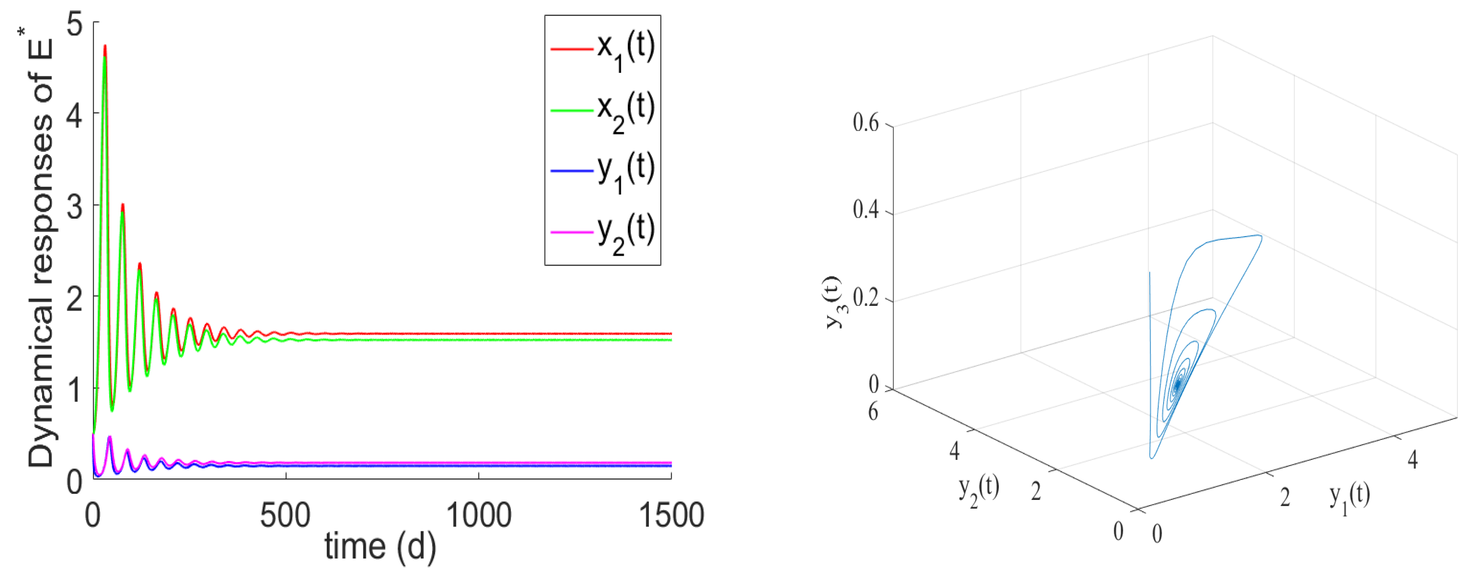
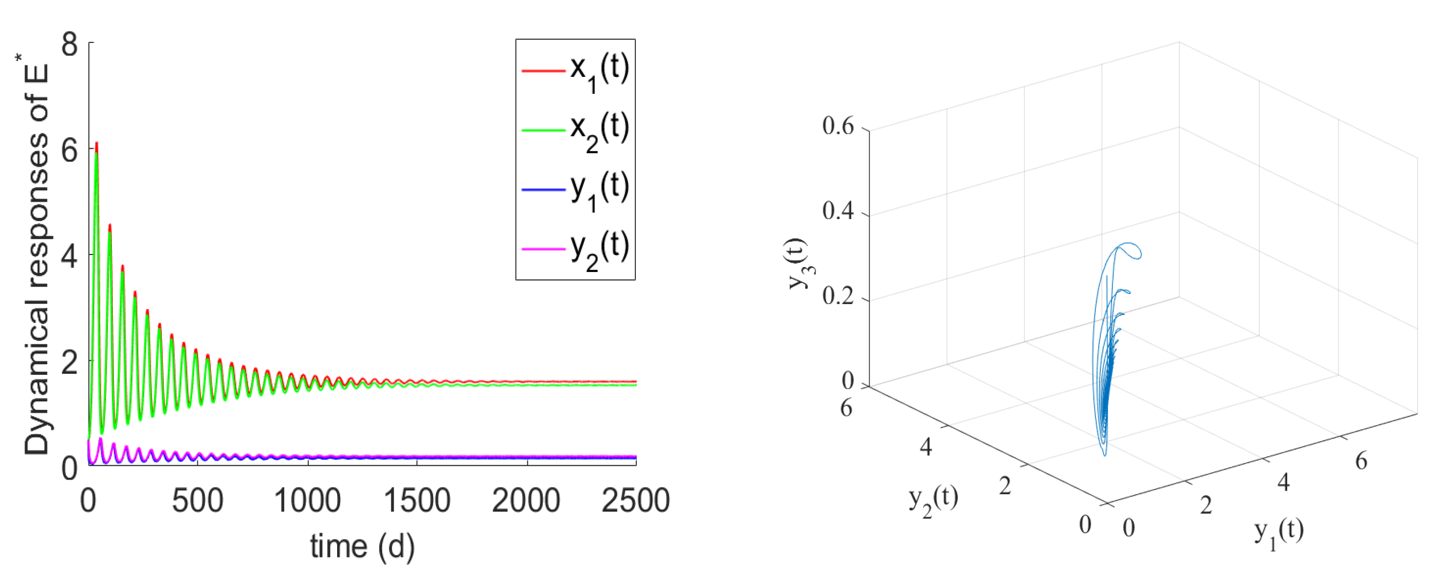
If $\left[2k_1^2{b}_2{a}_4(b_2+d_3)+k_1^2{a}_3{d}_4\right]a_{2}m+k_1^3{k}_2{b}_2<k_1^3{b}_2{d}_4(d_3+b_2),b_{1}r-d_2(b_1+d_1)>0$, the prey and predator have local stability. If $\left(H1\right),\left(H2\right)$, and $p_2^4<q_2^4$ hold, there is the positive equilibrium $E^{\ast }$ of System (2). $E^{\ast }$ is stable for $\tau <{\tau }_0$ and undergoes a Hopf bifurcation at $\tau ={\tau }_0$. From the numerical simulations Figure 1 and Figure 2, if $\tau =5$, $\tau =9$, and the other parameter values remain unchanged, we can easily to see that the unique positive equilibrium $E^{\ast }$ is local asymptotically stable. We found that the numbers of immature prey, mature prey, immature predators, and mature predators increased with the increase of maturation delay during the same period. However, over time, their numbers tended to stabilize. Moreover, as shown in Figure 3, as $\tau$ increases from 9 to 12.5, the prey and predator populations may lose their stabilities and become increasingly unstable due to the enlarged amplitudes of the oscillation intervals. Biologically, this means that a shorter incubation period of mature spaces is helpful in stabilizing the system. If the incubation period is too long, the ecosystem will be unstable. If the development time is too short, the ecological interpretation shows that there are not enough mature prey for mature predators to feed on, and the predators will be subject to cannibalism, competition, natural death, etc., and immature predators will not be able to consume enough mature prey biomass.

(3)

If $0<k_1^3{b}_2{d}_4(d_3+b_2)-\left[2k_1^2{b}_2{a}_4(b_2+d_3)+k_1^2{a}_3{d}_4\right]a_{2}m+k_1^3{k}_2{b}_2<{\overline{x}}_2$, the prey population is permanent together with the predator.

What has been and has not been proved in this article is listed as follows (see

Table 1. A Brief Summary of the Paper.

Indicating: List the sufficient conditions for the main conclusion
1	Give the sufficient conditions for the system to be uniformly bounded
	$M_1=\frac{b_1{r}^2}{4a_1(b_1+\frac{d_1}{2})\tilde{D}},$    and    $M_2=\frac{k_1{b}_1{r}^2}{4k_2{a}_2(b_1+\frac{d_1}{2})\tilde{D}},$
	$\tilde{D}=min\left\{\frac{d_1}{2},\frac{d_2(b_1+\frac{d_1}{2})}{b_1},\frac{k_1{a}_3(b_1+\frac{1}{2}{d}_1)}{b_1{k}_2},\frac{k_1{a}_4(b_1+\frac{1}{2}{d}_1)}{b_1{k}_2}\right\}.$
2	The necessary conditions for persistent existence remain to be proved
3	Give the sufficient conditions for $E_1$ to be locally asymptotically stable
	Hypothesis 4 (H4), $(d_1+b_1)(d_2+2a_2{x}_2^0)>r{b}_1$ and $k_2{b}_2>d_4(b_2+d_3)m.$
4	The necessary conditions for $E_1$ being locally asymptotically stable remain to be proved
5	Give the sufficient conditions for $E_1$ to be globally asymptotically stable
	Hypothesis 4 (H4), $(d_1+b_1)(d_2+2a_2{x}_2^0)>r{b}_1$ and $k_2{b}_2>d_4(b_2+d_3)m.$
6	The necessary conditions for $E_1$ being globally asymptotically stable remain to be proved
7	Give the sufficient conditions for $E^{\ast }$ to be locally asymptotically stable
	$p_1(p_2+q_2)>p_3+q_3,p_3(p_2+q_2)(p_3+q_3)>{(p_3+q_3)}^2+p_1^2(p_4+q_4),p_4+q_4>0$.
8	The necessary conditions for $E^{\ast }$ being globally asymptotically stable remain to be proved
9	Give the sufficient conditions for $E^{\ast }$ to be globally asymptotically stable
	$0<k_1^3{b}_2{d}_4(d_3+b_2)-\left[2k_1^2{b}_2{a}_4(b_2+d_3)+k_1^2{a}_3{d}_4\right]a_{2}m+k_1^3{k}_2{b}_2<{\overline{x}}_2.$
10	The necessary conditions for $E^{\ast }$ being globally asymptotically stable remain to be proved

), which will give the reader a clearer idea of what issues this article addresses.

6. Conclusions

In this manuscript, we study the modified stage-structured predator–prey system with Holling III functional response and cannibalism. By analyzing corresponding characteristic equations, sufficient conditions for the local asymptotic stability of the positive equilibrium are derived and the existence of the Hopf bifurcation of each feasible equilibrium is addressed. By using the persistence theory for infinite-dimensional systems and the comparison principle, the sufficient conditions for the uniform persistence of the system are obtained. According to the characteristics of the model, by constructing the Liapunov functional, for each equilibrium point of the system we prove global stability separately. Using Theorems 1 and 2, we set the values of each parameter in the system and obtain the system’s branching critical value ${\tau }_0$. When the time delay $\tau$ goes from 5 to 9, the positive equilibrium $E^{\ast }(x_1^{\ast },x_2^{\ast },y_1^{\ast },y_2^{\ast })$ remains stable permanently. When the time delay $\tau$ goes from 9 to 12.50 and passes through the critical values ${\tau }_0=12.1391$, the positive equilibrium $E^{\ast }$ loses its stability and a Hopf bifurcation occurs. According to Theorems 3 and 4, under a set of parameter values, we see that the predator is extinct but the prey is permanent, while under another set of parameter values both of them are permanent. Numerical analysis verifies the correctness of the theoretical analysis. The model is close to the actual situation in nature, and the obtained theorems can be used to judge the conditions of continuous survival and the extinction of populations at different stages. These conclusions have a certain application value in ecological balance control.

References

- Maitra, S. Dynamical behaviour of a delayed three species predator–prey model with cooperation among the prey species. Nonlinear Dyn. 2018, 92, 627–643. [Google Scholar]
- Zha, L.; Cui, J.A.; Zhou, X. Ratio-dependent predator-prey model with stage structure and time delay. Int. J. Biomath. 2012, 5, 15–37. [Google Scholar] [CrossRef]
- Biswas, S.; Saifuddin, M.; Sasmal, S.K.; Samanta, S.; Chattopadhyay, J. A delayed prey–predator system with prey subject to the strong Allee effect and disease. Nonlinear Dyn. 2016, 84, 1569–1594. [Google Scholar] [CrossRef]
- Yang, R.; Wei, J. Stability and bifurcation analysis of a diffusive prey–predator system in Holling type III with a prey refuge. Nonlinear Dyn. 2015, 79, 631–646. [Google Scholar] [CrossRef]
- Meng, X.Y.; Wang, J.G. Dynamical analysis of a delayed diffusive predator–prey model with schooling behaviour and Allee effect. J. Biol. Dyn. 2020, 84, 826–848. [Google Scholar] [CrossRef]
- Dubey, B.; Agarwal, S.; Kumar, A. Optimal harvesting policy of a prey–predator model with Crowley–Martin-type functional response and stage structure in the predator. Nonlinear Anal. Model. Control 2018, 23, 493–514. [Google Scholar] [CrossRef]
- Zhang, X.; Liu, Z. Hopf bifurcation analysis in a predator-prey model with predator-age structure and predator-prey reaction time delay. Appl. Math. Model. 2021, 91, 530–548. [Google Scholar] [CrossRef]
- Yuan, Y. Stability and Hopf bifurcation in delayed prey–predator system with ratio dependent. Appl. Mech. Mater. 2014, 687–691, 655–660. [Google Scholar] [CrossRef]
- Gao, S.; Chen, L. Permanence and global stability for single-species model with three life stages and time delay. Acta Math. Sci. 2006, 26, 527–533. [Google Scholar]
- Liang, Z.; Li, B.; Jin, S. Stability and travelling waves for a time-delayed population system with stage structure. Nonlinear Anal. Real World Appl. 2012, 13, 1429–1440. [Google Scholar]
- Han, L. Data processing for cynamic consequences of prey refuge in a prey–predator system with stage structure and time delay. Adv. Mater. Res. 2014, 978, 88–93. [Google Scholar] [CrossRef]
- Xia, Y.H.; Romanovski, V.G. Bifurcation analysis of a population dynamics in a critical state. Bull. Malays. Math. Soc. Ser. 2015, 38, 499–527. [Google Scholar] [CrossRef]
- Bhattacharyya, J.; Piiroinen, P.T.; Banerjee, S. Dynamics of a Filippov prey–predator system with stage-specific intermittent harvesting. Nonlinear Dynam. 2021, 105, 1019–1043. [Google Scholar] [CrossRef]
- Morozov, A.Y.; Banerjee, M.; Petrovskii, S.V. Long-term transients and complex dynamics of a stage-structured population with time delay and the Allee effect. J. Theor. Biol. 2016, 396, 116–124. [Google Scholar] [CrossRef] [PubMed]
- Zhang, H.T.; Li, L. Traveling wave fronts of a single species model with cannibalism and nonlocal effect. Chaos Solitons Fractals 2018, 108, 148–153. [Google Scholar] [CrossRef]
- Xu, D. Global dynamics and Hopf bifurcation of a structured population model. Nonlinear Anal.-Real. 2005, 6, 461–476. [Google Scholar] [CrossRef]
- Yu, X.; Zhu, Z.; Chen, F. Dynamic behaviors of a single species stage structure model with Michaelis-Menten-type juvenile population harvesting. Mathematics 2020, 8, 1281. [Google Scholar] [CrossRef]
- Rayungsari, M.; Suryanto, A.; Kusumawinahyu, W.M.; Darti, I. Dynamical analysis of a predator-prey model incorporating predator cannibalism and refuge. Axioms 2022, 11, 116. [Google Scholar] [CrossRef]
- Wang, L.; Xu, R. Global dynamics of a prey–predator model with stage structure and delayed predator response. Discret. Dyn. Nat. Soc. 2013, 2013, 724325. [Google Scholar] [CrossRef]
- Wang, L.; Feng, G. Global stability and Hopf bifurcation of a prey–predator model with time delay and stage structure. Chin. J. Eng. Math. 2014, 2014, 431671. [Google Scholar] [CrossRef]
- Wang, L.; Feng, G. Stability and Hopf bifurcation for a ratio-dependent prey–predator system with stage structure and time delay. Adv. Differ. Equ. 2015, 2015, 255. [Google Scholar] [CrossRef][Green Version]
- Wang, L.; Xu, R.; Feng, G. Global dynamics of a delayed predator–prey model with stage structure and holling type II functional response. J. Appl. Math. Comput. 2015, 47, 73–89. [Google Scholar] [CrossRef]
- Wang, L.; Feng, G. Global dynamics of a delayed prey–predator model with stage structure for the predator and the prey. Math. Methods Appl. Sci. 2015, 38, 3937–3949. [Google Scholar] [CrossRef]
- Zhu, H.; Gao, D. Stability and Hopf bifurcation in a time-delayed predator-prey system with stage structures for both predator and prey. Chin. J. Eng. Math. 2020, 36, 693–707. [Google Scholar]
- Wei, Y.; Zhu, H. Stability and Hopf bifurcation in a predator-prey system with Holling-III functional response and stage structure. J. Nat. Sci. Heilongjiang Univ. 2019, 36, 39–46. [Google Scholar]
- Sajjadi, S.S.; Baleanu, D.; Jajarmi, A.; Pirouz, H.M. A new adaptive synchronization and hyperchaos control of a biological snap oscillator. Chaos Solitons Fractals 2020, 138, 109919. [Google Scholar] [CrossRef]
- Srivastava, H.; Khader, M. Numerical simulation for the treatment of nonlinear predator-prey equations by using the finite element optimization method. Fractal Fract. 2021, 5, 56. [Google Scholar] [CrossRef]
- Djilali, S.; Mezouaghi, A.; Belhamiti, O. Bifurcation analysis of a diffusive predator-prey model with schooling behaviour and cannibalism in prey. Appl. Math. Inf. Sci. 2021, 11, 209. [Google Scholar] [CrossRef]
- Nishikawa, M.; Ferrero, N.; Cheves, S.; Lopez, R.; Kawamura, S.; Fedigan, L.M.; Melin, A.D.; Jack, K.M. Infant cannibalism in wild white-faced capuchin monkeys. Ecol. Evol. 2020, 10, 12679–12684. [Google Scholar] [CrossRef]
- Kang, Y.; Rodriguez-Rodriguez, M.; Evilsizor, S. Ecological and evolutionary dynamics of two-stage models of social insects with egg cannibalism. J. Math. Anal. Appl. 2015, 430, 324–353. [Google Scholar] [CrossRef]
- Zhang, F.; Chen, Y.; Li, J. Dynamical analysis of a stage-structured predator-prey model with cannibalism. Math. Biosci. 2019, 307, 33–41. [Google Scholar] [CrossRef] [PubMed]
- Deng, H.; Chen, F.; Zhu, Z.; Li, Z. Dynamic behaviors of Lotka-Volterra predator-prey model incorporating predator cannibalism. Adv. Differ. Equ. 2019, 2019, 359. [Google Scholar] [CrossRef]
- Ma, Z.E.; Zhou, Y.C. Qualitative and Stable Methods for Ordinary Differential Equations; Science Press: Beijing, China, 2001. [Google Scholar]
- Chen, M.; Yang, X.; Fu, S. Global behavior of solutions in a prey–predator cross-diffusion model with cannibalism. Complexity 2020, 2020, 1265798. [Google Scholar] [CrossRef]
- Hale, J.K.; Waltman, P. Persistence in infinite-dimensional systems. J. Math. Anal. 1989, 20, 388–395. [Google Scholar] [CrossRef]