ISI-Equienergetic Graphs

Abstract

The ISI-energy ${\epsilon }_{isi}\left(G\right)$ of a graph $G=(V,E)$ is the sum of the absolute values of the eigenvalues of the ISI-matrix $\mathcal{C}\left(G\right)={\left[c_{ij}\right]}_{n\times n}$ in which $c_{ij}=\frac{d\left(v_i\right)d\left(v_j\right)}{d\left(v_i\right)+d\left(v_j\right)}$ if $v_i{v}_j\in E\left(G\right)$ and $c_{ij}=0$ otherwise. $d\left(v_i\right)$ denotes the degree of vertex $v_i\in V$. As a class of graph energy, ISI-energy can be utilized to ascertain the general energy of conjugated carbon molecules. Two non-isomorphic graphs of the same order are said to be ISI-equienergetic if their ISI-energies are equal. In this paper, we construct pairs of connected, ISI-noncospectral, ISI-equienergetic graphs of order n for all $n\ge 9$. In addition, for n-vertex $r(r\ge 3)$-regular graph G, and for each $k\ge 2$, we obtain ${\epsilon }_{isi}(\overline{L^k(G)})$, depending only on n and r. This result enables a systematic construction of pairs of ISI-noncospectral graphs of the same order, having equal ISI-energies.

1. Introduction

A graph $G=\left(V\right(G),E(G\left)\right)$ is a mathematical structure composed of two finite sets $V\left(G\right)$ and $E\left(G\right)$. The elements of $V\left(G\right)$ are called vertices (or nodes), and the elements of $E\left(G\right)$ are called edges. For $v_i\in V\left(G\right)$, $N\left(v_i\right)$ denotes the set of its neighbors in G, and the degree of $v_i$ is $d\left(v_i\right)=\left|N\left(v_i\right)\right|$. An n-vertex graph denotes the graph of order n. A graph with only r-vertices is called an r-regular graph. Throughout the article, only finite simple undirected graphs are considered. We use Bondy and Murty [1] for terminology and notations not defined here.

The ISI index is an interesting topological index which can distinctively forecast the superficial area for isomers of octanes [2]. The ISI index of graph G is defined as

$$ISI\left(G\right)=\sum _{v_i{v}_j\in E\left(G\right)}\frac{d\left(v_i\right)d\left(v_j\right)}{d\left(v_i\right)+d\left(v_j\right)}.$$

The ISI-matrix $\mathbf{C}=\mathbf{C}\left(G\right)$ of the graph G is defined as the matrix with entries [3,4,5]:

$$c_{ij}:=\left\{\begin{array}{cc}\frac{d\left(v_i\right)d\left(v_j\right)}{d\left(v_i\right)+d\left(v_j\right)},\hfill & if{v}_i{v}_j\in E\left(G\right)\hfill \\ 0,\hfill & otherwise.\hfill \end{array}\right.$$

Note that $\mathbf{C}$ is a modification of the classical adjacency matrix.

The characteristic polynomial of $\mathbf{C}\left(G\right)$ is called the ISI-characteristic polynomial of n-vertex graph G, defined as $\Phi (\mathbf{C}\left(G\right),\mu )=det(\mu {\mathbf{I}}_n-\mathbf{C}\left(G\right))$, where ${\mathbf{I}}_n$ is the unit matrix of order n. The eigenvalues of the ISI-matrix $\mathbf{C}\left(G\right)$, denoted by ${\mu }_1\ge {\mu }_2\ge \dots \ge {\mu }_n$, are said to be the ISI-eigenvalues of G. In [3], we proved that the sum of the ISI-eigenvalues of G is zero.

Let $\mathbf{A}$ denote the adjacency matrix of a graph G of order n. Because $\mathbf{A}$ and $\mathbf{C}$ are real symmetric matrices, their eigenvalues are real numbers. Denote by ${\lambda }_1\ge {\lambda }_2\ge \dots \ge {\lambda }_n$ the ordered eigenvalues of $\mathbf{A}$. The characteristic polynomial of the matrix $\mathbf{A}$ is the characteristic polynomial of G, denoted by $\Phi (G,\lambda )=det(\lambda I-\mathbf{A})$. If ${\lambda }_1,{\lambda }_2,\dots ,{\lambda }_k$ are the distinct eigenvalues of G with respective multiplicities $m_1,m_2,\dots ,m_k$, then the spectrum of G is denoted by

$$Spec\left(G\right)=\left(\begin{array}{cc}& {\lambda }_1{\lambda }_2\dots {\lambda }_k\hfill \\ & m_1{m}_2\dots m_k\hfill \end{array}\right).$$

Topological molecular descriptors based on eigenvalues are widely used in chemical research [6,7]. It is possible that the graph energy [8,9,10] is the most studied descriptor of this kind, which is mainly used to describe the stability of conjugated molecules. The energy [8] of an n-vertex graph G is defined as

$$\epsilon =\epsilon \left(G\right)=\sum _{i=1}^n\left|{\lambda }_i\right|.$$

(1)

Generalizing the energy concept to the ISI-matrix, the ISI-energy [4,11] is defined as below

$${\epsilon }_{isi}={\epsilon }_{isi}\left(G\right)=\sum _{i=1}^n\left|{\mu }_i\right|.$$

(2)

It is worth noting that $\epsilon \left(G\right)$ and ${\epsilon }_{isi}\left(G\right)$ of graphs are closely linked, and we can determine $\epsilon \left(G\right)$ by means of ${\epsilon }_{isi}\left(G\right)$. Consequently, the ${\epsilon }_{isi}\left(G\right)$ study is not only of theoretical meaning but also of realistic value.

When two graphs $G_1$ and $G_2$ have different structures, it is taken for granted that ${\epsilon }_{isi}\left(G_1\right)\ne {\epsilon }_{isi}\left(G_2\right)$. Nevertheless, it is not always true by observation. That is, two structurally different graphs can have equal ISI-energy. For example, take into account the cycles $C_3$ and $C_4$. The ISI-eigenvalues of $C_3$ and $C_4$ are $1,-\frac{1}{2},\frac{1}{2}$ and $1,0,0,1$, respectively. Hence, ${\epsilon }_{isi}\left(C_3\right)={\epsilon }_{isi}\left(C_4\right)$. This observation results in the conception of ISI-equienergetic graphs.

Two non-isomorphic graphs are said to be ISI-cospectral if they have the same ISI-eigenvalues. The graphs $G_1$ and $G_2$ are said to be ISI-equienergetic if ${\epsilon }_{isi}\left(G_1\right)={\epsilon }_{isi}\left(G_2\right)$. Apparently, two ISI-cospectral graphs must be ISI-equienergetic, but the converse is not always true in common cases. Thus, we are interested in the construction of ISI-equienergetic pairs of graphs which are ISI-noncospectral.

If we do not restrict two graphs to have the same number of vertices, it is extremely simple to construct ISI-noncospectral, ISI-equienergetic graphs. Let G be any graph with ISI-spectrum ${\mu }_1,{\mu }_2,\dots ,{\mu }_n$, and let $G_0$ be the graph obtained by adding arbitrarily $t(t\ge 1)$ number of isolated vertices to G, then the spectrum of $G_0$ consists of the numbers ${\mu }_1,{\mu }_2,\dots ,{\mu }_n$, ${\mu }_{n+1}=0,{\mu }_{n+2}=0,\dots ,{\mu }_{n+t}=0$. Thus, G and $G_0$ are not ISI-cospectral but ${\epsilon }_{isi}\left(G\right)={\epsilon }_{isi}\left(G_0\right)$.

If we also require this kind of graph to have the same order and equal number of edges (which is of great value in chemical applications), the problem becomes not so easy. As we know, up to now, there exists no systematic approach for constructing pairs (or larger families) of ISI-equienergetic graphs. Therefore, it is interesting to obtain ISI-noncospectral graphs on the same number of vertices having equal ISI-energy. Our results can quickly obtain the ISI-energy of the ISI-noncospectral, ISI-equienergetic graphs, which can greatly reduce the workload of calculating the ISI-energy of graphs.

This paper is organized as follows. We first obtain the characteristic polynomial of the ISI-matrix of the join of two regular graphs and thereby construct pairs of ISI-noncospectral, ISI-equienergetic graphs on n vertices for all $n\ge 9$. Furthermore, for n-vertex $r(r\ge 3)$-regular graph G, and for each $k\ge 2$, we obtain ${\epsilon }_{isi}(\overline{L^k(G)})$, depending only on n and r. This result enables a systematic construction of pairs of ISI-noncospectral graphs of the same order, having equal ISI-energies.

2. ISI-Equienergetic Graphs

In this section, we pay our attention to constructions of ISI-noncospectral, ISI-equienergetic graphs.

Let G and H be two graphs. The join $G+H$ of G and H is the graph with vertex set $V(G+H)=V\left(G\right)\cup V\left(H\right)$, and the edge set $E(G+H)$ is obtained by joining each of the vertices of $V\left(G\right)$ to all the vertices of $V\left(H\right)$.

We denote by ${\mathbf{J}}_{n_1\times n_2}$ the $n_1\times n_2$ matrix having all its entries as 1. It can be noted that if G is a k-regular graph, then $\mathbf{C}\left(G\right)=\frac{k}{2}\mathbf{A}\left(G\right)$.

In the following theorem, we give the ISI-characteristic polynomial of $G+H$ when both G and H are regular graphs.

Theorem 1.

Let $G_i$ be an $n_i$-vertex $r_i$-regular graph for $i=1,2$. Then, the ISI-characteristic polynomial of $G=G_1+G_2$ is

$$\Phi (\mathbf{C}\left(G\right),\mu )=\frac{(\mu -X)(\mu -Y)-n_1{n}_2{a}^2}{(\mu -X)(\mu -Y)}\Phi ({\mathbf{C}}^{\prime }\left(G_1\right),\mu )\Phi ({\mathbf{C}}^{\prime }\left(G_2\right),\mu ),$$

(3)

where $X=\frac{(r_1+n_2)r_1}{2}$, $Y=\frac{(r_2+n_1)r_2}{2}$, $a=\frac{(n_1+r_2)(n_2+r_1)}{n_1+n_2+r_2+r_1}$, ${\mathbf{C}}^{\prime }\left(G_1\right)=\frac{r_1+n_2}{r_1}\mathbf{C}\left(G_1\right)$, ${\mathbf{C}}^{\prime }\left(G_2\right)=\frac{r_2+n_1}{r_2}\mathbf{C}\left(G_2\right)$.

Proof. 

As $G_i$ is an $n_i$-vertex $r_i$-regular graph for $i=1,2$, we have

$$\mathbf{C}(G_1+G_2)=\left(\begin{array}{cc}{\mathbf{C}}^{\prime }\left(G_1\right)& a{\mathbf{J}}_{n_1\times n_2}\\ a{\mathbf{J}}_{n_2\times n_1}& {\mathbf{C}}^{\prime }\left(G_2\right)\end{array}\right),$$

(4)

where $a=\frac{(n_1+r_2)(n_2+r_1)}{n_1+n_2+r_2+r_1}$.

And we obtain

$$\Phi (\mathbf{C}\left(G\right),\mu )=det(\mu {\mathbf{I}}_n-\mathbf{C}\left(G\right))=\left|\begin{array}{cc}\mu {\mathbf{I}}_{n_1}-{\mathbf{C}}^{\prime }\left(G_1\right)& -a{\mathbf{J}}_{n_1\times n_2}\\ -a{\mathbf{J}}_{n_2\times n_1}& \mu {\mathbf{I}}_{n_2}-{\mathbf{C}}^{\prime }\left(G_2\right)\end{array}\right|.$$

(5)

Let

$$c_{ij}:=\left\{\begin{array}{cc}\frac{d\left(v_i\right)d\left(v_j\right)}{d\left(v_i\right)+d\left(v_j\right)},\hfill & if{v}_i{v}_j\in E\left(G_1\right)\hfill \\ 0,\hfill & otherwise.\hfill \end{array}\right.$$

and

$$c_{ij}^{\prime }:=\left\{\begin{array}{cc}\frac{d\left(u_i\right)d\left(u_j\right)}{d\left(u_i\right)+d\left(u_j\right)},\hfill & if{u}_i{u}_j\in E\left(G_2\right)\hfill \\ 0,\hfill & otherwise.\hfill \end{array}\right.$$

Determinant (5) can be written as

$$\left|\begin{array}{cccccccc}\mu & -c_{12}& \dots & -c_{1n_1}& -a& -a& \dots & -a\\ -c_{21}& \mu & \dots & -c_{1n_1}& -a& -a& \cdots & -a\\ ⋮& ⋮& ⋮& ⋮& ⋮& ⋮& ⋮& ⋮\\ -c_{n_{1}1}& -c_{n_{1}2}& \dots & \mu & -a& -a& \cdots & -a\\ -a& -a& \dots & -a& \mu & -c_{12}^{\prime }& \cdots & -c_{1n_2}^{\prime }\\ -a& -a& \dots & -a& -c_{21}^{\prime }& \mu & \cdots & -c_{2n_2}^{\prime }\\ ⋮& ⋮& ⋮& ⋮& ⋮& ⋮& ⋮& ⋮\\ -a& -a& \dots & -a& -c_{n_{2}1}^{\prime }& -c_{n_{2}2}^{\prime }& \cdots & \mu \end{array}\right|$$

(6)

It is obvious that

$$\sum _{j=1}^{n_1}{c}_{ij}=\frac{(r_1+n_2)r_1}{2}=X$$

(7)

for $i=1,2,\dots ,n_1$, and

$$\sum _{j=1}^{n_2}{c}_{ij}^{\prime }=\frac{(r_2+n_1)r_2}{2}=Y$$

(8)

for $i=1,2,\dots ,n_2$.

By subtracting the row $(n_1+1)$ from the rows $(n_1+2),(n_1+3)$,…, $(n_1+n_2)$ of determinant (6), we obtain determinant (9).

$$\left|\begin{array}{cccccccc}\mu & -c_{12}& \dots & -c_{1n_1}& -a& -a& \dots & -a\\ -c_{21}& \mu & \dots & -c_{1n_1}& -a& -a& \cdots & -a\\ ⋮& ⋮& ⋮& ⋮& ⋮& ⋮& ⋮& ⋮\\ -c_{n_{1}1}& -c_{n_{1}2}& \dots & \mu & -a& -a& \cdots & -a\\ -a& -a& \dots & -a& \mu & -c_{12}^{\prime }& \cdots & -c_{1n_2}^{\prime }\\ 0& 0& \dots & 0& -\mu -c_{21}^{\prime }& \mu +c_{12}^{\prime }& \cdots & -c_{2n_2}^{\prime }+c_{1n_2}^{\prime }\\ ⋮& ⋮& ⋮& ⋮& ⋮& ⋮& ⋮& ⋮\\ 0& 0& \dots & 0& -\mu -c_{n_{2}1}^{\prime }& -c_{n_{2}2}^{\prime }+c_{12}^{\prime }& \cdots & \mu +c_{1n_2}^{\prime }\end{array}\right|$$

(9)

Add the columns $(n_1+2),(n_1+3)$,…, $(n_1+n_2)$ to the column $(n_1+1)$ of determinant (9), we obtain determinant (10).

$$\left|\begin{array}{cccccccc}\mu & -c_{12}& \dots & -c_{1n_1}& -an& -a& \dots & -a\\ -c_{21}& \mu & \dots & -c_{1n_1}& -an& -a& \cdots & -a\\ ⋮& ⋮& ⋮& ⋮& ⋮& ⋮& ⋮& ⋮\\ -c_{n_{1}1}& -c_{n_{1}2}& \dots & \mu & -an& -a& \cdots & -a\\ -a& -a& \dots & -a& \mu -Y& -c_{12}^{\prime }& \cdots & -c_{1n_2}^{\prime }\\ 0& 0& \dots & 0& 0& \mu +c_{12}^{\prime }& \cdots & -c_{2n_2}^{\prime }+c_{1n_2}^{\prime }\\ ⋮& ⋮& ⋮& ⋮& ⋮& ⋮& ⋮& ⋮\\ 0& 0& \dots & 0& 0& -c_{n_{2}2}^{\prime }+c_{12}^{\prime }& \cdots & \mu +c_{1n_2}^{\prime }\end{array}\right|$$

(10)

For convenience, we let

$$\left|\mathbf{B}\right|=\left|\begin{array}{cccc}\mu +c_{12}^{\prime }& -c_{23}^{\prime }+c_{13}^{\prime }& \cdots & -c_{2n_2}^{\prime }+c_{1n_2}^{\prime }\\ -c_{32}^{\prime }+c_{12}^{\prime }& \mu +c_{13}^{\prime }& \cdots & -c_{3n_2}^{\prime }+c_{1n_2}^{\prime }\\ ⋮& ⋮& ⋮& ⋮\\ -c_{n_{2}2}^{\prime }+c_{12}^{\prime }& -c_{n_{2}3}^{\prime }+c_{13}^{\prime }& \cdots & \mu +c_{1n_2}^{\prime }\end{array}\right|$$

(11)

Subtract the first row from the rows $2,3,\dots ,n_1$ of determinant (10), and we obtain determinant (12).

$$\left|\begin{array}{cccccccc}\mu & -c_{12}& \dots & -c_{1n_1}& -an& -a& \dots & -a\\ -c_{21}-\mu & \mu +c_{12}& \dots & 0& 0& 0& \cdots & 0\\ ⋮& ⋮& ⋮& ⋮& ⋮& ⋮& ⋮& ⋮\\ -c_{n_{1}1}-\mu & -c_{n_{1}2}+c_{12}& \dots & \mu +c_{1n_1}& 0& 0& \cdots & 0\\ -a& -a& \dots & -a& \mu -Y& -c_{12}^{\prime }& \cdots & -c_{1n_2}^{\prime }\\ 0& 0& \dots & 0& 0& \mu +c_{12}^{\prime }& \cdots & -c_{2n_2}^{\prime }+c_{1n_2}^{\prime }\\ ⋮& ⋮& ⋮& ⋮& ⋮& ⋮& ⋮& ⋮\\ 0& 0& \dots & 0& 0& -c_{n_{2}2}^{\prime }+c_{12}^{\prime }& \cdots & \mu +c_{1n_2}^{\prime }\end{array}\right|$$

(12)

Add the columns $2,3,\dots ,n_1$ to the first column of determinant (12), and we arrive at determinant (13).

$$\left|\begin{array}{ccccc}\mu -X& -c_{12}& \dots & -c_{1n_1}& -a{n}_2\\ 0& \mu +c_{12}& \dots & -c_{1n_1}+c_{1n_1}& 0\\ ⋮& ⋮& ⋮& ⋮& ⋮\\ 0& -c_{n_{1}2}+c_{12}& \dots & \mu +c_{1n_1}& 0\\ -a{n}_1& -a& \dots & -a& \mu -Y\end{array}\right|\left|\mathbf{B}\right|$$

(13)

Expand determinant (13) along the first column to obtain (14):

$$det(\mu {\mathbf{I}}_n-\mathbf{C}\left(G\right))=(\mu -X)|{\mathbf{D}}_1{|-(-1)}^{n_1}a{n}_1|{\mathbf{D}}_2\left|\right)\left|\mathbf{B}\right|$$

(14)

where

$$|{\mathbf{D}}_1|=\left|\begin{array}{ccccc}\mu +c_{12}& -c_{23}+c_{13}& \dots & -c_{1n_1}+c_{1n_1}& 0\\ -c_{32}+c_{12}& \mu +c_{13}& \dots & -c_{3n_1}+c_{1n_1}& 0\\ ⋮& ⋮& ⋮& ⋮& ⋮\\ -c_{n_{1}2}+c_{12}& -c_{n_{1}3}+c_{13}& \dots & \mu +c_{1n_1}& 0\\ -a& -a& \dots & -a& \mu -Y\end{array}\right|$$

$$|{\mathbf{D}}_2|=\left|\begin{array}{ccccc}-c_{12}& -c_{13}& \dots & -c_{1n_1}& -a{n}_2\\ \mu +c_{12}& -c_{23}+c_{13}& \dots & -c_{2n_1}+c_{1n_1}& 0\\ -c_{32}+c_{12}& \mu +c_{13}& \dots & -c_{3n_1}+c_{1n_1}& 0\\ ⋮& ⋮& ⋮& ⋮& ⋮\\ -c_{n_{1}2}+c_{12}& -c_{n_{1}3}+c_{13}& \dots & \mu +c_{1n_1}& 0\end{array}\right|$$

Let

$$\left|\mathbf{A}\right|=\left|\begin{array}{cccc}\mu +c_{12}& -c_{23}+c_{13}& \dots & -c_{2n_1}+c_{1n_1}\\ -c_{32}+c_{12}& \mu +c_{13}& \dots & -c_{3n_1}+c_{1n_1}\\ ⋮& ⋮& ⋮\\ -c_{n_{1}2}+c_{12}& -c_{n_{1}3}+c_{13}& \dots & \mu +c_{1n_1}\end{array}\right|$$

Expression (14) can be written as

$$\begin{array}{ccc}\hfill det(\mu {\mathbf{I}}_n-\mathbf{C}\left(G\right))& =& \left((\mu -X)(\mu -Y)\left|\mathbf{A}\right|-{(-1)}^{n_1}a{n}_1{(-1)}^{n_1+1}(-n_{2}a)\left|\mathbf{A}\right|\right)\left|\mathbf{B}\right|\hfill \\ \hfill & =& \left((\mu -X)(\mu -Y)-n_1{n}_2{a}^2)\right)\left|\mathbf{A}\right|\left|\mathbf{B}\right|\hfill \end{array}$$

(15)

On the other hand, the determinant $\left|\mathbf{A}\right|$ can be written as

$$\left|\mathbf{A}\right|=\frac{1}{\mu -X}\left|\begin{array}{ccccc}\mu -X& -c_{12}& -c_{13}& \dots & -c_{1n_1}\\ 0& \mu +c_{12}& -c_{23}+c_{13}& \dots & -c_{2n_1}+c_{1n_1}\\ 0& -c_{32}+c_{12}& \mu +c_{13}& \dots & -c_{3n_1}+c_{1n_1}\\ ⋮& ⋮& ⋮& ⋮\\ 0& -c_{n_{1}2}+c_{12}& -c_{n_{1}3}+c_{13}& \dots & \mu +c_{1n_1}\end{array}\right|$$

Let

$$\left|\mathbf{H}\right|=\left|\begin{array}{ccccc}\mu -X& -c_{12}& -c_{13}& \dots & -c_{1n_1}\\ 0& \mu +c_{12}& -c_{23}+c_{13}& \dots & -c_{2n_1}+c_{1n_1}\\ 0& -c_{32}+c_{12}& \mu +c_{13}& \dots & -c_{3n_1}+c_{1n_1}\\ ⋮& ⋮& ⋮& ⋮\\ 0& -c_{n_{1}2}+c_{12}& -c_{n_{1}3}+c_{13}& \dots & \mu +c_{1n_1}\end{array}\right|$$

(16)

From equation (7), the sum of the i-th row in (16) is $\mu +c_{i1}$ for $i=2,3,\dots ,n_1$. By subtracting columns $2,3,\dots ,n_1$ of determinant (16) from the first column, we obtain determinant (17).

$$\left|\mathbf{H}\right|=\left|\begin{array}{ccccc}\mu & -c_{12}& -c_{13}& \dots & -c_{1n_1}\\ -\mu -c_{21}& \mu +c_{12}& -c_{23}+c_{13}& \dots & -c_{2n_1}+c_{1n_1}\\ -\mu -c_{31}& -c_{32}+c_{12}& \mu +c_{13}& \dots & -c_{3n_1}+c_{1n_1}\\ ⋮& ⋮& ⋮& ⋮\\ -\mu -c_{n_{1}1}& -c_{n_{1}2}+c_{12}& -c_{n_{1}3}+c_{13}& \dots & \mu +c_{1n_1}\end{array}\right|$$

(17)

Add the first row of $\left|\mathbf{H}\right|$ to the rows $2,3,\dots ,n_1$, and we obtain determinant (18).

$$\left|\mathbf{H}\right|=\left|\begin{array}{ccccc}\mu & -c_{12}& -c_{13}& \dots & -c_{1n_1}\\ -c_{21}& \mu & -c_{23}& \dots & -c_{2n_1}\\ -c_{31}& -c_{32}& \mu & \dots & -c_{3n_1}\\ ⋮& ⋮& ⋮& ⋮\\ -c_{n_{1}1}& -c_{n_{1}2}& -c_{n_{1}3}& \dots & \mu \end{array}\right|$$

(18)

Then, we have

$$\left|\mathbf{A}\right|=\frac{1}{\mu -X}\left|\mathbf{H}\right|=\frac{1}{\mu -X}\Phi ({\mathbf{C}}^{\prime }\left(G_1\right),\mu )$$

(19)

In a similar way, we can obtain

$$\left|\mathbf{B}\right|=\frac{1}{\mu -Y}\left|\mathbf{H}\right|=\frac{1}{\mu -Y}\Phi ({\mathbf{C}}^{\prime }\left(G_2\right),\mu )$$

(20)

Substituting (19) and (20) back into (15) gives the result. □

Lemma 1

([12]). Let λ be an eigenvalue of square matrix $\mathbf{A}$, and $\mathbf{x}$ is its eigenvector. For any real number $k\ne 0$, $k\lambda$ be an eigenvalue of square matrix $k\mathbf{A}$ corresponding to the eigenvector $\mathbf{x}$.

Theorem 2.

Let $G_i$ be an $r_i$-regular graph of order $n_i$ for $i=1,2$. Then, the ISI-energy of $G=G_1+G_2$ is

$${\epsilon }_{isi}\left(G\right)=\frac{r_1+n_2}{r_1}{\epsilon }_{isi}\left(G_1\right)+\frac{r_2+n_1}{r_2}{\epsilon }_{isi}\left(G_2\right)-\left(\frac{(n_2+r_1)r_1}{2}+\frac{(n_1+r_2)r_2}{2}\right)$$

$$+\frac{1}{2}\sqrt{{((n_2+r_1)r_1-(n_1+r_2)r_2)}^2+16n_1{n}_2{\left(\frac{(n_1+r_2)(n_2+r_1)}{n_1+n_2+r_2+r_1}\right)}^2}$$

Proof. 

By Theorem 1, we have

$$\Phi (\mathcal{C}\left(G\right),\mu )=\frac{(\mu -X)(\mu -Y)-n_1{n}_2{a}^2}{(\mu -X)(\mu -Y)}\Phi ({\mathcal{C}}^{\prime }\left(G_1\right),\mu )\Phi ({\mathcal{C}}^{\prime }\left(G_2\right),\mu )$$

i.e.,

$$(\mu -X)(\mu -Y)\Phi (\mathcal{C}\left(G\right),\mu )=[(\mu -X)(\mu -Y)-n_1{n}_2{a}^2]\Phi ({\mathcal{C}}^{\prime }\left(G_1\right),\mu )\Phi ({\mathcal{C}}^{\prime }\left(G_2\right),\mu )$$

Let

$$P_1\left(\mu \right)=(\mu -X)(\mu -Y)\Phi (\mathcal{C}\left(G\right),\mu )$$

and

$$P_2\left(\mu \right)=[(\mu -X)(\mu -Y)-n_1{n}_2{a}^2]\Phi ({\mathcal{C}}^{\prime }\left(G_1\right),\mu )\Phi ({\mathcal{C}}^{\prime }\left(G_2\right),\mu ).$$

It is obvious that the roots of $P_1\left(\mu \right)=0$ are $X,Y$ and the ISI-eigenvalues of $G_1+G_2$. Hence, the sum of the absolute values of the roots of $P_1\left(\mu \right)=0$ is $X+Y+{\epsilon }_{isi}(G_1+G_2)$.

The roots of $P_2\left(\mu \right)=0$ are ISI-eigenvalues of ${\mathcal{C}}^{\prime }\left(G_1\right)$ and ${\mathcal{C}}^{\prime }\left(G_2\right)$ and

$$\frac{X+Y}{2}\pm \frac{1}{2}\sqrt{{(X+Y)}^2-4XY+4n_1{n}_2{a}^2}.$$

It is easy to see that ${\mathcal{C}}^{\prime }\left(G_1\right)=\frac{r_1+n_2}{r_1}\mathcal{C}\left(G_1\right)$, ${\mathcal{C}}^{\prime }\left(G_2\right)=\frac{r_2+n_1}{r_2}\mathcal{C}\left(G_2\right)$. By Lemma 1, the sum of the absolute values of ISI-eigenvalues of ${\mathcal{C}}^{\prime }\left(G_1\right)$ and ${\mathcal{C}}^{\prime }\left(G_2\right)$ are

$$\frac{r_1+n_2}{r_1}{\epsilon }_{isi}\left(G_1\right)$$

and

$$\frac{r_2+n_1}{r_2}{\epsilon }_{isi}\left(G_2\right),$$

respectively.

Hence, the sum of the absolute values of the roots of $P_2\left(\mu \right)=0$ is

$$\frac{r_1+n_2}{r_1}{\epsilon }_{isi}\left(G_1\right)+\frac{r_2+n_1}{r_2}{\epsilon }_{isi}\left(G_2\right)$$

$$+|\frac{X+Y}{2}-\frac{1}{2}\sqrt{{(X+Y)}^2-4XY+4n_1{n}_2{a}^2}|$$

$$+|\frac{X+Y}{2}+\frac{1}{2}\sqrt{{(X+Y)}^2-4XY+4n_1{n}_2{a}^2}|$$

Because $P_1\left(\mu \right)=P_2\left(\mu \right)$, we obtain

$${\epsilon }_{isi}(G_1+G_2)=\frac{r_1+n_2}{r_1}{\epsilon }_{isi}\left(G_1\right)+\frac{r_2+n_1}{r_2}{\epsilon }_{isi}\left(G_2\right)-(X+Y)$$

$$+\left|\frac{X+Y}{2}-\frac{1}{2}\sqrt{{(X+Y)}^2-4XY+4n_1{n}_2{a}^2}\right|$$

$$+\left|\frac{X+Y}{2}+\frac{1}{2}\sqrt{{(X+Y)}^2-4XY+4n_1{n}_2{a}^2}\right|$$

$$=\frac{r_1+n_2}{r_1}{\epsilon }_{isi}\left(G_1\right)+\frac{r_2+n_1}{r_2}{\epsilon }_{isi}\left(G_2\right)-\frac{(r_1+n_2)r_1+(r_2+n_1)r_2}{2}$$

$$+\frac{1}{2}\sqrt{{\left((r_1+n_2)r_1-(r_2+n_1)r_2\right)}^2+16n_1{n}_2{\left(\frac{(r_1+n_2)(r_2+n_1)}{(r_1+n_2)+(r_2+n_1)}\right)}^2}$$

which implies the required result.

This completes the proof. □

Corollary 1.

If $G_1,G_2,\dots ,G_k$, $k\ge 3$, are the $ISI$-equienergetic regular graphs of same order and of same degree, then ${\epsilon }_{isi}(G_a+G_b)={\epsilon }_{isi}(G_c+G_d)$ for all $1\le a,b,c,d\le k$.

Corollary 2.

Let $G_1$ and $G_2$ be two $ISI$-noncospectral, $ISI$-equienergetic regular graphs of same order and of same degree. Then, for any regular graph H, ${\epsilon }_{isi}(G_1+H)={\epsilon }_{isi}(G_2+H)$.

The complement of a graph G is the graph $\overline{G}$ with vertex set $V\left(\overline{G}\right)=V\left(G\right)$ and two vertices are adjacent in $\overline{G}$ if and only if they are not adjacent in G [1].

The line graph, denoted by $L\left(G\right)$, of a graph G, is the graph with $V\left(L\right(G\left)\right)=E\left(G\right)$ and two vertices of $L\left(G\right)$ are connected by an edge if edges incident on it are adjacent in G. For $k=1,2,\dots$, the k-th iterated line graph of G is defined as $L^k\left(G\right)=L\left(L^{(k-1)}\left(G\right)\right)$, where $L^0\left(G\right)=G$ and $L^1\left(G\right)=L\left(G\right)$ [13].

Lemma 2

([12]). Let G be an n-vertex r-regular graph with the eigenvalues $r,{\lambda }_2,\dots ,{\lambda }_n$. Then, the eigenvalues of $\overline{G}$ are $n-r-1,-{\lambda }_2-1,\dots ,-{\lambda }_n-1$.

Lemma 3

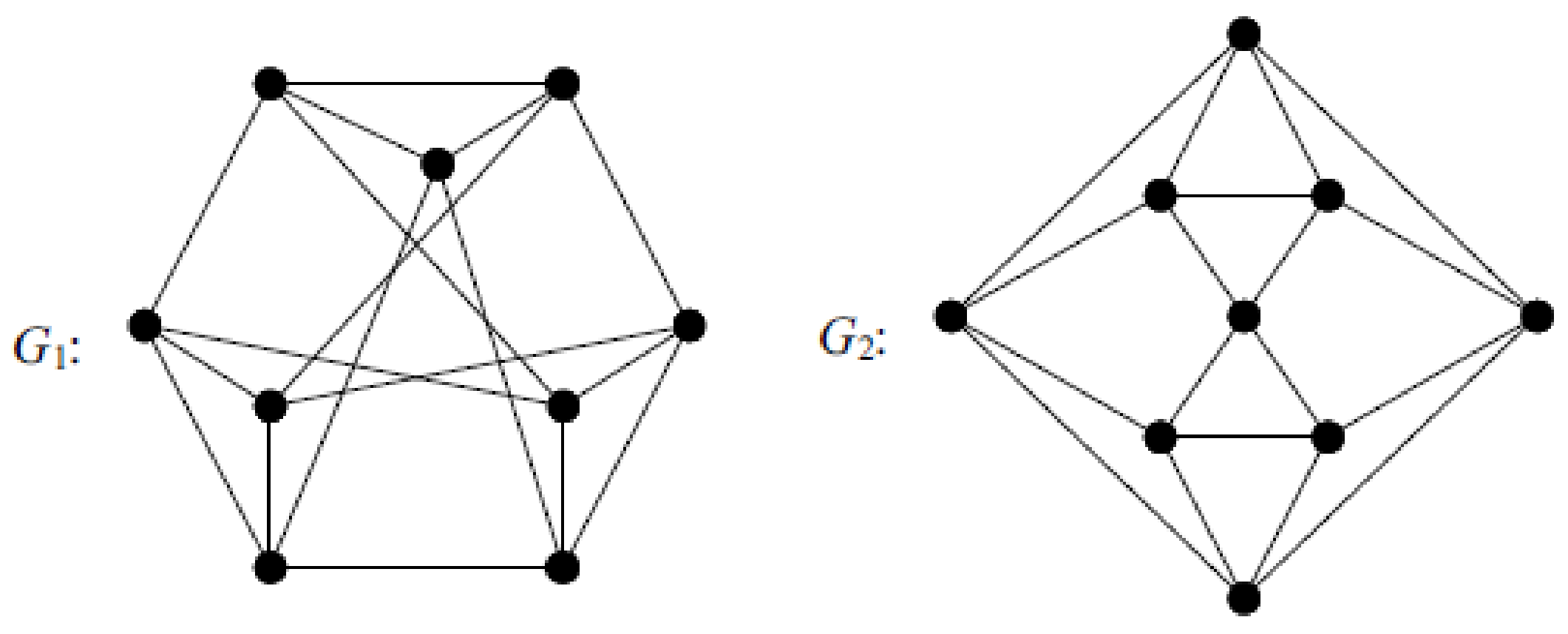
([12]). Let G be an n-vertex r-regular graph with the eigenvalues $r,{\lambda }_2,\dots ,{\lambda }_n$. Then, the eigenvalues of $L\left(G\right)$ are as follows

$$\left.\begin{array}{cc}2r-2and& \\ {\lambda }_i+r-2i=2,\dots ,nand& \\ -2,\frac{n(r-2)}{2}times& \end{array}\right\}$$

(21)

Take into account the graphs $H_1$ and $H_2$ as shown in Figure 1. Let $G_1=L\left(H_1\right)$ and $G_2=L\left(H_2\right)$ (see Figure 2). The characteristic polynomials of $H_1$ and $H_2$ are $\Phi (H_1,\lambda )=(\lambda -3){\lambda }^4(\lambda +3)$ and $\Phi (H_2,\lambda )=(\lambda -3)(\lambda -1){\lambda }^2{(\lambda +2)}^2$, respectively.

On the basis of Lemma 3, we obtain the spectrums of $G_1$ and $G_2$ as

$$Spec\left(G_1\right)=\left(\begin{array}{c}41-2\hfill \\ 144\hfill \end{array}\right)$$

(22)

and

$$Spec\left(G_2\right)=\left(\begin{array}{c}421-1-2\hfill \\ 11223\hfill \end{array}\right)$$

(23)

respectively. It is easy to see that $\epsilon \left(G_1\right)=\epsilon \left(G_2\right)=16$.

Theorem 3.

For all $n\ge 9$, there exists a pair of connected ISI-noncospectral, ISI-equienergetic graphs of order n.

Proof. 

Take into consideration the graphs $G_1$ and $G_2$ as shown in Figure 2. Graphs $G_1$ and $G_2$ are both connected 9-vertex 4-regular graphs. From (22), (23) and Lemma 1, we have ${\epsilon }_{isi}\left(G_1\right)={\epsilon }_{isi}\left(G_2\right)=2\epsilon \left(G_1\right)=32$, and ${\epsilon }_{isi}\left(K_t\right)={(t-1)}^2$.

Then, by Theorem 2, we have

$$\begin{array}{ccc}\hfill {\epsilon }_{isi}(G_1+K_t)& =& {\epsilon }_{isi}(G_2+K_t)\hfill \\ & =& 6(t+4)+\frac{(t-1)(t+8)}{2}+\frac{1}{2}\sqrt{{(t^2+3t-24)}^2+36t{\left(\frac{(t+8)(t+4)}{t+6}\right)}^2}.\hfill \end{array}$$

Hence, $G_1+K_t$ and $G_2+K_t$ are two ISI-noncospectral and ISI-equienergetic graphs for all $n\ge 9$.

This completes the proof. □

Lemma 4

([14]). Let G be an n-vertex $r(r\ge 3)$-regular graph. Then, among the positive eigenvalues of $\overline{L^2\left(G\right)}$, one is equal to the degree of $\overline{L^2\left(G\right)}$, whereas all others are equal to 1.

Lemma 5

([14]). If G is an n-vertex and $r(r\ge 3)$-regular graph, then for $k\ge 2$, among the positive eigenvalues of $\overline{L^k\left(G\right)}$, one is equal to the degree of $\overline{L^k\left(G\right)}$, whereas all others are equal to 1.

Theorem 4.

If G is an n-vertex and $r(r\ge 3)$-regular graph, then

$${\epsilon }_{isi}\left(\overline{L^2\left(G\right)}\right)=\frac{1}{4}(n{r}^2-nr-8r+10)(2n{r}^2-3nr-8r+10).$$

Proof. 

If $\lambda ,{\lambda }_2,\dots ,{\lambda }_n$ are the eigenvalues of an n-vertex $r(r\ge 3)$-regular graph G, then by Lemma 3, the eigenvalues of $L\left(G\right)$ are

$$\left.\begin{array}{cc}2r-2and& \\ {\lambda }_i+r-2i=2,\dots ,nand& \\ -2\frac{n(r-2)}{2}times& \end{array}\right\}$$

(24)

In view of the fact that $L\left(G\right)$ is a $\frac{nr}{2}$-vertex, $(2r-2)$-regular graph, from (24), the eigenvalues of $L^2\left(G\right)$ can be easily calculated as:

$$\left.\begin{array}{cc}{\lambda }_i+3r-6i=1,2,\dots ,nand& \\ 2r-6\frac{n(r-2)}{2}timesand& \\ -2\frac{nr(r-2)}{2}times& \end{array}\right\}$$

(25)

Therefore, from Lemma 2, (24) and (25), we obtain the eigenvalues of $\overline{L^2\left(G\right)}$ as follows:

$$\left.\begin{array}{cc}-{\lambda }_i-3r+5i=2,3,\dots ,nand& \\ -2r+5\frac{n(r-2)}{2}timesand& \\ 1\frac{nr(r-2)}{2}timesand& \\ \frac{nr(r-1)}{2}-4r+5& \end{array}\right\}$$

(26)

Hence, from Lemmas 1 and 4, the ISI-energy of $\overline{L^2\left(G\right)}$ is

$${\epsilon }_{isi}\left(\overline{L^2\left(G\right)}\right)=\frac{1}{2}(\frac{nr(r-1)}{2}-4r+5)\times 2[\frac{nr(r-1)}{2}-4r+5+\frac{nr(r-2)}{2}\times 1]$$

$$=\frac{1}{4}(n{r}^2-nr-8r+10)(2n{r}^2-3nr-8r+10).$$

This completes the proof. □

Theorem 5.

Let $G_1$ and $G_2$ be two n-vertex $r(r\ge 3)$-regular non-cospectral graphs. Then, $\overline{L^2\left(G_1\right)}$ and $\overline{L^2\left(G_2\right)}$ are ISI-noncospectral, ISI-equienergetic, and ${\epsilon }_{isi}(\overline{L^2(G_1)})={\epsilon }_{isi}(\overline{L^2(G_2)})=\frac{1}{4}(n{r}^2-nr-8r+10)(2n{r}^2-3nr-8r+10)$.

Proof. 

The results can be easily obtained from Theorem 4. □

The line graph of an $n_0$-vertex $r_0$-regular graph G is a regular graph of order $n_1=\frac{1}{2}{r}_0{n}_0$ and of degree $r_1=2r_0-2$. Consequently, the order and degree of $L^k\left(G\right)$ are $n_k=\frac{1}{2}{r}_{k-1}{n}_{k-1}$ and $r_k=2r_{k-1}-2$, where $n_i$ and $r_i$ denote the order and degree of $L^i\left(G\right)$$(i=0,1,2,\cdots )$ [13]. Therefore,

$$r_k=2^k{r}_0-2^{k+1}+2$$

(27)

and

$$n_k=\frac{n_0}{2^k}\prod _{i=0}^{k-1}{r}_i=\frac{n_0}{2^k}\prod _{i=0}^{k-1}(2^i{r}_0-2^{i+1}+2)$$

(28)

Theorem 6.

If G is an $n_0$-vertex $r_0(r_0\ge 3)$-regular graph, then for $k\ge 2$,

$${\epsilon }_{isi}\left(\overline{L^k\left(G\right)}\right)=(n_k-r_k-1)(\frac{2n_k{r}_k}{r_k+2}-r_k-1).$$

Proof. 

It is easily seen that $\overline{L^k\left(G\right)}$ is a regular graph of order $n_k$ and degree $\frac{1}{2}{r}_{k-1}{n}_{k-1}-2r_{k-1}+1$. $\overline{L^k\left(G\right)}$ has $\frac{1}{2}{n}_{k-1}(r_{k-1}-2)$ eigenvalues which are equal to 1. By Lemmas 1, 5 and the fact that the order and degree of $L^k\left(G\right)$ are $n_k=\frac{1}{2}{r}_{k-1}{n}_{k-1}$ and $r_k=2r_{k-1}-2$, we have

$${\epsilon }_{isi}\left(\overline{L^k\left(G\right)}\right)=(\frac{1}{2}{r}_{k-1}{n}_{k-1}-2r_{k-1}+1)(r_{k-1}{n}_{k-1}-2r_{k-1}-n_{k-1}+1)$$

$$=\frac{1}{4}(r_{k-1}{n}_{k-1}-4r_{k-1}+2)(2r_{k-1}{n}_{k-1}-4r_{k-1}-2n_{k-1}+2)$$

$$=(n_k-r_k-1)(\frac{2n_k{r}_k}{r_k+2}-r_k-1).$$

This completes the proof. □

Corollary 3.

If G is an $n_0$-vertex $r_0(r_0\ge 3)$-regular graph, then

$${\epsilon }_{isi}\left(\overline{L^k\left(G\right)}\right)=\left(\left[\frac{n_0}{2^k}\prod _{i=0}^{k-1}(2^i{r}_0-2^{i+1}+2)\right]-2^k{r}_0+2^{k+1}-3\right)$$

$$\times \left(\frac{\left[\frac{n_0}{2^k}{\prod }_{i=0}^{k-1}(2^i{r}_0-2^{i+1}+2)\right](2^k{r}_0-2^{k+1}+2)}{2^{k-1}{r}_0-2^k+2}-2^k{r}_0+2^{k+1}-3\right)$$

From Theorem 6 and Corollary 1, we see that for $r_0$-regular graph G of order $n_0$, the ${\epsilon }_{isi}$ of $\overline{L^k\left(G\right)})(k\ge 2)$ is fully determined by $n_0$ and $r_0$. Hence, we arrive at the following result.

Lemma 6.

Let $G_1$ and $G_2$ be two regular graphs of the same order and of the same degree. Then, for any $k\ge 1$, the following holds:

(i)

$\overline{L^k\left(G_1\right)}$ and $\overline{L^k\left(G_2\right)}$ are of the same order and of the same size.

(ii)

$\overline{L^k\left(G_1\right)}$ and $\overline{L^k\left(G_2\right)}$ are ISI-cospectral if and only if $G_1$ and $G_2$ are ISI-cospectral.

Proof. 

Combining the fact that the number of edges of $L^k\left(G\right)$ is equal to the number of vertices of $L^{k+1}\left(G\right)$ and Equations (27) and (28), statement $\left(i\right)$ holds. Statement $\left(ii\right)$ can be obtained directly from Lemma 3.

This completes the proof. □

Theorem 7.

Let $G_1$ and $G_2$ be two non-cospectral regular graphs of the same order and of the same degree $r\ge 3$. Then, for any $k\ge 2$, graphs $\overline{L^k\left(G_1\right)}$ and $\overline{L^k\left(G_2\right)}$ are a pair of ISI-noncospectral and ISI-equienergetic graphs of equal order and of equal size.

Corollary 3 provides a general method for constructing families of ISI-noncospectral, ISI-equienergetic graphs with the same order. In particular, from Theorem 3 and Theorem 3, it is easy to construct a pair of ISI-noncospectral, ISI-equienergetic n-vertex graphs for all $n\ge 9$.

Within Theorem 4, we obtained the expression in terms of n and r for the ISI-energy of the complement of the second iterated line graph of an n-ordered r-regular graph. Similar representations can be attained also for $\overline{L^k\left(G\right)}$, $k\ge 3$, i.e., the ISI-energy of the complement of the k-th iterated line graph, $k\ge 3$, of an n-ordered $r(r\ge 3)$-regular is also completely determined by the parameters n and r. In addition, for any $k>2$, we can simply find a relevant collection of ISI-noncospectral and ISI-equienergetic regular graphs (of degree greater than 3) by constructing the complement of their k-th iterative line graph.

3. Conclusions

Graph energy has a very wide range of applications in the field of chemistry, physics, satellite communication, face recognition, crystallography, etc. It is worth noting that the energy of numerous graphs can be ascertained by making use of their ISI-energy. A notable discovery in graph energy theory is the existence of non-isomorphic and ISI-noncospectral graphs with equal ${\epsilon }_{isi}$-values.

As far as we know, up to the present, researchers have not yet found a systematic approach to construct pairs (or larger families) of ISI-equienergetic graphs. Consequently, obtaining ISI-noncospectral but ISI-equienergetic graphs with the same order is an interesting and useful thing we should do. In this paper, by studying the ISI-characteristic polynomial of a join graph of two regular graphs, we construct pairs of connected, ISI-noncospectral, ISI-equienergetic graphs of order n for all $n\ge 9$. For example, we consider graph $G_1$, $G_2$ in Figure 2 and graph $K_2$. It is easy to obtain that ${\epsilon }_{isi}\left(G_1\right)={\epsilon }_{isi}\left(G_2\right)=32$, and ${\epsilon }_{isi}\left(K_2\right)=1$, then the ISI-energy of $G_1+K_2$ and $G_2+K_2$ are both equal to $\frac{82+\sqrt{4246}}{2}$, i.e., $G_1+K_2$ and $G_2+K_2$ are a pair of ISI-noncospectral, ISI-equienergetic 11-vertex graphs. In addition, for n-vertex $r(r\ge 3)$-regular graph G, and for each $k\ge 2$, we find ${\epsilon }_{isi}\left(\overline{L^k\left(G\right)}\right)$, depending solely on n and r. This result makes it possible to construct pairs of ISI-noncospectra same-order graphs having equal ISI-energies. For example, we consider graphs $H_1$ and $H_2$ as shown in Figure 1, it is easy to check that the ISI-spectrum of $H_1$ and $H_2$ are $\left(\begin{array}{cc}& \frac{9}{2}0-\frac{9}{2}\hfill \\ & 141\hfill \end{array}\right)$ and $\left(\begin{array}{cc}& \frac{9}{2}\frac{3}{2}0-\frac{6}{2}\hfill \\ & 1122\hfill \end{array}\right),$ respectively, i.e., $H_1$ and $H_2$ are ISI-noncospectral graphs. From Lemma 6, we know that $\overline{L^2\left(H_1\right)}$ and $\overline{L^2\left(H_2\right)}$ are also ISI-noncospectral graphs, and ${\epsilon }_{isi}\left(\overline{L^2\left(H_2\right)}\right)={\epsilon }_{isi}\left(\overline{L^2\left(H_2\right)}\right)=220$, i.e., $\overline{L^2\left(H_1\right)}$ and $\overline{L^2\left(H_2\right)}$, are a pair of ISI-noncospectral, ISI-equienergetic graphs. Furthermore, for any $k\ge 3$, by Lemma 6, we know that $\overline{L^k\left(H_1\right)}$ and $\overline{L^k\left(H_2\right)}$ are a pair of ISI-noncospectral, ISI-equienergetic graphs. Our results enable a systematic construction of pairs of ISI-noncospectral graphs of the same order, having equal ISI-energies.

The graph ISI-energy has taken its rise from theoretical chemistry. Trees, chemical trees, unicyclic and bicyclic graphs are common models of chemical structures. Thus, studying the ${\epsilon }_{isi}$ of these graphs, especially constructing ISI-noncospectral and ISI-equienergetic molecular graphs such as chemical trees, unicyclic, bicyclic and other useful graphs, is also an interesting research direction in the future.