A New Fuzzy Extension of the Simple WISP Method

Abstract

The purpose of this article is to introduce to the literature a new extension of the Simple WISP method adapted for utilizing the triangular fuzzy numbers. This extension is proposed to allow the use of the Simple WISP method for addressing decision-making problems related to uncertainties and inaccuracies, as well as for solving problems related to predictions. In addition, this article also discusses the use of linguistic variables to collect the attitudes of the respondents, as well as their transformation into appropriate triangular fuzzy numbers. The article discusses the use of two defuzzification procedures. The first normalization procedure is easy to use, while the second procedure uses the advantages that the application of asymmetric fuzzy numbers gives in terms of analysis. The usability of the proposed extension is presented through two examples.

1. Introduction

Multicriteria decision-making (MCDM) was first used in the 1970s and has been quickly evolving since then. Many significant MCDM approaches have been proposed as a result of rapid development and use for tackling a broad range of decision-making problems [1,2,3,4,5]. Some of the MCDM methods frequently encountered in the literature are as follows; SAW [6], CP [7], ELECTRE [8], AHP [9], TOPSIS [10], PROMETHEE [11], MACBETH [12], MULTIMOORA [13], and ARAS [14].

In addition to the above-mentioned list including well-known and widely utilized MCDM methods, some newly developed MCDM approaches can be also observed, such as EDAS [15], WASPAS [16], WS PLP [17], ARCAS [18], and CoCoSo [19], etc.

The mentioned (ordinary) MCDM methods have been primarily intended for use with crisp numbers. Yet, most of the real-world decision problems include the vagueness and inaccuracy of the data used to address decision-making problems, and often predictions, which cause significant limitations for the use of ordinary MCDM methods.

To solve problems related to inaccuracies, unreliability, and predictions, Zadeh [20] proposed the theory of fuzzy sets enabling a partial membership in a set. After that, Bellman and Zadeh [21] suggested decision-making in a fuzzy context and thus enabled the utilization of MCDM methods for addressing many decision-making issues, and consequently, many influential MCDM methods were adapted to use fuzzy numbers, such as TOPSIS [22], AHP [23], PROMETHEE [24], ARAS [25], and so on.

In addition, the theory of fuzzy sets has been expanded as well. Of the many extensions, only some of the most significant are listed here, such as neutrosophic set [26,27], interval-valued intuitionistic fuzzy sets [28], interval-valued fuzzy sets [29], and intuitionistic fuzzy sets [30].

In 2021, Stanujkic et al. [31] developed a novel MCDM method integrating some approaches implemented in the WASPAS, MULTIMOORA, ARAS, and CoCoSo methods, named Simple Weighted Sum-Product (WISP) method. For this method, so far, a fuzzy extension has not been proposed. However, extensions that allow the use of the WISP method with intuitionistic [32] and neutrosophic [33] sets have already been proposed. Therefore, the main motivation of the paper was to develop a novel fuzzy extension of the Simple WISP method that is able to cope with a variety of MCDM problems.

For that reason, this article proposes and discusses a fuzzy extension of the WISP method that should allow the use of the WISP method with triangular fuzzy numbers. In addition, this article discusses the use of linguistic variables for collecting attitudes of the respondents, as well as their transformation into appropriate triangular fuzzy numbers. The article also discusses the application of two defuzzification procedures. The first defuzzification procedure is easy to use, while the second procedure uses the advantages that the use of asymmetric fuzzy numbers gives in terms of analysis.

Therefore, the article is structured as follows: Some primary concepts in the fuzzy set theory, as well as some topics related to the proposed method, are explained in Section 2. A fuzzy extension of the Simple WISP method is proposed in Section 3. The usability of the developed approach is presented in Section 4. In order to verify the results obtained with the proposed fuzzy extension a comparison with the results obtained using fuzzy TOPSIS was also performed in this section. In Section 5 of the article, conclusions are given.

2. Preliminaries

This section illustrates some primary concepts in the fuzzy set theory, as well as some topics related to the proposed method.

2.1. Primary Concepts and Definitions of a Fuzzy Set

Definition 1.

X shows a nonempty set. A fuzzy subset $\tilde{A}$ of X is described by its membership function ${\mu }_{\tilde{A}}\left(x\right)$ as follows:

$$\tilde{A}=\{\langle x,{\mu }_{\tilde{A}}\left(x\right)\rangle |x\in X\},$$

(1)

where $x\in X$ denotes that x belongs to the nonempty set X, and ${\mu }_{\tilde{A}}\left(x\right):X\to \left[0,1\right]$.

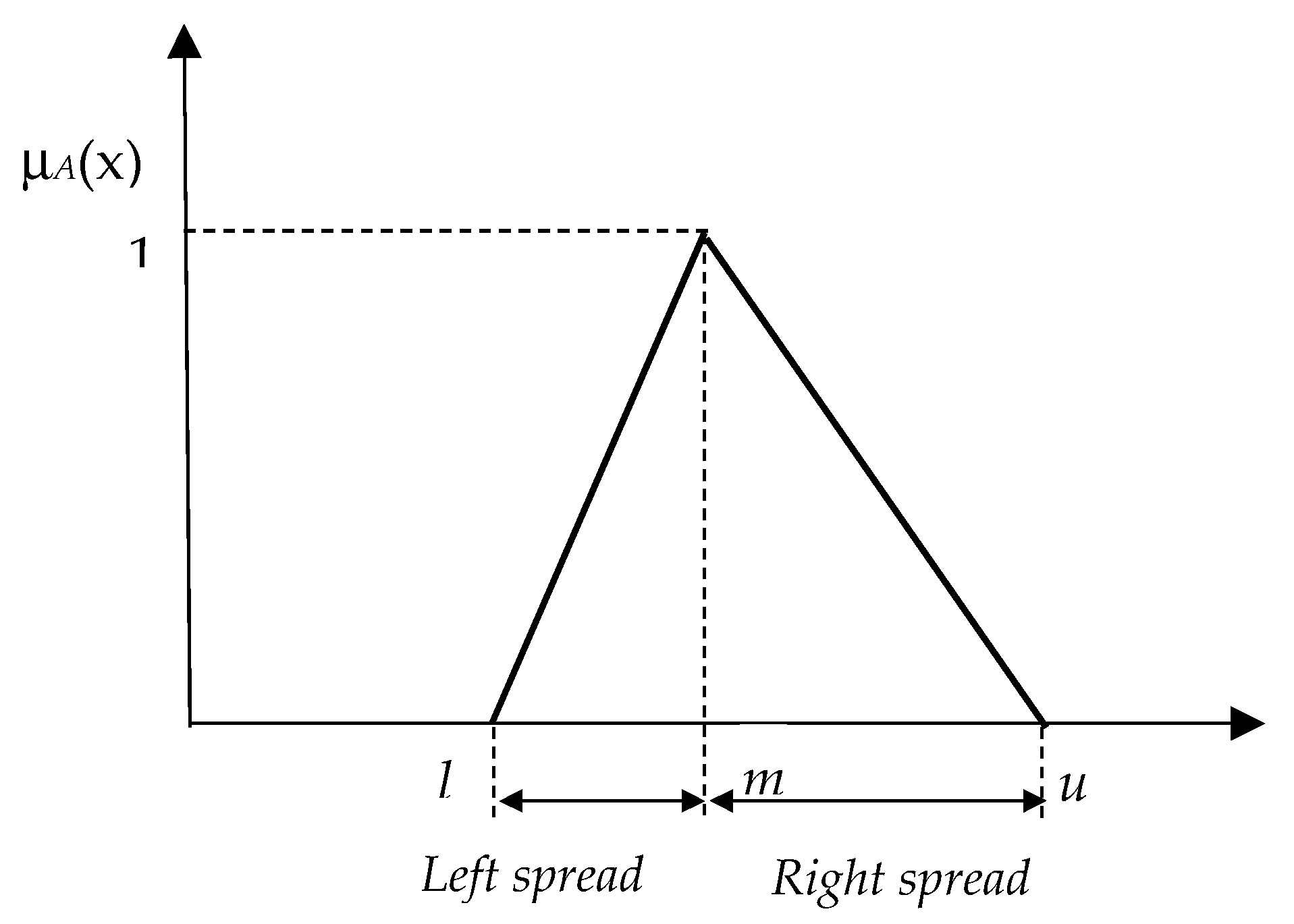
Definition 2.

$\tilde{A}$, which is a fuzzy number, denotes a triangular fuzzy number (TFN) if its membership function is as follows [34]:

$${\mu }_{\tilde{A}}\left(x\right)=\{\begin{array}{ll}\left(x-l\right)/\left(m-l\right)\hfill & l\le x<m\hfill \\ 1\hfill & x=m\hfill \\ \left(u-x\right)/\left(u-m\right)\hfill & m<x\le u\hfill \\ 0\hfill & otherwise\hfill \end{array},$$

(2)

where l, m, and u are left endpoint, mode, and right endpoint, respectively. Triangular fuzzy numbers (TFNs) can also be expressed by their triplets (l, m, u), as shown in Figure 1.

Definition 3.

Let $\tilde{A}=\left(a_l,a_m,a_u\right)$ and $\tilde{B}=\left(b_l,b_m,b_u\right)$ be two positive triangular fuzzy numbers (TFNs), and k denote a non-negative and nonzero crisp number. The basic operations of the above-mentioned TFNs are as follows [35]:

$$\tilde{A}\oplus \tilde{B}=\left(a_l+b_l,a_m+b_m ,a_u+b_u\right),$$

(3)

$$\tilde{A}\ominus \tilde{B}=\left(a_l-b_u,a_m-b_m ,a_u-b_l\right),$$

(4)

$$\tilde{A}\otimes \tilde{B}=\left(a_l · b_l,a_m · b_m ,a_u · b_u\right),$$

(5)

$$\tilde{A}\oslash \tilde{B}=\left(a_l/b_u,a_m/b_m ,a_u/b_l\right),$$

(6)

$$\tilde{A} · k=\left(a_l · k,a_m · k ,a_u · k\right).$$

(7)

$$\tilde{A}+k=\left(a_l+k,a_m+k ,a_u+k\right).$$

(8)

2.2. Defuzzification of Triangular Fuzzy Numbers

Crisp numbers are much more suitable for ranking than fuzzy numbers, which is why fuzzy numbers, just near the end of the evaluation process, are often transformed into crisp numbers before they are ranked. So far, several procedures have been proposed for ranking fuzzy numbers, of which two approaches are mentioned here that will later be used in numerical illustrations.

Opricovic and Tzeng [36] introduced the following defuzzification procedure:

$$df\left(\tilde{A}\right)=\frac{1}{3}\left(l+m+u\right),$$

(9)

where l, m, and u denote the left endpoint, mode, and right endpoint, respectively, of triangular fuzzy number $\tilde{A}$.

In the above procedure, all three points that form a fuzzy number are equally important. The defuzzification procedure proposed by Liou and Wang [37] provides more significant analysis possibilities that could be realized by applying different values of the coefficient λ, and it can be expressed as follows:

$$df\left(\tilde{A}\right)=\frac{1}{2}\left[\left(1-\lambda \right) l+m+\lambda u\right]$$

(10)

where λ denotes the index of optimism, and $\lambda \in \left[0,1\right]$.

When giving a higher value to the index of optimism λ, the value of the right endpoint (optimistic attitudes) has a greater influence on the decision and vice versa; when giving a lower value to the coefficient λ, the left endpoint (pessimistic attitudes) has a greater influence.

2.3. Linguistic Variables

In some cases, the use of fuzzy numbers for evaluating alternatives can be quite complex for respondents who are unfamiliar with the meaning and the use of fuzzy numbers. Therefore, Zadeh [38,39,40] presented the use of linguistic variables in a series of articles, intending to facilitate the use of fuzzy numbers. According to Zadeh, linguistic variables are words or expressions from a natural language whose meaning is associated with the corresponding fuzzy number.

Subsequently, many researchers have applied linguistic variables in their research, such as Chu and Lin [41], Sun and Lin [42], Sun [43], and Shemshadi et al. [44], who have used linguistic variables with fuzzy extensions of the TOPSIS and VIKOR methods.

Certainly, the use of linguistic variables was not limited to the above methods, linguistic variables were also used with other MCDM methods, as well as with other extensions of MCDM methods based on sets derived from fuzzy sets, such as Pythagorean fuzzy sets, interval-valued fuzzy sets, intuitionistic fuzzy sets, and neutrosophic sets. As examples of such recent research, we can mention Karagoz et al. [45] and Gul et al. [46].

Many studies use linguistic scales that are transformed into symmetrical TFN, i.e., fuzzy triangular numbers whose left and right spreads are equal. The use of such fuzzy numbers with simple defuzzification procedures can significantly reduce the benefits that can be achieved by applying fuzzy numbers. Therefore, a different approach for applying the linguistic variables given in

Table 1. The linguistic variables.

Linguistic Variable	Abbreviation	Numeric Value
Extremely high	EHG	9
Very high	VHG	8
High	HG	7
Moderate high	MHG	6
Moderate	M	5
Moderate low	MLW	4
Low	LW	3
Very low	VLW	2
Extremely low	ELW	1

was considered in this article.

In the proposed approach, decision-makers, i.e., respondents, evaluate the alternatives concerning the criteria using the linguistic variables from Table 1. After the evaluation, the linguistic variables are converted into the appropriate crisp numbers.

The further procedure of converting the attitudes of k respondents into an initial group fuzzy decision-making matrix can be shown as follows:

$$l_{ij}=mi{n}_k l_{ij}^k$$

(11)

$$m_{ij}=\frac{1}{K}{\sum }_{k=1}^K{m}_{ij}^k$$

(12)

$$u_{ij}=ma{x}_k u_{ij}^k$$

(13)

where l_ij, m_ij, and u_ij denote the left endpoint, mode, and right endpoint of the fuzzy rating ${\tilde{x}}_{ij}=\left(l_{ij},m_{ij},u_{ij}\right)$ of alternative i concerning the criterion j, and K denotes the number of respondents.

By applying the procedure shown using Equations (11)–(13), fuzzy ratings are obtained, whose left endpoints represent the pessimistic attitudes, whose modes represent the average attitudes, and whose right endpoints represent the optimistic attitudes obtained from the group of respondents, respectively.

3. Fuzzy Simple WISP Method

The procedure of the crisp version of the method (Simple WISP) is given in Stanujkic et al. [31]. Based on this procedure, a procedure can be formed for ranking alternatives in the case of using fuzzy numbers, as follows:

Step 1. Structure a fuzzy initial decision-making matrix and identify criteria weights. In this step, a fuzzy initial decision matrix can be formed as described in Section 2.3, or otherwise. The weights of the criteria can be found using many MCDM methods, such as the SWARA [47], AHP [48], PIPRECIA [49], BWM [50], FUCOM [51] methods, etc.

Step 2. Build a normalized fuzzy decision-making matrix as follows:

$${\tilde{r}}_{ij}={\tilde{x}}_{ij}\frac{1}{{\max }_{i }{u}_{ij}},$$

(14)

where ${\tilde{x}}_{ij}$ denotes a fuzzy rating and ${\tilde{r}}_{ij}$ denotes a normalized fuzzy rating of alternative i with regards to criterion j, respectively.

Step 3. Compute four fuzzy utility measures’ values ${\tilde{u}}_i^{sd}$, ${\tilde{u}}_i^{pd}$, ${\tilde{u}}_i^{sr}$, and ${\tilde{u}}_i^{pr}$, as follows:

$${\tilde{u}}_i^{sd}={\sum }_{j\in {\mathsf{\Omega }}_{\max }}{\tilde{r}}_{ij}{w}_j-{\sum }_{j\in {\mathsf{\Omega }}_{\min }}{\tilde{r}}_{ij}{w}_j,$$

(15)

$${\tilde{u}}_i^{pd}={\prod }_{j\in {\mathsf{\Omega }}_{\max }}{\tilde{r}}_{ij}{w}_j-{\prod }_{j\in {\mathsf{\Omega }}_{\min }}{\tilde{r}}_{ij}{w}_j,$$

(16)

$${\tilde{u}}_i^{sr}=\frac{{\sum }_{j\in {\mathsf{\Omega }}_{\max }}{\tilde{r}}_{ij} w_j}{{\sum }_{j\in {\mathsf{\Omega }}_{\min }}{\tilde{r}}_{ij} w_j}, \mathrm{and}$$

(17)

$${\tilde{u}}_i^{pr}=\frac{{\prod }_{j\in {\mathsf{\Omega }}_{\max }}{\tilde{r}}_{ij }{w}_j}{{\prod }_{j\in {\mathsf{\Omega }}_{\min }}{\tilde{r}}_{ij }{w}_j},$$

(18)

where ${\mathsf{\Omega }}_{min}$ and ${\mathsf{\Omega }}_{max}$ are a set of nonbeneficial and a set of beneficial criteria, respectively.

In Equations (15)–(17), the sum was calculated using Equation (3) and the product using Equation (5).

Step 4. Recalculate the values of the four utility measures as follows:

$${\tilde{\mathit{\upsilon }}}_i^{sd}=\frac{1+{\tilde{u}}_i^{sd}}{1+ma{x}_{i }{u}_i^{sd}},$$

(19)

$${\tilde{\mathit{\upsilon }}}_i^{pd}=\frac{1+{\tilde{u}}_i^{pd}}{1+ma{x}_i u_i^{pd}},$$

(20)

$${\tilde{\mathit{\upsilon }}}_i^{sr}=\frac{1+{\tilde{u}}_i^{sr}}{1+ma{x}_i u_i^{sr}}, \mathrm{and}$$

(21)

$${\tilde{\mathit{\upsilon }}}_i^{pr}=\frac{1+{\tilde{u}}_i^{pr}}{1+ma{x}_i u_i^{pr}},$$

(22)

where ${\tilde{\mathit{\upsilon }}}_i^{sd}$, ${\tilde{\mathit{\upsilon }}}_i^{pd}$, ${\tilde{\mathit{\upsilon }}}_i^{sr}$, and ${\tilde{\mathit{\upsilon }}}_i^{pr}$ denote the recalculated values of ${\tilde{u}}_i^{sd}$, ${\tilde{u}}_i^{pd}$ ${\tilde{u}}_i^{sr}$, and ${\tilde{u}}_i^{pr}$, respectively, and $u_i^{sd}$, $u_i^{pd}$, $u_i^{sr}$, and $u_i^{pr}$ are the supreme values of the right endpoints of four fuzzy utility measures, respectively.

Step 5. Identify the overall fuzzy utility ${\tilde{\mathit{\upsilon }}}_i$ of each alternative as follows:

$${\tilde{\mathit{\upsilon }}}_i=\frac{1}{4}\left({\tilde{\mathit{\upsilon }}}_i^{sd}+{\tilde{\mathit{\upsilon }}}_i^{pd}+{\tilde{\mathit{\upsilon }}}_i^{sr}+{\tilde{\mathit{\upsilon }}}_i^{pr}\right).$$

(23)

Step 6. Identify the crisp overall utility ${\upsilon }_i$ of each alternative. Compared to the ordinary Simple WISP method, the fuzzy extension of this method has one more step, in which fuzzy numbers are transformed into crisp numbers, which can be done by applying Equation (9) or (10).

Step 7. Sort the alternatives and choose the most appropriate one. The alternative with the highest value of ${\upsilon }_i$ is the most suitable one.

4. Numerical Illustrations

In this section, two numerical illustrations are considered. The first illustration refers to the selection of mills for grinding copper ore in copper flotation. This example is borrowed from Stanujkic et al. [52], but it was significantly modified to present the previously discussed methodology. This example demonstrates the use of linguistic variables for evaluating alternatives in group decision-making as well as forming group fuzzy ratings based on crisp ratings obtained from respondents. This example also presents the use of the simpler of the two considered procedures for defuzzification. The results obtained with the proposed extension are also compared with the results obtained using fuzzy TOPSIS.

The second considered example refers to the evaluation of investment projects under uncertainty, which is why net cash flow, i.e., average annual profit, and project risk are presented using triangular fuzzy numbers.

4.1. The First Numerical Illustration

In copper flotations, one of the following three froth flotation circuits is often used for grinding copper ores:

-

Flotation circuits based on rod mills, ball mills, and related equipment (A₁);

-

Flotation circuits based on ball mills and related equipment (A₂);

-

Flotation circuits based on the use of semi-autogenous mills, and related equipment (A₃).

When selecting the most suitable flotation circuits design, in addition to the characteristics of copper ore, it is necessary to take into account the following criteria:

-

GE, grinding efficiency;

-

EE, economic efficiency;

-

TR, technological reliability;

-

CI, capital investment.

To verify the viability of the Fuzzy WISP method, a simulation of the selection of the most suitable flotation circuits design for grinding and froth flotation of ore from an ore deposit located in South and Eastern Serbia was performed. Five experts in extractive metallurgy participated in this simulation, i.e., two from the Technical Faculty in Bor and three from the Mining and Metallurgy Institute Bor. In the simulation, they used the linguistic variables, shown in Table 1, to evaluate three flotation circuits designs mentioned above. The results obtained from the five experts are shown in

Table 2. First expert’s assessments.

	GE	EE	TR	CI
A1	VHG	HG	HG	HG
A2	HG	HG	HG	MHG
A3	MHG	MHG	VHG	MHG

,

Table 3. Second expert’s assessments.

	GE	EE	TR	CI
A1	VHG	HG	HG	MHG
A2	HG	HG	HG	MHG
A3	MHG	HG	VHG	MHG

,

Table 4. Third expert’s assessments.

	GE	EE	TR	CI
A1	EHG	EHG	VHG	MHG
A2	VHG	HG	VHG	HG
A3	VHG	VHG	EHG	VHG

,

Table 5. Fourth expert’s assessments.

	GE	EE	TR	CI
A1	EHG	VHG	VHG	HG
A2	VHG	HG	MHG	HG
A3	HG	HG	EHG	HG

and

Table 6. Fifth expert’s assessments.

	GE	EE	TR	CI
A1	EHG	VHG	VHG	MHG
A2	VHG	HG	HG	HG
A3	HG	EHG	EHG	VHG

.

The group fuzzy decision matrix, formed by transforming linguistic variables into crisp values and applying Equations (11)–(13), is shown in

Table 7. The group fuzzy decision matrix.

	GE	EE	TR	CI
A1	(8.0, 8.6, 9.0)	(7.0, 7.8, 9.0)	(7.0, 7.6, 8.0)	(6.0, 6.4, 7.0)
A2	(7.0, 7.6, 8.0)	(7.0, 7.0, 7.0)	(6.0, 7.0, 8.0)	(5.0, 6.2, 7.0)
A3	(6.0, 6.8, 8.0)	(6.0, 7.6, 9.0)	(8.0, 8.6, 9.0)	(6.0, 7.0, 8.0)

, and the normalized fuzzy decision matrix, formed by applying Equation (14), is shown in

Table 8. Normalized fuzzy decision matrix.

	GE	EE	TR	CI
wj	0.27	0.22	0.22	0.28
optimization	max	max	max	min
A1	(0.89, 0.96, 1.00)	(0.78, 0.87, 1.00)	(0.78, 0.84, 0.89)	(0.75, 0.80, 0.88)
A2	(0.78, 0.84, 0.89)	(0.78, 0.78, 0.78)	(0.67, 0.78, 0.89)	(0.63, 0.78, 0.88)
A3	(0.67, 0.76, 0.89)	(0.67, 0.84, 1.00)	(0.89, 0.96, 1.00)	(0.75, 0.88, 1.00)

.

Table 8 also shows the weights of the criteria and the direction of the optimization of the criteria. Based on Table 8, using Equations (15)–(18), the values of the four utility measures, shown in

Table 9. The values of the four utility measures.

	${\tilde{\mathit{u}}}_{\mathit{i}}^{\mathit{s}\mathit{d}}$	${\tilde{\mathit{u}}}_{\mathit{i}}^{\mathit{p}\mathit{d}}$	${\tilde{\mathit{u}}}_{\mathit{i}}^{\mathit{s}\mathit{r}}$	${\tilde{\mathit{u}}}_{\mathit{i}}^{\mathit{p}\mathit{r}}$
A1	(0.34, 0.41, 0.48)	(−0.24, −0.21, −0.20)	(2.38, 2.83, 3.26)	(0.03, 0.04, 0.06)
A2	(0.28, 0.35, 0.43)	(−0.24, −0.21, −0.17)	(2.15, 2.63, 3.47)	(0.02, 0.03, 0.05)
A3	(0.24, 0.36, 0.47)	(−0.27, −0.24, −0.20)	(1.87, 2.45, 3.24)	(0.02, 0.03, 0.06)

, were calculated.

The recalculated values of the four utility measures, determined using Equations (19)–(22), are shown in

Table 10. The recalculated values of the four utility measures.

	${\tilde{\mathit{\upsilon }}}_{\mathit{i}}^{\mathit{s}\mathit{d}}$	${\tilde{\mathit{\upsilon }}}_{\mathit{i}}^{\mathit{p}\mathit{d}}$	${\tilde{\mathit{\upsilon }}}_{\mathit{i}}^{\mathit{p}\mathit{d}}$	${\tilde{\mathit{\upsilon }}}_{\mathit{i}}^{\mathit{p}\mathit{r}}$
A1	(0.91, 0.96, 1.00)	(0.91, 0.94, 0.96)	(0.76, 0.86, 0.95)	(0.97, 0.99, 1.00)
A2	(0.87, 0.92, 0.97)	(0.91, 0.95, 1.00)	(0.71, 0.81, 1.00)	(0.97, 0.98, 0.99)
A3	(0.84, 0.92, 1.00)	(0.87, 0.92, 0.96)	(0.64, 0.77, 0.95)	(0.97, 0.98, 1.00)

.

Based on Table 10, the overall fuzzy utility of each alternative was calculated using Equation (23) as it is shown in

Table 11. The overall fuzzy utility, overall utility, and ranking order of alternatives.

	${\tilde{\mathit{\upsilon }}}_{\mathit{i}}$	${\mathit{\upsilon }}_{\mathit{i}}$	Rank
A1	(0.888, 0.936, 0.979)	0.234	1
A2	(0.864, 0.913, 0.990)	0.231	2
A3	(0.830, 0.896, 0.977)	0.225	3

. The crisp values of the overall utility of the considered alternatives, calculated using Equation (9), and the ranking order of the alternative are also shown in Table 11.

From Table 11 it can be seen that alternative A₁, i.e., flotation circuits based on rod mills and ball mills, is the most suitable solution for the considered ore deposit. However, the rankings of the alternative concerning l_i, m_i, and u_i of the overall fuzzy utility, shown in

Table 12. The ranking orders based on l_i, m_i, and u_i.

	${\tilde{\mathit{\upsilon }}}_{\mathit{i}}$	Rank li	Rank mi	Rank ui
A1	(0.888, 0.936, 0.979)	1	1	2
A2	(0.864, 0.913, 0.990)	2	2	1
A3	(0.830, 0.896, 0.977)	3	3	3

, show that in the case of rankings based only on u_i, alternative A₂ is the most acceptable.

However, the use of Equation (10) and index of optimism λ = 1 did not cause a change in the ranking order of the alternative because in that case the ranking was done as follows:

$$d{f}_{\lambda =1}\left(\tilde{A}\right)=\frac{1}{2}\left(m+u\right).$$

(24)

The overall fuzzy utility, overall utility, and ranking order of the alternatives obtained using Equation (10) and index of optimism λ = 1 are shown in

Table 13. The overall utility and ranking order of alternatives for λ = 1.

	${\tilde{\mathit{\upsilon }}}_{\mathit{i}}$	${\mathit{\upsilon }}_{\mathit{i}}$	Rank
A1	(0.888, 0.936, 0.979)	0.319	1
A2	(0.864, 0.913, 0.990)	0.317	2
A3	(0.830, 0.896, 0.977)	0.312	3

.

Comparison of the Obtained Results Using the Fuzzy TOPSIS Method

In order to verify the results of the fuzzy extension of the Simple WISP method, the Fuzzy TOPSIS method was applied.

The fuzzy weight-normalized matrix, obtained using the TOPSIS method, is shown in

Table 14. Weighted normalized fuzzy decision matrix.

A1	(0.18, 0.17, 0.17)	(0.13, 0.13, 0.14)	(0.13, 0.12, 0.12)	(0.17, 0.16, 0.15)
A2	(0.15, 0.15, 0.15)	(0.13, 0.12, 0.11)	(0.11, 0.11, 0.12)	(0.14, 0.15, 0.15)
A3	(0.13, 0.14, 0.15)	(0.11, 0.13, 0.14)	(0.14, 0.14, 0.14)	(0.17, 0.17, 0.18)
A+	(0.18, 0.17, 0.17)	(0.17, 0.17, 0.13)	(0.17, 0.13, 0.13)	(0.13, 0.13, 0.14)
A−	(0.13, 0.14, 0.15)	(0.14, 0.15, 0.11)	(0.15, 0.11, 0.12)	(0.11, 0.12, 0.11)

, as well as the ideal and anti-ideal points.

The fuzzy ${\tilde{d}}_i$ and crisp $d_i$ separation measures of each alternative to the ideal and anti-ideal points are shown in

Table 15. Calculation details obtained using fuzzy TOPSIS.

	${\tilde{\mathit{d}}}_{\mathit{i}}^{-}$	${\tilde{\mathit{d}}}_{\mathit{i}}^{+}$	${\mathit{d}}_{\mathit{i}}^{-}$	${\mathit{d}}_{\mathit{i}}^{+}$	${\mathit{C}}_{\mathit{i}}$	Rank
A1	(0.003, 0.002, 0.002)	(0.001, 0.000, 0.000)	0.046	0.024	0.660	1
A2	(0.002, 0.001, 0.000)	(0.002, 0.001, 0.001)	0.031	0.039	0.439	2
A3	(0.001, 0.001, 0.001)	(0.003, 0.002, 0.001)	0.033	0.044	0.430	3

, where the crisp separation measures were calculated on the basis of fuzzy separation measures using Equation (9). Table 15 also shows the relative distance $C_i$ of each alternative to the ideal and anti-ideal solution, as well as the ranks of the alternatives.

As can be seen from Table 15, the ranking order of alternatives obtained using the fuzzy TOPSIS method is identical with the ranking order obtained using the proposed extension of the Simple WISP method, which confirms the correctness of the proposed extension.

4.2. The Second Numerical Illustration

In the second numerical illustration, five investment projects were evaluated based on the following investment criteria:

-

Net present value (NPVA);

-

Internal rate of return (IRRE);

-

Profitability index (PID);

-

Payback period (PBPD);

-

Risk of project failure (RPF).

Due to the use of the proposed extension of the Simple WISP method in this numerical illustration, an evaluation in conditions and uncertainties was applied, which is why the average annual profit and risk of project failure are presented using triangular fuzzy numbers. The basic characteristics of investment projects, that is initial investment (CFo (the values of CFo and CFt are given in millions of euros)). The average annual profit (CFt), project duration (T), and risk of project failure (RPF), relevant for the calculation of NPVA, IRRE, PID, and PBPD, are shown in

Table 16. The basic characteristics of the investment projects.

	A1	A2	A3	A4	A5
CFo	300	350	400	450	500
CFt	(70, 72, 73)	(69, 72, 73)	(97, 99, 101)	(65, 68, 69)	(83, 85, 90)
T	5	6	5	9	8
R	(3.5, 4.0, 4.2)	(3.5, 3.7, 4.0)	(3.7, 3.9, 4.1)	(3.7, 3.9, 4.2)	(3.3, 3.9, 4.5)

.

The values of the evaluation criteria, determined based on the data from Table 16, are shown in

Table 17. The initial decision matrix for the investment projects evaluation.

	NPVA	IRRE	PID	PBPD	RPF
wj	0.26	0.11	0.08	0.29	0.26
optimization	max	max	max	min	min
A1	(3.06, 11.72, 16.05)	(0.05, 0.06, 0.07)	(1.01, 1.04, 1.05)	4	(3.5, 4.0, 4.2)
A2	(0.22, 15.45, 20.53)	(0.05, 0.06, 0.07)	(1.00, 1.04, 1.06)	4	(3.5, 3.7, 4.0)
A3	(19.96, 28.62, 37.28)	(0.07, 0.08, 0.08)	(1.05, 1.07, 1.09)	6	(3.9, 4.1, 4.5)
A4	(12.01, 33.33, 40.44)	(0.06, 0.07, 0.07)	(1.03, 1.07, 1.09)	6	(3.7, 3.9, 4.2)
A5	(3.06, 11.72, 16.05)	(0.05, 0.06, 0.07)	(1.01, 1.04, 1.05)	4	(3.5, 4.0, 4.2)

. The same table also shows the weights of the criteria, determined using the AHP method, as well as the optimization directions.

The decision matrix used for calculating the criteria weights by applying the AHP method is shown in

Table 18. The initial decision matrix used for determining criteria weights.

	NPVA	IRRE	PID	PBPD	RPF	wi
NPVA	1	2	5	1	1	0.26
IRRE	0.50	1	3	0.33	0.11	0.11
PID	0.20	0.33	1	0.50	0.50	0.08
PBPD	1.00	3.00	2.00	1	3.0	0.29
RPF	1.00	9.00	2.00	0.33	1	0.26

. The obtained criteria weights, achieved with a consistency ratio = 2.58%, are also shown in the mentioned table.

The normalized fuzzy decision matrix, formed by applying Equation (14), is shown in

Table 19. Normalized fuzzy decision matrix.

	NPVA	IRRE	PID	PBPD	RPF
wj	0.26	0.11	0.08	0.29	0.26
	max	max	max	min	min
A1	(0.04, 0.14, 0.20)	(0.60, 0.72, 0.78)	(0.87, 0.89, 0.91)	(0.67, 0.67, 0.67)	(0.78, 0.89, 0.93)
A2	(0.00, 0.19, 0.25)	(0.56, 0.72, 0.77)	(0.86, 0.90, 0.91)	(0.83, 0.67, 0.67)	(0.78, 0.82, 0.89)
A3	(0.24, 0.35, 0.46)	(0.76, 0.85, 0.93)	(0.90, 0.92, 0.94)	(0.67, 0.67, 0.50)	(0.87, 0.91, 1.00)
A4	(0.15, 0.41, 0.50)	(0.63, 0.75, 0.78)	(0.88, 0.92, 0.94)	(1.00, 1.00, 1.00)	(0.82, 0.87, 0.93)
A5	(0.45, 0.60, 1.00)	(0.76, 0.83, 1.00)	(0.92, 0.94, 1.00)	(1.00, 1.00, 1.00)	(0.73, 0.87, 1.00)

. The weights of the criteria and the directions of optimization, from Table 17, are also shown in the mentioned table.

The values of the four utility measures, calculated using Equations (15)–(18), are shown in

Table 20. The values of the four utility measures.

	${\tilde{\mathit{u}}}_{\mathit{i}}^{\mathit{s}\mathit{d}}$	${\tilde{\mathit{u}}}_{\mathit{i}}^{\mathit{p}\mathit{d}}$	${\tilde{\mathit{u}}}_{\mathit{i}}^{\mathit{s}\mathit{r}}$	${\tilde{\mathit{u}}}_{\mathit{i}}^{\mathit{p}\mathit{r}}$
A1	(−0.29, −0.24, −0.19)	(−0.05, −0.04, −0.04)	(0.33, 0.44, 0.53)	(0.00, 0.00, 0.01)
A2	(−0.29, −0.21, −0.22)	(−0.05, −0.04, −0.05)	(0.31, 0.49, 0.50)	(0.00, 0.01, 0.01)
A3	(−0.19, −0.17, −0.12)	(−0.04, −0.05, −0.04)	(0.54, 0.60, 0.70)	(0.01, 0.01, 0.02)
A4	(−0.36, −0.26, −0.22)	(−0.07, −0.07, −0.06)	(0.33, 0.50, 0.57)	(0.00, 0.01, 0.01)
A5	(−0.28, −0.20, −0.04)	(−0.08, −0.06, −0.05)	(0.49, 0.62, 0.92)	(0.01, 0.02, 0.04)

.

The recalculated values of the four utility measures, calculated using Equations (19)–(22), are shown in

Table 21. The recalculated values of the four utility measures.

	${\tilde{\mathit{\upsilon }}}_{\mathit{i}}^{\mathit{s}\mathit{d}}$	${\tilde{\mathit{\upsilon }}}_{\mathit{i}}^{\mathit{p}\mathit{d}}$	${\tilde{\mathit{\upsilon }}}_{\mathit{i}}^{\mathit{p}\mathit{d}}$	${\tilde{\mathit{\upsilon }}}_{\mathit{i}}^{\mathit{p}\mathit{r}}$	${\tilde{\mathit{\upsilon }}}_{\mathit{i}}$
A1	(0.74, 0.79, 0.84)	(0.99, 0.99, 1.00)	(0.69, 0.75, 0.79)	(0.96, 0.97, 0.97)	(0.42, 0.87, 0.45)
A2	(0.73, 0.82, 0.81)	(0.99, 1.00, 0.99)	(0.68, 0.77, 0.78)	(0.96, 0.97, 0.97)	(0.42, 0.89, 0.44)
A3	(0.84, 0.86, 0.91)	(1.00, 0.99, 0.99)	(0.80, 0.83, 0.89)	(0.97, 0.97, 0.98)	(0.45, 0.91, 0.47)
A4	(0.67, 0.77, 0.81)	(0.97, 0.97, 0.97)	(0.69, 0.78, 0.82)	(0.96, 0.97, 0.97)	(0.41, 0.87, 0.45)
A5	(0.75, 0.83, 1.00)	(0.96, 0.97, 0.98)	(0.78, 0.84, 1.00)	(0.97, 0.98, 1.00)	(0.42, 0.87, 0.45)

. The overall fuzzy utility of the alternatives, calculated using Equation (23), are also shown in Table 21.

Table 22. The overall utility and ranking orders for different values of λ.

	λ = 0		λ = 0.5		λ = 0.75		λ = 1
	${\mathit{\upsilon }}_{\mathit{i}}$	Rank	${\mathit{\upsilon }}_{\mathit{i}}$	Rank	${\mathit{\upsilon }}_{\mathit{i}}$	Rank	${\mathit{\upsilon }}_{\mathit{i}}$	Rank
A1	0.860	4	0.874	4	0.881	4	0.888	3
A2	0.866	3	0.877	3	0.882	3	0.887	4
A3	0.909	1	0.918	1	0.923	2	0.928	2
A4	0.848	5	0.866	5	0.875	5	0.884	5
A5	0.885	2	0.918	2	0.935	1	0.951	1

shows a case of analyses that can be performed using Equation (10) and different values of the index of optimism λ.

From Table 20 it can be seen that the change in the value of the lambda coefficient affects the order of the ranked alternatives, which can be useful in the case of the analysis of different scenarios.

It is known that the rank of an alternative in MCDM decision-making shows its acceptability, which means that the first-ranked alternative is also the most acceptable alternative. Using the proposed approach, decision-makers can, using different values of the lambda coefficient, consider different scenarios, and depending on their preferences, select the most appropriate alternative.

5. Conclusions

This article presented an extension of the Simple WISP method based on the use of triangular fuzzy numbers. The use of this method for solving two examples did not point to any weaknesses of the mentioned method. Moreover, it showed that the proposed extension can be successfully used for solving decision-making problems related to uncertainty.

The article also presented the use of linguistic variables for collecting respondents’ attitudes, as well as their transformation into appropriate triangular fuzzy numbers. In addition, two normalization procedures were considered in this article. The first defuzzification procedure was easy to use, while the second procedure used the advantages that the use of asymmetric fuzzy numbers provides in terms of analysis. The usability of the proposed extension was presented through two examples at the end of the article.

As a direction for future research, a new extension of the simple WISP method can be developed based on the triangular intuitionistic fuzzy numbers [53].