Software Defects Prediction Based on Hybrid Beetle Antennae Search Algorithm and Artificial Bee Colony Algorithm with Comparison

Abstract

Software defects are problems in software that destroy normal operation ability and reflect the quality of the software. Software fault can be predicted by the software reliability model. In this paper, the hybrid algorithm is applied to parameter estimation in software defect prediction. As a biological heuristic algorithm, BAS (Beetle Antennae Search Algorithm) has fast convergence speed and is easy to implement. ABC (Artificial Bee Colony Algorithm) is better in optimization and has strong robustness. In this paper, the BAS-ABC hybrid algorithm is proposed by mixing the two algorithms and the goal of the proposed method is to improve the convergence and stability of the algorithm. Five datasets were used to carry out the experiments, and the data results showed that the hybrid algorithm was more accurate than the single algorithm, with stronger convergence and stability, so it was more suitable for parameter estimation of the software reliability model. Meanwhile, this paper implemented the comparison between hybrid BAS + ABC and hybrid PSO + SSA, and the result shows that BAS + ABC has better performance both in convergence and stability. The comparison result shows the strong ability in estimation and prediction of software defects hybrid BAS and ABC.

1. Introduction

A software reliability prediction model can be used to predict the failure time and defects of software and plays an important role in the evaluation of software quality. The purpose of software reliability prediction is to discover the faults and their distribution during software testing. By understanding these faults, the software in the actual operation of the fault state and hidden faults can be predicted.

The non-homogeneous Poisson process model is a simple discrete stochastic process with a time-continuous state. It is a common model to describe software reliability, and the Goel-Okumoto model (G-O) is a classic software reliability growth model derived from it [1,2]. The G-O model simplifies SRGM parameters, and it has become a commonly used model in the testing process [3].

The maximum likelihood method and least square method are two of the most common method of parameter estimation, but both are related to probability theory and mathematical statistics characteristics, and this is likely to have broken the constraint condition of software reliability model parameters are estimated. Furthermore, if you encounter more complex model or the failure of large-scale data, neither of these two methods can find the optimal parameter estimator. If the traditional numerical calculation method is adopted, it often faces problems such as non-convergence or over-reliance on initial value in the iterative process. Therefore, it is particularly important to find a better and more effective method of reliability model parameter estimation. In addition to the two-parameter estimation methods above, a new idea is to apply swarm intelligence algorithm to model parameter estimation.

Swarm intelligence optimization is a new heuristic computing method based on the observation and inspiration of the behavior of aggregative organisms. Based on these swarm intelligence optimizations, new [4,5,6] and hybrid algorithms [7,8] are proposed to obtain better solutions.

The Beetle Antennae Search Algorithm (BAS) is an intelligent optimization algorithm proposed by Jiang et al. [9] in 2017 which simulates the search mode of a foraging beetle. The algorithm is easy to implement and has fewer control parameters and a faster speed. In addition, the algorithm does not need to know the specific form of the optimization objective, nor does it need gradient information to achieve efficient optimization. Compared with the particle swarm optimization algorithm, BAS only needs one longhorn, which greatly reduces the amount of computation. Yu et al. [10] fused Particle Swarm Optimization (PSO) with BAS, improved the step size and inertia weight adjustment strategy, and proposed an Improved Antennae Beetle Search (IBAS), which can better solve the global optimal solution and is not easy to fall into the local optimal solution. Jia et al. [11] combined BAS with the Artificial Fish-Swarm Algorithm (AFSA) to transform a single individual into a longhorn whisker group, and combined BAS with the clustering behavior, tail-chasing behavior and random behavior of artificial fish. It could quickly obtain the global optimal value.

The Artificial Bee Colony Algorithm (ABC) is a global optimization algorithm based on swarm intelligence proposed by the Karaboga group in 2005. Its intuitive background is derived from honey-seeking and honey-gathering behaviors of bees. Its advantages are that it uses fewer control parameters and has strong robustness. In each iteration process, global and local optimal solutions will be searched, so the probability of finding the optimal solution is greatly increased. In order to avoid the artificial bee colony algorithm from falling into local optimum, Sun [12] et al. needed to improve its development ability. By referring to the evolutionary mechanism of genetic algorithm, they established a genetic model to carry out genetic operations on the nectar source after adopting the optimal reservation, so as to enrich the diversity of the nectar source. Dai [13] et al. updated the nectar source by introducing an optimal difference matrix, determined the update dimension by means of multidimensional search and the greedy selection and initialized the population by Tent chaotic sequence, which not only improved the convergence speed but also ensured a high probability of optimization. Yu [14] et al. proposed an improved discrete artificial bee colony algorithm, namely the evolutionary bee colony algorithm, which discriminates excellent information according to fitness value and historical evolution degree and integrates crossover operator and mutation operator to continuously evolve nectar source, thus fully excavating the value of bee colony and effectively improving iteration efficiency.

In this paper, the BAS-ABC algorithm is used to find the optimal position of the parameter in the software reliability model, and the time of failures is calculated according to the parameter. The algorithm improvement and hybrid method mentioned above have achieved good results to some extent, but the convergence speed needs to be improved. This paper presents a hybrid algorithm of beetle antennae search algorithm and artificial bee colony algorithm (BAS-ABC). The algorithm first uses BAS to get the optimal adaptive value and location, then sets the nectar source location in ABC as the optimal location of each longhorn, and then ABC.

Compared with PSO and other swarm intelligence algorithms, the BAS algorithm requires only one individual, greatly reduces the amount of computation, is easy to implement, and has faster convergence speed and higher convergence quality. Because the BAS algorithm is more effective than the PSO algorithm, it can approach the optimal solution better and faster by dynamically adjusting the search strategy of step size meanwhile keeping randomness, so it has better convergence.

Because of the strong randomness of PSO, the stability of the algorithm is not enough. Because the randomness of the BAS algorithm in the search process is determined by the changes of left and right whiskers, it is generally stable to approach the optimal solution, thus showing better stability.

Section 2 introduces the relevant basic theories: software reliability and its model, the basic principles of BAS and ABC and the implementation of hybrid algorithm. In Section 3, simulation experiments are performed on the dataset. The parameters of the GO model are predicted and the results are analyzed through five groups of classical software failures. The adaptive function [3] used in this paper is compared with the traditional adaptive function, and the results of different algorithms are compared to testify to the feasibility and effectiveness of the BAS-ABC algorithm, which can effectively avoid the problems of slow algorithm convergence and low initial range accuracy. Finally, Section 4 is discussed and Section 5 is a conclusion.

2. Materials and Methods

2.1. Software Reliability and Model

Software reliability is the probability that a software product can complete a specified function without causing system failure under specified conditions and in a specified time.

Software reliability prediction is mainly achieved through modeling. Software reliability modeling can be used to quantitatively analyze the behavior of software and help develop more reliable software. In this paper, the G-O model of the software reliability model is selected and its parameters are estimated. The estimation function of the GO model for cumulative failures of software systems is as follows:

$$m\left(t\right)=a\left(1-e^{-bt}\right)$$

(1)

where $m\left(t\right)$ is an expected function of failures that will occur at time $t$; $a$ is the total number of expected software failures when the software testing is done; $b$ represents the probability that the undiscovered software failures will be discovered, and $b\in \left(0,1\right)$. It can be seen that the parameters of the GO model are $a$ and $b$, and their selection will affect the accuracy of the model prediction.

2.2. Beetle Antennae Search Algorithm

BAS is an algorithm inspired by the principle of longhorn foraging. Beetles do not know the location of food when foraging, but can only forage according to the strength of the food smell. A beetle has two feelers. If the smell on the left side is stronger than on the right side, the beetle flies to the left, otherwise it flies to the right. The smell of food acts as a function that has a different value at each point in the space. The two whiskers of the beetle can collect the smell value of two points nearby. The purpose of the longicorn beetle is to find the point with the maximum global smell value. Mimicking the behavior of longicorn, we can efficiently conduct function optimization.

For an optimization problem in n-dimensional space, we use $x_l$ to represent the left whisker coordinate, $x_r$ to represent the right whisker coordinate, $x$ to represent the centroid coordinate, and $d_0$ to represent the distance between two whiskers. The ratio of step to distance $d_0$ between two whiskers is a fixed constant:

$$step=c\times d_0$$

(2)

where $c$ is a constant, that is, the big beetle with a long distance between the two whiskers takes a big step, and the small beetle with a short distance between the two whiskers takes a small step. Assuming that the orientation of the longicorn’s head is random after flying to the next step, the orientation of the vector from the right whisker to the left whisker of the longicorn’s whisker is also arbitrary. Therefore, it can be expressed as a random vector:

$$dir=rands\left(n,1\right)$$

(3)

Normalize it:

$$dir=dir/norm\left(dir\right)$$

(4)

Then:

$$x_l-x_r=d_0\times dir$$

(5)

Obviously, $x_l$ and $x_r$ can also be expressed as centers of mass:

$$\begin{array}{c}{x}_l=x+d_0\times \frac{dir}{2}\\ x_r=x-d_0\times dir/2\end{array}$$

(6)

For the function ff to be optimized, calculate the odor intensity values of the left and right whiskers:

$$\begin{array}{c}{f}_{left}=f\left(x_l\right)\\ f_{right}=f\left(x_r\right)\end{array}$$

(7)

If $f_{left}<f_{right}$, in order to explore the minimum value of $f$, the beetle moves the distance step in the direction of the left whisker:

$$x=x+step\times normal\left(x_l-x_r\right)$$

(8)

If $f_{left}>f_{right}$, in order to explore the minimum value of $f$, the beetle moves the distance step in the direction of the right whisker:

$$x=x-step\times normal\left(x_l-x_r\right)$$

(9)

The above two cases can be written as a sign function:

$$\begin{array}{c}x=x-step\times normal\left(x_l-x_r\right)\times sign\left(f_{left}-f_{right}\right) \hfill \\ =x-step\times dir\times sign\left(f\_left-f\_right\right)\hfill \end{array}$$

(10)

where $normal$ is the normalized function.

2.3. Artificial Bee Colony Algorithm

ABC uses fewer control parameters and has strong robustness. In addition, in each iteration process, global and local optimal solutions are searched, so the probability of finding the optimal solution is greatly increased. It is assumed that the solution space of the problem is $D$ dimension, the number of bees gathering and observing is $S_N$, and the number of bees gathering or observing is equal to the number of nectar sources. The location of each nectar source represents a possible solution to the problem, and the nectar quantity of the nectar source corresponds to the fitness of the corresponding solution. A bee gatherer corresponds to a nectar source. The bees corresponding to the ith nectar source search for a new nectar source according to the following formula:

$$x_{id}^{\prime }=x_{id}+{\varnothing }_{id}\left(x_{id}-x_{kd}\right)$$

(11)

where $i=1,2,\dots ,S_N$, $D=1,2,\dots ,D$, ${\varnothing }_{id}$ is a random number in $\left[-1,1\right]$. Then, ABC compares the newly generated possible solution with the original one:

$$\begin{array}{c}new:X_i^{\prime }=\left\{x_{i1}^{\prime },x_{i2}^{\prime },\dots ,x_{iD}^{\prime }\right\}\\ old:X_i=\left\{x_{i1},x_{i2},\dots ,x_{iD}\right\}\end{array}$$

(12)

The greedy selection strategy is adopted to retain a better solution. Each observing bee selects a nectar source according to probability, and the probability formula is:

$$p_i=\frac{fi{t}_i}{{{\displaystyle \sum }}_{j=1}^{S_N}fi{t}_j}$$

(13)

where $fi{t}_i$ is the adaptive value of the possible solution $X_i$.

For the selected nectar source, the observer bees searched for new possible solutions according to the above probability formula. When all the foragers and observers searched the entire search space if the fitness of a nectar source was not improved within a given step, the nectar source was discarded, and the foragers corresponding to the nectar source became scouts, which searched for new possible solutions by the following formula. Among them,

$$x_{id}=x_d^{min}+r\times \left(x_d^{max}-x_d^{min}\right)$$

(14)

where $r$ is a random number in $\left[0,1\right]$, $x_d^{max}$ and $x_d^{min}$ are the lower and upper bounds of the d-dimension. Repeat the operation to reach the maximum number of iterations.

2.4. Construction of Fitness Function

Using an intelligent optimization algorithm to solve the parameter estimation problem of the software reliability model, the most important thing is to construct the adaptive function and take it as the optimization goal of the algorithm. According to the characteristics of the software reliability model, the adaptive value function is constructed according to the principle of the least square method as follows:

$$f_{it}=\frac{\sqrt{{{\displaystyle \sum }}_{i=1}^n{\left[m\left(t_i\right)-m^0\left(t_i\right)\right]}^2}}{n}$$

(15)

where $f_{it}$ represents the distance between the measured value of the number of software faults and the real value. The smaller the distance, the better the estimation and prediction. $m\left(t_i\right)$ and $m^0\left(t_i\right)$ represent the cumulative number and the estimated number of failures found from the start of software testing to time $t_i$. $t_i$ is the moment when the i-th failure occurs. $i=1, 2, 3, \dots , n$. $n$ represents the total number of failures that occurred at the end of the test [3].

This paper cites the fitness function constructed by the literature [3], the formula is:

$$f=\left|b-\frac{n\left(1-e^{-b{t}_n}\right)}{n{t}_n{e}^{-b{t}_n}+\left(1-e^{-b{t}_n}\right){{\displaystyle \sum }}_{i=1}^n{t}_i}\right|$$

(16)

On this basis, the BAS-ABC hybrid algorithm proposed in this paper is used for iterative search. When the end condition is satisfied, $f_{it}$ is used as the fitness function to optimize the algorithm. The optimal search results of parameter $b$ are obtained to predict software defects.

2.5. Implementation of BAS-ABC

In BAS, the longicorn beetle can select the side with a strong smell as the next moving direction by comparing the smell intensity received by the left and right antennae. Since food source search is more directional, the algorithm is able to converge faster. In the conventional ABC algorithm, when hired bees search for new food sources, they randomly select food sources from existing food sources, which will reduce the convergence speed of the algorithm. In order to solve the problem of random evolution direction and slow convergence, BAS is introduced to improve ABC, and the optimal location obtained by BAS is taken as the location of the food source so that the evolution is carried out in a specific direction.

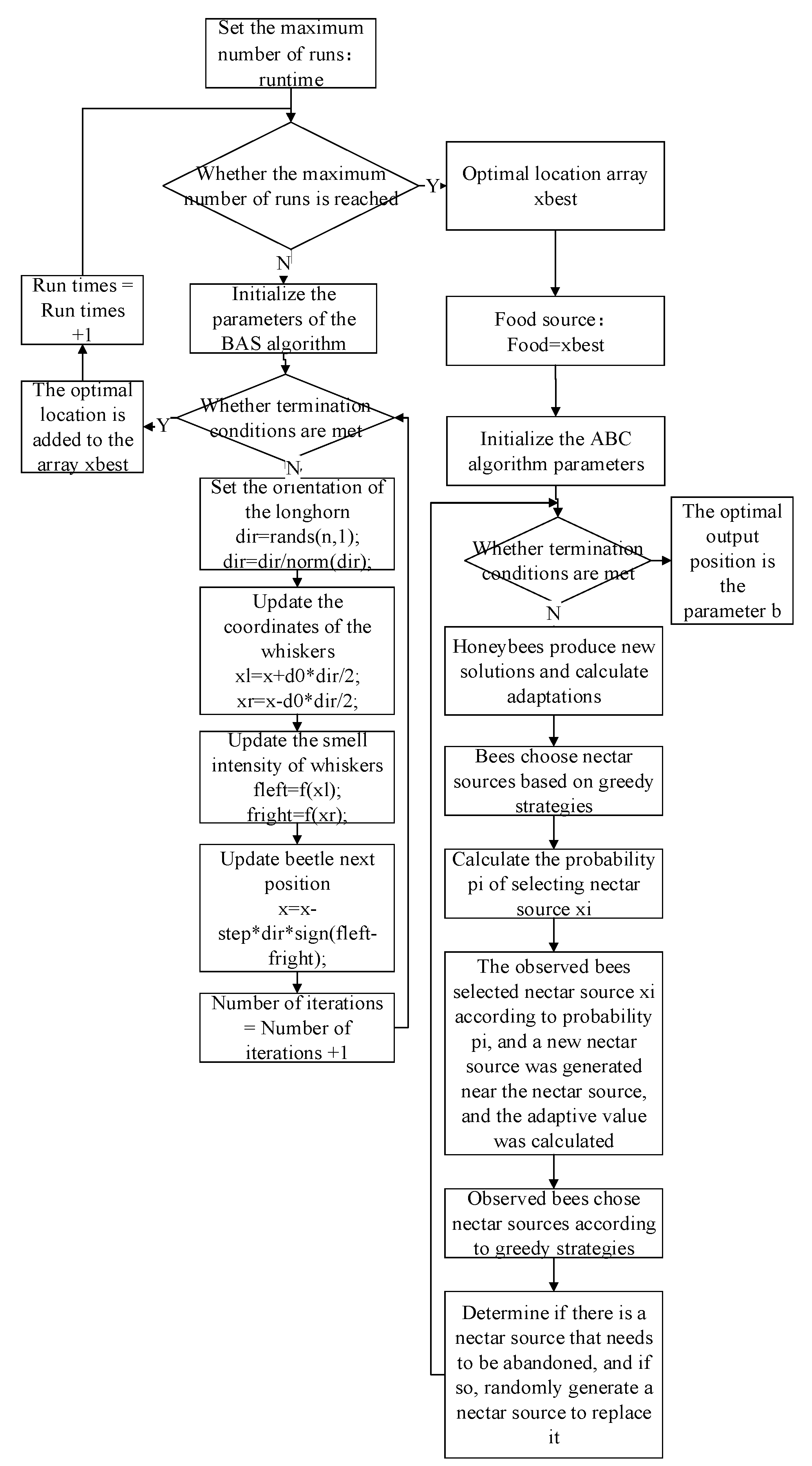
The optimization function f proposed in reference [1] has only one optimal value in the search interval. To speed up the algorithm convergence, this section proposes an algorithm combining BAS and ABC, namely BAS-ABC. The algorithm takes the optimal location as the location of a food source in ABC after obtaining the optimal adaptive value and the optimal location from BAS operation, and the running times of BAS are equal to the number of ABC food sources. The algorithm flow is shown in Figure 1:

Input:

✧

The total quantities of software failures n-10 and the occurrence time $t_i$ of each failure;

✧

The initial parameters of the BAS-ABC algorithm.

Output:

✧

The optimal position and the optimal fitness value are obtained by the BAS-ABC algorithm, and the optimal position is the estimated value of parameter b;

✧

The time of the next ten failures is predicted according to parameter b, and then the difference between the predicted value and the actual value and the root mean square error are calculated, which are represented by error_1 and RMSE, respectively.

(1)

Set the maximum times of BAS algorithm $\mathrm{runtime} =10$, the running times $\mathrm{r}=1$, and the optimal position array $\mathrm{xbest}$.

(2)

Determine whether the maximum number of runs reaches runtime, that is, determine whether $\mathrm{r}> \mathrm{runtime}$ is satisfied. If not, go to Step (3); otherwise, go to Step (10).

(3)

Initialize parameters of BAS algorithm, the step length of beetle: $\mathrm{step}=0.1$, the maximum number of iterations: $\mathrm{n}=10$, the ratio between step and $\mathrm{d}\_0: \mathrm{c}=5$, the coefficient of variable step size: $\mathrm{eta}=0.95$, the number of iterations $\mathrm{iter}=1$.

(4)

Determine whether the termination condition is met, that is $\mathrm{iter}>\mathrm{n}$ or $\mathrm{fbest} <0.0001$. If so, go to Step (8); otherwise, go to Step (5).

(5)

Set the orientation of longicorn beetles.

(6)

Update the coordinate of whiskers, the smell intensity of whiskers, and the next position of the longicorn.

(7)

Iterations +1: $\mathrm{iter}=\mathrm{iter}+1$, go to Step (4).

(8)

Save the optimal position in the array $\mathrm{xbest}$.

(9)

Run times +1: $\mathrm{r}=\mathrm{r}+1$, go to Step (2).

(10)

After the BAS algorithm runs, the optimal location array $\mathrm{xbest}$ is obtained, and the food source of the ABC algorithm $\mathrm{Food}= \mathrm{xbest}$.

(11)

Initialize the parameters of the ABC algorithm, the size of a bee colony: $\mathrm{NP}=20$, the maximum number of iterations: $\mathrm{M}=10$, the number of food: $\mathrm{Food} \mathrm{Number}=10$, the maximum number of searches for a nectar source: $\mathrm{limit}=10$, the upper and lower limits of parameters: $\left(0,1\right)$, the number of iterations $\mathrm{iter}=1$.

(12)

Determine whether the termination conditions are met. If the termination conditions are met $\mathrm{iter}>\mathrm{M}$, go to Step (18); otherwise, go to Step (13).

(13)

Honeybees generate new solutions, calculate adaptations, and select food sources based on greedy strategies.

(14)

Calculate the probability $p_i$ of selecting nectar source $x_i$.

(15)

Observed bees select nectar source $x_i$ according to probability $p_i$ generate a new nectar source near the nectar source, calculate the adaptation value, and selected the nectar source according to the greedy strategy.

(16)

Determine whether there is a nectar source to be abandoned. If there is, a nectar source will be randomly generated to replace it.

(17)

Iterations +1: $\mathrm{iter}=\mathrm{iter}+1$, go to Step (12).

(18)

After the ABC algorithm runs, the optimal position $\mathrm{globalBest}$ is obtained, which is the desired parameter b.

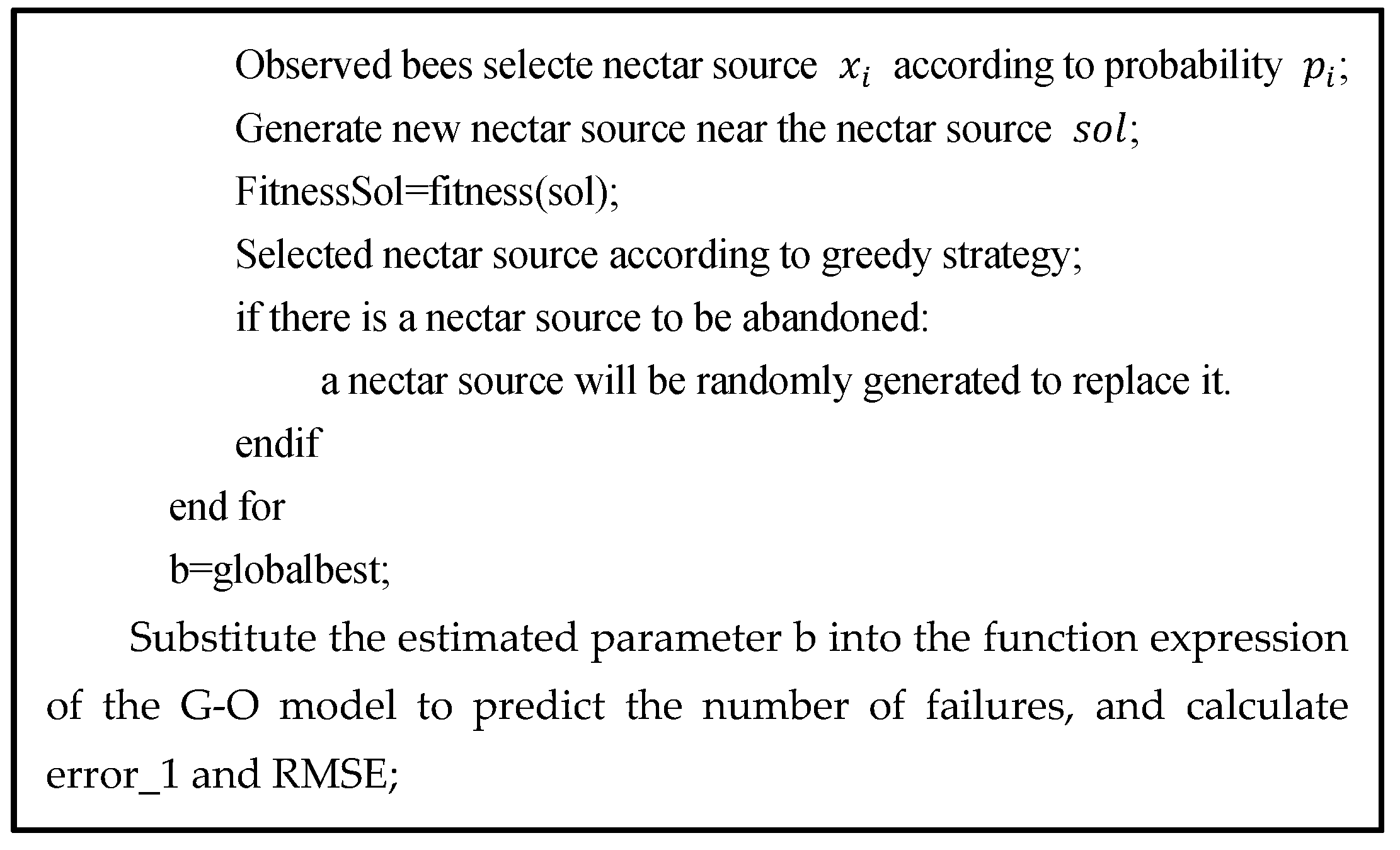
In order to show the steps of the hybrid algorithm more clearly, the algorithm architecture is expressed in interpretable code as Figure 2:

As shown in the interpretable code, the time complexity of BAS-ABC is $O\left(F\times M_1+F\times M_2\right)$, where $F$ represents the running times of the BAS algorithm, that is, the number of honey sources in the ABC algorithm. $M_1$ and $M_2$ represents the maximum number of iterations in the BAS and ABC algorithms. Therefore, according to the calculation principle of algorithm time complexity, the time complexity of BAS-ABC is $O\left(n^2\right)$.

3. Results

The experimental data selected in this paper come from five software failure interval data sets SYS1, SS3, CSR1, CSR2 and CSR3 obtained from actual industrial projects. The address of the data downloaded on is http://www.cse.cuhk.edu.hk/lyu/book/reliability/data.html [15] (accessed on 1 March 2021). Assuming that the actual number of failures of each data set is $\mathrm{n}$, the method adopted in this paper is to estimate model parameters according to the first $n-10$ data, build a software reliability model, and predict the occurrence time of the last 10 failures according to the estimated results, and calculate the predicted performance indicators by comparing with the actual occurrence time.

3.1. Comparison of Three Algorithms

Reference [1] has verified that function f can speed up convergence and improve stability. This section compared the experimental results of the three algorithms—BAS, ABC and BAS-ABC—on the basis of using function f. The parameters of the BAS-ABC algorithm were set as shown in Section 2E, and the parameters of BAS, ABC and hybrid algorithms were set as follows:

• BAS:

  ✧

  The step length of the beetle: $step=0.00001$;

  ✧

  The maximum number of iterations: $n=10$;

  ✧

  The ratio between step and $d_0$: $c=5$;

  ✧

  The coefficient of variable step size: $eta=0.95$.

• ABC:

  ✧

  The size of bee colony: $NP=20$;

  ✧

  The maximum number of iterations: $M=10$;

  ✧

  The number of food: $FoodNumber=10$;

  ✧

  The maximum number of searches for a nectar source: $limit=10$;

  ✧

  The upper and lower limits of parameters: $\left(0,1\right)$.

3.1.1. Fitting and Prediction

In order to observe the results of model fitting and failure number prediction, and to compare the differences between the predicted value and the real value of the three algorithms, this section uses the three algorithms to estimate parameter $b$. After obtaining the optimal parameter $b$, the maximum likelihood formula is used to calculate parameter $a$. According to these two parameters, this paper has drawn the failure times estimation curve in Figure 3, Figure 4, Figure 5, Figure 6 and Figure 7:

From Figure 3, Figure 4, Figure 5, Figure 6 and Figure 7, the red curve represents the actual number of failures with occurrence time. The curve of the BAS-ABC hybrid algorithm is closer to the actual curve than a single algorithm, indicating that the number of failures and occurrence time estimated by the hybrid algorithm is closer to the real value, and indicating that the hybrid algorithm improves the accuracy of the algorithm results.

3.1.2. Data Analysis

To make a comparison between the convergence and stability of the single algorithm and the hybrid algorithm, the three algorithms were repeatedly run 20 times. We have done 10, 20, 40 and 80 times of convergence and stability experiments. From the experimental results, we can see that the algorithm can get the optimal solution of convergence in the case of fewer than 20 operations. Therefore, the algorithm running 20 times is effective and representative in terms of convergence results. At the same time, the experimental results of 20, 40, and 80 times of algorithm stability have little difference and have the same error distribution and stability comparison results. Therefore, the algorithm running 20 times is also effective and representative of the stability results.

The three algorithms were run twenty times on five datasets. The maximum and minimum values of $y$, $error\_1$ and $RMSE$, and the mean values of $y$ are displayed in

Table 1. The best and worst values of different algorithms.

Data Sets	Algorithms	$\mathbf{Fitness} \mathbf{Value} \left(\mathit{y}\right)$			Difference $(\mathit{E}\mathit{r}\mathit{r}\mathit{o}\mathit{r}\_1)$		Root Mean Square $\left(\mathit{R}\mathit{M}\mathit{S}\mathit{E}\right)$
		The Worst	The Best	Average	The Worst	The Best	The Worst	The Best
SYS1	BAS	6.169	0.610	0.888	1.000	0.869	6.205	4.685
	ABC	1.353	0.610	0.653	0.974	0.870	5.560	2.053
	BAS-ABC	0.665	0.610	0.614	0.889	0.833	3.366	1.573
SS3	BAS	9.338	0.611	1.150	1.000	0.433	6.205	1.226
	ABC	7.995	0.611	1.109	1.000	0.336	6.205	1.224
	BAS-ABC	0.776	0.611	0.624	0.480	0.336	2.632	1.215
CSR1	BAS	1.345	1.182	1.284	0.889	0.851	5.809	5.668
	ABC	1.368	1.182	1.197	0.911	0.739	5.891	5.192
	BAS-ABC	1.189	1.182	1.191	0.916	0.720	5.800	5.154
CSR2	BAS	6.258	0.737	1.013	1.000	0.078	6.205	4.446
	ABC	0.927	0.737	0.753	0.649	0.049	5.590	4.386
	BAS-ABC	0.771	0.737	0.740	0.393	0.018	5.090	4.321
CSR3	BAS	1.452	0.766	1.011	0.787	0.643	2.922	1.043
	ABC	1.306	1.118	1.161	0.887	0.876	4.556	4.389
	BAS-ABC	0.571	0.569	0.569	0.670	0.601	1.205	0.983

.

Table 1 compares the differences between the operation results of the three algorithms, and the maximum number of iterations is 10. As can be seen from the above table, the results obtained by the BAS-ABC hybrid algorithm after running are all less than or equal to those obtained by the BAS algorithm and the ABC algorithm alone, indicating that the results obtained by the hybrid algorithm are superior to those obtained by the single algorithm. The data of the minimum value and average value show that the BAS-ABC algorithm has higher accuracy and faster convergence speed, which reflects the accuracy and rapidity in solving the optimal value.

3.1.3. Analysis of Convergence

In the previous section, through numerical analysis, it can be concluded that the BAS-ABC hybrid algorithm has a faster convergence speed. In order to further analyze its convergence, the optimal value obtained by each iteration of the three algorithms is compared, respectively, and the maximum number of iterations is 10. The change of $y$ value of the three algorithms with the number of iterations is shown in Figure 8, Figure 9, Figure 10, Figure 11 and Figure 12:

All three algorithms perform an iterative search on function f to obtain the best estimate of parameter b. As can be seen from Figure 8, Figure 9, Figure 10, Figure 11 and Figure 12, the $y$ value of the hybrid algorithm has converged near the optimal value at the beginning of convergence. Although this is the convergence result of the hybrid algorithm on function $f$, it also indicates that the convergence speed of the hybrid algorithm is indeed higher than that of the single algorithms. Moreover, even though the hybrid algorithm is near the optimal solution, it can still converge rapidly. Since the $y$ value of the hybrid algorithm is already the relative optimal value at the beginning of the iteration, with the continuous convergence of the algorithm, the final result of the hybrid algorithm should be stable to the optimal value.

In addition, the running time of the three algorithms running 20 times is compared, and the results are shown in

Table 2. The running time of the three algorithms running 20 times.

Datasets	Algorithms	Time (Unit: s)
SYS1	BAS	0.716962
	ABC	1.581036
	BAS-ABC	0.501799
SS3	BAS	0.767621
	ABC	2.718816
	BAS-ABC	0.617257
CSR1	BAS	0.865657
	ABC	1.947894
	BAS-ABC	0.589794
CSR2	BAS	0.896610
	ABC	1.854157
	BAS-ABC	0.560032
CSR3	BAS	0.928719
	ABC	1.972067
	BAS-ABC	0.595420

:

It can be found from the table that when the number of runs and iterations are the same, the running time of the hybrid algorithm is less than that of a single algorithm. BAS-ABC has the characteristics of fast running speed. In addition, because of the characteristics of fast convergence and running speed, the BAS-ABC algorithm can converge in fewer iterations, and there is still a short running time in the iterations after convergence, and the iteration duration is shorter than that of a single algorithm.

3.1.4. Analysis of Stability

In order to more intuitively analyze the stability differences of the three algorithms, the maximum iteration number of the algorithm is set to 10 in this section, and the results of running the three algorithms 20 times are compared respectively. Figure 13, Figure 14, Figure 15, Figure 16 and Figure 17 display the data distribution for each dataset:

In Figure 13, Figure 14, Figure 15, Figure 16 and Figure 17, the $y$ value corresponding to the light blue line at the bottom is the optimal value obtained by the algorithm. The distance between the line and other curves represents the difference between the result obtained during each operation of the algorithm and the optimal value. The smaller the difference value is, the closer the result obtained is to the optimal value, indicating the better stability of the algorithm. As can be seen from the above five figures, the distance between the red curve and a horizontal straight line is the smallest, that is, the hybrid algorithm of BAS and ABC has higher stability.

3.2. Comparison with Hybrid PSO and SSA

In this section, the experimental results of BAS-ABC and PSO-SSA algorithms are compared, and the adaptive value function is $f$. The parameters settings of the BAS-ABC algorithm have been introduced in Section 2.5, and the parameters setting of PSO-SSA algorithms are as follows:

• PSO-SSA:

  ✧

  The quantity of particles: $pop=10$;

  ✧

  The maximum number of iterations: $M=10$;

  ✧

  The proportion of explorers is 20%;

  ✧

  The proportion of sparrows aware of danger is 20%;

  ✧

  The safety threshold is 0.8;

  ✧

  The learning factor: $c_1=c_2=1.5$;

  ✧

  The inertia weight: $w=0.9$;

  ✧

  The position of each particle, the parameter b of the G-O model, is initialized to a random number between $\left(0,1\right)$;

  ✧

  The speed is initialized to a random number between $\left[-1,1\right]$.

3.2.1. Fitting and Prediction

In order to intuitively observe the results of model fitting and failure number prediction, and to compare the gap between the predicted value and the real value of the three algorithms, this section uses the two-hybrid algorithms to estimate parameter $b$ and then the maximum likelihood formula is used to calculate parameter $a$. According to $a$ and $b$, the estimated curve of software failure numbers with the time of failure occurrence can be drawn. The model results and actual software failures of the two algorithms are shown in Figure 18, Figure 19, Figure 20, Figure 21 and Figure 22:

From Figure 18, Figure 19, Figure 20, Figure 21 and Figure 22, the red curve represents the actual number of failures over time. The BAS-ABC estimation prediction curve analysis proposed in this paper is closer to the actual curve than the PSO-SSA algorithm, which shows that the BAS-ABC hybrid algorithm improves the accuracy of the algorithm results.

3.2.2. Data Analysis

To make a comparison of the convergence and stability of the two-hybrid algorithms, the two algorithms were repeatedly run 20 times. The maximum and minimum values of $y$, $error\_1$ and $RMSE$, and the mean values of $y$ are shown in

Table 3. The best and worst values of different algorithms.

Data Sets	Algorithms	$\mathbf{Fitness} \mathbf{Value} \left(\mathit{y}\right)$			Difference $(\mathit{E}\mathit{r}\mathit{r}\mathit{o}\mathit{r}\_1)$		Root Mean Square $\left(\mathit{R}\mathit{M}\mathit{S}\mathit{E}\right)$
		The Worst	The Best	Average	The Worst	The Best	The Worst	The Best
SYS1	PSO-SSA	2..279	0.610	0.944	0.992	0.872	5.097	2.972
	BAS-ABC	0.618	0.610	0.611	0.885	0.863	3.176	2.497
SS3	PSO-SSA	1.602	0.611	1.024	0.690	0.472	5.967	1.289
	BAS-ABC	0.679	0.611	0.617	0.500	0.440	1.553	1.236
CSR1	PSO-SSA	2.811	1.182	1.415	0.997	0.854	6.198	5.732
	BAS-ABC	1.267	1.182	1.193	0.898	0.787	5.842	5.420
CSR2	PSO-SSA	1.723	0.740	0.957	0.965	0.658	5.592	4.134
	BAS-ABC	0.801	0.737	0.743	0.381	0.296	5.066	3.658
CSR3	PSO-SSA	0.857	0.611	0.760	0.971	0.790	5.54	4.418
	BAS-ABC	0.596	0.571	0.575	0.671	0.620	1.180	0.984

.

Table 2 compares the difference in the operational results of the two algorithms, and the maximum number of iterations is 10. It can be seen from the above table that the results obtained by the BAS-ABC hybrid algorithm are less than or equal to the results obtained by the PSO-SSA hybrid algorithm, indicating that the BAS-SSA hybrid algorithm proposed in this paper is better than the PSO-SSA hybrid algorithm. The results were obtained. It can be seen from the data of the minimum value and the average value that the BAS-SSA hybrid algorithm has higher accuracy and faster convergence speed, which reflects the accuracy and speed of solving the optimal value.

3.2.3. Analysis of Convergence

In the Section 3.1.3, it can be concluded that the BAS-ABC hybrid algorithm converges faster through numerical analysis. In order to further analyze its convergence, the optimal values obtained by each iteration of the two algorithms were compared, and the maximum number of iterations was 10. The change of the $y$ value of the two algorithms with the number of iterations is shown in Figure 23, Figure 24, Figure 25, Figure 26 and Figure 27:

Both algorithms optimize the function $f$, and the resulting optimal position is used as an estimate of parameter $b$. From Figure 23, Figure 24, Figure 25, Figure 26 and Figure 27, it can be seen that the y value of the BAS-ABC hybrid algorithm converges near the optimal value at the beginning of the convergence, indicating that the convergence speed of the BAS-ABC hybrid algorithm is indeed higher than that of the PSO-SSA hybrid algorithm. Moreover, even though the BAS-ABC hybrid algorithm is close to the optimal solution, it can still converge quickly. Since the $y$ of the BAS-ABC hybrid algorithm is already a relatively optimal value at the beginning of the iteration, as the algorithm continues to converge, the final result of the BAS-ABC hybrid algorithm should stabilize at the optimal value.

3.2.4. Analysis of Stability

In order to more intuitively analyze the stability differences of the three algorithms, the maximum iteration number of the algorithm is set to 10 in this section, and the results of running the three algorithms 20 times are compared respectively. Figure 28, Figure 29, Figure 30, Figure 31 and Figure 32 display the data distribution for each dataset:

As can be seen in Figure 27, Figure 28, Figure 29, Figure 30 and Figure 31, the distance between the red curve and the horizontal line is smaller than the distance between the blue curve and the horizontal line, indicating that the BAS-ABC is more stable than the PSO-SSA.

4. Discussion

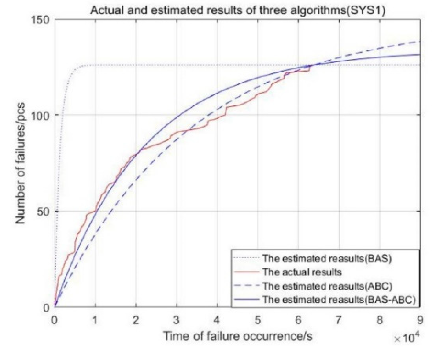
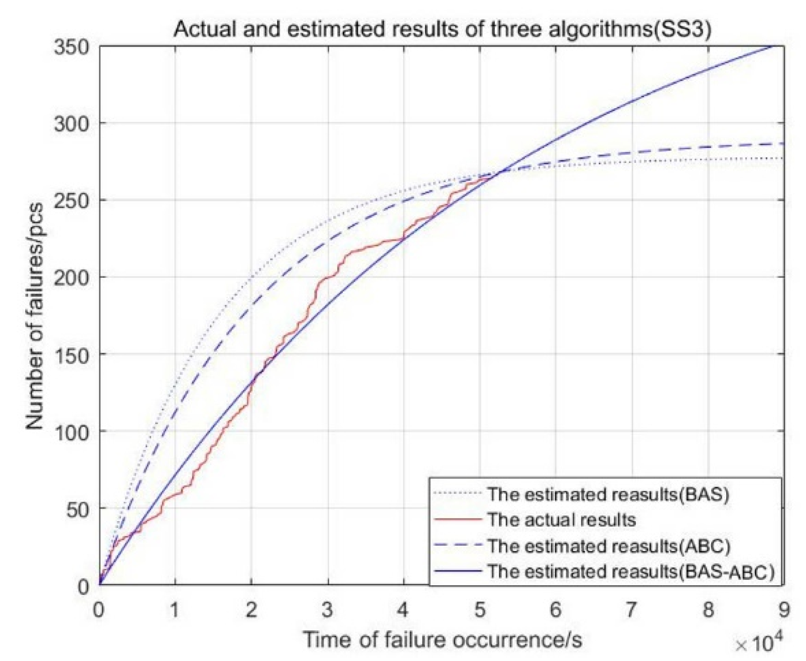
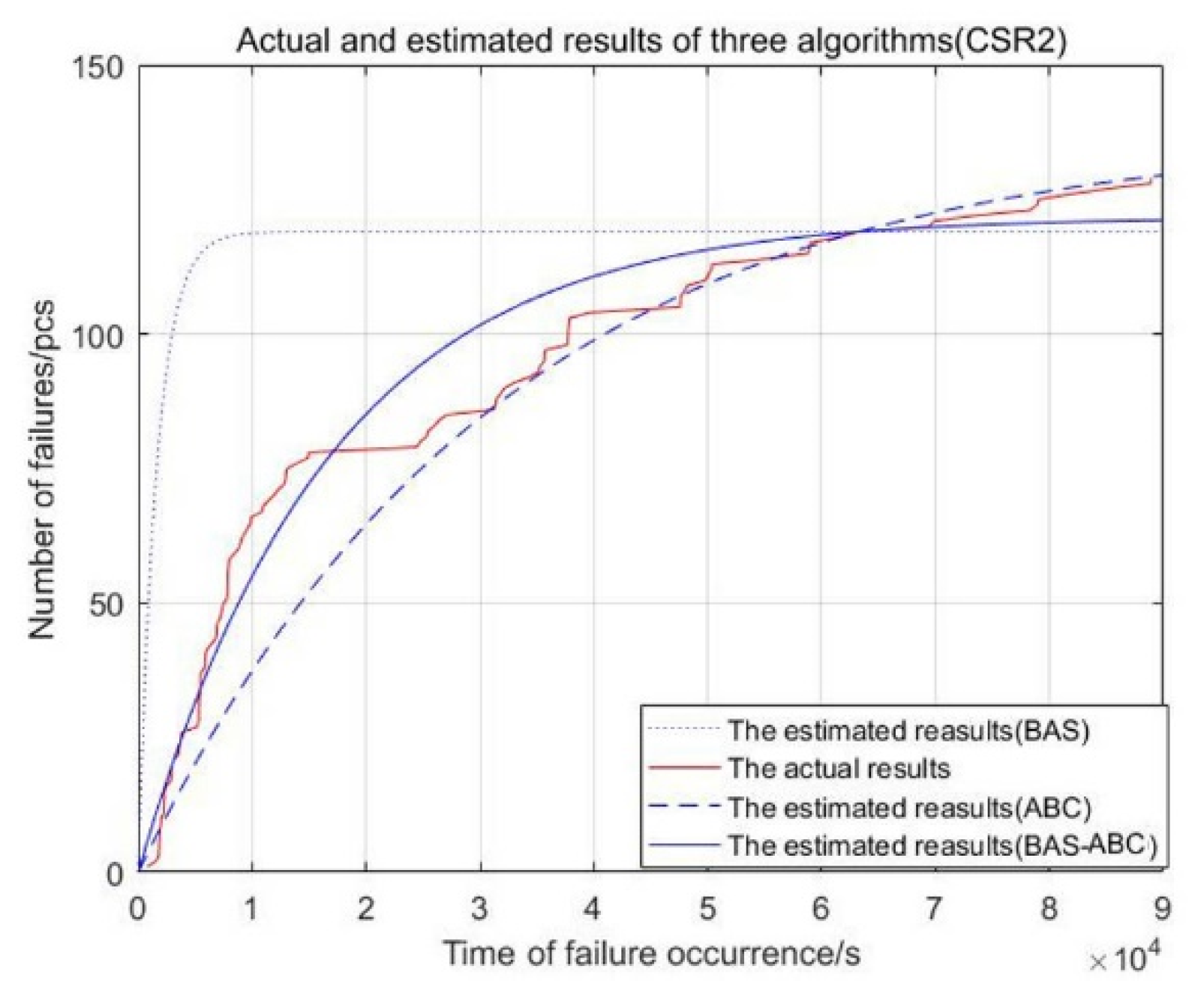
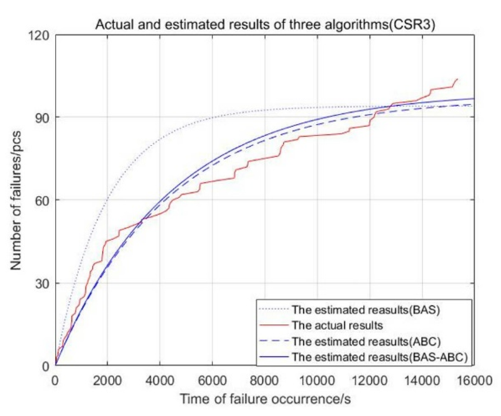
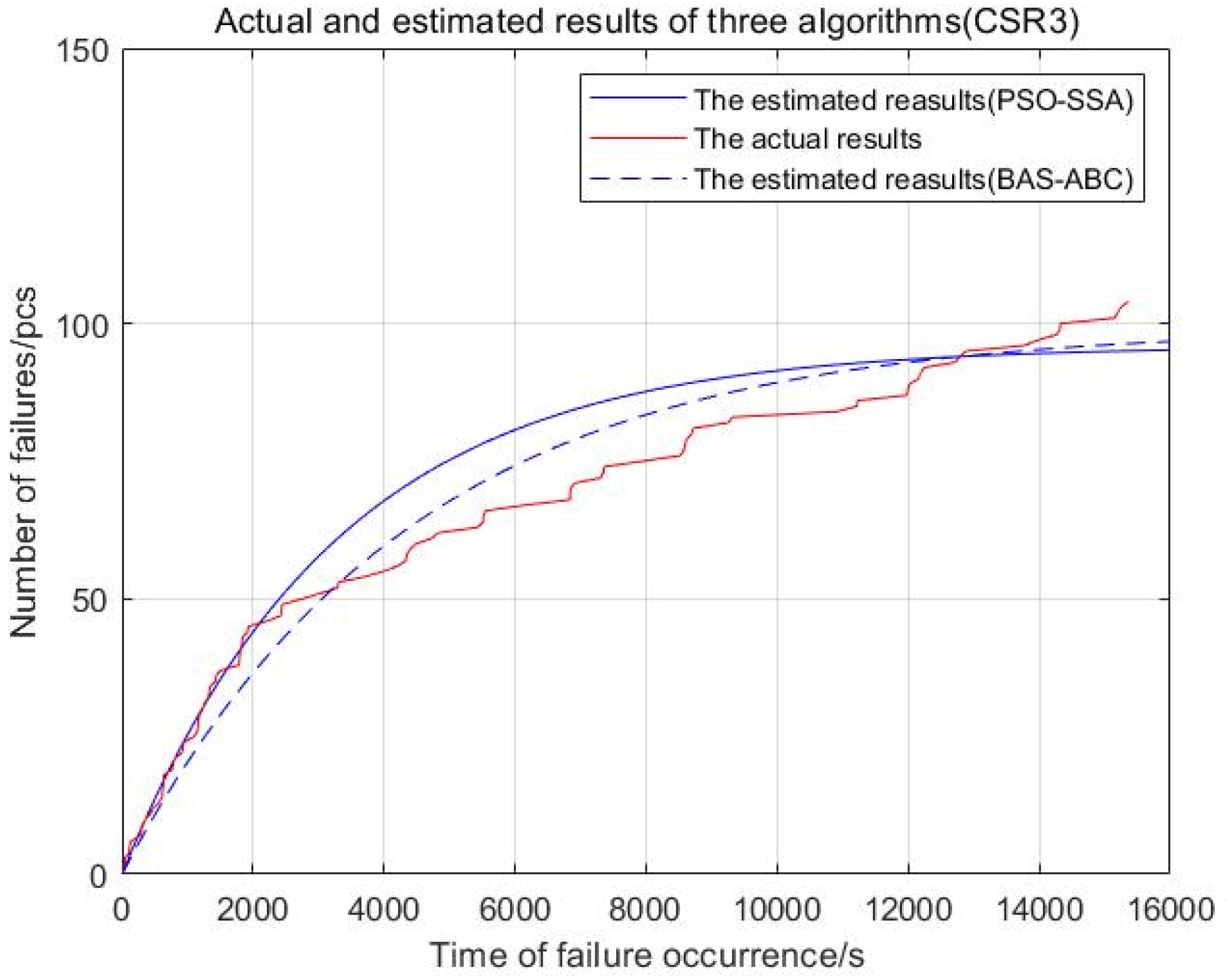
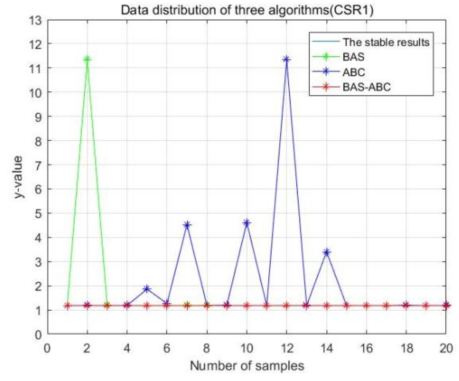
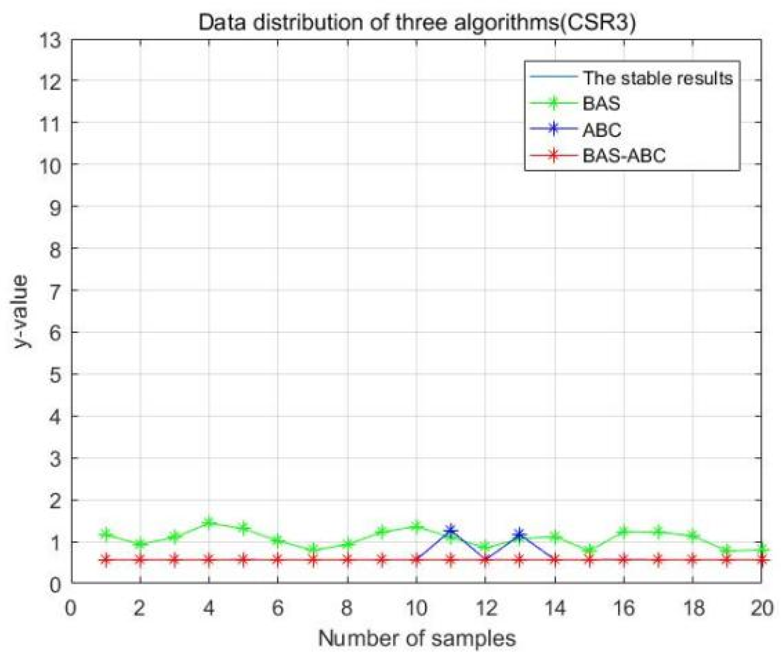
In Section 3, the three algorithms are compared and analyzed in part A on the basis of using the control function. In Section 3.1.1, an intuitive comparison is made between the failed curves and the model results of different algorithms, and the result shows that the estimation and prediction of the model by the hybrid algorithm are closest to the actual results. Section 3.1.2 Carries out statistical analysis on the optimal value, the worst value and the average value of the algorithm running 20 times, and finds that the accuracy of the hybrid algorithm is higher than that of the single algorithm. 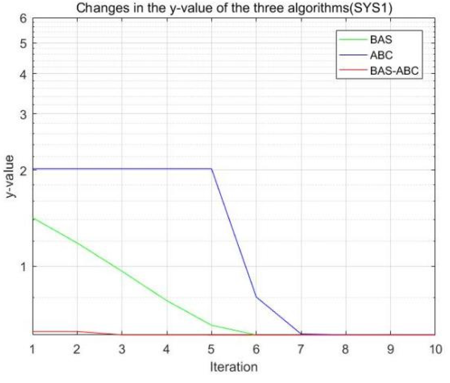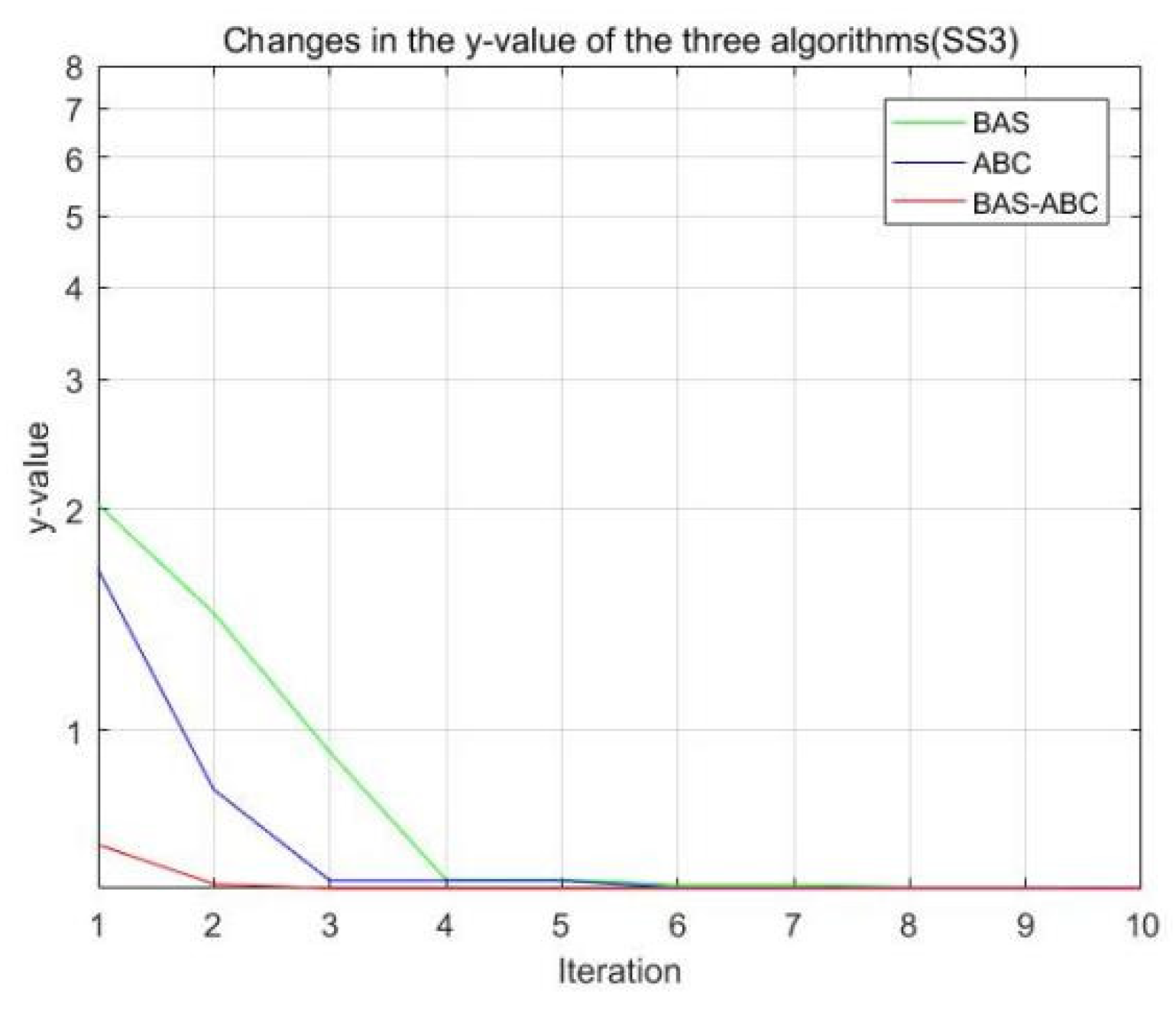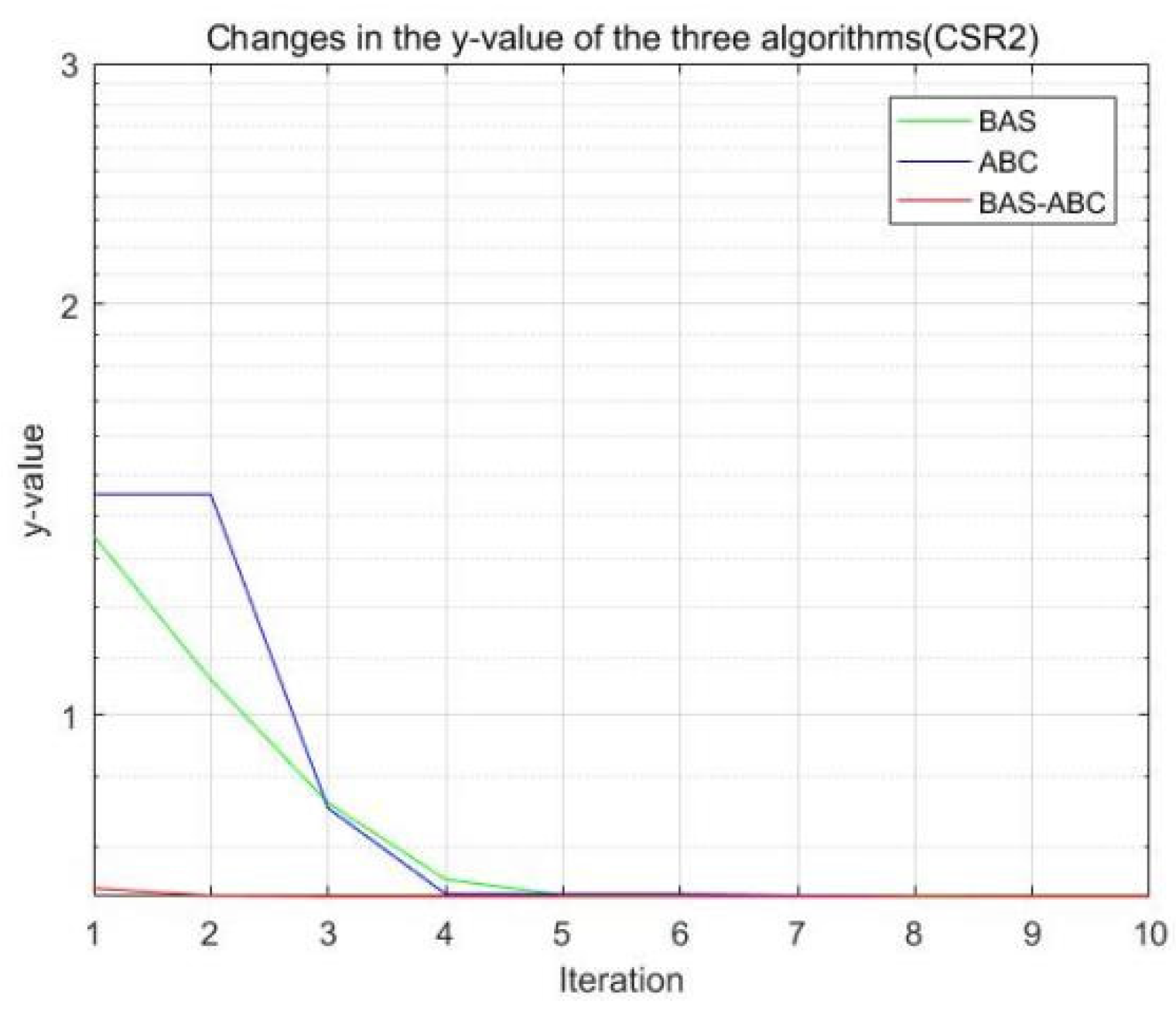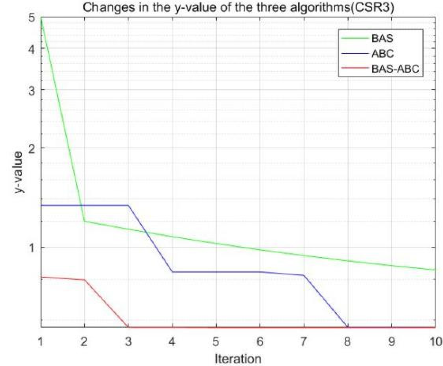In Section 3.1.3 and Section 3.1.4, the convergence speed and stability of the hybrid algorithm are better than that of the single algorithm. 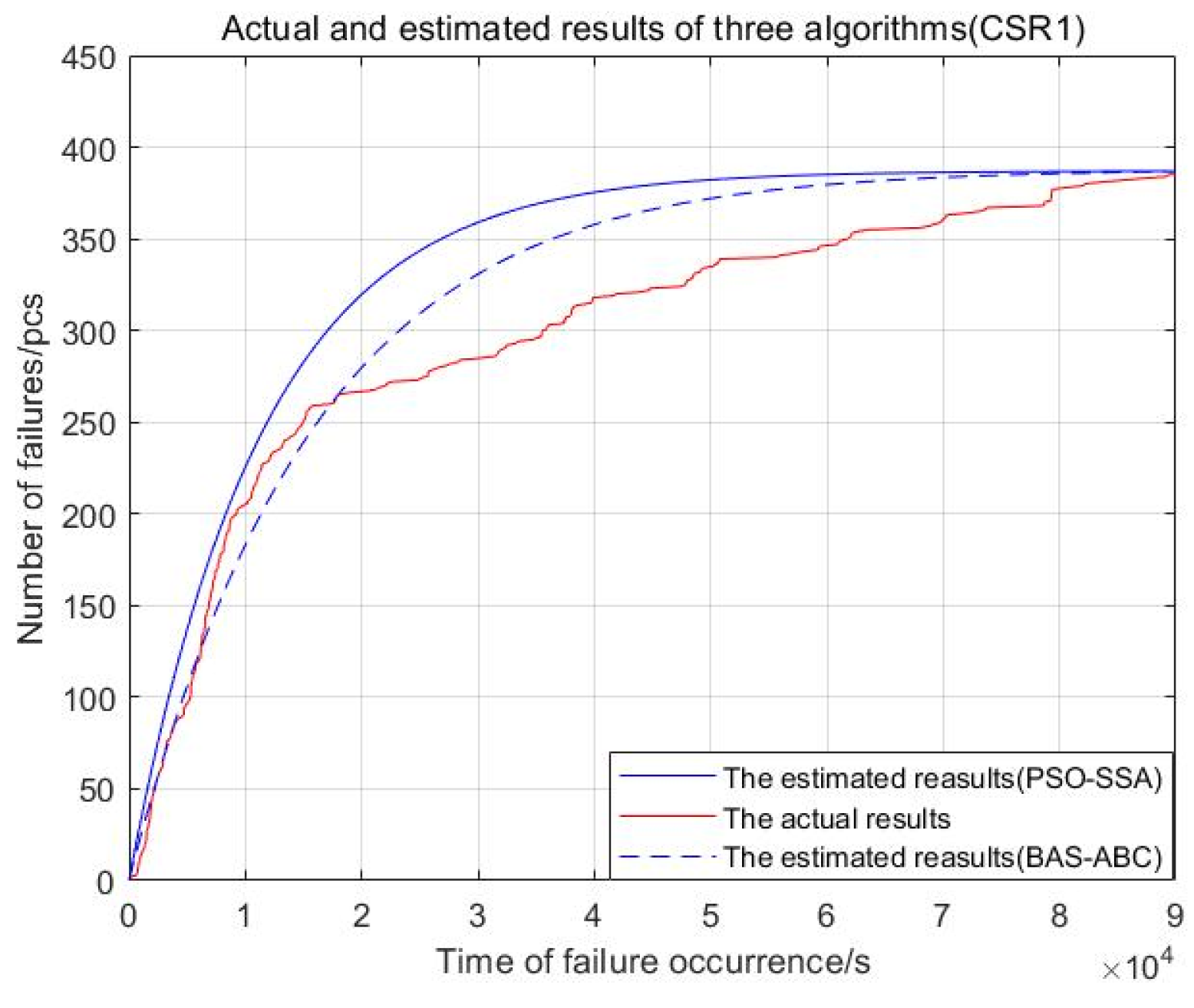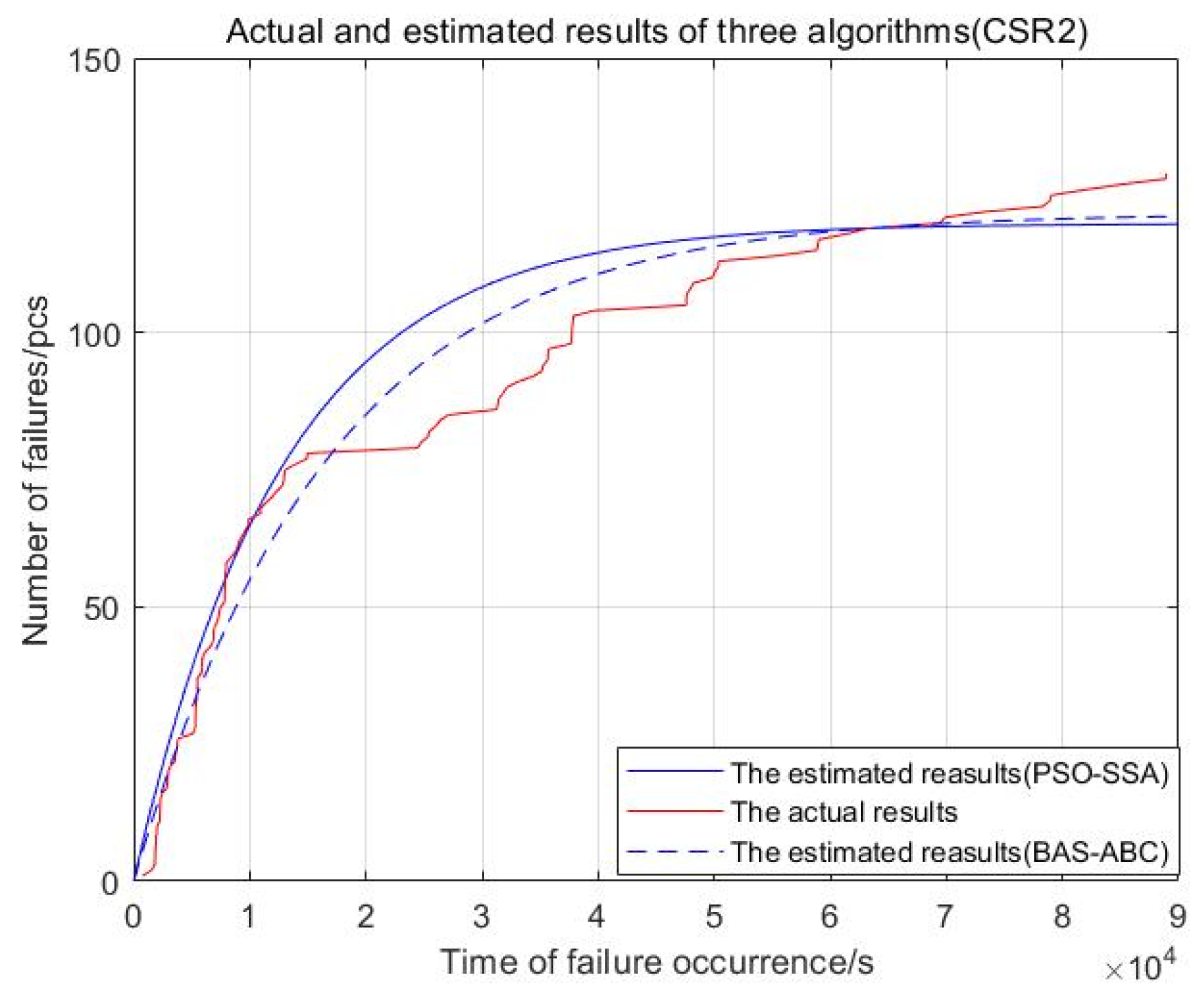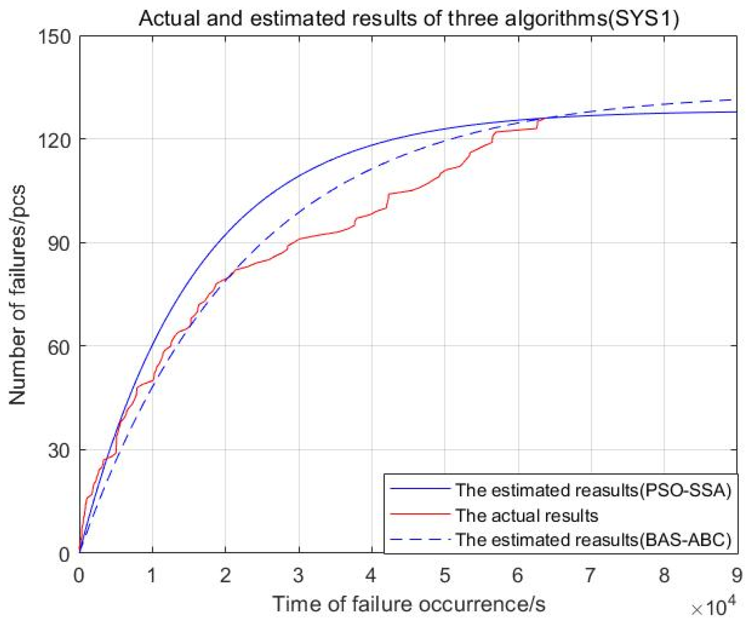In part B, the BAS-ABC hybrid algorithm proposed in this paper is compared with the PSO-SSA hybrid algorithm proposed in [3]. In Section 3.2.1, the actual failure curve is compared with the fitted curve of the two-hybrid algorithms, and it is found that the BAS-ABC is closer to the actual situation. In Section 3.2.2, the two-hybrid algorithms are run twenty times, respectively, and the optimal value, worst value and average value are statistically analyzed, and it is found that the accuracy rate of the BAS-ABC is higher than that of the PSO-SSA hybrid algorithm. 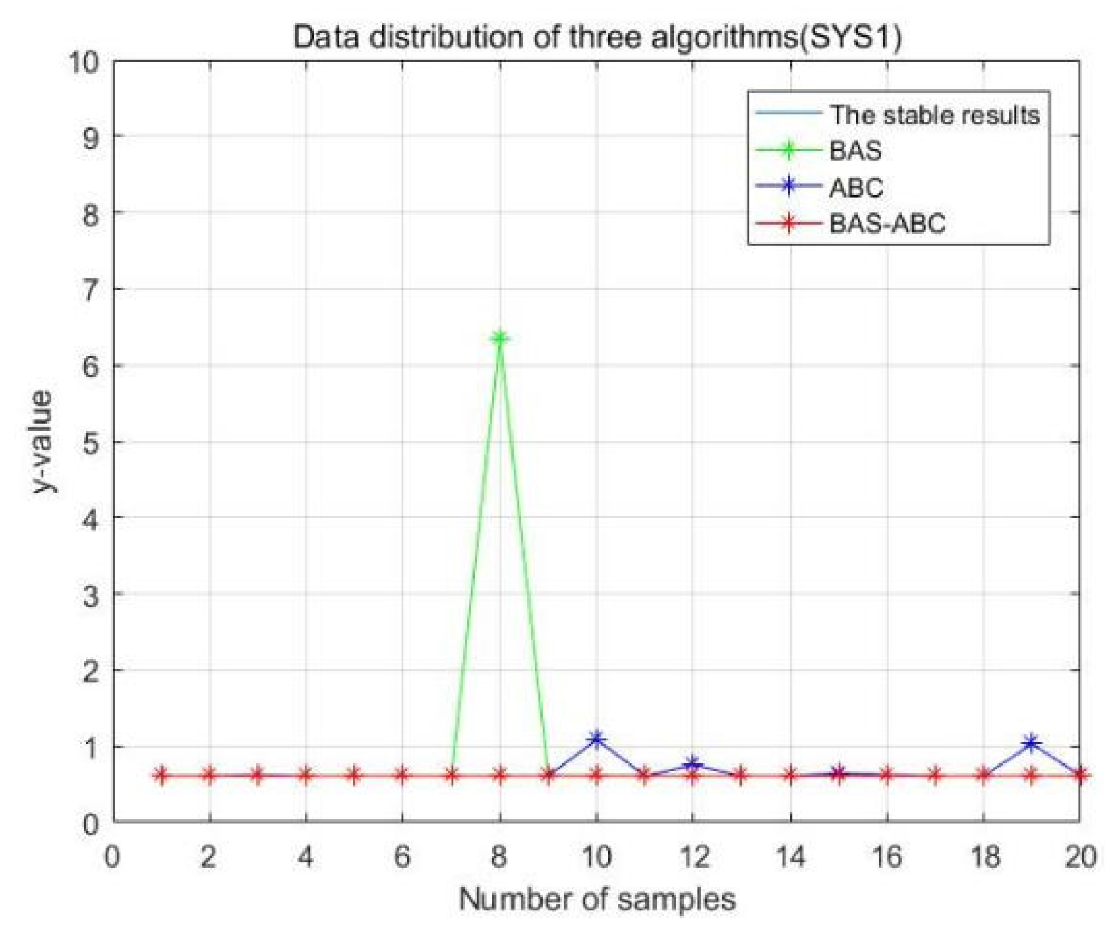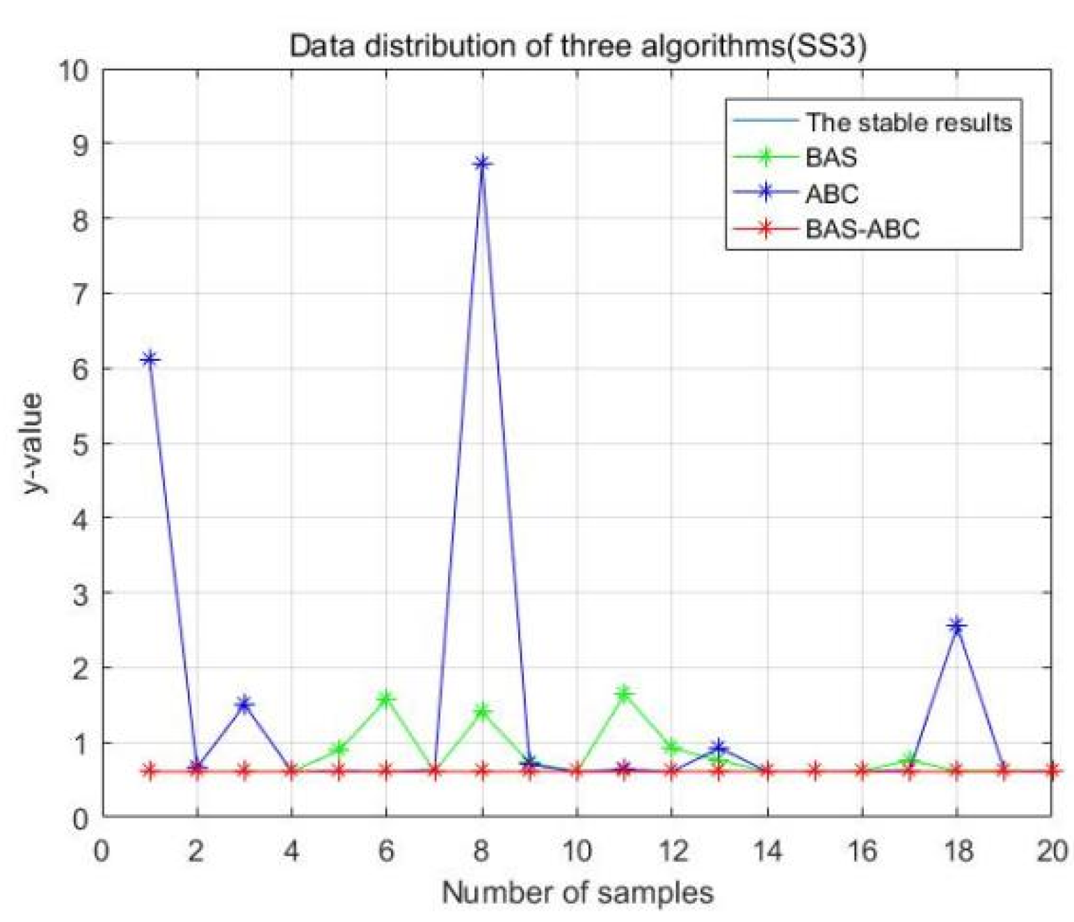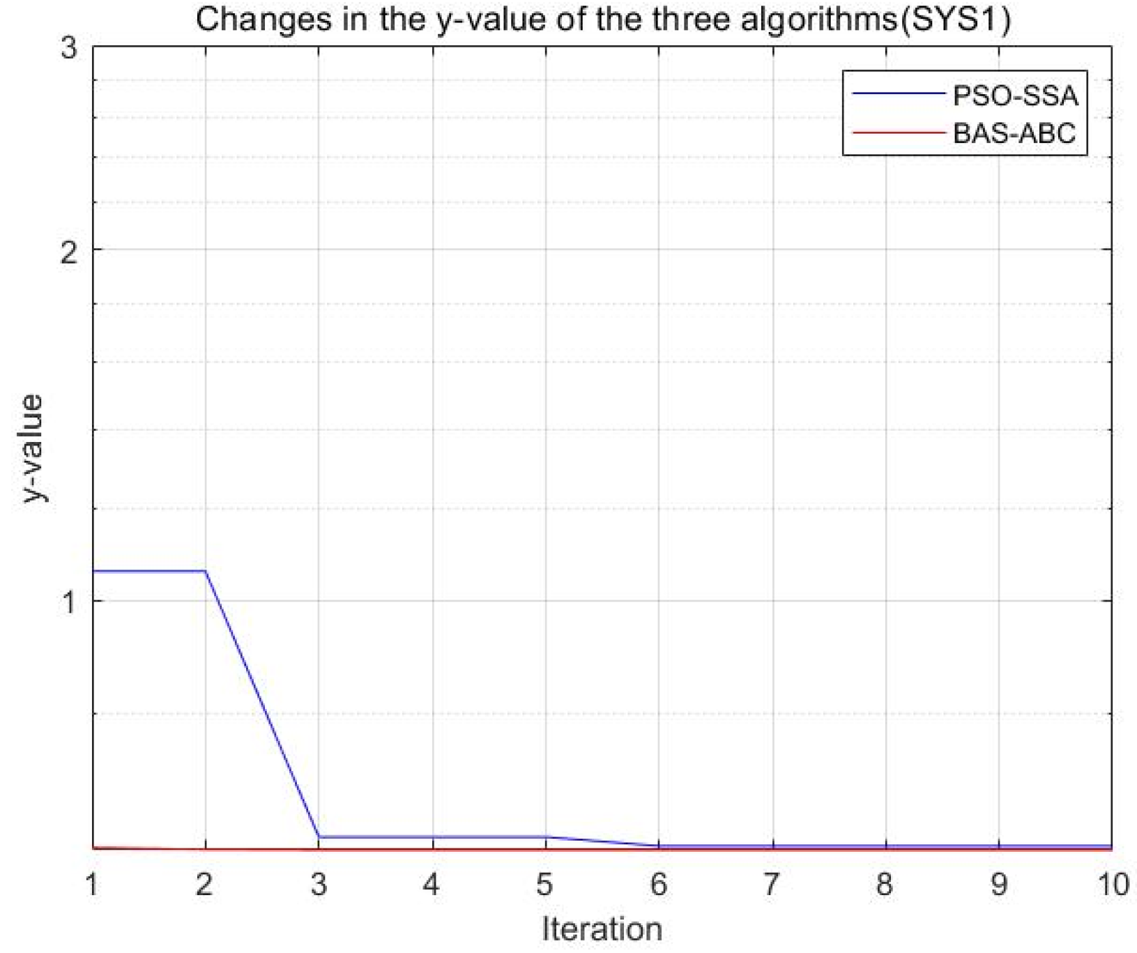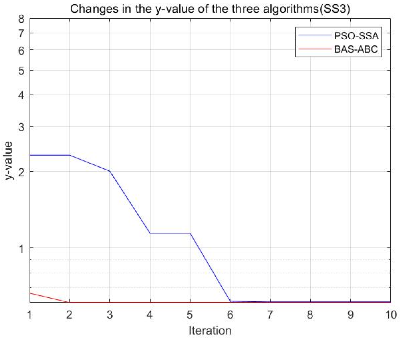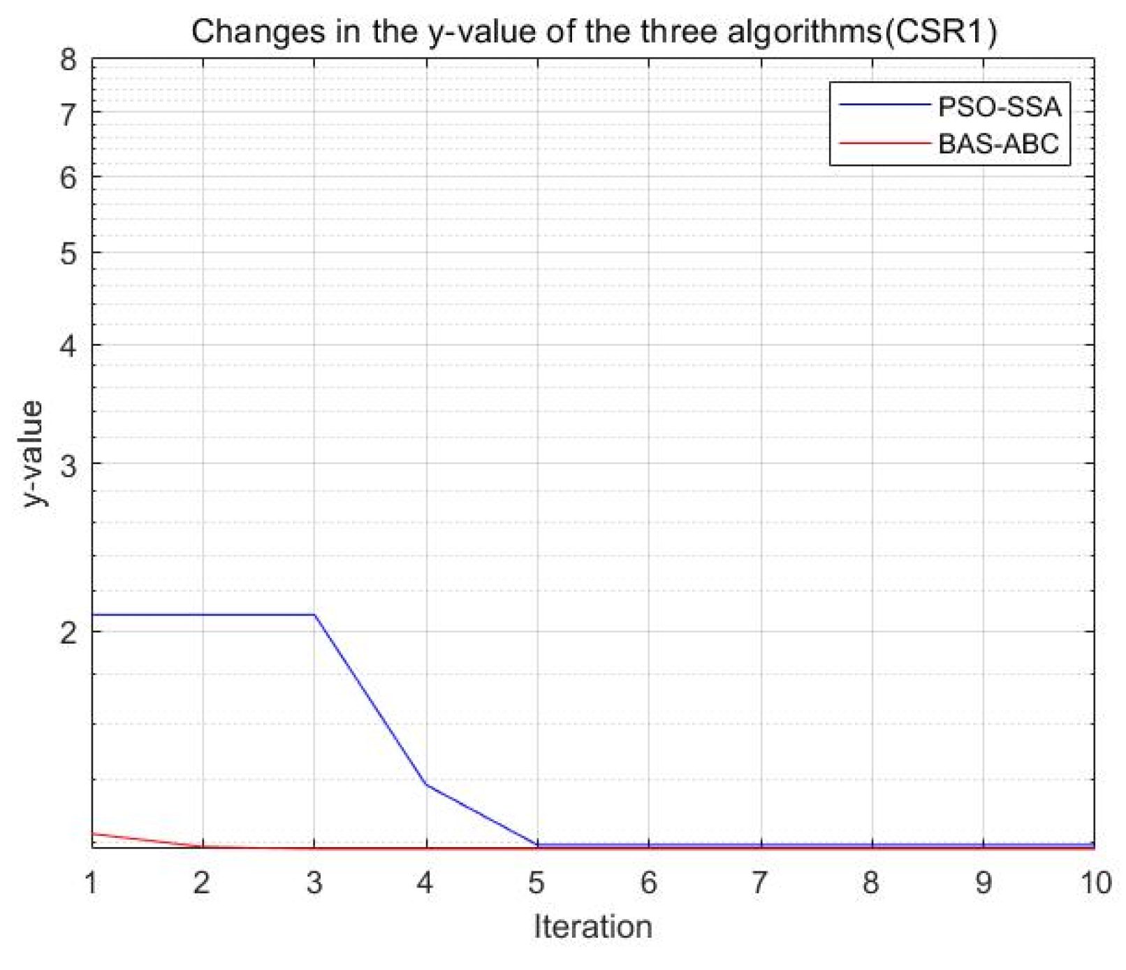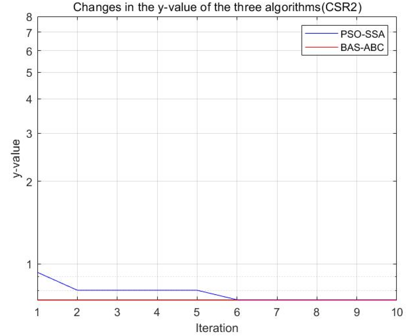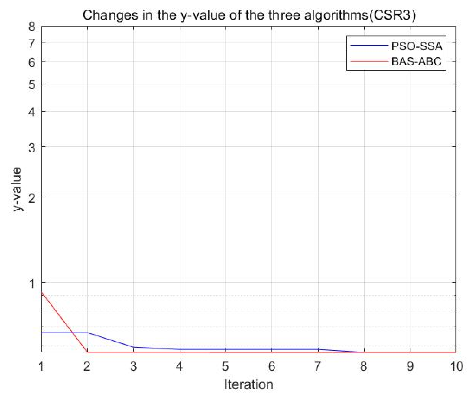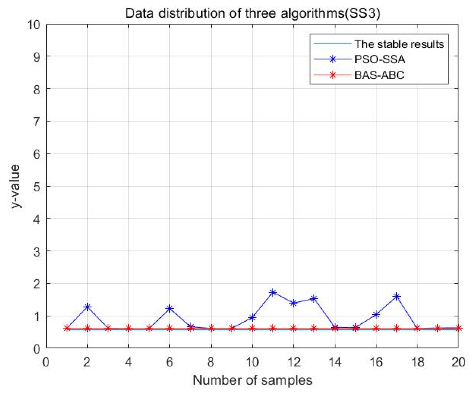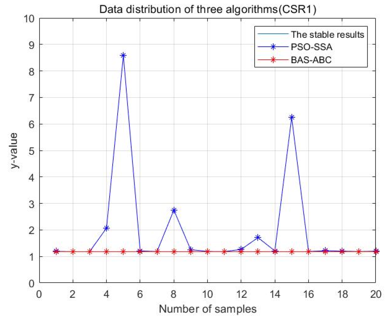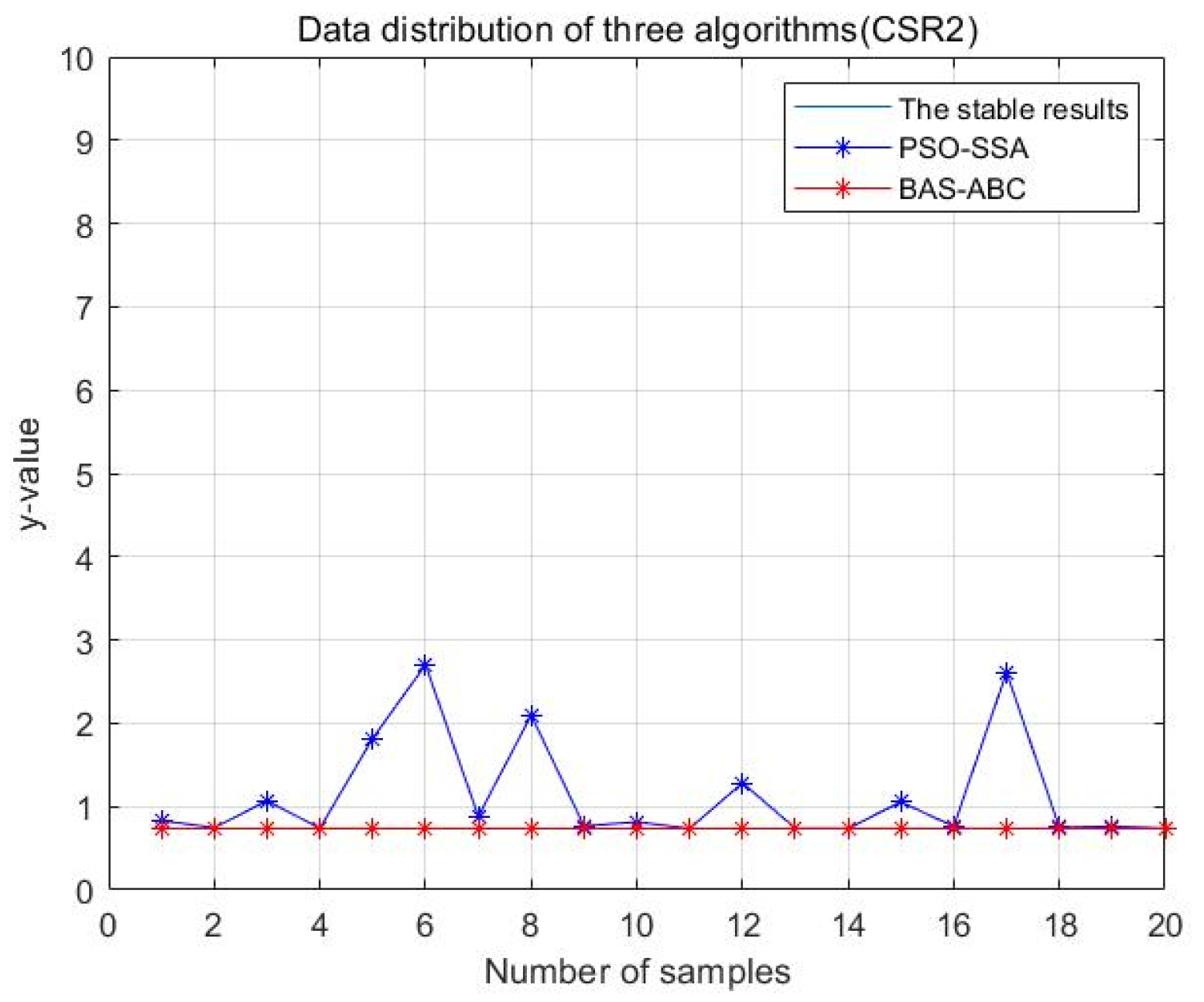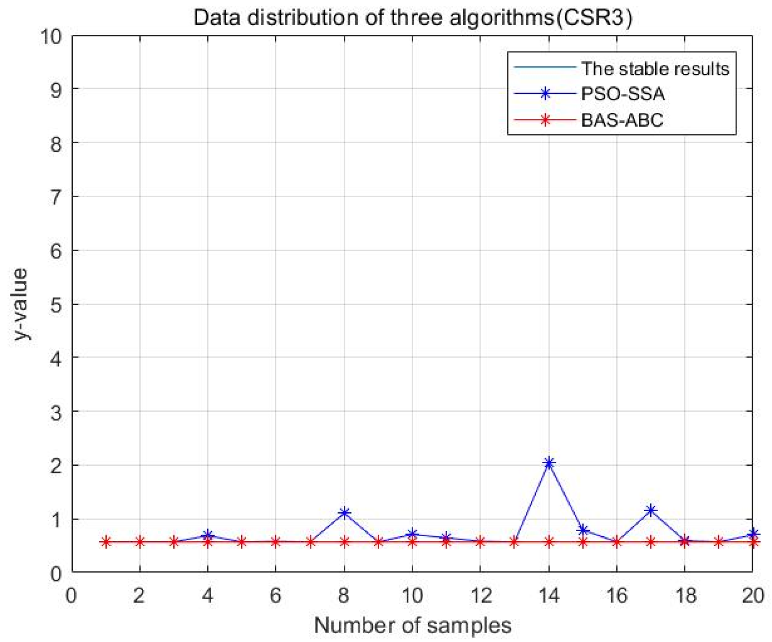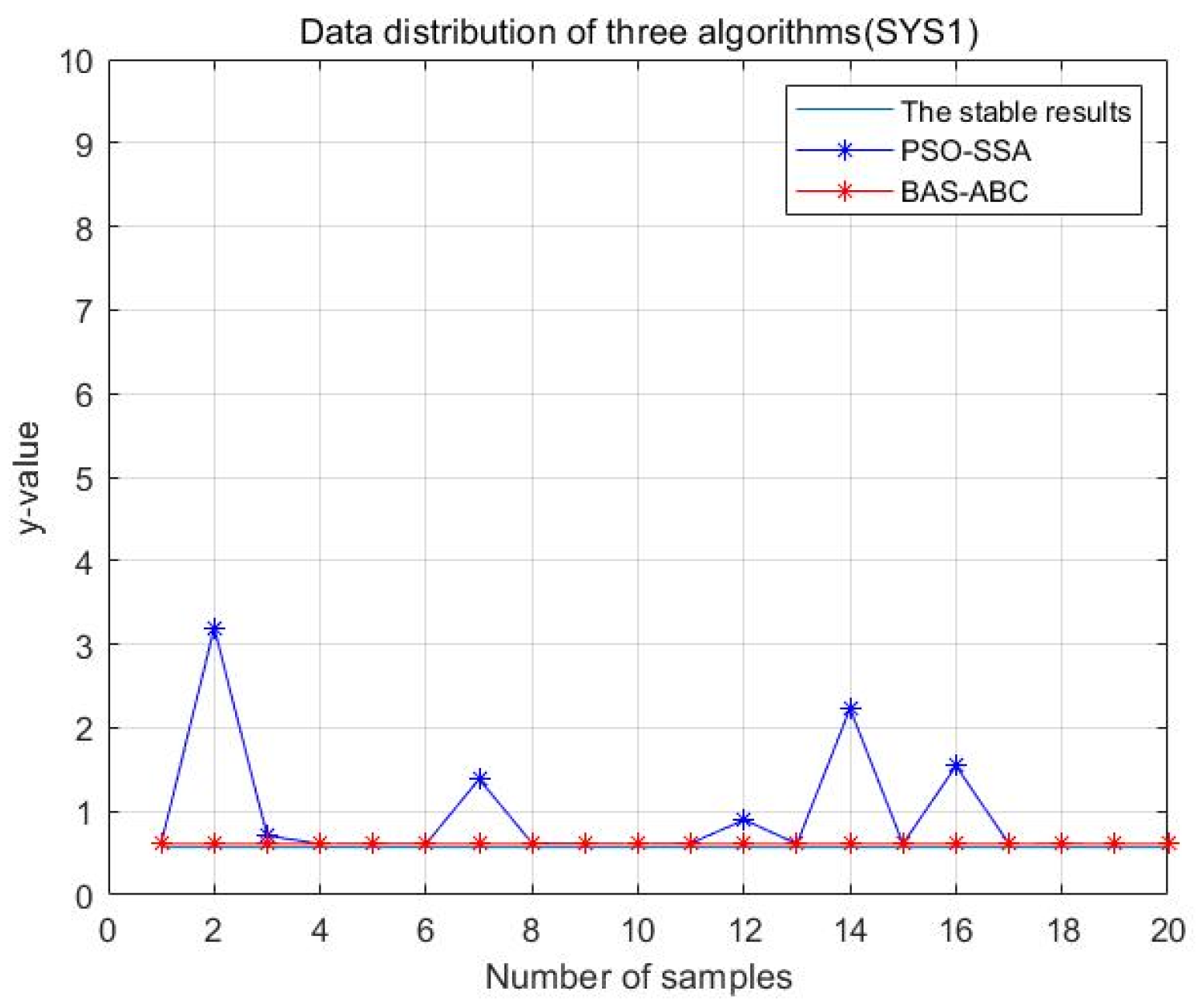In Section 3.2.3 and Section 3.2.4, the convergence speed and stability of the BAS-ABC are better than the PSO-SSA.

The algorithm is required to be able to quickly converge, the faster the better, and to improve the convergence speed that can be from two aspects including the initialization of the algorithm and the search process. The setting of the initial parameter value plays an important influence on the convergence of the algorithm, and a good initial parameter value can accelerate the convergence speed of the algorithm. As a result, using the BAS algorithm to get the optimal estimate of parameter $b$, and then using the ABC algorithm to start searching around it can speed up the convergence of the algorithm and improve the stability and accuracy of the results. The optimal value obtained by the BAS algorithm can avoid the randomness of honey source generation and realize the optimization of the search process of the artificial bee colony algorithm.

In fact, adding the BAS algorithm before the ABC algorithm can be regarded as optimizing the initial value of the ABC algorithm. All in all, the improved method of the algorithm convergence speed in this paper is to control the initialization of parameters in a better range, so as to ensure a smooth solution process.

5. Conclusions

In this paper, a hybrid algorithm based on BAS and ABC is proposed to estimate and predict the failure data of the G-O model by using a swarm intelligence algorithm.

According to the above experimental results, it can be found that the BAS-ABC algorithm proposed in this paper can predict parameters of the software reliability model more accurately and improve the prediction accuracy of software failure time. Compared with single BAS and ABC algorithms, the BAS-ABC algorithm can converge faster and its stability is greatly improved, which enables the algorithm to converge to the optimal value quickly, and the results obtained are more stable. In addition, comparing the BAS and ABC hybrid algorithm proposed in this paper with the PSO and SSA hybrid algorithm proposed in the literature [3], it can be found that the BAS-ABC hybrid algorithm has a faster convergence rate, and the obtained results have higher stability and accuracy. Furthermore, the hybrid BAS and ABC are faster in running time than the single ABC and BAS.

This paper selects the classic G-O model to estimate and predict. If the parameters of other software reliability models can be treated in the same way, the BAS-ABC hybrid algorithm proposed in this paper can achieve the same performance. In future research, a variety of models can be used for research, and the convergence of the algorithm can be judged in advance. When the algorithm is no longer convergent, the iterative search can be jumped out to improve the efficiency of the algorithm.

References

1. Ogîgău-Neamțiu, F.; Moga, H. A Cyber Threat Model of a Nation Cyber Infrastructure Based on Goel-Okumoto Port Approach. Land Forces Acad. Rev. 2018, 23, 75–87. [Google Scholar] [CrossRef] [Green Version]
2. Abuta, E.; Tian, J. Reliability over consecutive releases of a semiconductor Optical Endpoint Detection software system developed in a small company. J. Syst. Softw. 2018, 137, 355–365. [Google Scholar] [CrossRef]
3. Liu, Y.; Zhen, L.; Wang, D.S.; Hong, M.; Wang, Z.B. Software Defects Prediction Based on Hybrid Particle Swarm Optimization and Sparrow Search Algorithm. IEEE Access 2021, 9, 60865–60879. [Google Scholar]
4. Alaa, F.S.; Abdel-Raouf, A. Estimating the Parameters of Software Reliability Growth Models Using the Grey Wolf Optimization Algorithm. Int. J. Adv. Comput. Sci. Appl. 2016, 7, 499–505. [Google Scholar]
5. Choudhary, A.; Baghel, A.S. An efficient parameter estimation of software reliability growth models using gravitational search algorithm. Int. J. Syst. Assur. Eng. Manag. 2017, 8, 79–88. [Google Scholar] [CrossRef]
6. Kapil Sharma, S.; Bala, M. An ecological space based hybrid swarm-evolutionary algorithm for software reliability model parameter estimation. Int. J. Syst. Assur. Eng. Manag. 2020, 11, 77–92. [Google Scholar]
7. Zhu, M.; Pham, H. A software reliability model with time-dependent fault detection and fault removal. Vietnam. J. Comput. Sci. 2016, 3, 71–79. [Google Scholar] [CrossRef] [Green Version]
8. Lohmor, S.; Sagar, B.B. Estimating the parameters of software reliability growth models using hybrid DEO-ANN algorithm. Int. J. Enterp. Netw. Manag. 2017, 8, 247–269. [Google Scholar] [CrossRef]
9. Jiang, X.; Li, S. BAS: Beetle Antennae Search Algorithm for Optimization Problems. Int. J. Robot. Control 2008, 1. Available online: https://arxiv.org/pdf/1710.10724.pdf (accessed on 1 March 2021).
10. Yu, J.; Hou, X.; Zhao, A.; Nie, J.; Wang, F. Multi-objective optimal scheduling of home energy management system based on improved Longhorn whisker algorithm. J. Electr. Power Syst. Autom. 2022, 34, 79–86. [Google Scholar] [CrossRef]
11. Wen, J.; Li, J.; Sheng, C.; Chen, W. Application simulation of improved Longhorn whisker algorithm in shearer adjustment high school. Comput. Simul. 2021, 38, 311–315. [Google Scholar]
12. Sun, J.; Li, J.; Wang, D.; Sun, Y.; Luo, Z. Sparse array optimization of improved bee colony algorithm based on genetic model. Intense Laser Part. Beams. 2021, 33, 123005. [Google Scholar]
13. Dai, S.; Yang, G.; Li, M.; Zhao, Z.; Yu, K. Improved interference waveform decision of discrete artificial bee colony algorithm. Electroopt. Control 2019, 58, 1800–1807. [Google Scholar]
14. Yu, M.; Liu, S.; Pu, D. Optimization design of emergency vehicle path based on evolutionary bee colony algorithm under the influence of information transmission. J. Univ. Shanghai Sci. Technol. 2021, 43, 83–92. [Google Scholar]
15. Zhang, K.; Li, A.; Song, B. Parameter estimation method of software reliability model based on PSO. Comput. Eng. Appl. 2008, 44, 47–49. [Google Scholar]
Figure 1. Implementation of the BAS-ABC algorithm.
Axioms 11 00305 g001
Figure 2. Interpretable code of the algorithm architecture.
Axioms 11 00305 g002
Figure 3. Actual and estimated time of failure occurrence of three algorithms (SYS1).
Axioms 11 00305 g003
Figure 4. Actual and estimated time of failure occurrence of three algorithms (SS3).
Axioms 11 00305 g004
Figure 5. Actual and estimated time of failure occurrence of three algorithms (CSR1).
Axioms 11 00305 g005
Figure 6. Actual and estimated time of failure occurrence of three algorithms (CSR2).
Axioms 11 00305 g006
Figure 7. Actual and estimated time of failure occurrence of three algorithms (CSR3).
Axioms 11 00305 g007
Figure 8. Changes in the y value of the three algorithms (SYS1).
Axioms 11 00305 g008
Figure 9. Changes in the y value of the three algorithms (SS3).
Axioms 11 00305 g009
Figure 10. Changes in the y value of the three algorithms (CSR1).
Axioms 11 00305 g010
Figure 11. Changes in the y value of the three algorithms (CSR2).
Axioms 11 00305 g011
Figure 12. Changes in the y value of the three algorithms (CSR3).
Axioms 11 00305 g012
Figure 13. Data distribution-20 of three algorithms (SYS1).
Axioms 11 00305 g013
Figure 14. Data distribution-20 of three algorithms (SS3).
Axioms 11 00305 g014
Figure 15. Data distribution-20 of three algorithms (CSR1).
Axioms 11 00305 g015
Figure 16. Data distribution-20 of three algorithms (CSR2).
Axioms 11 00305 g016
Figure 17. Data distribution-20 of three algorithms (CSR3).
Axioms 11 00305 g017
Figure 18. Actual and estimated results of two algorithms (SYS1).
Axioms 11 00305 g018
Figure 19. Actual and estimated results of two algorithms (SS3).
Axioms 11 00305 g019
Figure 20. Actual and estimated results of two algorithms (CSR1).
Axioms 11 00305 g020
Figure 21. Actual and estimated results of two algorithms (CSR2).
Axioms 11 00305 g021
Figure 22. Actual and estimated results of two algorithms (CSR3).
Axioms 11 00305 g022
Figure 23. Changes in the y value of the two algorithms (SYS1).
Axioms 11 00305 g023
Figure 24. Changes in the y value of the two algorithms (SS3).
Axioms 11 00305 g024
Figure 25. Changes in the y value of the two algorithms (CSR1).
Axioms 11 00305 g025
Figure 26. Changes in the y value of the two algorithms (CSR2).
Axioms 11 00305 g026
Figure 27. Changes in the y value of the two algorithms (CSR3).
Axioms 11 00305 g027
Figure 28. Data distribution—20 of two hybrid algorithms (SYS1).
Axioms 11 00305 g028
Figure 29. Data distribution—20 of two hybrid algorithms (SS3).
Axioms 11 00305 g029
Figure 30. Data distribution—20 of two hybrid algorithms (CSR1).
Axioms 11 00305 g030
Figure 31. Data distribution—20 of two hybrid algorithms (CSR2).
Axioms 11 00305 g031
Figure 32. Data distribution—20 of two hybrid algorithms (CSR3).
Axioms 11 00305 g032