Article

Multitask Learning Based on Least Squares Support Vector Regression for Stock Forecast

1
School of Automation, Xi’an University of Posts and Telecommunications, Xi’an 710121, China
2
Xi’an Key Laboratory of Advanced Control and Intelligent Process, Xi’an 710121, China
*
Authors to whom correspondence should be addressed.
Axioms 2022, 11(6), 292; https://doi.org/10.3390/axioms11060292
Submission received: 30 May 2022 / Revised: 9 June 2022 / Accepted: 10 June 2022 / Published: 15 June 2022
(This article belongs to the Special Issue Soft Computing with Applications to Decision Making and Data Mining)

Abstract

:
Various factors make stock market forecasting difficult and arduous. Single-task learning models fail to achieve good results because they ignore the correlation between multiple related tasks. Multitask learning methods can capture the cross-correlation among subtasks and achieve a satisfactory learning effect by training all tasks simultaneously. With this motivation, we assume that the related tasks are close enough to share a common model whereas having their own independent models. Based on this hypothesis, we propose a multitask learning least squares support vector regression (MTL-LS-SVR) algorithm, and an extension, EMTL-LS-SVR. Theoretical analysis shows that these models can be converted to linear systems. A Krylov-Cholesky algorithm is introduced to determine the optimal solutions of the models. We tested the proposed models by applying them to forecasts of the Chinese stock market index trend and the stock prices of five stated-owned banks. The experimental results demonstrate their validity.
MSC:
65E99; 68T01; 68U01; 91G80; 91B55

1. Introduction

The stock market is an indispensable part of the securities and financial industries. It reflects a country’s economic situation and development. However, the behavior of a stock market is affected by many factors, such as financial and economic policy, business development, and investor psychology [1]. Due to complex internal factors and the changing economic environment, forecasting the stock market is a challenge for researchers of financial data mining [2]. Traditional stock market forecasting methods include securities investment analysis, nonlinear dynamic methods, time series mining, and statistical modeling [3].
Securities investment analysis requires close attention to the international and domestic events along with keen market insight [4,5]. Considering the nonlinear character of the financial trading market, some nonlinear forecasting models have been established on the basis of nonlinear dynamical theory [6,7]. Chen et al. [8] studied a multifactor time series model for stock index forecasting, which achieved a low root mean square error. Some statistical methods require strong modeling and statistical capabilities, which is difficult for general investors [9].
Many machine learning and deep learning methods are used to forecast the stock market and analyze stock prices. A high-performance stock trading architecture which integrates neural networks and trees is developed by Chalvatzis et al. [10], which is presented to enhance profitability during the investment. Zhang et al. [11] presented a model based on support vector regression (SVR) and a modified firefly algorithm to forecast stock prices. A back propagation (BP) neural network was extended to predict the stock market [12,13], but it fell easily into a local optimal solution. Song et al. [14] developed a deep learning model to forecast stock price fluctuation, which included hundreds of input-features. To explore the impact of historical events, a stacked long short term memory network was adopted to predict stock market behavior [15]. However, their work inevitably built many irregular hidden network layers. Li et al. [16] proposed MISA-K-ELM, integrating mutual information-based sentimental analysis with kernel extreme learning machine to forecast stock prices. Dash et al. [17] proposed a self-evolving recurrent neuro-fuzzy inference system to predict irregular financial time series data. Text mining was applied to analyze financial articles and investor sentiment to predict daily stock market behavior [18,19]. Mohanty et al. [20] proposed a hybrid model combined with auto encoder (AE) and kernel extreme learning machine (KELM), and the prime advantage of the proposed technique over the conventional SAE is robust prediction of different financial markets with reduction in error. These methods performed well at forecasting stock market trends, but they ignored the essential relatedness among stock data.
As an important and ongoing issue in machine learning, multitask learning has attracted significant attention in many fields, such as supervised learning, semi-supervised learning, reinforcement learning, and multiview learning [21]. According to the concept of multitask learning, there is shared useful information among multiple related tasks, hence the learning effect of tasks can be well enhanced. When there are intrinsic relations among subtasks, the learning effect of all tasks can be greatly improved by learning them simultaneously. Gao [22] adopted clustered multitask support vector regression (MT-SVR) to perform age estimation based on facial images, which required the solution of large-scale quadratic programming problems. Li et al. [23] proposed multitask proximal support vector machine (MTPSVR), which incurred a lower computational cost than MT-SVR. Xu et al. [24] applied multitask least squares support vector machine (MTLS-SVM) to analyze three components of broomcorn samples. Nevertheless, MTLS-SVM confused the common bias and the bias in the subtask decision function, and could not flexibly select an appropriate kernel function according to different information.
In this paper, we develop a multitask learning assumption such that each subtask model can be obtained by solving a common model and an independent model. Then multitask learning least squares support vector regression (MTL-LS-SVR) is proposed under the assumption that the same kernel functions are employed in the common model and independent models. In addition, we propose an extension of MTL-LS-SVR, EMTL-LS-SVR, which cannot only consider the internal cross-correlation among subtasks but can select different kernel functions for the common model and independent models. These features can improve the prediction performance more efficiently than other training algorithms. Next, we present the Krylov-Cholesky algorithm to solve the proposed models, which greatly improves the training speed. Finally, the proposed models are applied to forecast the Chinese stock market index trend and the stock price movements of five state-owned banks.

2. Least Squares Support Vector Regression

SVR attempts to minimize the generalization error bound under the structural risk minimization principle. It is based on a generalized linear regression function f x = φ x T ω * + b * in a high-dimensional feature space [25]. The inequality constraints in SVR are transformed to equality constraints by least squares, which greatly improves the efficiency of training LS-SVR [26]. Given a set of input samples, LS-SVR trains the generalized linear regression function to complete the regression prediction by a nonlinear mapping. The decision function of LS-SVR can be obtained by solving the following optimization problem
min J ω , b , ξ = 1 2 ω 2 + C 2 i = 1 n ξ i 2 s . t . y i = ω T φ x i + b + ξ i , i = 1 , 2 , , n
where J denotes an objective function, the symbol T represents the transpose of a certain matrix or vector, and φ is a nonlinear mapping from the original input space to the feature space. C is a penalty coefficient, and ξ = ξ 1 , ξ 2 , , ξ n T is a slack vector to reflect whether the samples can be located in the ε -tube. ω , b is the generalized weight vector to be solved. x and y are respective sample attributes and tags.
The Lagrange function method is used to transform the quadratic programming problem (1) to a linear system
Q I n I n T 0 α b = Y 0
where I n = 1 , 1 , , 1 T is an n × 1 vector of ones. α and b are the Lagrange multiplier vector and threshold. Q = Ω + E n C n × n is a positive definite matrix, and E n is an n-dimensional identity matrix. Ω is an n × n matrix with elements ω i , j = φ x i T φ x j = K x i , x j . φ is a nonlinear mapping from the original input space to the feature space, and K , is the corresponding kernel function. Solving the linear system (2) gives us the following regression function
f x = φ x T ω * + b * = i = 1 n α i * K x i , x j + b * .

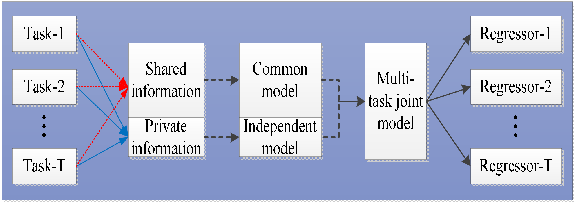
3. Extension of Multitask Learning Least Squares Support Vector Regression

Suppose we have T T > 1 learning tasks that are distinct but have good internal cross-correlation. For every task, there are m t training data x t i , y t i i = 1 m t , where x t i d and y t i . Hence, we have m = t = 1 T m t training data.
Multitask learning aims to train subtasks at the same time and uses the effective information among related tasks to improve the generalization ability of the regression model. Since multiple tasks are related and different, there is shared information among all tasks and private information belonging to the subtasks themselves. We assume that all tasks share a common model ρ 0 and each subtask has an independent submodel η t ,   t = 1 , 2 , , T . The regression function corresponding to the t t h subtask can be expressed as ρ t = ρ 0 + η t . To clearly illustrate multitask learning, Figure 1 shows a block diagram of our proposed models.
We first establish MTL-LS-SVR, and an extension, EMTL-LS-SVR. Next, we present a Krylov-Cholesky algorithm to solve large-scale multitask learning problems.

3.1. MTL-LS-SVR

In the multitask learning model MTL-LS-SVR, the subtask model is represented as
ρ t = ρ 0 + η t = ω 0 , φ + υ t , φ + b 0 + b t
where ω 0 and φ are, respectively, the normal vector and nonlinear mapping function for the common model ρ 0 , and υ t and φ are those of the independent model η t . b 0 is the bias of the common hyperplane, and b t is the threshold difference between the hyperplane corresponding to the t t h subtask and the common hyperplane. υ t tends to zero if the subtasks are closely related, and ω 0 tends to zero otherwise.
The MTL-LS-SVR model can be determined by solving the following optimization problem
min   J = 1 2 ω 0 2 + λ 2 T t = 1 T υ t 2 + b t 2 + C 2 t = 1 T ξ t 2 s . t .   y t = A t ω 0 + υ t + b 0 + b t I m t + ξ t ,   t = 1 , 2 , , T
where ξ t = ξ t 1 , ξ t 2 , , ξ t m t T represents the slack variable vectors for the t t h subtask. C is a positive regularization coefficient. The dataset of the t t h subtask is mapped to the feature space by the nonlinear mapping ϕ , which can be denoted by A t = φ x t 1 T , φ x t 2 T , , φ x t m t T T . I m t m t × 1 , is a column vector of ones. For all the learning tasks, the task-coupling parameter λ balances the trade-off relationship between the shared information and the private information among all tasks. In particular, the greater the value of λ , the stronger the degree of association among subtasks; otherwise, the degree of association is weaker. It can be seen that subtasks are trained at the same time because they share some internal information.
The Lagrange function of the quadratic programming problem (5) is as follows:
L = 1 2 ω 0 2 + λ 2 T t = 1 T υ t 2 + b t 2 + C 2 t = 1 T ξ t 2 t = 1 T α t T A t ω 0 + υ t + b 0 + b t I m t + ξ t y t
where α t = α t 1 , α t 2 , , α t m t T is a nonnegative Lagrange multiplier vector. According to the Karush–Kuhn–Tucker KKT condition, we derive the linear system
Q m × m 1 H m × 1 H m × 1 T 0 α m × 1 b 0 = Y m × 1 0
where Q 1 = A A T + T λ Ω 1 + E m C is an m × m positive definite matrix, and Ω 1 is a block-wise diagonal matrix noted as Ω 1 = b l k d i a g A t A t T + I m t I m t T m × m , t = 1 , 2 , , T . E m is an m-dimensional identity matrix. H is a column vector of ones, b 0 is the threshold of the common hyperplane, and α m × 1 = α 1 T , α 2 T , , α T T T . Solving the linear system (7) gives us the Lagrange multiplier vector α , bias item b 0 , and regression parameters corresponding to the common hyperplane and private information. Therefore, the decision function of MTL-LS-SVR can be obtained as
f t x = φ x ω 0 * + υ t * + b 0 * + b t * = φ x A T α * + T λ A t T α t * + T λ i = 1 m t I m t T α t i * + b 0 * = t = 1 T i = 1 m t α t i * K x t i , x + T λ i = 1 m t α t i * K x t i , x + T λ i = 1 m t I m t T α t i * + b 0 * .

3.2. EMTL-LS-SVR

In the MTL-LS-SVR model, to select the same kernel functions for the common model and independent models cannot effectively distinguish their essential differences. Therefore, we propose an extension of MTL-LS-SVR, EMTL-LS-SVR. The regression function corresponding to the t t h subtask can be represented as
ρ t = ρ 0 + η t = ω 0 , φ + υ t , ϕ + b 0 + b t
where ρ t represents the joint model of the t t h subtask, ρ 0 and η t respectively denote the common model and private model. ω 0 and φ are, respectively, the normal vector and nonlinear mapping function for the common model, and υ t and ϕ are those of the independent model η t . It is obvious that φ and ϕ are different nonlinear mappings, hence different kernel functions are applied to process the shared information and private information.
According to the above analysis, the optimization problem of EMTL-LS-SVR can be obtained as
min   J = 1 2 ω 0 2 + λ 2 T t = 1 T υ t 2 + b t 2 + C 2 t = 1 T ξ t 2 s . t .   y t = A t ω 0 + A ˜ t υ t + b 0 + b t I m t + ξ t ,   t = 1 , 2 , , T
where the dataset of the t t h subtask is mapped to the feature space by the nonlinear mapping ϕ that can be noted as A ˜ t = ϕ x t 1 T , ϕ x t 2 T , , ϕ x t m t T T . λ , T , ξ t , A t , φ , I m t , b 0 , and b t have the same meanings as in the quadratic programming problem (5).
The corresponding Lagrange function of the quadratic programming problem (10) is
L = 1 2 ω 0 2 + λ 2 T t = 1 T υ t 2 + b t 2 + C 2 t = 1 T ξ t 2 t = 1 T α t T A t ω 0 + A ˜ t υ t + b 0 + b t I m t + ξ t y t
where α t is the nonnegative Lagrange multiplier vector denoted as α t = α t 1 , α t 2 , , α t m t T . Setting the gradient of Lagrange function (11) with respect to ω 0 , υ t , b 0 , b t , ξ t and α t to zero, we obtain the following equations:
L ω 0 = 0 ω 0 = t = 1 T A t T α t = A T α , L υ t = 0 υ t = T λ A ˜ t T α t , L b 0 = 0 t = 1 T I m t T α t = 0 , L b t = 0 b t = T λ I m t T α t , L ξ t = 0 ξ t = 1 C α t , L α t = 0 A t ω 0 + A ˜ t υ t + b 0 + b t I m t + ξ t = y t .
Then, refer to Equation (12), we can obtain the linear system
Q m × m 2 H m × 1 H m × 1 T 0 α m × 1 b 0 = Y m × 1 0
where Q 2 = A A T + T λ Ω 2 + E m C is a positive definite matrix, and Ω ( 2 ) is a block-wise diagonal matrix noted as Ω ( 2 ) = b l k d i a g ( A ˜ t A ˜ t T + I m t I m t T ) m × m , t = 1 , 2 , , T . E m , H , b 0 , and α m × 1 have the same meanings as for the linear system (7). By solving the linear system (13), we obtain the Lagrange multiplier vector α m × 1 and threshold b 0 , and the regression parameters corresponding to the common model and independent sub-models can also be determined. Therefore, the decision function of EMTL-LS-SVR can be obtained as
f t ( x ) = φ x ω 0 * + ϕ x υ t * + b 0 * + b t * = φ x A T α * + T λ ϕ x A ˜ t T α t * + b 0 * + b t * = t = 1 T i = 1 m t α t i * K 0 x t i , x + T λ i = 1 m t α t i * K t x t i , x + T λ i = 1 m t I m t T α t i * + b 0 *
where K 0 , and K t , are the respective kernel functions in the common model and independent models. It is obvious that EMTL-LS-SVR is reduced to MTL-LS-SVR if and only if φ is equivalent to ϕ .

3.3. Krylov-Cholesky Algorithm

The linear systems (7) and (13) contain respective m + 1 equations, and are difficult to solve directly if the coefficient matrices are not positive definite. By using the Krylov methods [27], we can convert these linear systems to the form
Q m × m i 0 m × 1 0 m × 1 T s Q i 1 H b 0 + α m × 1 b 0 = Y m × 1 H T Q i 1 Y
where Q m × m i i = 1 , 2 are the respective positive definite matrices when solving MTL-LS-SVR and EMTL-LS-SVR, which we can denote as Q i = A A T + T λ Ω i + E m C , i = 1 , 2 . s = H T Q i 1 H is a positive number. Therefore, the linear system (13) is also positive definite. We will need to calculate the inverses of the large matrices Q i , which can be time-consuming. In fact, Q i is positive definite and symmetric, hence Q i 1 can be simplified by the Cholesky factorization method [28]. Hence, we develop a Krylov-Cholesky algorithm to solve the proposed models. To describe the model establishment process, Figure 2 shows the flowchart of the proposed multitask learning models.
The Krylov-Cholesky algorithm steps are listed as follows:
(1)
Convert the linear system (7) or (13) to the following form using Krylov methods:
Q m × m 0 m × 1 0 m × 1 T s Q 1 H b 0 + α m × 1 b 0 = Y m × 1 H T Q 1 Y
where s = H T Q 1 H is a positive number. Q m × m is a positive definite and symmetric matrix denoted as Q = A A T + T λ Ω + E m C , and Ω is an m × m block-wise diagonal matrix;
(2)
Apply the Cholesky factorization method to decompose Q into Q = L L T , and the elements l i j of the lower-triangular matrix L can be determined from Q ;
(3)
Calculate L 1 , and thus L T 1 = L 1 T , Q 1 = L 1 T L 1 ;
(4)
Solve R , τ from Q R = H and Q τ = Y , respectively, and record the corresponding solution R * and τ * ;
(5)
Calculate s = H T R * ;
(6)
Obtain the optimal solution: b 0 * = 1 s H T τ * and α * = τ * R * b 0 * .
According to the Krylov-Cholesky algorithm, we can obtain the optimal solutions of linear systems (7) and (13) by solving linear system (16). We can apply the Krylov methods to convert the original linear system to a new one with a sparser coefficient matrix. We use the Cholesky factorization method to decompose Q into the product of a lower-triangular matrix L and its upper-triangular conjugate transpose L T . Q 1 is optimized by solving the inverse of L . The optimal solutions of linear systems (7) and (13) can be determined by solving for b 0 and α , respectively.

4. Experiments

To verify the effectiveness of the proposed multitask learning models, we compared them to SVR, LS-SVR, MTPSVR [23], and MTLS-SVR [24]. Experiments were performed in MATLAB R2016a on a PC with an Intel Core i5-2500 CPU (3.30 GHz) and 8 GB of RAM. In our experiments, the radial basis function kernel K x i , x j = exp σ x i x j 2 is employed in MTL-LS-SVR and four comparative models. For EMTL-LS-SVR, we used kernel functions K 0 and K t in the common model and independent models, respectively, as referred (14). Three combinations were used:
1)
K 0 is a linear kernel and K t is a polynomial kernel.
2)
K 0 is a linear kernel and K t is a radial basis function kernel.
3)
K 0 is a polynomial kernel and K t is a radial basis function kernel.
For convenience, “L”, “P”, and “R”, respectively, represent linear kernel K x i , x j = x i , x j , polynomial kernel K x i , x j = x i , x j + 1 d , and radial basis function kernel K x i , x j = exp σ x i x j 2 . In this paper, “L + P”, “L + R” and “P + R” denote the three kernel function combinations, hence the last three multitask learning models are denoted as EMTL-LS-SVR(L + P), EMTL-LS-SVR(L + R), and EMTL-LS-SVR(P + R), respectively.

4.1. Parameter Selection

In general, parameters are crucial to the performance of the model. There exist two different kernel parameters σ , d and the regularized coefficient C in the compared algorithms, and there is a task-coupling parameter λ in the multitask learning models. To train the models with appropriate parameters, we set the parameter scopes as σ 2 4 , 2 3 , , 2 3 , d 2 , 3 , , 8 , C 2 2 , 2 1 , , 2 8 , and λ 2 3 , 2 2 , , 2 4 in advance. The grid search method was applied to search for the best parameters to avoid overfitting or underfitting [29]. Datasets were normalized. About 80% of the instances were randomly chosen from the entire dataset to train the model, and the remaining 20% formed the test set. Ten-fold cross-validation was used on the training set to search for the optimal parameters, and the regression accuracy was the average value obtained from 20 independent experiments.

4.2. Evaluation Criteria

Some evaluation indicators were chosen to assess the experimental results and evaluate our models. Define l and k as the number of training and testing samples, respectively. Let y i and y ^ i be the true and predicted values, respectively, of samples x i and y ¯ = 1 k i = 1 k y i . We used the following indicators to evaluate the algorithms:
M A E = 1 n i = 1 n y i y ^ i
R M S E = 1 n i = 1 n y i y ^ i 2
S S E / S S T = i = 1 n y i y ^ i 2 / i = 1 n y i y ¯ 2
S S R / S S T = i = 1 n y ^ i y ¯ 2 / i = 1 n y i y ¯ 2
Generally, the smaller the values of M A E , R M S E , and S S E / S S T are, the better the algorithm performance will be. S S R / S S T increases as S S E / S S T decreases [30]. “Accuracy ± S” denotes the average regression accuracy of 20 experiments plus or minus the standard deviation.

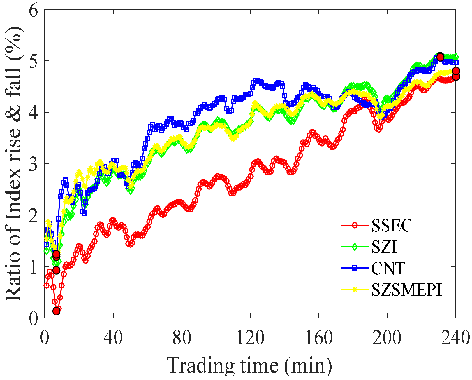
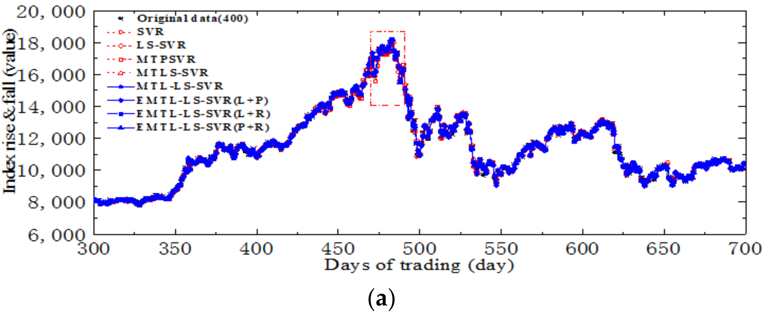
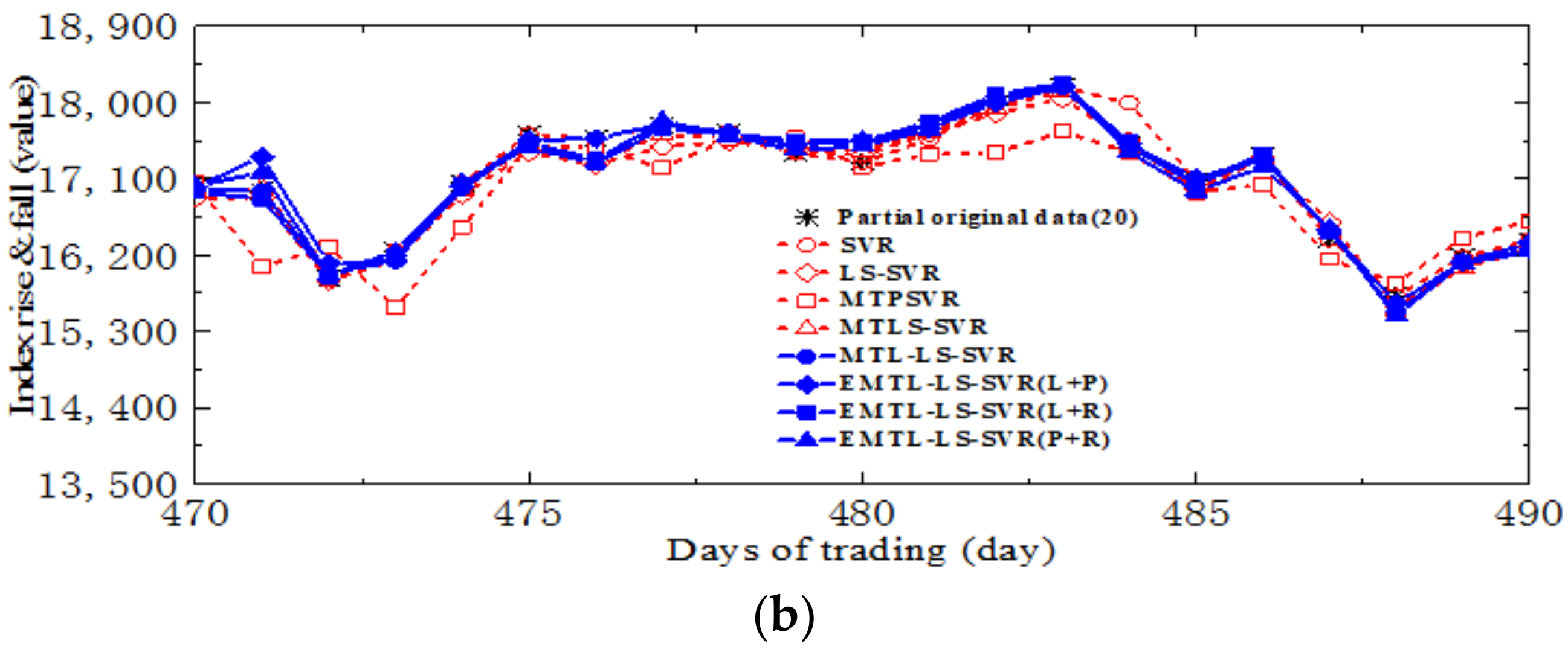
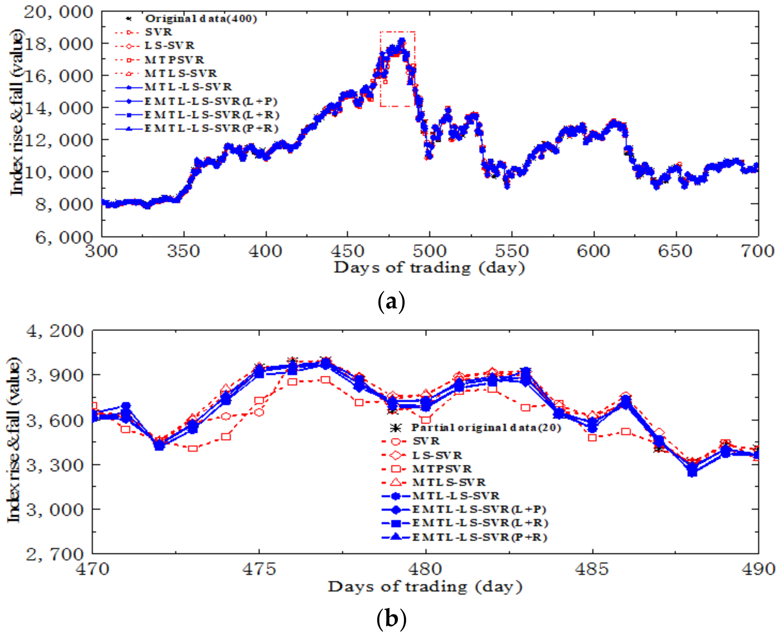
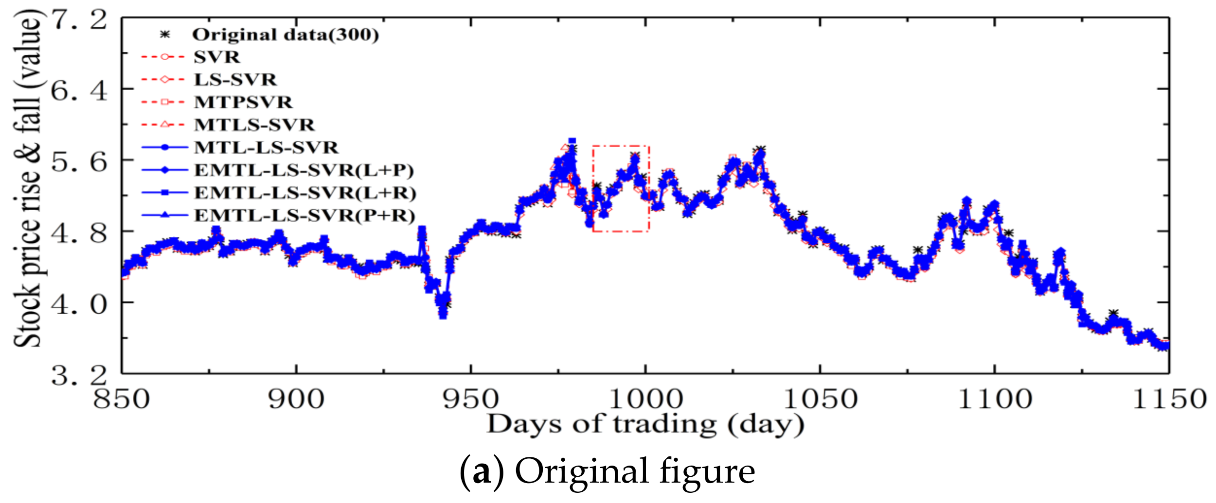
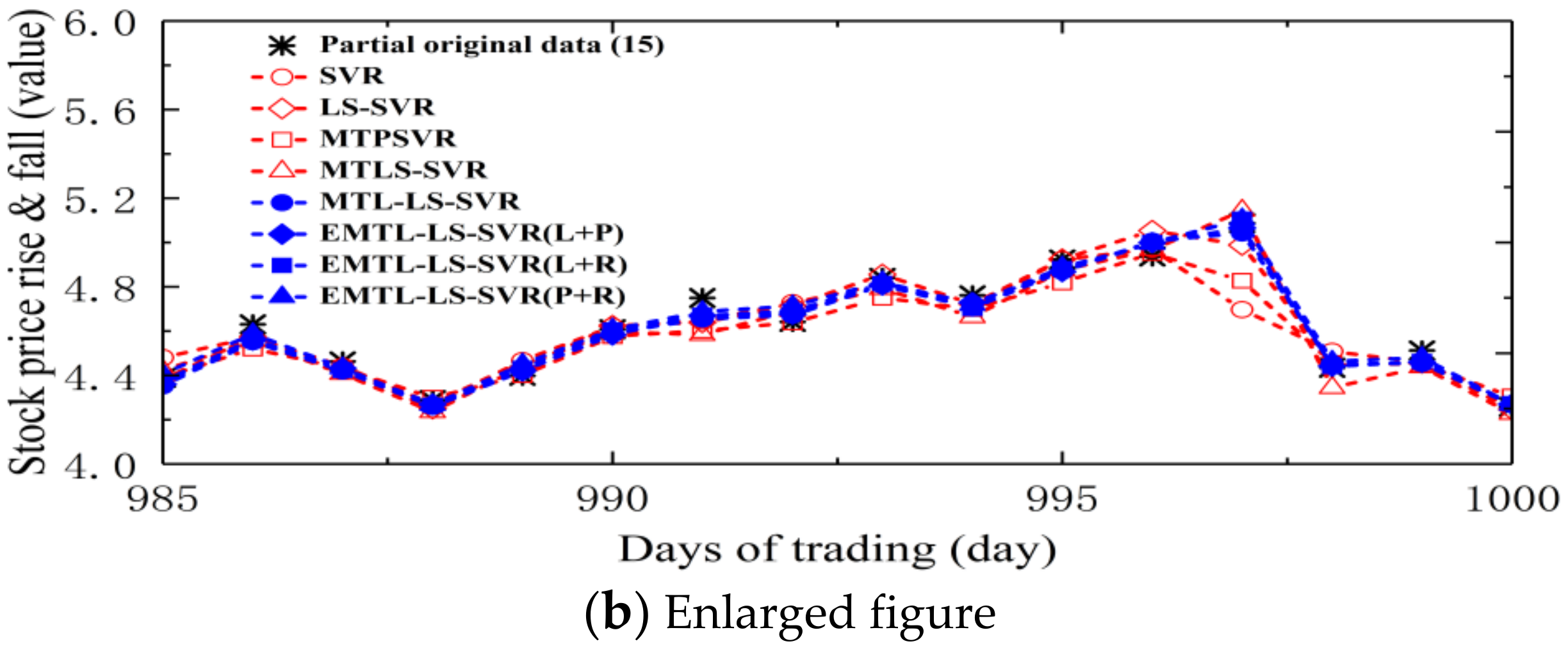
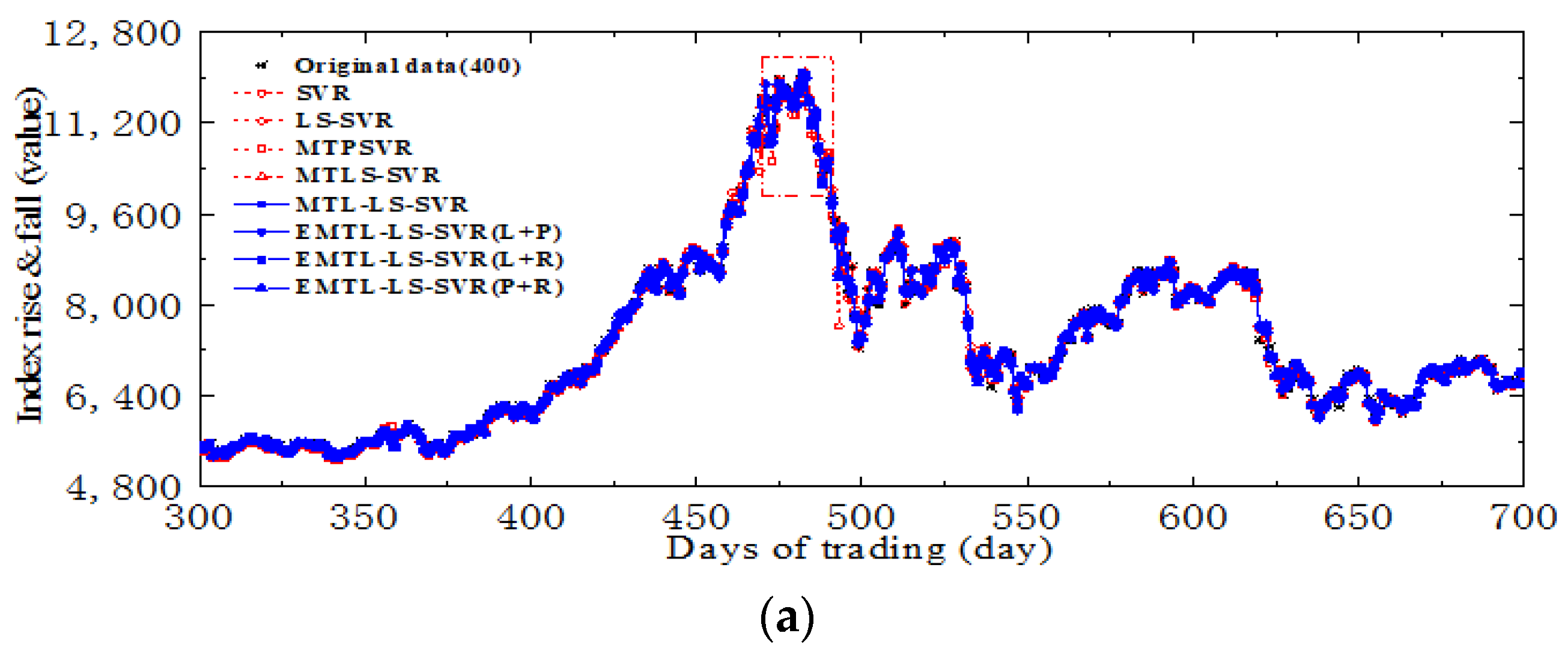
4.3. Forecast of Security of Stock Market Investment Environment

The running trend of the stock market index directly determines the security of the investment environment. Whether to prevent systemic structural risks or harvest dividends from stock market investments, accurate forecasts of the stock market index can provide much meaningful information. In this experiment, we verified the rationality of our models on stock index datasets, and applied them to forecast the opening index value of the stock market indices. The stock index datasets included historical data of the Shanghai Securities Composite Index (SSEC), a SZSE Composite Index (SZI), b Growth Enterprise Index (CNT), c and SSE SME Composite Index (SZSMEPI). d From the development history of the Chinese stock market, the crash effect of a rapid change from a bull market to a bear market was worse than for some international events, such as the Middle East Respiratory Syndrome Coronavirus (MERS-CoV) in 2012, and the 2019-nCoV out-broken in early 2020. Therefore, we selected an entire evolutionary period from a bull market to a bear market in Chinese stock market, with historical data including 1352 trading days, from 25 June 2013, to 4 January 2019. The data from each trading day were used as a sample point, with nine indicators: opening index, highest index value, lowest index value, closing index, index changing margin, index changing ratio, trading volume, trading amount, and previous day’s closing price. The four major stock market indices together compose the stock market of China, and they are affected by factors such as national policies, trade, and the international situation. We regard the above four stock indices as four subtasks, which are distinctive but interrelated, and which conform to the rules of multitask learning method.
To use multitask learning method to analyze the opening stock market index can make full use of the cross-correlation among different stock indices to obtain a more accurate prediction. Figure 3 shows the index time series change of the four indices on 1 June 2015. The horizontal axis represents the trading time (minutes) of stock trading in 240 min, and the vertical axis represents the change rate of each index on that day (taking the closing index of the last day as the baseline). Figure 3 shows that the movement of the four stock market indices is roughly the same, and they reach their highest and lowest points in the day at approximately the same times. These facts reflect their internal relationships.
a 
b 
c 
d 
To predict the opening index, we established a regression model based on the following assumptions. The opening index of a day is related to the other eight indicators of the previous day. The opening index of a day is the dependent variable, and the remaining indicators of the previous day are independent variables.
To verify the performance of the proposed regression models, eight algorithms were used to perform 20 independent runs on the stock index datasets. Table 1 lists the average results of 20 independent experiments. Figure 4, Figure 5, Figure 6 and Figure 7 show the predicted results for SSEC, SZI, CNT, and SZSMEPI, respectively. Considering the large number of training samples, only the forecast results of 400 continuous trading days during the peak period (11 September 2014, to 5 May 2016) are shown in Figure 4a, Figure 5a, Figure 6a and Figure 7a. To further compare the models, we enlarged the distinct parts labeled by the red dash-dot line that are 5% continuous trading days, and presented them in Figure 4b, Figure 5b, Figure 6b and Figure 7b. The red dashed lines with four different hollow symbols denote prediction results of the compared algorithms, and the blue solid lines with four different solid symbols represent the results of our proposed multitask learning models.
The experimental results of eight algorithms in predicting the stock indices are summarized in Table 1. For the M A E criterion, it is clear that SVR only has good results on the CNT dataset. The proposed multitask learning methods always produce the smallest S S E / S S T and S S R / S S T , and EMTL-LS-SVR in particular achieves significant performance. For the R M S E criterion, our MTL-LS-SVR models also achieve the best prediction results. In summary, SVR and MTLS-SVR have considerable learning effects, and the learning results of LS-SVR and MTPSVR are unsatisfactory compared to other regression methods. The results in Table 1 demonstrate that the learning effect of multitask learning models on different datasets can be further improved by selecting appropriate kernel functions and adjusting the relevant hyperparameters. Through experimental comparison, it is easy to find that when there is internal correlation among the learning tasks, multitask learning models can obtain much better prediction results than single-task learning methods. To select appropriate kernel functions for different information to establish the regression models also can greatly improve the learning effect.
Figure 4, Figure 5, Figure 6 and Figure 7 present the prediction results of the comparative algorithms on the four stock index datasets. In Figure 4a, Figure 5a, Figure 6a and Figure 7a, it can be seen that the eight methods produced apparent differences in the prediction results near the 480th day, which should be due to the mutual influences among stock indices. For clarity, the forecasting details of the stock indices for 20 continuous trading days around the 480th day are shown in Figure 4b, Figure 5b, Figure 6b and Figure 7b. It can be observed from Figure 4b, Figure 5b, Figure 6b and Figure 7b that MTPSVR and LS-SVR have larger deviations than MTL-LS-SVR. In addition, SVR and MTLS-SVR are comparable in learning and superior to MTPSVR, but they are still inferior to the proposed models. In Figure 4b, Figure 5b and Figure 6b, it can be observed that the four comparative regression models have obvious prediction deviations. In particular, MTPSVR produces relatively large prediction errors on many trading days.
The prediction results for stock indices shown in Figure 4, Figure 5, Figure 6 and Figure 7 and Table 1 further confirm the superior regression capability and robust performance of MTL-LS-SVR and EMTL-LS-SVR.

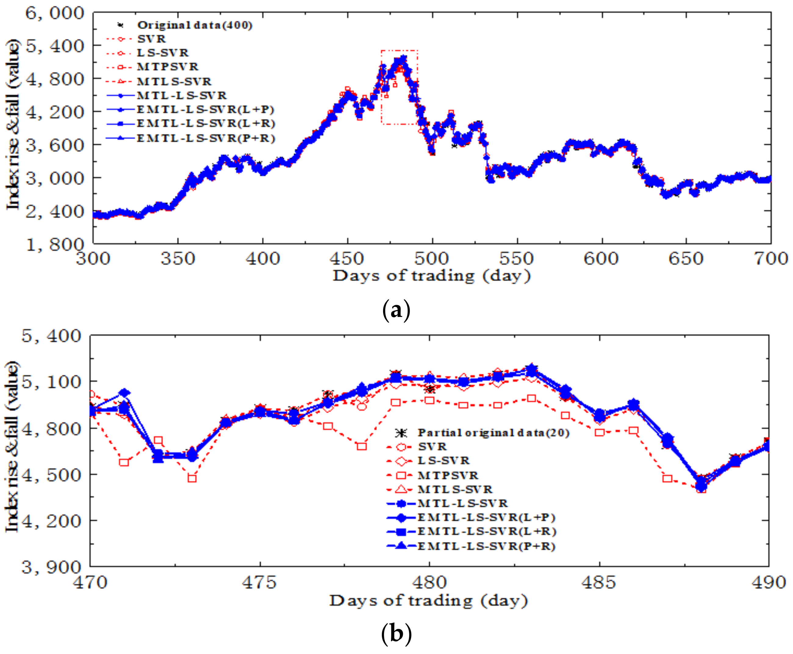
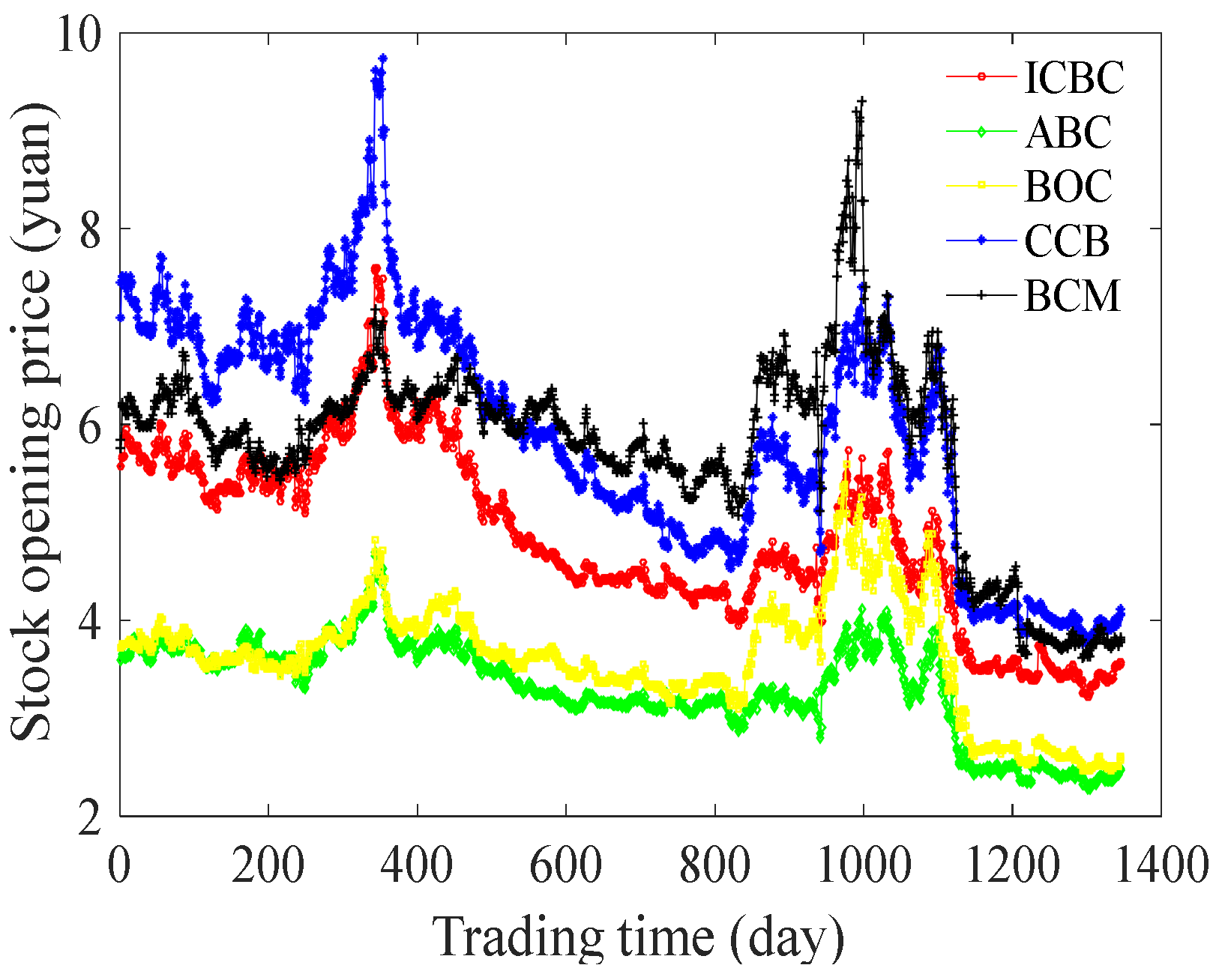
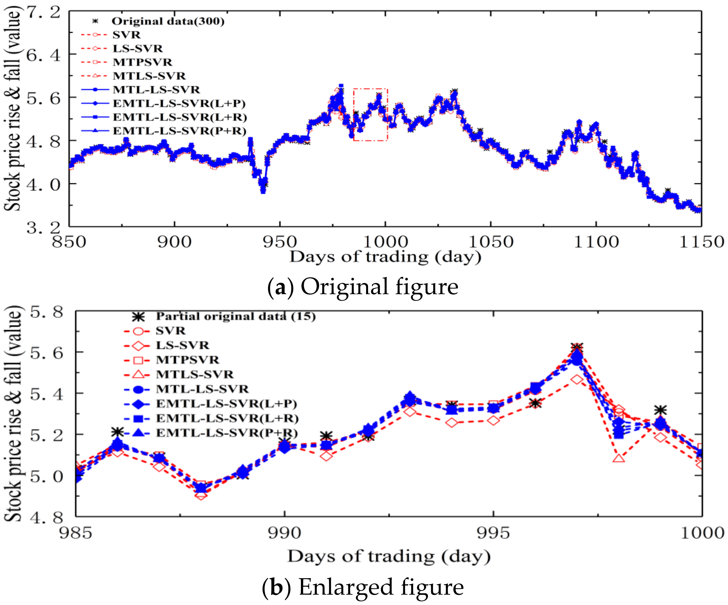
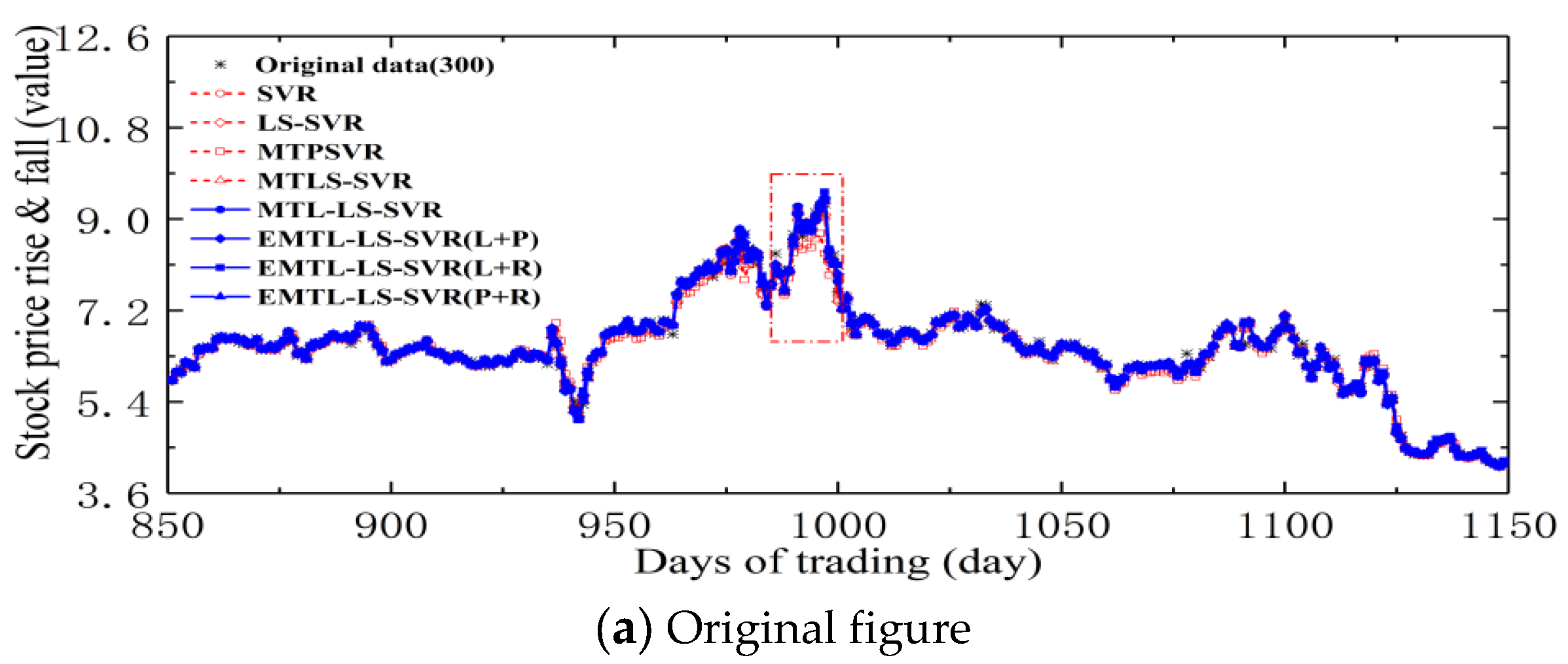
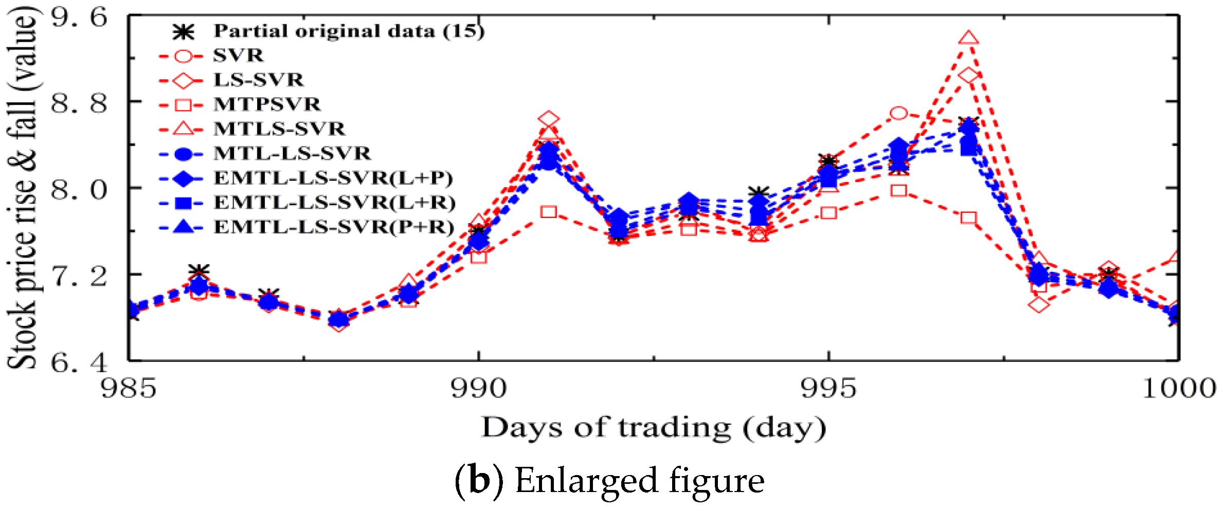
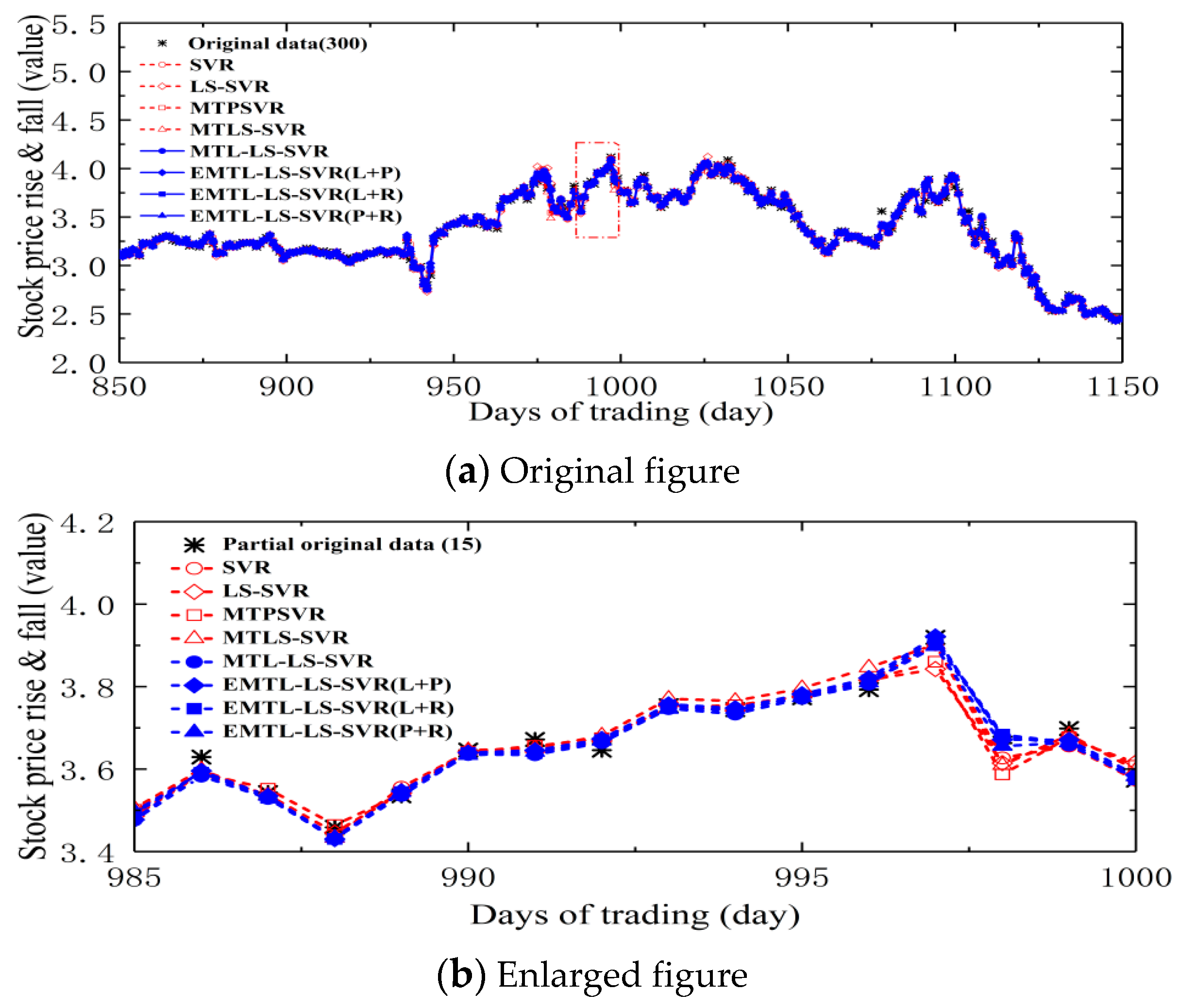
4.4. Forecasting Opening Prices of Five Major Banks

Accurate forecasts of the stock market index can help us to analyze future changes of the investment environment. Using the stock market index to guide real trading is the most critical issue for many investors. The five state-owned banks are important pillars of the Chinese banking industry, and their development is influenced by the country’s macroeconomic policies and the development of state-owned enterprises. Therefore, multitask learning models can be used to predict the banks’ stock price trends. In this experiment, we applied the proposed models to predict stock price trends of the five major state-owned banks. The bank datasets included 1346 days of trading data of the Industrial and Commercial Bank of China (ICBC), e Agricultural Bank of China (ABC), f Bank of China (BOC), g China Construction Bank CCB), h and Bank of Communications (BCM) i from 1 January 2014 to 10 July 2019. The data included eleven attribute indicators: opening price, highest price, lowest price, closing price, price changing margin, price changing ratio, trading volume, trading amount, trading amplitude, trading turnover rate, and previous day’s closing price. Therefore, five interrelated but different learning tasks were trained simultaneously, and used to confirm the accuracy of our proposed models. In the experiment, the opening price of the day is the dependent variable, and the remaining ten indicators of the previous day are independent variables. The stock (opening) prices on 1346 trading days are shown in Figure 8. It can be seen that the opening prices of the five major banks almost always fluctuated in the same direction, confirming a strong internal correlation among them.
e 
f 
g 
h 
i 
To evaluate the forecast results of the proposed models, eight algorithms were used to perform 20 independent runs on the bank datasets. Table 2 shows the average prediction results of 20 independent runs. Figure 9, Figure 10, Figure 11, Figure 12 and Figure 13 show the predictive effects of different regression methods for ICBC, ABC, BOC, CCB, and BCM, respectively. To more clearly distinguish the forecast effect of different models on the bank datasets, only the prediction results of the 300 continuous trading days from 28 June 2017, to 13 September 2018, are shown in Figure 9a, Figure 10a, Figure 11a, Figure 12a and Figure 13a. To further estimate the performance of the models, we selected some distinct forecast areas including 5% continuous trading days, which are marked by the red dash-dot line in Figure 9a, Figure 10a, Figure 11a, Figure 12a and Figure 13a. The comparison is shown in Figure 9b, Figure 10b, Figure 11b, Figure 12b and Figure 13b. In the experiment, the red dashed line with four different hollow symbols shows the prediction results of the compared single-task methods, and the blue solid line with four different solid patterns shows those of our proposed multitask learning models.
The experimental results of the eight algorithms for the bank datasets are generalized in Table 2. For the M A E criterion, it is clear that SVR has good results on the ABC and CCB datasets. The results show that our EMTL-LS-SVR models not only have the smallest but obtain the best results in terms of and criteria among the different regression models. It can be seen from Table 2 that EMTL-LS-SVR(L + P) achieves a better learning effect on the ABC and BOC datasets, whereas EMTL-LS-SVR(P + R) performs better on the other three banks’ data.
Figure 9, Figure 10, Figure 11, Figure 12 and Figure 13 show the forecasting results of the regression algorithms on the opening prices of the five major state-owned banks. To better distinguish the predictive effects of the different models on the bank datasets, Figure 9b, Figure 10b, Figure 11b, Figure 12b and Figure 13b present some significantly different areas, which are drawn based on the natural exponential function values corresponding to the source data. From Figure 9b, Figure 10b and Figure 11b, we can see that the fitting degrees of MTL-LS-SVR and EMTL-LS-SVR are preferable on the ICBC, ABC, and BOC stock datasets, whereas the prediction results obtained by LS-SVR, MTLS-SVR, and MTPSVR apparently differ from the real data. In Figure 12b and Figure 13b, the predictions of MTL-LS-SVR and EMTL-LS-SVR appear to have a slight deviation, perhaps because there is only a weak internal cross-correlation between CCB and BCM and the other state-owned banks. The fitting degree of SVR on CCB is better than that on the other state-owned banks, but it produces a high error on the 997th day in Figure 11b. MTPSVR also produces larger prediction deviations on the 998th day, as shown in Figure 10b. As shown in Figure 9b and Figure 12b, both LS-SVR and MTLS-SVR produce apparent prediction deviations over many trading days. In Figure 13b, it can be seen that MTPSVR produces relatively large prediction deviations over many trading days, and MTLS-SVR also produces an unsatisfactory prediction result on the 997th day.
The experimental results in Table 2 and Figure 9, Figure 10, Figure 11, Figure 12 and Figure 13 generally show that EMTL-LS-SVR and MTL-LS-SVR have better learning ability and more robust performance than the other models. The prediction results of different regression models for stock market indices and bank stock prices further verify their advantages. In summary, our proposed multitask learning models cannot only infer stock market crash signals but can accurately forecast stock price fluctuations. These results indicate that multitask learning models can capture the internal relationships among subtasks, and have more robust performance than single-task regression algorithms. In other words, multitask learning methods can use more information than single-task learning methods. Therefore, MTL-LS-SVR and EMTL-LS-SVR can achieve better learning effects.

5. Discussion

In the experiments section, the proposed multitask learning models are applied to perform forecasts of the Chinese stock market index trend and the stock prices of five stated-owned banks. In order to further discuss the performance differences between algorithms, the Friedman test with its corresponding Bonferroni-Dunn test [31] are employed for the experiments. For simplicity, we only analyze the prediction results of different algorithms on the two experimental datasets based on MAE and RMSE. Table 3 lists average ranks for all algorithms on two experimental datasets.
The Friedman test results are computed based on the two static parameters χ F 2 and F F . Based on the null hypothesis that all the algorithms are equivalent, the Friedman statistic can be computed by the following equations:
χ F 2 = 12 N K ( K + 1 ) i = 1 K R i 2 K ( K + 1 ) 2 4 ,
F F = ( N 1 ) χ F 2 N ( K 1 ) χ F 2 .
where N denotes the number of experiment datasets and K denotes the number of the comparative algorithms. R i = 1 N j = 1 N r j i is the average rank of the i - t h algorithm on the N experiment datasets used, and r j i represents the ranking of the prediction results of the i - t h algorithm on the j - t h experiment dataset among the K algorithms. F F is distributed according to the F -distribution with k 1 and k 1 N 1 degrees of freedom.
For this experiment, there are k = 8 and N = 9 . Based on the Equations (21) and (22), we can obtain χ F 2 47.937 and F F 25.459 for MAE criteria, and χ F 2 47.937 and F F 25.459 for RMSE criteria, where F F is distributed according to the F -distribution with k 1 N 1 = 56 degrees of freedom. The critical value of F 7 , 56 for significance level α = 0.05 is 2.178, which means the critical value is 2.178 based on a 95% confidence interval. For MAE and RMSE criteria, we find that the values of F F are much larger than the critical value, and thus the null hypothesis can be rejected and the eight algorithms have significant differences. Further, it can be seen from Table 3 that the proposed multitask learning models rank smaller than the other comparative algorithms and the EMTL-PSVM(L + R) obtain the smallest average rank for the MAE and RMSE criteria.
For further pairwise comparison, the Bonferroni-Dunn test is used [31]. The performance of two models are significantly different if their average ranks differ by more than the critical difference C D = q α K ( K + 1 ) 6 N . For this experiment, we find that q α = 2.829 for α = 0.1 and K = 8 , then we can obtain that C D = 2.829 . This means there is a 90% confidence level when the rank difference of two models is bigger than C D . Based on Table 3, we can compute the average rank deviations between the other methods and the EMTL-LS-SVR(L + R) for MAE as follows:
d ( S V R E M T L - L S - S V R ( L + R ) ) = 3.222 2.111 = 1.111 < 2.829 ,
d ( L S - S V R E M T L - L S - S V R ( L + R ) ) = 6.667 2.111 = 4.556 > 2.829 ,
d ( M T P S V R E M T L - L S - S V R ( L + R ) ) = 7.667 2.111 = 5.556 > 2.829 ,
d ( M T L S - S V R E M T L - L S - S V R ( L + R ) ) = 6.667 2.111 = 4.556 > 2.829 ,
d ( M T L - L S - S V R E M T L - L S - S V R ( L + R ) ) = 3.444 2.111 = 1.333 < 2.829 ,
d ( E M T L - L S - S V R ( L + P ) E M T L - L S - S V R ( L + R ) ) = 3.444 2.111 = 1.333 < 2.829 ,
d ( E M T L - L S - S V R ( P + R ) E M T L - L S - S V R ( L + R ) ) = 2.778 2.111 = 0.667 < 2.829 ,
where d ( a - b ) denotes the average rank deviations between the algorithm a and b . Similarly, the average rank differences between the other methods and the EMTL-LS-SVR(L + R) for RMSE can be expressed as follows:
d ( S V R E M T L - L S - S V R ( L + R ) ) = 5.222 2 = 3.222 > 2.829 ,
d ( L S - S V R E M T L - L S - S V R ( L + R ) ) = 7 2 = 5 > 2.829 ,
d ( M T P S V R E M T L - L S - S V R ( L + R ) ) = 7.333 2 = 5.333 > 2.829 ,
d ( M T L S - S V R E M T L - L S - S V R ( L + R ) ) = 6.444 2 = 4.444 > 2.829 ,
d ( M T L - L S - S V R E M T L - L S - S V R ( L + R ) ) = 2.444 2 = 0.444 < 2.829 ,
d ( E M T L - L S - S V R ( L + P ) E M T L - L S - S V R ( L + R ) ) = 3.556 2 = 1.556 < 2.829 ,
d ( E M T L - L S - S V R ( P + R ) E M T L - L S - S V R ( L + R ) ) = 2 2 = 0 < 2.829 .
In addition, Table 4 shows all of the comparison results between EMTL-LS-SVR(L + R) and the other comparative algorithms on the average rank deviations. The “Tag” represents the relation between d ( a - b ) and the C D value. “Tag” is 1 when d ( a - b ) is larger than C D ; otherwise, “Tag” is 0. From Table 4 can we know that, in terms of MAE criteria, the average rank difference between LS-SVR, MTPSVR, MTLS-SVR, and EMTL-LS-SVR(L + R) are larger than the critical value, which illustrates the performance of EMTL-LS-SVR(L + R) is significantly better than that of LS-SVR, MTPSVR, and MTLS-SVR. However, there are only slightly deviations between EMTL-LS-SVR(L + R) and SVR. For RMSE criteria, the performance of EMTL-PSVR(L + R) is superior to that of two single-task learning methods, MTPSVR and MTLS-SVR. Additionally, whether it is MAE or RMSE, there are slightly deviations between EMTL-LS-SVR(L + R) and other three forms, MTL-LS-SVR, EMTL-LS-SVR(L + P) and EMTL-LS-SVR(P + R).
In summary, the advantages of MTL-LS-SVR and its extension EMTL-LS-SVR are all evaluated whether from a experimental analysis view or from a statistical testing perspective. The superiority of MTL-LS-SVR and EMTL-LS-SVR models are benefited from they can effectively capture the correlation among multiple learning tasks to improve the prediction performance of the model. Meanwhile, selecting appropriate kernel functions for shared information and private information can more effectively deal with different information, which makes our proposed model have strong robust performance. For the fair, the traditional algorithms can achieve a better learning effect on the small-scale problems, while deep learning models have better advantages in dealing with large-scale data mining problems [32]. Therefore, how to effectively integrate multitask learning and deep learning to solve the real-world scenarios is also an attractive issue.

6. Conclusions

In this paper, we proposed an assumption that multiple related tasks share a common model and have their own independent models. Based on this assumption, we developed the MTL-LS-SVR model and an extension, EMTL-LS-SVR. MTL-LS-SVR makes good use of the advantages of least squares support vector regression and multitask learning. Meantime, the regularized parameter λ is introduced in MTL-LS-SVR and EMTL-LS-SVR to balance the shared information and private information among learning tasks. When learning tasks are related, superior performance can be achieved by adjusting λ and selecting appropriate kernel functions. Additionally, a Krylov-Cholesky algorithm is presented to optimize the solution procedures of the proposed models, which reduces the time to solve large-scale multitask learning problems. We tested the proposed models on the two stock datasets and compared the experimental results of different algorithms, which show that the EMTL-LS-SVR model can achieve a superior prediction effect and robust performance with the single-task learning method.
For the limitations of the MTL-LS-SVR algorithm, the correlations among learning tasks must be evaluated in advance when use it to make prediction and analysis on relevant real scenarios; otherwise, the learning effect may be weaker because of the potential negative transfer effect. Considering the advantages of neural networks, determining how to effectively apply the deep learning technique to solve multitask learning problems will be important future work for us.

Author Contributions

Conceptualization, H.-C.Z. and Q.W.; methodology, H.-C.Z. and F.-Y.L.; software, H.-C.Z.; validation, H.-C.Z., F.-Y.L. and Q.W.; formal analysis, Q.W.; investigation, H.-C.Z. and Q.W.; resources, Q.W.; data curation, H.-C.Z. and F.-Y.L.; writing—original draft preparation, H.-C.Z. and F.-Y.L.; writing—review and editing, H.-C.Z. and Q.W.; visualization, F.-Y.L.; supervision, Q.W. and H.L.; project administration, Q.W. and H.L.; funding acquisition, Q.W. and H.L. All authors have read and agreed to the published version of the manuscript.

Funding

This research was funded by the National Natural Science Foundation of China under Grants (51875457), the Key Research Project of Shaanxi Province (2022GY-028, 2022GY-050) and the Natural Science Foundation of Shaanxi Province (No. 2021JQ714).

Data Availability Statement

Not applicable.

Acknowledgments

Not applicable.

Conflicts of Interest

The authors declare no conflict of interest.

References

  1. Park, H.J.; Kim, Y.; Kim, H.Y. Stock market forecasting using a multi-task approach integrating long short-term memory and the random forest framework. Appl. Soft Comput. 2022, 114, 108106. [Google Scholar] [CrossRef]
  2. Kumbure, M.M.; Lohrmann, C.; Luukka, P.; Porras, J. Machine learning techniques and data for stock market forecasting: A literature review. Expert Syst. Appl. 2022, 197, 116659. [Google Scholar] [CrossRef]
  3. Kao, L.J.; Chiu, C.C.; Lu, C.J.; Yang, J.L. Integration of nonlinear independent component analysis and support vector regression for stock price forecasting. Neurocomputing. 2013, 99, 534–542. [Google Scholar] [CrossRef]
  4. Liang, M.X.; Wu, S.C.; Wang, X.L.; Chen, Q.C. A stock time series forecasting approach incorporating candlestick patterns and sequence similarity. Expert Syst. Appl. 2022, 205, 117295. [Google Scholar] [CrossRef]
  5. Yang, X.L.; Zhu, Y.; Cheng, T.Y. How the individual investors took on big data: The effect of panic from the internet stock message boards on stock price crash. Pac. Basin Financ. J. 2020, 59, 101245. [Google Scholar] [CrossRef]
  6. Ghosh, I.; Jana, R.K.; Sanyal, M.K. Analysis of temporal pattern, causal interaction and predictive modeling of financial markets using nonlinear dynamics, econometric models and machine learning algorithms. Appl. Soft Comput. 2019, 82, 105553. [Google Scholar] [CrossRef]
  7. Yu, X.J.; Wang, Z.L.; Xiao, W.L. Is the nonlinear hedge of options more effective?—Evidence from the SSE 50 ETF options in China. North Am. J. Econ. Financ. 2019, 54, 100916. [Google Scholar] [CrossRef]
  8. Chen, Y.S.; Cheng, C.H.; Chiu, C.L.; Huang, S.T. A study of ANFIS-based multi-factor time series models for forecasting stock index. Appl. Intell. 2016, 45, 277–292. [Google Scholar] [CrossRef]
  9. Huang, L.X.; Li, W.; Wang, H.; Wu, L.S. Stock dividend and analyst optimistic bias in earnings forecast. Int. Rev. Econ. Financ. 2022, 78, 643–659. [Google Scholar] [CrossRef]
  10. Chalvatzis, C.; Hristu-Varsakelis, D. High-performance stock index trading via neural networks and trees. Appl. Soft Comput. 2020, 96, 106567. [Google Scholar] [CrossRef]
  11. Zhang, J.; Teng, Y.F.; Chen, W. Support vector regression with modified firefly algorithm for stock price forecasting. Appl. Intell. 2019, 49, 1658–1674. [Google Scholar] [CrossRef]
  12. Cao, J.S.; Wang, J.H. Exploration of stock index change prediction model based on the combination of principal component analysis and artificial neural network. Soft Comput. 2020, 24, 7851–7860. [Google Scholar] [CrossRef]
  13. Qiu, Y.; Yang, H.W.; Chen, W. A novel hybrid model based on recurrent neural networks for stock market timing. Soft Comput. 2020, 24, 15273–15290. [Google Scholar] [CrossRef]
  14. Song, Y.; Lee, J.W.; Lee, J. A study on novel filtering and relationship between input-features and target-vectors in a deep learning model for stock price prediction. Appl. Intell. 2019, 49, 897–911. [Google Scholar] [CrossRef]
  15. Ojo, S.O.; Owolawi, P.A.; Mphahlele, M.; Adisa, J.A. Stock Market Behaviour Prediction using Stacked LSTM Networks. Proceeding of the 2019 International Multidisciplinary Information Technology and Engineering Conference (IMITEC), Vanderbijlpark, South Africa, 21–22 November 2019; pp. 1–5. [Google Scholar] [CrossRef]
  16. Li, X.D.; Xie, H.R.; Wang, R.; Cai, Y.; Cao, J.J.; Wang, F.; Min, H.Q.; Deng, X.T. Empirical analysis: Stock market prediction via extreme learning machine. Neural Comput. Appl. 2016, 27, 67–68. [Google Scholar] [CrossRef]
  17. Dash, R.; Dash, P.K. Efficient stock price prediction using a self evolving recurrent neuro-fuzzy inference system optimized through a modified differential harmony search technique. Expert Syst. Appl. 2016, 52, 75–90. [Google Scholar] [CrossRef]
  18. Kalra, S.; Prasad, J.S. Efficacy of news sentiment for stock market prediction. Proceeding of the 2019 International Conference on Machine Learning, Big Data, Cloud and Parallel Computing (COMITCon), Faridabad, India, 14–16 February 2019; pp. 491–496. [Google Scholar] [CrossRef]
  19. Lim, M.W.; Yeo, C.K. Harvesting social media sentiments for stock index prediction. Proceeding of the 2020 IEEE 17th Annual Consumer Communications & Networking Conference (CCNC), Las Vegas, NV, USA, 10–13 January 2020; pp. 1–4. [Google Scholar] [CrossRef]
  20. Mohanty, D.K.; Parida, A.K.; Khuntia, S.S. Financial market prediction under deep learning framework using auto encoder and kernel extreme learning machine. Appl. Soft Comput. 2021, 99, 106898. [Google Scholar] [CrossRef]
  21. Mahmoud, R.A.; Hajj, H.; Karameh, F.N. A systematic approach to multi-task learning from time-series data. Appl. Soft Comput. 2020, 96, 106586. [Google Scholar] [CrossRef]
  22. Gao, P.X. Facial age estimation using clustered multi-task support vector regression machine. Proceeding of the 21st International Conference on Pattern Recognition (ICPR2012), Tsukuba, Japan, 11–15 November 2012; pp. 541–544. Available online: https://ieeexplore.ieee.org/document/6460191 (accessed on 29 April 2022).
  23. Li, Y.; Tian, X.M.; Song, M.L.; Tao, D.C. Multi-task proximal support vector machine. Pattern Recognit. 2015, 48, 3249–3257. [Google Scholar] [CrossRef]
  24. Xu, S.; An, X.; Qiao, X.D.; Zhu, L.J. Multi-task least-squares support vector machines. Multimed. Tools Appl. 2014, 71, 699–715. [Google Scholar] [CrossRef]
  25. Anand, P.; Rastogi, R.; Chandra, S. A class of new support vector regression models. Appl. Soft Comput. 2020, 94, 106446. [Google Scholar] [CrossRef]
  26. Hong, X.; Mitchell, R.; Fatta, G.D. Simplex basis function based sparse least squares support vector regression. Neurocomputing. 2019, 330, 394–402. [Google Scholar] [CrossRef] [Green Version]
  27. Choudhary, R.; Ahuja, K. Stability analysis of Bilinear Iterative Rational Krylov algorithm. Linear Algebra Its Appl. 2018, 538, 56–88. [Google Scholar] [CrossRef] [Green Version]
  28. Samar, M.; Farooq, A.; Li, H.Y.; Mu, C.L. Sensitivity analysis for the generalized Cholesky factorization. Appl. Math. Comput. 2019, 362, 124556. [Google Scholar] [CrossRef]
  29. Xue, Y.T.; Zhang, L.; Wang, B.J.; Zhang, Z.; Li, F.Z. Nonlinear feature selection using Gaussian kernel SVM-RFE for fault diagnosis. Appl. Intell. 2018, 48, 3306–3331. [Google Scholar] [CrossRef]
  30. Xu, Y.T.; Li, X.Y.; Pan, X.L.; Yang, Z.J. Asymmetric ν-twin support vector regression. Neural Comput. Appl. 2018, 30, 3799–3814. [Google Scholar] [CrossRef]
  31. Wang, E.; Wang, Z.Y.; Wu, Q. One novel class of Bézier smooth semi-supervised support vector machines for classification. Neural Comput. Appl. 2021, 33, 9975–9991. [Google Scholar] [CrossRef]
  32. Qin, W.T.; Tang, J.; Lu, C.; Lao, S.Y. A typhoon trajectory prediction model based on multimodal and multitask learning. Appl. Soft Comput. 2022, 122, 108804. [Google Scholar] [CrossRef]
Figure 1. Block diagram of MTL-LS-SVR and EMTL-LS-SVR.
Axioms 11 00292 g001
Figure 2. Flowchart of MTL-LS-SVR and EMTL-LS-SVR models.
Axioms 11 00292 g002
Figure 3. Movement of stock market indices on 1 June 2015.
Axioms 11 00292 g003
Figure 4. Predictions of different regression models on opening index for SSEC (a) Original figure, (b) Enlarged figure.
Axioms 11 00292 g004
Figure 5. Predictions of different regression models on opening index for SZI (a) Original figure, (b) Enlarged figure.
Axioms 11 00292 g005aAxioms 11 00292 g005b
Figure 6. Predictions of different regression models on opening index for CNT (a) Original figure, (b) Enlarged figure.
Axioms 11 00292 g006
Figure 7. Predictions of different regression models on opening index for SZSMEPI (a) Original figure, (b) Enlarged figure.
Axioms 11 00292 g007aAxioms 11 00292 g007b
Figure 8. Change of stock opening prices of five stated banks.
Axioms 11 00292 g008
Figure 9. Predictions of different regression models on stock opening price for ICBC (a) Original figure, (b) Enlarged figure.
Axioms 11 00292 g009
Figure 10. Predictions of different regression models on stock opening price for ABC (a) Original figure, (b) Enlarged figure.
Axioms 11 00292 g010
Figure 11. Predictions of different regression models on stock opening price for BOC (a) Original figure, (b) Enlarged figure.
Axioms 11 00292 g011aAxioms 11 00292 g011b
Figure 12. Predictions of different regression models on stock opening price for CCB (a) Original figure, (b) Enlarged figure.
Axioms 11 00292 g012
Figure 13. Predictions of different regression models on stock opening price for BCM (a) Original figure, (b) Enlarged figure.
Axioms 11 00292 g013aAxioms 11 00292 g013b
Table 1. Performance comparisons of eight algorithms on four major stock market indices.
Stock IndexAlgorithmMAERMSESSE/SSTSSR/SST(C,σ,λ,d)
SSECSVR8.7363 ± 0.610015.0791 ± 2.97350.0007 ± 0.00030.9992 ± 0.0041(55,3.85,~,~)
LS-SVR9.8034 ± 0.988417.1879 ± 3.05980.0008 ± 0.00030.9961 ± 0.0064(100,1.85,~,~)
MTPSVR10.299 ± 1.708118.9993 ± 2.96560.0010 ± 0.00030.9990 ± 0.0090(80,3.45,0.21,~)
MTLS-SVR9.083 ± 1.856516.5463 ± 3.68390.0008 ± 0.00041.0038 ± 0.0070(70,2.65,1.26,~)
MTL-LS-SVR7.0850 ± 1.208112.1375 ± 2.96560.0005 ± 0.00031.0134 ± 0.0090(100,2.25,0.11,~)
EMTL-LS-SVR(L + P)8.7002 ± 1.856513.1821 ± 3.68390.0006 ± 0.00041.0180 ± 0.0070(85,~,1.81,2)
EMTL-LS-SVR(L + R)8.2580 ± 0.987014.5139 ± 2.22110.0006 ± 0.00021.0152 ± 0.0067(95,2.65,1.31,~)
EMTL-LS-SVR(P + R)7.9055 ± 1.419512.1985 ± 3.33300.0004 ± 0.00031.0147 ± 0.0065(100,1.85,0.86,2)
SZISVR34.307 ± 3.289460.0911 ± 10.2630.0010 ± 0.00031.0027 ± 0.0070(55,3.85,~,~)
LS-SVR39.772 ± 4.139865.2855 ± 10.6490.0012 ± 0.00040.9983 ± 0.0066(85,0.65,~,~)
MTPSVR41.355 ± 7.793270.3547 ± 14.5350.0013 ± 0.00051.0042 ± 0.0101(80,3.45,0.21,~)
MTLS-SVR35.049 ± 4.887958.0722 ± 7.95870.0010 ± 0.00021.0010 ± 0.0102(70,2.65,1.26,~)
MTL-LS-SVR30.323 ± 7.793247.9612 ± 14.5350.0008 ± 0.00051.0238 ± 0.0101(100,2.25,0.11,~)
EMTL-LS-SVR(L + P)31.789 ± 4.887948.0880 ± 7.95870.0006 ± 0.00021.0305 ± 0.0102(85,~,1.81,2)
EMTL-LS-SVR(L + R)31.278 ± 3.688250.9115 ± 6.55260.0007 ± 0.00021.0134 ± 0.0060(95,2.65,1.31,~)
EMTL-LS-SVR(P + R)34.269 ± 6.711157.4735 ± 12.6800.0008 ± 0.00051.0268 ± 0.0096(100,1.85,0.86,2)
CNTSVR6.6680 ± 0.604313.3354 ± 2.09720.0007 ± 0.00021.0035 ± 0.0081(65,3.05,~,~)
LS-SVR9.6897 ± 0.872817.6334 ± 2.20480.0012 ± 0.00030.9974 ± 0.0139(100,1.05,~,~)
MTPSVR10.483 ± 1.587417.1729 ± 2.14070.0012 ± 0.00031.0006 ± 0.0088(80,3.45,0.21,~)
MTLS-SVR9.3258 ± 1.272115.4848 ± 1.80140.0010 ± 0.00030.9985 ± 0.0090(70,2.65,1.26,~)
MTL-LS-SVR8.8047 ± 1.587412.9715 ± 2.14070.0008 ± 0.00031.0121 ± 0.0088(100,2.25,0.11,~)
EMTL-LS-SVR(L + P)7.5338 ± 1.272112.0025 ± 1.80140.0005 ± 0.00031.0152 ± 0.0090(85,~,1.81,2)
EMTL-LS-SVR(L + R)7.6653 ± 0.779113.2993 ± 1.36320.0007 ± 0.00021.0170 ± 0.0095(95,2.65,1.31,~)
EMTL-LS-SVR(P + R)8.1940 ± 1.836612.9907 ± 2.52600.0008 ± 0.00031.0162 ± 0.0110(100,1.85,0.86,2)
SZSMEPISVR24.642 ± 1.622042.3225 ± 5.76390.0010 ± 0.00021.0015 ± 0.0058(80,1.45,~,~)
LS-SVR26.818 ± 1.798642.5460 ± 5.20530.0011 ± 0.00020.9979 ± 0.0068(100,0.95,~,~)
MTPSVR28.393 ± 4.860947.7573 ± 10.4860.0013 ± 0.00060.9975 ± 0.0100(80,3.45,0.21,~)
MTLS-SVR25.043 ± 3.202942.4982 ± 7.46060.0011 ± 0.00031.0019 ± 0.0052(70,2.65,1.26,~)
MTL-LS-SVR19.548 ± 2.360930.7638 ± 10.4860.0006 ± 0.00061.0170 ± 0.0100(100,2.25,0.11,~)
EMTL-LS-SVR(L + P)20.723 ± 3.202935.2842 ± 7.46060.0006 ± 0.00031.0105 ± 0.0052(85,~,1.81,2)
EMTL-LS-SVR(L + R)22.228 ± 1.649234.3454 ± 3.95920.0007 ± 0.00011.0146 ± 0.0062(95,2.65,1.31,~)
EMTL-LS-SVR(P + R)20.014 ± 4.235732.6555 ± 8.31700.0007 ± 0.00041.0157 ± 0.0071(100,1.85,0.86,2)
Table 2. Performance comparisons of eight algorithms on stock data of China’s five state banks.
Bank Stock PriceAlgorithmMAERMSESSE/SSTSSR/SST(C,σ,λ,d)
ICBCSVR0.0144 ± 0.00120.0245 ± 0.00490.0008 ± 0.00030.9980 ± 0.0050(80,2.25,~,~)
LS-SVR0.0196 ± 0.00150.0276 ± 0.00700.0010 ± 0.00050.9968 ± 0.0070(70,0.65,~,~)
MTPSVR0.0252 ± 0.00250.0263 ± 0.00600.0011 ± 0.00050.9939 ± 0.0124(75,2.25,0.06,~)
MTLS-SVR0.0263 ± 0.00320.0278 ± 0.00750.0010 ± 0.00080.9978 ± 0.0157(75,3.05,1.81,~)
MTL-LS-SVR0.0145 ± 0.00250.0220 ± 0.00600.0006 ± 0.00051.0109 ± 0.0124(90,3.45,0.91,~)
EMTL-LS-SVR(L + P)0.0164 ± 0.00320.0230 ± 0.00750.0007 ± 0.00081.0487 ± 0.0157(100,~,1.61,2)
EMTL-LS-SVR(L + R)0.0156 ± 0.00370.0232 ± 0.00920.0006 ± 0.00081.0088 ± 0.0115(100,1.45,1.41,~)
EMTL-LS-SVR(P + R)0.0143 ± 0.00120.0203 ± 0.00630.0005 ± 0.00051.0146 ± 0.0086(85,1.45,0.46,2)
ABCSVR0.0098 ± 0.00090.0171 ± 0.00330.0013 ± 0.00050.9989 ± 0.0032(50,3.45,~,~)
LS-SVR0.0110 ± 0.00080.0184 ± 0.00270.0015 ± 0.00040.9964 ± 0.0046(90,1.45,~,~)
MTPSVR0.0137 ± 0.00210.0211 ± 0.00400.0019 ± 0.00071.0038 ± 0.0216(75,2.25,0.06,~)
MTLS-SVR0.0124 ± 0.00190.0216 ± 0.00620.0021 ± 0.00140.9975 ± 0.0101(75,3.05,1.81,~)
MTL-LS-SVR0.0100 ± 0.00210.0150 ± 0.00400.0010 ± 0.00071.0505 ± 0.0216(90,3.45,0.91,~)
EMTL-LS-SVR(L + P)0.0101 ± 0.00190.0147 ± 0.00280.0008 ± 0.00051.0141 ± 0.0101(100,~,1.61,2)
EMTL-LS-SVR(L + R)0.0105 ± 0.00150.0167 ± 0.00340.0011 ± 0.00061.0130 ± 0.0117(100,1.45,1.41,~)
EMTL-LS-SVR(P + R)0.0096 ± 0.00090.0149 ± 0.00330.0009 ± 0.00061.0253 ± 0.0111(85,1.45,0.46,2)
BOCSVR0.0120 ± 0.00130.0250 ± 0.00550.0019 ± 0.00080.9998 ± 0.0084(70,3.85,~,~)
LS-SVR0.0134 ± 0.00150.0262 ± 0.00560.0021 ± 0.00090.9973 ± 0.0069(95,2.25,~,~)
MTPSVR0.0164 ± 0.00300.0278 ± 0.00610.0024 ± 0.00100.9991 ± 0.0210(75,2.25,0.06,~)
MTLS-SVR0.0153 ± 0.00190.0272 ± 0.00600.0025 ± 0.00110.9971 ± 0.0122(75,3.05,1.81,~)
MTL-LS-SVR0.0128 ± 0.00300.0189 ± 0.00610.0011 ± 0.00101.0424 ± 0.0210(90,3.45,0.91,~)
EMTL-LS-SVR(L + P)0.0113 ± 0.00190.0177 ± 0.00600.0009 ± 0.00111.0209 ± 0.0122(100,~,1.61,2)
EMTL-LS-SVR(L + R)0.0118 ± 0.00210.0190 ± 0.00700.0010 ± 0.00121.0159 ± 0.0176(100,1.45,1.41,~)
EMTL-LS-SVR(P + R)0.0118 ± 0.00150.0182 ± 0.00620.0010 ± 0.00111.0433 ± 0.0162(85,1.45,0.46,2)
CCBSVR0.0203 ± 0.00180.0376 ± 0.00550.0010 ± 0.00030.9979 ± 0.0042(50,3.85,~,~)
LS-SVR0.0264 ± 0.00140.0510 ± 0.00480.0016 ± 0.00030.9946 ± 0.0048(85,0.65,~,~)
MTPSVR0.0238 ± 0.00560.0432 ± 0.00700.0013 ± 0.00040.9956 ± 0.0246(75,2.25,0.06,~)
MTLS-SVR0.0245 ± 0.00730.0509 ± 0.01420.0015 ± 0.00110.9961 ± 0.0133(75,3.05,1.81,~)
MTL-LS-SVR0.0208 ± 0.00560.0327 ± 0.00700.0007 ± 0.00041.0558 ± 0.0246(90,3.45,0.91,~)
EMTL-LS-SVR(L + P)0.0224 ± 0.00730.0330 ± 0.01420.0007 ± 0.00111.0134 ± 0.0133(100,~,1.61,2)
EMTL-LS-SVR(L + R)0.0225 ± 0.00310.0374 ± 0.00550.0009 ± 0.00031.0098 ± 0.0121(100,1.45,1.41,~)
EMTL-LS-SVR(P + R)0.0208 ± 0.00240.0316 ± 0.00460.0006 ± 0.00051.0118 ± 0.0097(85,1.45,0.46,2)
BCMSVR0.0204 ± 0.00210.0430 ± 0.00690.0021 ± 0.00060.9970 ± 0.0162(80,2.85,~,~)
LS-SVR0.0245 ± 0.00250.0483 ± 0.00670.0027 ± 0.00070.9924 ± 0.0154(75,1.85,~,~)
MTPSVR0.0278 ± 0.00280.0565 ± 0.00820.0031 ± 0.00080.9916 ± 0.0205(75,2.25,0.06,~)
MTLS-SVR0.0259 ± 0.00390.0418 ± 0.01210.0025 ± 0.00130.9996 ± 0.0163(75,3.05,1.81,~)
MTL-LS-SVR0.0203 ± 0.00280.0333 ± 0.00820.0011 ± 0.00081.0370 ± 0.0205(90,3.45,0.91,~)
EMTL-LS-SVR(L + P)0.0220 ± 0.00390.0352 ± 0.01210.0014 ± 0.00131.0404 ± 0.0163(100,~,1.61,2)
EMTL-LS-SVR(L + R)0.0195 ± 0.00530.0308 ± 0.01030.0013 ± 0.00101.0270 ± 0.0187(100,1.45,1.41,~)
EMTL-LS-SVR(P + R)0.0191 ± 0.00220.0278 ± 0.00890.0012 ± 0.00081.0242 ± 0.0138(85,1.45,0.46,2)
Table 3. Average ranks of all algorithms in the Friedman test on the two experimental datasets.
AlgorithmMetricSSECSZICNTSZSMEPIICBCABCBOCCCBBCMp-Value
SVRMAE5515224143.222
RMSE5655555565.222
LS-SVRMAE7777666866.667
RMSE7787766877
MTPSVRMAE8888788687.667
RMSE8878678687.333
MTLS-SVRMAE6666877776.667
RMSE6566887756.444
MTL-LS-SVRMAE4323541453.444
RMSE3214311342.444
EMTL-LS-SVR(L + P)MAE3234453523.444
RMSE4343444423.556
EMTL-LS-SVR(L + R)MAE2442112212.111
RMSE2432122112
EMTL-LS-SVR(P + R)MAE1151335332.778
RMSE1121233232
Table 4. Comparison results between EMTL-LS-SVR(L + R) and other algorithms on average rank deviations.
Title 1MAETagRMSETag
SVR1.11103.2221 *
LS-SVR4.5561 **51 ***
MTPSVR5.5561 ***5.3331 ***
MTLS-SVR4.5561 **4.4441 **
MTL-LS-SVR1.33300.4440
EMTL-LS-SVR(L + P)1.33301.5560
EMTL-LS-SVR(P + R)0.667000
Remark: In Table 4, set d to represent the absolute value of the difference between average rank deviation and the C D value. * denotes d is between [0, 1], ** denotes d is between [1, 2], *** denotes d is between [2, 3], **** denotes d is between [3, 4].
Publisher’s Note: MDPI stays neutral with regard to jurisdictional claims in published maps and institutional affiliations.

